| Issue |
A&A
Volume 702, October 2025
|
|
|---|---|---|
| Article Number | A116 | |
| Number of page(s) | 16 | |
| Section | Stellar structure and evolution | |
| DOI | https://doi.org/10.1051/0004-6361/202452118 | |
| Published online | 14 October 2025 | |
Matching seismic masses for RR Lyrae-type and oscillating red horizontal branch stars in M4
1
Konkoly Observatory, HUN-REN Research Centre for Astronomy and Earth Sciences, MTA Centre of Excellence, Konkoly-Thege Miklós út 15-17, H-1121 Budapest, Hungary
2
ELTE Eötvös Loránd University, Institute of Physics and Astronomy, 1117 Pázmány Péter sétány 1/A, Budapest, Hungary
3
Institute of Physics, École Polytechnique Fédérale de Lausanne (EPFL), Observatoire de Sauverny, 1290 Versoix, Switzerland
4
Nicolaus Copernicus Astronomical Centre, Polish Academy of Sciences, Bartycka 18, PL-00-716 Warszawa, Poland
5
Department of Astronomy, The Ohio State University, 140 W. 18th Ave., Columbus, OH 43210
USA
6
Center for Cosmology and Astroparticle Physics (CCAPP), The Ohio State University, 191 W. Woodruff Avenue, Columbus, OH 43210
USA
7
University of Wyoming, 1000 E University Ave, Laramie, WY USA
⋆ Corresponding author: This email address is being protected from spambots. You need JavaScript enabled to view it.
; This email address is being protected from spambots. You need JavaScript enabled to view it.
Received:
5
September
2024
Accepted:
28
July
2025
Abstract
Globular clusters offer a powerful way to test the properties of stellar populations and the late stages of low-mass stellar evolution. For this paper we studied oscillating giant stars and overtone RR Lyrae-type pulsators in the nearest globular cluster, M4, with the help of high-precision, continuous light curves collected by the Kepler space telescope in the K2 mission. We determined the frequency composition of five RRc stars and modeled their physical parameters from linear pulsation models. We were able, for the first time, to compare seismic masses of RR Lyrae stars directly to the masses of the very similar red horizontal branch stars in the same stellar population, independently determined from asteroseismic scaling relations. We find average seismic masses of 0.648 ± 0.028 M⊙ for RR Lyrae stars and 0.657 ± 0.034 M⊙ for red horizontal branch stars. While the accuracy of our RR Lyrae masses still relies on the accuracy of evolutionary mass differences of neighboring horizontal branch subgroups, this result strongly indicates that RRc stars may indeed exhibit high-degree ℓ = 8 and 9 nonradial modes, and modeling these modes can provide realistic mass estimates. We compare the seismic masses of our red horizontal branch and RR Lyrae stars to evolutionary models and to theoretical mass relations, and highlight the limitations of these relations.
Key words: asteroseismology / stars: horizontal-branch / stars: variables: RR Lyrae / globular clusters: individual: M4
© The Authors 2025
 Open Access article, published by EDP Sciences, under the terms of the Creative Commons Attribution License (https://creativecommons.org/licenses/by/4.0), which permits unrestricted use, distribution, and reproduction in any medium, provided the original work is properly cited.
This article is published in open access under the Subscribe to Open model. This email address is being protected from spambots. You need JavaScript enabled to view it. to support open access publication.
1. Introduction
Masses of RR Lyrae stars are notoriously difficult to determine. This is a problem because the masses of horizontal branch (HB) stars and in particular the masses of RR Lyrae stars that are located at the intersection of the HB and the instability strip of classical pulsating stars, are crucial pieces of information for stellar evolution theories and models (Catelan 2009). Masses would provide information not only on the mass distribution along the HB, but also on the amount of mass loss during the red giant phase of stellar evolution and on the accuracy of mass estimates based on pulsational envelope models as well. Thus, many avenues of research have already been explored to determine the masses of RR Lyrae stars.
Binarity, for example, would be a straightforward way to infer dynamical masses. However, not only do we not know any eclipsing binaries with an RR Lyrae member, it is very difficult to find systems that contain an RR Lyrae star at all (Wade et al. 1999; Kennedy et al. 2014; Hajdu et al. 2015; Liška et al. 2016a). Since bona fide RR Lyrae stars are considered to be very old. Their companions have either evolved into white dwarfs or other stellar remnants already, or must be smaller stars, most likely still evolving along the lower main sequence as K–M dwarfs. This means that the contribution of RR Lyr companions to the total light output of the system is expected to be minimal, precluding the detection via spectral energy distribution as double-lined spectroscopic binaries.
The dearth of eclipsing RR Lyrae stars can also be explained by the evolutionary pathways of these pulsators. These stars moved past the red giant phase without any significant interactions with a companion that could have directed the primary away from evolving onto the HB and toward binary evolution scenarios. Companions thus must be distant to avoid any mass transfer, and a distant companion orbiting a now shrunken HB star would make the probability of observing the expected shallow eclipses from the system very low. The only eclipsing binary candidate system turned out to be an “impostor,” a Binary Evolution Pulsator (Pietrzyński et al. 2012; Karczmarek et al. 2017). In this case, mass transfer directed a much lighter primary to rapidly cross the instability strip and to experience RR Lyrae-like pulsations. We note that binarity and a limited amount of mass transfer has been proposed to explain metal-rich RR Lyrae stars, but those systems are also expected to have wide orbits (Bobrick et al. 2024; Abdollahi et al. 2025).
Methods that are more indirect have shown increased promise, but all have their own caveats. For example, radial velocity searches are hindered by the expected long orbital periods and low signals relative to the much higher pulsation velocities, and TU UMa remains the only viable candidate (Liška et al. 2016b). A recent work proposed new binary candidates, but they still require follow-up and confirmation (Barnes et al. 2021).
An alternative way to detect binaries and estimate masses is the light-time effect, but this method has been impeded by the prevalence of the Tseraskaya–Blazhko effect1, the quasi-periodic modulation of the pulsation amplitude and phase (Blažko 1907; Shapley 1916; Kurtz 2022). Nevertheless, many Galactic stars show cyclic phase variations that can be caused by light-time effects (see, e.g., Liška et al. 2016a; Sylla et al. 2024). Furthermore, several binary candidates have been identified in the OGLE survey this way (Hajdu et al. 2015, 2021); while Hajdu et al. (2021) did not address the masses of the primaries directly, these authors found a trimodal distribution in the mass functions of the secondaries.
As we have shown, dynamical methods to determine masses of RR Lyrae stars are affected by various theoretical and/or practical shortcomings. This limits us to other indirect and model-dependent methods. Fundamental physical parameters such as luminosity, Teff, and log g, along with elemental abundances, can be fitted with evolutionary tracks and atmosphere models. A relation to calculate masses from other physical parameters (period, luminosity, Teff) was first proposed by van Albada & Baker (1971) and by multiple authors since then. However, they come with strong uncertainties in various model parameters that are very loosely constrained by observations, if at all. These include the He content of the models, the approximations chosen for internal processes (e.g., convection and overshoot), or various aspects of mass loss along the evolutionary pathway (see, e.g., Marconi et al. 2018; Anders & Pedersen 2023; Joyce & Tayar 2023; Joyce et al. 2024). Nemec et al. (2011) used such relations to calculate masses for the RR Lyrae stars in the Kepler field, for example, but without providing uncertainties for them.
One way to limit uncertainties in stellar parameters is to study RR Lyrae stars in globular clusters. There are currently close to three thousand RR Lyrae stars known in 115 Galactic globular clusters (Cruz Reyes et al. 2024). For these stars, parameters such as distance and metallicity can be determined accurately for the members, and using that information, the van Albada & Baker (1971) relation was employed in many cases to estimate masses. M3, for example, was studied by multiple authors, and Valcarce & Catelan (2008) determined the mass distribution for the entire HB of the cluster based on evolutionary models, and found the distribution to be potentially bimodal. However, they discuss how that finding can be complicated by limitations present in the stellar tracks. A different approach was taken by Kumar et al. (2024), who fitted the light curves of the M3 RR Lyrae variables directly, based on a grid of nonlinear pulsation models. Direct light curve fitting is a promising technique (see also, Bellinger et al. 2020; Das et al. 2025), but current one-dimensional nonlinear pulsation models still cannot reproduce light curves very accurately, due to limitations in handling convection, for example (Kovács et al. 2023).
Uncertainties in evolutionary and nonlinear pulsation models can also be mitigated if we turn toward asteroseismology and model the frequencies of the oscillatory modes observed in the star (see, e.g., Kjeldsen & Bedding 1995; Aerts 2021). Incorporating asteroseismic constraints has shown great potential recently for stars outside the instability strip. However, classical pulsators like RR Lyrae stars also face obstacles in this aspect: in these stars, most often only a single mode can be observed, severely limiting our ability to constrain physical parameters from frequencies alone. Masses for a few double-mode RR Lyrae stars have been calculated from nonlinear nonadiabatic hydrodynamical simulations (Molnár et al. 2015a), but, as mentioned before, the accuracy of nonlinear models has been called into question (Smolec & Moskalik 2008).
More recently, a new method based on the discovery of low-amplitude signals in overtone RR Lyrae stars has been proposed (Netzel et al. 2015a,b). Theoretical predictions by Dziembowski (2016) suggested that these modes may be high-order, ℓ = 8, 9 nonradial modes, which can be calculated from linear pulsation models. Unlike modeling radial modes in the nonlinear regime, fitting radial and nonradial modes together using linear models is a technique very similar to the asteroseismology of red giant stars. This method was developed by Netzel & Smolec (2022), and was further explored by incorporating other observables such as Teff, L, and [Fe/H] information into the fit in Netzel et al. (2023).
As we have shown, we still lack a way to test the validity of these new RR Lyrae masses through direct methods. We therefore searched for alternatives. RR Lyrae stars make up only a small portion of the He core-burning regime, and stars exist blueward and redward of them on the HB. The evolution of HB stars and their positions on the HB are largely defined by the mass of their H-rich envelopes, as well as the mass loss they experience before reaching the HB. At temperatures below the red edge of the instability strip, we find the red horizontal branch (rHB) stars. These stars are very similar to the RR Lyrae pulsators, except they host a slightly more extended envelope. Since their envelopes are also convective, these stars show solar-like oscillations instead of pulsations, and these solar-like oscillations can be analyzed in a way very similar to that of red giant and red clump stars (Matteuzzi et al. 2023). If rHB and RR Lyrae stars can be observed and modeled within the same population of stars, such as in globular clusters, they can potentially offer a way to compare asteroseismic masses determined by independent methods.
This opportunity came with the Kepler space telescope. Kepler observed multiple globular clusters during the K2 mission, including the cluster closest to the Sun, Messier 4 (M4). This cluster was bright enough that seismic data was obtainable not only for the bright red giants, but also for fainter stars, such as the rHB stars in it (Miglio et al. 2016; Tailo et al. 2022). Howell et al. (2022) calculated seismic masses for several stars and compared the averages of various evolutionary phases to estimate the integrated mass loss between stages in the cluster. M4 also contains several RR Lyrae stars, including overtone stars that have been observed by Kepler. If nonradial modes can be detected in the overtone stars, their seismic masses could be compared directly to the seismic masses of rHB stars, thus validating the results.
In Section 2 we process the Kepler data of five RRc stars observed in M4 and determine their physical parameters. In Section 3 we analyze the photometry and the frequency content of the RRc stars and fit them with seismic models. In Section 4 we compare the RRc physical parameters to the (updated) parameters of the red giant stars of the cluster and to theoretical mass relations. Finally, we summarize our findings in Section 5.
2. Data and methods
The Kepler space telescope observed M4 during Campaign 2 of the K2 mission in late 2014 for 80 days nearly continuously. The cluster was at the edge of module 12 of the detector; hence, M4 was only partially covered by the campaign.
2.1. K2 photometry
A large portion of the cluster was covered with an extended custom pixel aperture. We identified three RRc stars within this aperture: M4 V6, V42, and V61. To extract their light curves, we followed the same differential-image method based on the FITSH photometry package of Pál (2012) that we used on M80 (Molnár et al. 2023a), and on other crowded, faint, and/or moving targets (see, e.g., Molnár et al. 2015b, 2018; Kalup et al. 2021). The output for these stars is flux variations relative to the subtracted master frame. We shifted the median variations to the Gaia DR3 G-band average brightnesses (Gaia Collaboration 2021; Riello et al. 2021).
Since M4 has a large angular diameter, it extends beyond the K2 custom aperture. We located two additional RRc stars farther away from the center (V43 and V76), on the outskirts of the cluster: these were recorded with individual pixel apertures. For these two stars, we used the simple aperture photometry (SAP) light curves provided by the mission.
Raw K2 photometric data contains systematic signals due to the limited pointing capabilities experienced by the telescope during the mission. It was found in earlier works focusing on RR Lyrae stars (Plachy et al. 2019; Bódi et al. 2022; Molnár et al. 2023a) that the best method to separate the instrumental signals from the pulsations is the K2 Systematics Correction (K2SC) method developed by Aigrain et al. (2016). We applied the same corrections here to remove fast systematics. Slow trends were then removed with the algorithm developed by Bódi et al. (2022), fitting a high-order polynomial to the light curve that is optimized for best overlap of the pulsation cycles via phase dispersion minimization. The resulting light curves are shown in Fig. 1. Photometric data is available in Appendix B.
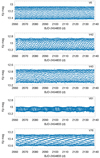 |
Fig. 1. Corrected K2 light curves of the five RRc stars that were targeted by the mission. |
One more target, M4 V75, which was identified as a possible RRc star by Yao et al. (1988), is located within the K2 custom aperture as well. This star, however, shows no periodic variation, confirming previous nondetections by Stetson et al. (2014) and Safonova et al. (2016).
2.2. Observational constraints
A detailed asteroseismic analysis requires further constraints on the physical parameters (such as L, Teff, log g or [Fe/H]) of the stars. Howell et al. (2022) used scaling relations for the red giants in the cluster, which relies on luminosities and effective temperatures. These quantities can be calculated from photometry, but they require accurate corrections for interstellar extinction. Here we used the reddening map of Alonso-García et al. (2012), but with the reddening zero point (E(B–V)0 = 0.37 mag) determined specifically for M4 by Hendricks et al. (2012).
In contrast, our approach for the RRc stars is akin to peak-bagging, where we collect and fit individual oscillation peaks (Appourchaux 2003). However, since we are limited to very few modes, it is still important to constrain our modeling space with classical observables such as allowed luminosity, Teff, and metallicity ranges.
We collected the average brightness values of the RRc stars both in Gaia DR3 passbands, and in the Johnson B and V passbands from the observations of Stetson et al. (2014, 2019)2. The Johnson data set is displayed in Fig. 2, with the RRc stars and the stars studied by Howell et al. (2022) highlighted. Although former studies by Netzel & Smolec (2022), Netzel et al. (2023) used Gaia data, here we decided to use on the Johnson brightness for consistency with the red giant analysis.
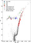 |
Fig. 2. Color-magnitude diagram of M4 in Johnson passbands using photometry from Stetson et al. (2014, 2019). The stars targeted by our study are identified by the colored star symbols; the stars in Howell et al. (2022) are shown as colored points. V6 & V42 overlap in the plot, which is indicated by the dual colored marker. The photometry has been corrected for dust using the Alonso-García et al. (2012) and Pancino et al. (2024) maps. The Gaia membership sample (gray) is from Vasiliev & Baumgardt (2021). |
We calculated the insterstellar extinction for the RRc targets similarly to that of the red giant targets, initially relying on the Alonso-García et al. (2012) and Pancino et al. (2024) differential reddening maps and the same zero point. The latter covers a larger area, but otherwise we found the two maps to be consistent with each other, with differences not exceeding ±0.02 mag. We determined extinctions for four out of five RRc stars this way. We used the zero point of Hendricks et al. (2012) here as well.
The fifth star, V43, falls outside each map. For this star, we compared the E(B–V) reddening values to the E(BP–RP) reddenings from Gaia DR3. We limited the comparison to sources with G < 15 mag, (BP–RP) < 1.4 mag, and E(BP–RP) < 1.3 mag, and cut out the core of the cluster. These filters were necessary to remove sources with very high reddenings in the catalog. This local comparison of 67 stars resulted in the conversion of E(B − V) = 0.169 E(BP − RP)+0.290. We note, however, that this formula has not been tested more extensively, and such conversions elsewhere will require further calibrations. Furthermore, the RR Lyrae variables themselves have Gaia reddenings considerably larger than their neighboring stars, so we instead calculated the median of nine neighboring stars for V43.
We then used the distance modulus provided by Baumgardt & Vasiliev (2021), μ = 11.337 ± 0.018 mag, to convert the extinction-corrected values into absolute magnitudes.
The effective temperature, Teff, was calculated using the color-Teff relation by González Hernández & Bonifacio (2009) with (V-K)0 colors. For four stars, we used the (V − K)0 color indices using K-band photometry from 2MASS (Skrutskie et al. 2006). V43 lacks K-band photometry: for that star we set the range of log Teff to 3.80 − 3.90 dex. The dereddened color (V − K)0 was calculated using the color excess E(V − K) obtained from E(B − V) with the transformation relation of Fitzpatrick & Massa (2007). The calculated ranges of Teff are collected in Table 1.
Input parameter ranges, pulsation periods, and period ratios for each RRc star that we used for modeling.
We set the metallicity to [Fe/H] ≈ − 1.1 ± 0.07 (Harris 1996; Marino et al. 2008; MacLean et al. 2018). The luminosity was calculated using the formula
 (1)
(1)
where Mbol is a bolometric brightness of a star, and Mbol⊙ is a bolometric brightness of the Sun, set to 4.74 mag. We converted MV to Mbol using the bolometric correction calculated with the relation by Alonso et al. (1999), which uses Teff and metallicity [Fe/H]. The resulting luminostiy ranges are collected in Table 1.
Metal, Z, and helium, Y, content were calculated based on [Fe/H]. First, we transformed [Fe/H] to [M/H] using the formula by Salaris et al. (1993):
![Mathematical equation: $$ \begin{aligned} \mathrm{[M/H]} \approx \mathrm{[Fe/H]} + \log \left(0.638 \cdot 10^{[\alpha /\mathrm{Fe}]} + 0.362 \right). \end{aligned} $$](/articles/aa/full_html/2025/10/aa52118-24/aa52118-24-eq2.gif) (2)
(2)
Here [α/Fe] is enhancement by α elements. Metal-poor populations have elevated α element abundances: for M4, Marino et al. (2008) found [α/Fe] = +0.39 ± 0.05 (Johnson et al. 2014; Bensby et al. 2017).
Then, we transformed [M/H] to Z, using the relation
![Mathematical equation: $$ \begin{aligned} \mathrm{[M/H]} = \log \frac{Z}{\mathrm{Z_\odot }} - \log \frac{X}{\mathrm{X_\odot }}, \end{aligned} $$](/articles/aa/full_html/2025/10/aa52118-24/aa52118-24-eq3.gif) (3)
(3)
where Z⊙ and X⊙ are solar values, which we set to Z⊙ = 0.0134 and X⊙ = 0.7381 (Asplund et al. 2009).
Assuming that hydrogen content, X, can vary from 0.70 to 0.76, and α-element enhancement can vary from 0 to 0.4, we calculated the modeling range for Z to be 0.00086–0.0032.
3. Photometric results on the RRc stars
We used the Period04 software to determine the frequency composition of each star (Lenz & Breger 2005). The detection limit was set to S/N > 4.0, relative to the nearby average noise level in the frequency spectrum. First, we subtracted the pulsation frequency and its harmonics, then searched for any extra signals above or below the pulsation frequency. Folded light curves and frequency spectra are displayed in Fig. 3.
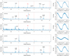 |
Fig. 3. Left: Fourier spectra of the five RRc stars. Here we removed the main pulsation frequency and its harmonics belonging to the first overtone to reveal the low-amplitude extra modes. Modes are labeled in red, and combination frequencies in black. Right: Light curves folded with the first overtone period. |
3.1. Extra modes
According to Dziembowski (2016), the signals around period ratios P/PO1 ≈ 0.63 and 0.61, relative to the first overtone, correspond to (the first harmonic of) l = 8 and l = 9 modes, respectively. Here we label these as f63 and f61 frequencies, although this family of modes is also called f61 or fX modes collectively. The actual mode frequencies are the subharmonics of these signals at f61/2 and f63/2, but those are usually harder to detect due to geometric cancellation effects.
We clearly identified the modes in four stars: V6, V42, V43, and V76. We also see subtle differences between them. In V6, the subharmonic at the true pulsation frequency is the strongest, which is unusual among RRc stars as we expect the harmonic to be stronger. In V42 and V76, we detect multiple peaks and the corresponding harmonics and subharmonics. In V43, the peak appears to be incoherent and can be fitted with three close-by frequencies. Here we observe a very wide structure at the subharmonic that extends below the expected range of the f61 modes. However, these frequencies are not low enough to be either the fundamental mode or an f68 mode.
While f61 modes are prevalent in the RRc population of M4, we did not detect the low-frequency f68 mode clearly in either of the targets. The latter is a separate group of extra modes, discovered recently in RRc stars, which appear at lower frequencies (f/fO1 ≈ 0.686), and whose origin has not been identified yet (Netzel et al. 2015c; Benkő & Kovács 2023). The lack of detection is in agreement with the mode abundance results of Netzel et al. (2024). They found that while the f61 modes are most frequent around [Fe/H] ≈ −1.0, the frequency of the f68 mode drops drastically above −1.3, and the metallicity of M4 is higher than that limit.
In contrast to the results above, V61 turned out to be the rather different from the four other stars. Here we only detect significant extra frequency peaks at the subharmonic range, but not at the expected f61 range. The two peaks appear at period ratios 0.7335 and 0.7877. The former value may potentially correspond to the fundamental mode, with a period of 0.36168 d; however, that would put the star to [Fe/H] values higher than that of M4 in the Petersen diagram (Szabó et al. 2004; Chen et al. 2023). We investigate the modulation properties of the star in Appendix A.
3.2. Petersen diagram
We present the identified f61 signals on a Petersen diagram in Fig. 4, showing the period ratios against the longer period (here fixed to the first overtone). We plot the M4 results in red against the points presented by Molnár et al. (2023a). We find that the points line up well with other samples that have moderate metallicities, such as the bulge and NGC 6362. In this regime most frequencies clearly fall onto the main ridges at period ratios P1/PX ≈ 0.632 and 0.613, corresponding to the ℓ = 8 and 9 modes. We also detect signals in the middle ridge, which Dziembowski (2016) interprets as combination frequencies. Further signals appear below, at P1/PX ≈ 0.605 which might also be combination peaks. We did not detect any ℓ = 10 peaks which should be at P1/PX ≈ 0.6 or below, according to Dziembowski (2016).
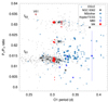 |
Fig. 4. Petersen diagram of the f61-type modes. Here we plot signals detected in M4 (in red) over the existing literature data. The frequency peaks fall onto the main ridges discovered in the OGLE data. The positions of the f61 and f63 ridges are labeled. |
3.3. Comparison with other photometric results
The K2 observations were analyzed before by Wallace et al. (2019a) who searched the cluster for new variables. They detected larger scatter in V61 than in other RR Lyrae stars, but did not recognize it as modulated. They also detected two stars they classified as millimagnitude RR Lyrae stars (Wallace et al. 2019b). Both of those two stars show only a single periodicity.
Ground-based multicolor photometry was collected for the RR Lyrae members (among others) by Stetson et al. (2014). They did not recognize V61 as a modulated star either, although upon reanalysis of their photometry, a side peak is visible. The only other star common with our targets that has a useful amount of time series photometry is V6. There a frequency signal is marginally detectable at the position of the subharmonic (f63/2). This shows that seismic modeling of RRc stars requires extensive, high-precision photometry to detect the low-amplitude extra modes.
We also analyzed the observations collected by the Zwicky Transient Facility (ZTF, Bellm et al. 2019) and the Asteroid Terrestrial-impact Last Alert System (ATLAS, Tonry et al. 2018). The ZTF data was too sparse for a detailed frequency analysis. The ATLAS survey collected significantly more data points, but the photometric precision of the observations was too low to detect any extra modes.
3.4. RRc pulsation models
For each star, we calculated pulsation models to match the observed first-overtone period and period ratio(s). To calculate the theoretical models, we used the envelope pulsation code of Dziembowski (1977). The input physical parameters required by the code are mass, luminosity, effective temperature, hydrogen and metal abundances. Additionally, this code requires an approximate value of dimensionless frequency for the nonradial mode. We followed the approach of Netzel & Smolec (2022) for individual calculations. Namely, we used the estimates that relate nonradial mode frequencies from the linear fits to sequences in the Petersen diagram (see Equations 4 and 5 in Netzel & Smolec 2022), which were then converted to dimensionless frequencies, σ, using the formula from Eq. 6 in Netzel & Smolec (2022). Furthermore, we set the range of possible starting values of nonradial mode frequencies to σ ± 0.1. Consequently, for each model we were able to get the nonradial mode with the highest driving rate, i.e., it is the most strongly trapped in the envelope.
In order to find the best matches between periods and period ratios in theoretical models and in observed values for each star, we employed genetic algorithms3, which used the pulsation code with different input physical parameters. The ranges of physical parameters were set based on observational constraints (see Table 1). In the case of mass, we set a wide range of 0.5 − 0.9 M⊙ to accommodate any realistic mass result. For each star, we executed 50 separate runs. For each run we set the maximum number of iterations to 150, population size of 100, mutation probability of 0.1, elitist ratio to 0.01, crossover probability to 0.5, and parents portion to 0.3. We note that we performed calculations with different parameters for genetic algorithms beforehand, including the numbers of populations and iterations, to ensure that the results are robust. The values and errors of physical parameters were derived as the means and standard deviations of the results from each of the fifty individual runs.
Calculated ranges of physical parameters used to constrain the models for each star are summarized in Table 1. Correlations between individual parameters based on the distributions of the results from each run are visualized with corner plots and discussed in Appendix C.
4. New and revised physical parameters
With the RRc physical parameters obtained, we proceeded to compare them to parameters of other RR Lyrae stars, as well as to the average properties of M4. For further comparison, we also recalculated the masses for the oscillating rHB stars originally studied in Howell et al. (2022).
4.1. RR Lyrae masses and other physical parameters
As listed in Table 2, the masses of four out of the five RRc stars are within 0.03 M⊙, between 0.636 and 0.667 M⊙ with an average uncertainty of ±0.031 M⊙. These masses align well with the mass-period distribution of RRc stars published by Netzel et al. (2023).
Modeled physical parameters of the five RRc stars based on seismic modeling.
The only outlier is the modulated star, V61, for which we found no solutions with unstable nonradial modes. This is caused by the higher Teff value of the star which puts it near the blue edge of the RR Lyrae instability strip, an outside of the instability region of the 0.61 modes (Netzel & Smolec 2022). This suggests that the frequency component we detected and identified tentatively as f63/2 might have a different origin. If we allow for solutions with stable modes at the detected mode frequency, we find a mass of 0.71 ± 0.05 M⊙, which is significantly higher than the rest. We include this value for the sake of completeness, but consider it as a marginal detection and do not include it in our statistics.
We compared the calculated Teff and log g values to the distribution of RR Lyrae stars presented by Molnár et al. (2023a). As Fig. 5 shows, the stars belong to the cooler RRc stars, lying between 6600–7200 K, with log g values being very close to 3.0 for all five stars. For chemical composition, we find average bulk abundances of X = 0.734 ± 0.014 and Z = 0.0016 ± 0.0005. These values indicate a He abundance of Y = 0.264 ± 0.014 for M4, pointing toward low He enrichment (ΔY < 0.02) relative to the primordial He abundance, which is in tension with the Y values inferred by Valcarce et al. (2014) spectroscopically. On the other hand, our result is in agreement with the model-based inferences of Villanova et al. (2012), supporting their conclusion that the spectroscopic data should be reevaluated, and followed upon by further observations. We note, however, that the distribution of X values among the individual model runs are skewed toward larger values for two stars (V42, V76), but are bimodal for the other two (V06 and V43) as shown in Appendix C. For V61 the fits skew toward smaller values but since it is a marginal detection we do not consider it in the averages.
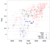 |
Fig. 5. Positions of the seismically determined Teff and log g values for the five RRc stars in M4 against the spectroscopically observed RRc stars in the Teff–log g plane, as collected by Molnár et al. (2023a). |
The comparison of the mass ratio of heavy elements, Z, to the observed [Fe/H] index is not straightforward, as it is influenced by the abundance differences of individual elements (see, e.g., Hinkel et al. 2022). Nevertheless, we can give an estimate for the correctness of our seismic Z values. Following the relations described in Section 2.2, in reverse order, and using an α-enhancement of [α/Fe] = 0.39 ± 0.05 (Marino et al. 2008), we get an average seismic [Fe/H] of −1.13 ± 0.05 for the five RRc stars, which agrees with the spectroscopic [Fe/H] value of the cluster.
4.2. Seismic masses for red giants
Mixed mode oscillations in red giants are characterized by two global seismic parameters; the large frequency separation, Δν, and the frequency of the maximum acoustic power, νmax. These quantities are correlated to stellar properties, which are used to derive seismic mass scaling relations (Ulrich 1986; Brown et al. 1991; Kjeldsen & Bedding 1995). For faint globular cluster stars, the short observing baseline of the K2 mission results in a lower frequency resolution and lower signal-to-noise ratio, and thus it can be difficult to estimate Δν. However, accurate asteroseismic masses can be measured independently of a Δν estimate (e.g., Howell et al. 2024, 2025; Reyes et al. 2025), using the following scaling relation:
 (4)
(4)
We use the oscillating red giant sample and the corresponding K2 light curves from Howell et al. (2022) to measure seismic masses using Eq. (4). They detected solar-like oscillations in 75 red giants across three phases of evolution (RGB, rHB, and early AGB), and used the pySYD pipeline (Chontos et al. 2022) to measure the asteroseismic parameters. We adopt the Howell et al. (2022) estimates for Teff and luminosity, although not their νmax measurements. Here we report updated measurements of νmax and the corresponding uncertainty for each star using a new asteroseismic pipeline, pyMON (Howell et al. 2025).
The pyMON pipeline is an adaptation of pySYD (see Chontos et al. 2022 for more details), where the main difference is that Δν is not measured. In both pipelines, the power spectrum is smoothed using an estimate for Δν; however, pyMON uses a calibrated Δν–νmax scaling relation (Stello et al. 2009) to estimate this quantity. This is useful for low signal-to-noise data – such as the M4 red giant sample in Howell et al. (2022) – where measurements are Δν are highly uncertain. A comparison between the pySYD results in Howell et al. (2022) and our pyMON results show that the measurement of νmax remains consistent; however, there is a reduction by a factor of ∼2 in the νmax uncertainty (refer to Howell et al. 2025 for further discussion on this uncertainty reduction). Consequently, this results in a decrease in the seismic mass uncertainties by a factor of ∼1.5.
Scaling relations may also include correction factors (fνmax, fΔν) to account for structural differences between the Sun and the target stars. In this case we are only interested in the value of fνmax, for which various prescriptions have been given in the literature (see, e.g., Sharma et al. 2016; Hekker 2020; Pinsonneault et al. 2025), but these have been limited to higher metallicities. More recently, Lindsay & Hon (2025) found that at the metallicity of M4, fνmax ≈ 1.05, which could indicate an overestimation of about 5% of RGB masses. However, that only applies to RGB stars, and correction factors have not been estimated for low-metallicity core-He-burning or AGB stars yet.
We note, however, that correction factors are predominantly calibrated through (or involving) stellar radii, and Ash et al. (2025) showed that radius-based fνmax values could potentially result in overcorrecting the masses. They also found that while not using any fνmax corrections can result in small systematic errors in the seismic masses, the differences stay largely constant along the RGB (and larger, νmax-dependent deviations only occur when Δν is also used). Thus, if fνmax does not depend on νmax, the mass differences between different stars will not be affected.
Furthermore, clusters offer the possibility to test the masses against stellar models and isochrones. Howell et al. (2022) found that the RGB masses agree with the masses of the fitted isochrone without the need for correction factors. We also show the agreement between our RGB masses and stellar models in Sect. 4.4. We also note that decreasing our AGB masses by 5% would be in tension with the white dwarf masses in the cluster (see Sect. 4.3). Based on these arguments, and also to stay consistent with analyses of other globular clusters which used fνmax = 1 (Howell et al. 2022, 2024, 2025), we decided to keep fνmax at unity.
4.3. Average masses of the subpopulations
Most Galactic globular clusters contain multiple populations of stars, usually signaling two consecutive waves of star formation (Milone & Marino 2022). M4 is no exception to this: the possible signs of both populations in the RGB data and their mass difference was already explored by Howell et al. (2022). However, since the RGB population showed only weak signs of bimodality at the mass, disentangling the RGB population will require further chemical abundance measurements. Since here we are more concerned about the later stages of stellar evolution, we treat the RGB sample as a single population. Using spectroscopy, MacLean et al. (2018) reported that all AGB stars in M4 belong to the first generation of stars, with second-population stars possibly skipping the AGB altogether. This suggests that the EAGB stars in Howell et al. (2022) only belong to the first generation. Most importantly, Marino et al. (2011) found that both the rHB and RR Lyrae stars of the cluster are first-population stars, and the distinct blue arm of the HB contains the second population. This makes it possible to compare their masses to each other and to the EAGB stars as well.
In Figure 6, we show the distribution of our masses as kernel density estimation (KDE) functions (top panel) and as a scatter plot (bottom panel) for each evolutionary phase. We removed the stars identified as mass outliers in Howell et al. (2022) and our study (V61). Additionally, we limited the RGB sample to below the luminosity bump (hereby known as lower RGB or LRGB) to ensure there was no bias to lower masses due to any mass loss that might have occurred. To estimate a new average mass for the rHB sample, we determine the peak value of the corresponding KDE. This represents the mode mass for this sample, and was measured to be 0.655 ± 0.007 M⊙, where the uncertainty is calculated as the standard error on the mean. Our average rHB mass is consistent with the value found previously in Howell et al. (2022). This was similarly found for the RGB and early AGB samples, where we calculated average masses of 0.80 ± 0.009 M⊙ and 0.55 ± 0.01 M⊙ respectively4. Individual and average masses relative to the calculated luminosities are plotted in Fig. 7, and are listed in Table 3.
Average masses of each evolutionary group.
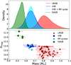 |
Fig. 6. Top: Mass distributions (calculated as KDEs) for the M4 sample of red giants and RR Lyraes, separated into evolutionary phases. For the HB sample, we include a KDE consisting of just the rHB sample (blue), and a KDE that combines both the rHB and RR Lyrae samples (cyan). We note that the area of each KDE is normalized to one, and thus the heights of the distributions do not correspond to sample sizes. Mass outliers have been removed. Bottom: Individual masses for the red giant and RR Lyrae samples plotted against Gaia magnitude. |
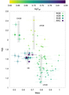 |
Fig. 7. Distribution of masses with increasing luminosity among the evolutionary groups. The lines indicate the average masses and uncertainties. |
The integrated mass loss between evolutionary phases are also consistent with Howell et al. (2022). The mass loss from the lower RGB to the HB decreases slightly to ΔMRGB − HB = 0.145 ± 0.011, whereas we find a mass loss from ΔMHB − AGB = 0.105 ± 0.013 from the HB to the early AGB.
A further mass constraint for the cluster was determined by Kalirai et al. (2009), who inferred masses of 0.50–0.55 M⊙ for six white dwarfs. As discussed by Howell et al. (2022), this is very close to the AGB seismic masses, indicating very low mass-loss on the AGB, which can be explained by the stars skipping most or all of the thermally pulsing stage of the AGB. We note that discrepancies between AGB evolutionary models and elemental abundances in the AGB stars have also been reported MacLean et al. (2018). A KDE-based fitting of the WD data, consistent with our analysis of the other populations, resulted in an average mass of  M⊙, which is lower than the average published by Kalirai et al. (2009). While this is still quite close to the EAGB mass, the difference is 0.03 M⊙, suggesting a small amount of AGB mass loss. We note, however, that the AGB mass distribution is based on only four stars, which makes the AGB average mass rather uncertain.
4.4. The seismic HRD of M4
We plot the distributions of the masses along the HRD in Fig. 8. We also include a MESA Isochrones and Stellar Tracks (MIST5; Choi et al. 2016) isochrone for comparison. This isochrone has an age of 12.2 Gyr, an average of various literature sources for M4 (Cabrera-Ziri & Conroy 2022). Since MIST does not offer α-enhanced isochrones, we use a value of [Fe/H] = –0.9 to emulate the higher [α/Fe] abundances, based on the scaling described by Joyce et al. (2023). The mass loss prescriptions used by MIST for low-mass stars are ηR = 0.1 and ηB = 0.2 for the RGB and AGB phases, following the Reimers (1975) and Bloecker (1995) schemes, respectively. Colors represent masses: it is clear that the conservative mass loss prescription used in MIST’s pre-computed isochrone database does not capture the true amount of mass loss in the cluster. This is most evident in the later evolutionary stages.
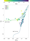 |
Fig. 8. Seismic HRD of M4. Here we show stars in the log L − Teff plane for which masses are available. The colors indicate stellar mass. The gap in the HB between RRc and rHB stars is where RRab stars reside and for which no mass estimate is available. The solid line is a MIST isochrone with an age of 12.2 Gyr and an [Fe/H] index of –0.9. Two BaSTI ZAHB tracks ([α/Fe] = 0.4; [Fe/H] = –0.9 (lower) and [Fe/H] = –1.2 (upper) are also shown. |
The isochrone has masses around 0.82–0.83 M⊙ in the RGB, which agrees with our inferred LRGB masses to within 3%, even without further optimization of the isochrone fit. We note that this again indicates that no correction is necessary for the scaling relation, since literature fνmax values would decrease the seismic masses. However, the isochrone mass only drops to 0.79 M⊙ by the time of the HB and early AGB, which is significantly higher than the observed values. A consequence of the overly conservative mass loss prescription is that the isochrone barely reaches the red edge of the rHB region and therefore cannot reproduce the structure of the HB at all. We note that mass loss parameters cannot be adjusted in MIST through the web interface, either.
Our results indicate that for old, low-mass stellar populations, such as globular clusters, pre-packaged MIST isochrones (and any other isochrone set with similarly conservative mass loss prescriptions) can only reliably reproduce the masses of stars up to the lower RGB, before reaching the red giant branch bump. This highlights the importance of cluster seismology and realistic mass loss estimates, because these studies can provide the first observational constraints on the required level of mass loss through the later stages of low-mass stellar evolution.
In order to capture the structure of the HB, we also included two zero-age horizontal branch (ZAHB) tracks in Fig. 8 from the Bag of Stellar Tracks and Isochrones (BaSTI) model library (Pietrinferni et al. 2021). Both tracks use alpha-element enhanced models ([α/Fe] = 0.4). The two pre-computed tracks closest to the [Fe/H] index of M4 have indices of –0.9 and –1.2, respectively. We also tested alpha-enhanced BaSTI isochrones at the same age as the MIST one in the plot, but they only differed significantly from MIST at the main sequence turnoff and were nearly indistinguishable along the giant branch.
4.5. Comparison of the rHB and RRc masses
As we discussed in Section 1, estimating the masses of RR Lyrae stars in a model-independent way is an extremely difficult task. While evolutionary models can be used to constrain HB masses in globular clusters (see, e.g., Gratton et al. 2010; Howell et al. 2024; Kumar et al. 2024), and masses for RRd stars can be estimated from nonlinear models (Molnár et al. 2015b), these approaches still need independent verification. Here we present, for the first time, simultaneous mass estimates based on two independent seismic approaches for stars along the HB in a globular cluster. And although these seismic models and scaling relations could still contain their own model uncertainties, they can now be verified against each other.
For M4, we found a combined HB mass of 0.652 ± 0.022 M⊙. If we split this sample into their constituent RR Lyrae and rHB parts, we find average masses of MrHB = 0.657 ± 0.034 M⊙ and MRRc = 0.648 ± 0.028 M⊙, respectively. The small difference of ≈0.01 M⊙ is in agreement with the evolutionary predictions that stellar (envelope) masses along the HB decrease toward the blue (Salaris & Cassisi 2006). Therefore, we can conclude that our two seismic mass estimates, the scaling relations for rHB stars, and the linear RRc model method of Netzel & Smolec (2022), are in agreement. Thus, we may conclude that fitting the f61 modes offers a reliable way to estimate RR Lyrae star masses, even if it is only available for overtone stars.
4.6. Comparison with mass relations and models
Relations to calculate masses for RR Lyrae, or more broadly for HB stars from observational constraints, have been given by multiple authors, derived from pulsation and evolutionary models. Here we compare seven prescriptions with our seismic masses. The first widely adopted relation on dependence of the pulsation period on the physical parameters (M, L,Teff) was published by van Albada & Baker (1971). This was later refined and updated by multiple authors, also incorporating a metallicity term (Bono et al. 1997; Jurcsik 1998; Marconi et al. 2003; Di Criscienzo et al. 2004; Marconi et al. 2015). A more general relation between mass, color, and metallicity was given for HB stars by Gratton et al. (2010).
The accuracy of these prescriptions, however, strongly depends on the modeling choices and uncertainties intrinsic to parameter choices, which are not often explored. Furthermore, many prescriptions are based on Teff and L values, which have to be converted from observations and have many uncertainties and potential parameter degeneracies themselves. Converting apparent brightness to theoretical luminosity, for example, involves uncertainties in the distance of the object, in the amount of interstellar absorption between the observer and the object, and even in the calculation of the bolometric correction. Similarly, converting observed colors to Teff involves uncertainties coming from interstellar absorption and the choice of extinction law parameter, as well as from the accuracy of the calibration of the color–Teff conversion scales themselves.
With these limitations in mind, we calculated the RR Lyrae masses using these relations and compared them to our seismic results in two ways. First we used the classical constraints, L and Teff values, computed from the Johnson photometry, which also served as initial values for our seismic model fits. These results are plotted in the left panel of Fig. 9. As the figure shows, the values are generally in the right range, between 0.45 and 1.0 M⊙; however, differences from the seismic values can reach 0.1–0.3 M⊙.
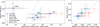 |
Fig. 9. Comparison of the RRc masses with results from various mass relations based on physical parameters. Left: Masses calculated from classical observational constraints obtained for L and Teff. Right: Masses calculated from the L and Teff outputs produced by our seismic results listed in Table 2. The seismic masses are shifted by small amounts in both plots to make the individual error bars visible. The dashed line is the identity line in both plots. |
We then recalculated the masses using the L and Teff values obtained from the seismic model fits listed in Table 2, and plotted them in the right panel of Fig. 9. In contrast with the results above, these correlate very well with our seismic masses. The matches are not perfect, however, as clear systematic differences are visible. Most relations give results very similar to the original one published by van Albada & Baker (1971), underestimating the masses by an average difference of –0.020 to –0.028 M⊙, relative to the seismic masses. The only relation that overestimates the masses is that of Marconi et al. (2015), with an average difference of +0.032 M⊙. These results highlight the true difference between various models and their parameter choices, rather than the uncertainties coming from the observations. The main source of observational uncertainty left in these fits is in the frequencies of the modes we fit.
Gratton et al. (2010) determined a different mass relation based on the B − V (or V − I) color indices and [Fe/H] indices of HB stars. We calculated the masses of both the RRc and the rHB stars using our dereddened B − V colors. The results are displayed in Fig. 10. This relation results in a higher mass difference (0.037 M⊙) between the two groups than what we found from the seismic data. This difference could be related to he fact that the relation is based on zero-age HB stellar models, whereas the stars in M4 are not necessarily on the ZAHB, but rather at evolutionary stages dictated by their common ages and thus common masses.
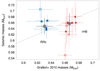 |
Fig. 10. Comparison of the seismic HB masses, both for the RRc and rHB stars, with the mass relation published by Gratton et al. (2010). The empty symbols indicate marginal detections. The large gray symbols indicate the averages for both groups. The dashed line is the identity line. |
Finally, we compared our results directly to the BaSTI ZAHB models. We plot three model sequences in Fig. 11 on the log(Teff) – mass plane. All three models are α-enhanced ([α/Fe] = +0.4), with differing [Fe/H] indices (−1.3, −1.2, −0.9) but similar He content (Y = 0.259, 0.250, 0.252). While the inferred mass and Teff values do not line up well with a single track, three out of four RRc stars within 1σ from the measured [Fe/H] = −1.1 ± 0.07 value of the cluster, with RRc stars aligning with slightly more metal-poor (more massive), and RHB stars with slighly metal-rich (lighter) sequences. This result agrees with what we observe in Fig. 10. However, whether the ZAHB models overestimate the mass gradient along the HB or our mass measurements contain systematic offsets cannot be decided from these results alone.
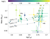 |
Fig. 11. Comparison of the seismic HB masses to the BaSTI ZAHB model sequences. All three models are α-enhanced ([α/Fe] = 0.4), and have similar He abundances, but differing metal content. The colors indicate luminosities; the squares represent RRc stars and the circles represent RHB stars; the empty symbols indicate marginal detections. |
5. Conclusions
Determining the masses of RR Lyrae variables is a notoriously difficult task. While relations based on physical parameters exist, and pulsational masses can, in principle, provide masses for double-mode stars, these are strongly model-dependent methods that could not be verified by independent mass estimates. Asteroseismology offers a new way to determine stellar masses (Aerts 2021). While seismic masses still depend on stellar envelope models and on the validity of scaling relations, they can be tested against other observational techniques (e.g., dynamical masses in eclipsing binaries).
Globular clusters, such as M4, provide an opportunity to probe the late stages of low-mass stellar evolution. Building on the unique capabilities of the Kepler space telescope, we calculated new, more accurate masses for the oscillating giant stars using asteroseismic scaling relations and νmax values determined with the new pyMON code (Howell et al., in prep.). We then analyzed the overtone RR Lyrae stars in the cluster and determined their masses via peak-bagging and fitting the frequencies with seismic model calculations Netzel & Smolec (2022), Netzel et al. (2023). With these, we were able to relate RR Lyrae seismic masses to seismic masses of red HB stars, and found that they match each other closely, with the RR Lyrae models being lighter, as expected from stellar evolution. We found the average rHB and RRc masses to be MrHB = 0.657 ± 0.034 M⊙ and MRRc = 0.648 ± 0.028 M⊙, respectively.
Furthermore, we estimate a low He enrichment in the cluster, in agreement with the findings of Villanova et al. (2012), based on the RRc model results. However, the models leave the chemical compositions ambiguous for multiple targets, which makes this result uncertain.
While our result is not yet a direct measurement of RR Lyrae masses, as it relies on the assumption that RR Lyrae and rHB stars in the cluster have very similar masses, we were able to test model-dependent seismic (or pulsational) masses against independent mass estimates for the first time. We find that while the RRc stars have slightly lower masses, as expected from the stucture of the HB, the difference of ≈0.01 M⊙ is less than what stellar evolutionary models predict. Whether the source of this discrepancy comes from the pulsational or the evolutionary models remains to be seen: but even if considering such systematic differences, we estimate that our method to determine RR Lyrae masses is accurate to σM ≈ 0.05 M⊙.
We also compared the modeled physical parameters of the RRc stars to various relations between M, L, Teff, and the pulsation periods, and found that while these generally agree, systematical differences do exist. We also show, however, that the usability of these relations is rather limited, as L and Teff values have to be determined very accurately, otherwise the calculated masses will be very uncertain.
This study not only tests RR Lyrae masses for the first time, but it also lends further support to the hypothesis of the f61 modes being high-order ℓ modes, as proposed by Dziembowski (2016). Therefore, it is now possible to estimate masses (and log g values) for field RRc and RRd stars to within a few hundredth M⊙ accuracy, if enough modes can be detected from high-precision photometry (Netzel & Smolec 2022; Netzel et al. 2023). Furthermore, RRc stars now offer a way to measure masses on the HB in globular clusters, even where rHB stars are too faint for asteroseismology. RR Lyrae stars thus open up a new way to study mass loss in more clusters, either with Kepler (Kalup et al., in prep.) or with future instruments, such as the Roman Space Telescope (Molnár et al. 2023b) or the HAYDN telescope project, which is designed specifically to observe dense stellar fields (Miglio et al. 2021).
Data availability
Full Table C.1 is available at the CDS via https://cdsarc.cds.unistra.fr/viz-bin/cat/J/A+A/702/A116
Ms. Tseraskaya (Ceraski) collected the data at Moscow Observatory that led to the discovery.
We used a Python geneticlagorithm library https://github.com/rmsolgi/geneticalgorithm
We highlight that Howell et al. (2022) used the mean mass as their average mass scale. In this paper, we adopt the same method as Howell et al. (2024) of measuring the mode mass of the KDE distributions to determine the average mass. Both average mass measures are consistent within uncertainties.
Acknowledgments
This research was supported by the ‘SeismoLab’ KKP-137523 Élvonal grant and the NKFIH excellence grant TKP2021-NKTA-64 of the Hungarian Research, Development and Innovation Office (NKFIH), and by the LP2025-14/2025 Lendület grant of the Hungarian Academy of Sciences. Cs.K. was supported by the EKÖ?P-24 University Excellence Scholarship Program of the Ministry for Culture and Innovation, financed by the National Research, Development and Innovation Fund. This research has received support from the European Research Council (ERC) under the European Union’s Horizon 2020 research and innovation programme (Grant Agreement No. 947660). H.N. is funded by the Swiss National Science Foundation (award PCEFP2_194638) and the European Research Council (ERC) under the European Union’s Horizon 2020 research and innovation program (grant agreement No. 951549 – UniverScale). M.J. gratefully acknowledges funding of MATISSE: Measuring Ages Through Isochrones, Seismology, and Stellar Evolution, awarded through the European Commission’s Widening Fellowship. This project has received funding from the European Union’s Horizon 2020 research and innovation programme. This research made use of NASA’s Astrophysics Data System Bibliographic Services, as well as of the SIMBAD database operated at CDS, Strasbourg, France.
References
- Abdollahi, H., Molnár, L., & Varga, V. 2025, A&A, 695, L14 [NASA ADS] [CrossRef] [EDP Sciences] [Google Scholar]
- Aerts, C. 2021, Rev. Mod. Phys., 93, 015001 [Google Scholar]
- Aigrain, S., Parviainen, H., & Pope, B. J. S. 2016, MNRAS, 459, 2408 [NASA ADS] [Google Scholar]
- Alonso, A., Arribas, S., & Martínez-Roger, C. 1999, A&AS, 140, 261 [NASA ADS] [CrossRef] [EDP Sciences] [Google Scholar]
- Alonso-García, J., Mateo, M., Sen, B., et al. 2012, AJ, 143, 70 [Google Scholar]
- Anders, E. H., & Pedersen, M. G. 2023, Galaxies, 11, 56 [NASA ADS] [CrossRef] [Google Scholar]
- Antipin, S. V., & Jurcsik, J. 2005, Inf. Bull. Variable Stars, 5632, 1 [Google Scholar]
- Appourchaux, T. 2003, Ap&SS, 284, 109 [Google Scholar]
- Ash, A. L., Pinsonneault, M. H., Vrard, M., & Zinn, J. C. 2025, ApJ, 979, 135 [Google Scholar]
- Asplund, M., Grevesse, N., Sauval, A. J., & Scott, P. 2009, ARA&A, 47, 481 [NASA ADS] [CrossRef] [Google Scholar]
- Barnes, T. G., Guggenberger, E., & Kolenberg, K. 2021, AJ, 162, 117 [Google Scholar]
- Baumgardt, H., & Vasiliev, E. 2021, MNRAS, 505, 5957 [NASA ADS] [CrossRef] [Google Scholar]
- Bellinger, E. P., Kanbur, S. M., Bhardwaj, A., & Marconi, M. 2020, MNRAS, 491, 4752 [NASA ADS] [CrossRef] [Google Scholar]
- Bellm, E. C., Kulkarni, S. R., Graham, M. J., et al. 2019, PASP, 131, 018002 [Google Scholar]
- Benkő, J. M., & Kovács, G. B. 2023, A&A, 680, L6 [NASA ADS] [CrossRef] [EDP Sciences] [Google Scholar]
- Bensby, T., Feltzing, S., Gould, A., et al. 2017, A&A, 605, A89 [NASA ADS] [CrossRef] [EDP Sciences] [Google Scholar]
- Blažko, S. 1907, Astron. Nachr., 175, 325 [Google Scholar]
- Bloecker, T. 1995, A&A, 297, 727 [Google Scholar]
- Bobrick, A., Iorio, G., Belokurov, V., et al. 2024, MNRAS, 527, 12196 [Google Scholar]
- Bódi, A., Szabó, P., Plachy, E., Molnár, L., & Szabó, R. 2022, PASP, 134, 014503 [CrossRef] [Google Scholar]
- Bono, G., Caputo, F., Castellani, V., & Marconi, M. 1997, A&AS, 121, 327 [NASA ADS] [CrossRef] [EDP Sciences] [Google Scholar]
- Brown, T. M., Gilliland, R. L., Noyes, R. W., & Ramsey, L. W. 1991, ApJ, 368, 599 [Google Scholar]
- Cabrera-Ziri, I., & Conroy, C. 2022, MNRAS, 511, 341 [NASA ADS] [CrossRef] [Google Scholar]
- Catelan, M. 2009, Ap&SS, 320, 261 [Google Scholar]
- Chen, X., Zhang, J., Wang, S., & Deng, L. 2023, Nat. Astron., 7, 1081 [Google Scholar]
- Choi, J., Dotter, A., Conroy, C., et al. 2016, ApJ, 823, 102 [Google Scholar]
- Chontos, A., Huber, D., Sayeed, M., & Yamsiri, P. 2022, J. Open Source Software, 7, 3331 [Google Scholar]
- Cruz Reyes, M., Anderson, R. I., Johansson, L., Netzel, H., & Medaric, Z. 2024, A&A, 684, A173 [NASA ADS] [CrossRef] [EDP Sciences] [Google Scholar]
- Das, S., Molnár, L., Kovács, G. B., et al. 2025, A&A, 694, A255 [NASA ADS] [CrossRef] [EDP Sciences] [Google Scholar]
- Di Criscienzo, M., Marconi, M., & Caputo, F. 2004, ApJ, 612, 1092 [Google Scholar]
- Dziembowski, W. 1977, Acta Astron., 27, 95 [NASA ADS] [Google Scholar]
- Dziembowski, W. A. 2016, Commmun. Konkoly Obs. Hungary, 105, 23 [NASA ADS] [Google Scholar]
- Fitzpatrick, E. L., & Massa, D. 2007, ApJ, 663, 320 [Google Scholar]
- Gaia Collaboration (Brown, A. G. A., et al.) 2021, A&A, 649, A1 [NASA ADS] [CrossRef] [EDP Sciences] [Google Scholar]
- González Hernández, J. I., & Bonifacio, P. 2009, A&A, 497, 497 [Google Scholar]
- Gratton, R. G., Carretta, E., Bragaglia, A., Lucatello, S., & D’Orazi, V. 2010, A&A, 517, A81 [CrossRef] [EDP Sciences] [Google Scholar]
- Hajdu, G., Catelan, M., Jurcsik, J., et al. 2015, MNRAS, 449, L113 [NASA ADS] [CrossRef] [Google Scholar]
- Hajdu, G., Pietrzyński, G., Jurcsik, J., et al. 2021, ApJ, 915, 50 [NASA ADS] [CrossRef] [Google Scholar]
- Harris, W. E. 1996, AJ, 112, 1487 [Google Scholar]
- Hekker, S. 2020, Front. Astron. Space Sci., 7, 3 [NASA ADS] [CrossRef] [Google Scholar]
- Hendricks, B., Stetson, P. B., VandenBerg, D. A., & Dall’Ora, M. 2012, AJ, 144, 25 [NASA ADS] [CrossRef] [Google Scholar]
- Hinkel, N. R., Young, P. A., & Wheeler, I., C. H. 2022, AJ, 164, 256 [Google Scholar]
- Howell, M., Campbell, S. W., Stello, D., & De Silva, G. M. 2022, MNRAS, 515, 3184 [NASA ADS] [CrossRef] [Google Scholar]
- Howell, M., Campbell, S. W., Stello, D., & De Silva, G. M. 2024, MNRAS, 527, 7974 [Google Scholar]
- Howell, M., Campbell, S. W., Kalup, C., Stello, D., & De Silva, G. M. 2025, MNRAS, 536, 1389 [Google Scholar]
- Johnson, C. I., Rich, R. M., Kobayashi, C., Kunder, A., & Koch, A. 2014, AJ, 148, 67 [Google Scholar]
- Joyce, M., & Tayar, J. 2023, Galaxies, 11, 75 [NASA ADS] [CrossRef] [Google Scholar]
- Joyce, M., Johnson, C. I., Marchetti, T., et al. 2023, ApJ, 946, 28 [NASA ADS] [CrossRef] [Google Scholar]
- Joyce, M., Molnár, L., Cinquegrana, G., et al. 2024, ApJ, 971, 186 [Google Scholar]
- Jurcsik, J. 1998, A&A, 333, 571 [NASA ADS] [Google Scholar]
- Kalirai, J. S., Saul Davis, D., Richer, H. B., et al. 2009, ApJ, 705, 408 [CrossRef] [Google Scholar]
- Kalup, C. E., Molnár, L., Kiss, C., et al. 2021, ApJS, 254, 7 [NASA ADS] [CrossRef] [Google Scholar]
- Karczmarek, P., Wiktorowicz, G., Iłkiewicz, K., et al. 2017, MNRAS, 466, 2842 [CrossRef] [Google Scholar]
- Kennedy, C. R., Stancliffe, R. J., Kuehn, C., et al. 2014, ApJ, 787, 6 [Google Scholar]
- Kjeldsen, H., & Bedding, T. R. 1995, A&A, 293, 87 [NASA ADS] [Google Scholar]
- Kovács, G. B., Nuspl, J., & Szabó, R. 2023, MNRAS, 521, 4878 [CrossRef] [Google Scholar]
- Kumar, N., Bhardwaj, A., Singh, H. P., et al. 2024, MNRAS, 531, 2976 [NASA ADS] [CrossRef] [Google Scholar]
- Kurtz, D. W. 2022, ARA&A, 60, 31 [NASA ADS] [CrossRef] [Google Scholar]
- Lenz, P., & Breger, M. 2005, Commun. Asteroseismol., 146, 53 [Google Scholar]
- Lindsay, C. J., & Hon, M. 2025, ApJ, 989, 189 [Google Scholar]
- Liška, J., Skarka, M., Zejda, M., Mikulášek, Z., & de Villiers, S. N. 2016a, MNRAS, 459, 4360 [NASA ADS] [CrossRef] [Google Scholar]
- Liška, J., Skarka, M., Mikulášek, Z., Zejda, M., & Chrastina, M. 2016b, A&A, 589, A94 [CrossRef] [EDP Sciences] [Google Scholar]
- MacLean, B. T., Campbell, S. W., Amarsi, A. M., et al. 2018, MNRAS, 481, 373 [Google Scholar]
- Marconi, M., Caputo, F., Di Criscienzo, M., & Castellani, M. 2003, ApJ, 596, 299 [Google Scholar]
- Marconi, M., Coppola, G., Bono, G., et al. 2015, ApJ, 808, 50 [Google Scholar]
- Marconi, M., Bono, G., Pietrinferni, A., et al. 2018, ApJ, 864, L13 [Google Scholar]
- Marino, A. F., Villanova, S., Piotto, G., et al. 2008, A&A, 490, 625 [NASA ADS] [CrossRef] [EDP Sciences] [Google Scholar]
- Marino, A. F., Villanova, S., Milone, A. P., et al. 2011, ApJ, 730, L16 [NASA ADS] [CrossRef] [Google Scholar]
- Matteuzzi, M., Montalbán, J., Miglio, A., et al. 2023, A&A, 671, A53 [NASA ADS] [CrossRef] [EDP Sciences] [Google Scholar]
- Miglio, A., Chaplin, W. J., Brogaard, K., et al. 2016, MNRAS, 461, 760 [NASA ADS] [CrossRef] [Google Scholar]
- Miglio, A., Girardi, L., Grundahl, F., et al. 2021, Exp. Astron., 51, 963 [NASA ADS] [CrossRef] [Google Scholar]
- Milone, A. P., & Marino, A. F. 2022, Universe, 8, 359 [NASA ADS] [CrossRef] [Google Scholar]
- Molnár, L., Szabó, R., Moskalik, P. A., et al. 2015a, MNRAS, 452, 4283 [CrossRef] [Google Scholar]
- Molnár, L., Pál, A., Plachy, E., et al. 2015b, ApJ, 812, 2 [Google Scholar]
- Molnár, L., Pál, A., Sárneczky, K., et al. 2018, ApJS, 234, 37 [CrossRef] [Google Scholar]
- Molnár, L., Plachy, E., Bódi, A., et al. 2023a, A&A, 678, A104 [NASA ADS] [CrossRef] [EDP Sciences] [Google Scholar]
- Molnár, L., Kalup, C., Joyce, M., et al. 2023b, ArXiv e-prints [arXiv:2306.12459] [Google Scholar]
- Nemec, J. M., Smolec, R., Benkő, J. M., et al. 2011, MNRAS, 417, 1022 [NASA ADS] [CrossRef] [Google Scholar]
- Netzel, H., & Smolec, R. 2019, MNRAS, 487, 5584 [NASA ADS] [CrossRef] [Google Scholar]
- Netzel, H., & Smolec, R. 2022, MNRAS, 515, 3439 [NASA ADS] [CrossRef] [Google Scholar]
- Netzel, H., Smolec, R., & Moskalik, P. 2015a, MNRAS, 447, 1173 [NASA ADS] [CrossRef] [Google Scholar]
- Netzel, H., Smolec, R., & Moskalik, P. 2015b, MNRAS, 453, 2022 [Google Scholar]
- Netzel, H., Smolec, R., & Dziembowski, W. 2015c, MNRAS, 451, L25 [NASA ADS] [CrossRef] [Google Scholar]
- Netzel, H., Molnár, L., & Joyce, M. 2023, MNRAS, 525, 5378 [NASA ADS] [CrossRef] [Google Scholar]
- Netzel, H., Varga, V., Szabó, R., Smolec, R., & Plachy, E. 2024, A&A, 692, A133 [NASA ADS] [CrossRef] [EDP Sciences] [Google Scholar]
- Pál, A. 2012, MNRAS, 421, 1825 [Google Scholar]
- Pancino, E., Zocchi, A., Rainer, M., et al. 2024, A&A, 686, A283 [NASA ADS] [CrossRef] [EDP Sciences] [Google Scholar]
- Pietrinferni, A., Hidalgo, S., Cassisi, S., et al. 2021, ApJ, 908, 102 [NASA ADS] [CrossRef] [Google Scholar]
- Pietrzyński, G., Thompson, I. B., Gieren, W., et al. 2012, Nature, 484, 75 [CrossRef] [Google Scholar]
- Pinsonneault, M. H., Zinn, J. C., Tayar, J., et al. 2025, ApJS, 276, 69 [NASA ADS] [CrossRef] [Google Scholar]
- Plachy, E., Molnár, L., Bódi, A., et al. 2019, ApJS, 244, 32 [CrossRef] [Google Scholar]
- Reimers, D. 1975, Mem. Soc. Roy. Sci. Liege, 8, 369 [Google Scholar]
- Reyes, C., Stello, D., Hon, M., et al. 2025, MNRAS, 538, 1720 [Google Scholar]
- Riello, M., De Angeli, F., Evans, D. W., et al. 2021, A&A, 649, A3 [NASA ADS] [CrossRef] [EDP Sciences] [Google Scholar]
- Safonova, M., Mkrtichian, D., Hasan, P., et al. 2016, AJ, 151, 27 [Google Scholar]
- Salaris, M., & Cassisi, S. 2006, Evolution of Stars and Stellar Populations (Wiley) [Google Scholar]
- Salaris, M., Chieffi, A., & Straniero, O. 1993, ApJ, 414, 580 [NASA ADS] [CrossRef] [Google Scholar]
- Shapley, H. 1916, ApJ, 43, 217 [Google Scholar]
- Sharma, S., Stello, D., Bland-Hawthorn, J., Huber, D., & Bedding, T. R. 2016, ApJ, 822, 15 [Google Scholar]
- Skrutskie, M. F., Cutri, R. M., Stiening, R., et al. 2006, AJ, 131, 1163 [NASA ADS] [CrossRef] [Google Scholar]
- Smolec, R., & Moskalik, P. 2008, Acta Astron., 58, 193 [NASA ADS] [Google Scholar]
- Smolec, R., Moskalik, P., Kałużny, J., et al. 2017, MNRAS, 467, 2349 [NASA ADS] [Google Scholar]
- Stello, D., Chaplin, W. J., Basu, S., Elsworth, Y., & Bedding, T. R. 2009, MNRAS, 400, L80 [Google Scholar]
- Stetson, P. B., Braga, V. F., Dall’Ora, M., et al. 2014, PASP, 126, 521 [NASA ADS] [CrossRef] [Google Scholar]
- Stetson, P. B., Pancino, E., Zocchi, A., Sanna, N., & Monelli, M. 2019, MNRAS, 485, 3042 [Google Scholar]
- Sylla, S., Kolenberg, K., Klotz, A., et al. 2024, A&A, 691, A108 [NASA ADS] [CrossRef] [EDP Sciences] [Google Scholar]
- Szabó, R., Kolláth, Z., & Buchler, J. R. 2004, A&A, 425, 627 [NASA ADS] [CrossRef] [EDP Sciences] [Google Scholar]
- Tailo, M., Corsaro, E., Miglio, A., et al. 2022, A&A, 662, L7 [NASA ADS] [CrossRef] [EDP Sciences] [Google Scholar]
- Tonry, J. L., Denneau, L., Heinze, A. N., et al. 2018, PASP, 130, 064505 [Google Scholar]
- Ulrich, R. K. 1986, ApJ, 306, L37 [Google Scholar]
- Valcarce, A. A. R., & Catelan, M. 2008, A&A, 487, 185 [NASA ADS] [CrossRef] [EDP Sciences] [Google Scholar]
- Valcarce, A. A. R., Catelan, M., Alonso-García, J., Cortés, C., & De Medeiros, J. R. 2014, ApJ, 782, 85 [NASA ADS] [CrossRef] [Google Scholar]
- van Albada, T. S., & Baker, N. 1971, ApJ, 169, 311 [NASA ADS] [CrossRef] [Google Scholar]
- Vasiliev, E., & Baumgardt, H. 2021, MNRAS, 505, 5978 [NASA ADS] [CrossRef] [Google Scholar]
- Villanova, S., Geisler, D., Piotto, G., & Gratton, R. G. 2012, ApJ, 748, 62 [NASA ADS] [CrossRef] [Google Scholar]
- Wade, R. A., Donley, J., Fried, R., White, R. E., & Saha, A. 1999, AJ, 118, 2442 [NASA ADS] [CrossRef] [Google Scholar]
- Wallace, J. J., Hartman, J. D., Bakos, G. Á., & Bhatti, W. 2019a, ApJS, 244, 12 [NASA ADS] [CrossRef] [Google Scholar]
- Wallace, J. J., Hartman, J. D., Bakos, G. Á., & Bhatti, W. 2019b, ApJ, 870, L7 [NASA ADS] [CrossRef] [Google Scholar]
- Yao, B. A., Tong, J. H., & Zhang, C. S. 1988, Acta Astron. Sin., 29, 243 [Google Scholar]
Appendix A: V61, the modulated star
The light curve of V61 has a much lower pulsation amplitude compared to the others and shows amplitude and phase modulations. This pattern is very similar to the modulated low-amplitude RRc stars observed in M80 Molnár et al. (2023a) and elsewhere (Antipin & Jurcsik 2005; Smolec et al. 2017; Netzel & Smolec 2019). Just like in those cases, we detect asymmetry side peaks next to the pulsation frequency, in this case, above it. We cut the light curve into 1.5 d long segments and fitted A1 and ϕ1 for each segment separately with the same, fixed f1 frequency to study the shape of the modulation more closely.
As Figure C.1 shows, the modulation pattern is multiperiodic. We calculated the Fourier-spectra of both the amplitude and phase variations. The former is also shown in Fig. C.1; the spectrum of the phase variation looks very similar. Both show to separate frequency peak, from which we calculated two modulation periods: Pm1 = 11.39 ± 0.05 d and Pm2 = 19.63 ± 0.25 d.
Appendix B: Data tables
In Table C.1, we present the reduced K2 light curves for the five RRc stars analyzed in this work. The full table will be available online. In Table C.4, we list the updated seismic and physical parameters for the RGB, AGB, and rHB stars. In Tables C.2 and C.3 we list the mass estimates we show in Figures 9 and 10.
Appendix C: Corner plots
The corner plots for each RRc star are shown in Figs. C.2, C.3, C.4, C.5, and C.6, respectively. The diagonal panels display histograms of the parameter distributions, with vertical lines indicating the mean values and their associated uncertainties, which are also annotated at the top of each column. The peak of the mass distribution generally coincides with its mean value. Interestingly, the distribution of the hydrogen content X shows bimodality, where two distinct maxima appear at the boundaries of the accepted range. This effect is most pronounced for V06 and V42.
Several parameter correlations are evident. As expected, there is a clear positive correlation between effective temperature and luminosity, which follows the lines of constant period. Additionally, for V06 and V42, an anticorrelation between effective temperature and mass, as well as between luminosity and mass is visible. This is also expected as mass and effective temperature are anticorrelated along the HB.
K2SC-corrected and trend-corrected photometric data for the five RRc stars. The full table is available in machine-readable format at the CDS.
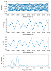 |
Fig. C.1. V61 amplitude and phase modulation |
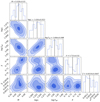 |
Fig. C.2. Corner plot for V06. The solid and dashed black lines in the diagonal panels correspond to the mean values and their standard deviation, as indicated at the top of each column. |
Mass values for RR Lyrae and rHB stars based on the mass relation of Gratton et al. (2010), compared to our seismic masses.
Mass values calculated from the various mass relations, using either the classical observational constraints or the physical parameters from our seismic fits as constraints.
The updated global seismic properties and calculated physical parameters for the giants in M4.
All Tables
Input parameter ranges, pulsation periods, and period ratios for each RRc star that we used for modeling.
K2SC-corrected and trend-corrected photometric data for the five RRc stars. The full table is available in machine-readable format at the CDS.
Mass values for RR Lyrae and rHB stars based on the mass relation of Gratton et al. (2010), compared to our seismic masses.
Mass values calculated from the various mass relations, using either the classical observational constraints or the physical parameters from our seismic fits as constraints.
The updated global seismic properties and calculated physical parameters for the giants in M4.
All Figures
|
Fig. 1. Corrected K2 light curves of the five RRc stars that were targeted by the mission. |
| In the text | |
|
Fig. 2. Color-magnitude diagram of M4 in Johnson passbands using photometry from Stetson et al. (2014, 2019). The stars targeted by our study are identified by the colored star symbols; the stars in Howell et al. (2022) are shown as colored points. V6 & V42 overlap in the plot, which is indicated by the dual colored marker. The photometry has been corrected for dust using the Alonso-García et al. (2012) and Pancino et al. (2024) maps. The Gaia membership sample (gray) is from Vasiliev & Baumgardt (2021). |
| In the text | |
|
Fig. 3. Left: Fourier spectra of the five RRc stars. Here we removed the main pulsation frequency and its harmonics belonging to the first overtone to reveal the low-amplitude extra modes. Modes are labeled in red, and combination frequencies in black. Right: Light curves folded with the first overtone period. |
| In the text | |
|
Fig. 4. Petersen diagram of the f61-type modes. Here we plot signals detected in M4 (in red) over the existing literature data. The frequency peaks fall onto the main ridges discovered in the OGLE data. The positions of the f61 and f63 ridges are labeled. |
| In the text | |
|
Fig. 5. Positions of the seismically determined Teff and log g values for the five RRc stars in M4 against the spectroscopically observed RRc stars in the Teff–log g plane, as collected by Molnár et al. (2023a). |
| In the text | |
|
Fig. 6. Top: Mass distributions (calculated as KDEs) for the M4 sample of red giants and RR Lyraes, separated into evolutionary phases. For the HB sample, we include a KDE consisting of just the rHB sample (blue), and a KDE that combines both the rHB and RR Lyrae samples (cyan). We note that the area of each KDE is normalized to one, and thus the heights of the distributions do not correspond to sample sizes. Mass outliers have been removed. Bottom: Individual masses for the red giant and RR Lyrae samples plotted against Gaia magnitude. |
| In the text | |
|
Fig. 7. Distribution of masses with increasing luminosity among the evolutionary groups. The lines indicate the average masses and uncertainties. |
| In the text | |
|
Fig. 8. Seismic HRD of M4. Here we show stars in the log L − Teff plane for which masses are available. The colors indicate stellar mass. The gap in the HB between RRc and rHB stars is where RRab stars reside and for which no mass estimate is available. The solid line is a MIST isochrone with an age of 12.2 Gyr and an [Fe/H] index of –0.9. Two BaSTI ZAHB tracks ([α/Fe] = 0.4; [Fe/H] = –0.9 (lower) and [Fe/H] = –1.2 (upper) are also shown. |
| In the text | |
|
Fig. 9. Comparison of the RRc masses with results from various mass relations based on physical parameters. Left: Masses calculated from classical observational constraints obtained for L and Teff. Right: Masses calculated from the L and Teff outputs produced by our seismic results listed in Table 2. The seismic masses are shifted by small amounts in both plots to make the individual error bars visible. The dashed line is the identity line in both plots. |
| In the text | |
|
Fig. 10. Comparison of the seismic HB masses, both for the RRc and rHB stars, with the mass relation published by Gratton et al. (2010). The empty symbols indicate marginal detections. The large gray symbols indicate the averages for both groups. The dashed line is the identity line. |
| In the text | |
|
Fig. 11. Comparison of the seismic HB masses to the BaSTI ZAHB model sequences. All three models are α-enhanced ([α/Fe] = 0.4), and have similar He abundances, but differing metal content. The colors indicate luminosities; the squares represent RRc stars and the circles represent RHB stars; the empty symbols indicate marginal detections. |
| In the text | |
|
Fig. C.1. V61 amplitude and phase modulation |
| In the text | |
|
Fig. C.2. Corner plot for V06. The solid and dashed black lines in the diagonal panels correspond to the mean values and their standard deviation, as indicated at the top of each column. |
| In the text | |
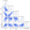 |
Fig. C.3. Same as Fig. C.2], but for V42. |
| In the text | |
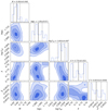 |
Fig. C.4. Same as Fig. C.2], but for V43. |
| In the text | |
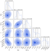 |
Fig. C.5. Same as Fig. C.2], but for V61. |
| In the text | |
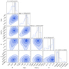 |
Fig. C.6. Same as Fig. C.2], but for V76 |
| In the text | |
Current usage metrics show cumulative count of Article Views (full-text article views including HTML views, PDF and ePub downloads, according to the available data) and Abstracts Views on Vision4Press platform.
Data correspond to usage on the plateform after 2015. The current usage metrics is available 48-96 hours after online publication and is updated daily on week days.
Initial download of the metrics may take a while.