| Issue |
A&A
Volume 702, October 2025
|
|
|---|---|---|
| Article Number | A102 | |
| Number of page(s) | 22 | |
| Section | Extragalactic astronomy | |
| DOI | https://doi.org/10.1051/0004-6361/202453236 | |
| Published online | 13 October 2025 | |
GA-NIFS: The highly overdense system BR1202-0725 at z ∼ 4.7
A double active galactic nucleus with fast outflows plus eight companion galaxies
1
Scuola Normale Superiore, Piazza dei Cavalieri 7, I-56126 Pisa, Italy
2
INAF – Osservatorio Astrofisco di Arcetri, largo E. Fermi 5, 50127 Firenze, Italy
3
Centro de Astrobiología (CAB), CSIC-INTA, Ctra. de Ajalvir km 4, Torrejón de Ardoz, E-28850 Madrid, Spain
4
European Space Agency, c/o STScI, 3700 San Martin Drive, Baltimore, MD 21218, USA
5
University of Oxford, Department of Physics, Denys Wilkinson Building, Keble Road, Oxford OX13RH, United Kingdom
6
Sorbonne Université, CNRS, UMR 7095, Institut d’Astrophysique de Paris, 98 bis bd Arago, 75014 Paris, France
7
Kavli Institute for Cosmology, University of Cambridge, Madingley Road, Cambridge CB3 0HA, UK
8
Cavendish Laboratory - Astrophysics Group, University of Cambridge, 19 JJ Thomson Avenue, Cambridge CB3 0HE, UK
9
Max-Planck-Institut für extraterrestrische Physik (MPE), Gießenbachstraße 1, 85748 Garching, Germany
10
Dipartimento di Fisica e Astronomia, Università di Firenze, Via G. Sansone 1, 50019 Sesto F.no (Firenze), Italy
⋆ Corresponding author: This email address is being protected from spambots. You need JavaScript enabled to view it.
Received:
29
November 2024
Accepted:
1
July 2025
Abstract
Distant quasars (QSOs) in galaxy overdensities are considered key actors in the evolution of the early Universe. In this work, we performed an analysis of the kinematic and physical properties of the BR1202-0725 system at z ∼ 4.7, one of the most overdense fields known in the early Universe, consisting of a QSO, a sub-millimetre galaxy (SMG), and three Lyman-α emitters. We used data from the JWST/NIRSpec integral field unit to analyse the rest-frame optical emission of each source in the system. Based on the continuum and Balmer line emission, we estimated a bolometric luminosity of log(Lbol/[erg s−1]) = 47.2 ± 0.4 and a black hole mass of log(MBH/M⊙) = 10.1 ± 0.5 for the QSO, which are consistent with previous measurements obtained with ground-based observations. The NIRSpec spectra of the SMG revealed, instead, unexpected [O III] and Hα+[N II] profiles. The overall [O III] line profile is blueshifted by more than 700 km s−1relative to the systemic velocity of the galaxy. Additionally, both the [O III] and Hα+[N II] lines show prominent broad (∼1300 km s−1), blueshifted wings associated with outflowing ionized gas. The analysis of NIRSpec and X-ray observations indicates that the SMG likely hosts an accreting supermassive black hole, which is supported by the following results: (i) the excitation diagnostic diagram is consistent with ionization from an active galactic nucleus (AGN); (ii) the X-ray luminosity is higher than 1044 erg s−1; and (iii) it hosts a fast outflow (vout ∼ 5000 km s−1), comparable to the ones observed in luminous QSOs. Therefore, the QSO-SMG pair of BR1202-0725 represents one of the highest-redshift double AGNs found to date, with a projected separation of 24 kpc. Finally, we investigated the environment of this system and found four new galaxies, detected in both [O III] and Hαemission, at the same redshift of the QSO and within a projected distance of 5 kpc from it. This overdense system includes at least ten galaxies in a field of view of only 980 kpc2.
Key words: ISM: jets and outflows / galaxies: high-redshift / quasars: supermassive black holes
© The Authors 2025
 Open Access article, published by EDP Sciences, under the terms of the Creative Commons Attribution License (https://creativecommons.org/licenses/by/4.0), which permits unrestricted use, distribution, and reproduction in any medium, provided the original work is properly cited.
This article is published in open access under the Subscribe to Open model. This email address is being protected from spambots. You need JavaScript enabled to view it. to support open access publication.
1. Introduction
Cosmological numerical simulations expect luminous active galactic nuclei (AGNs) to reside in some of the most overdense regions of the Universe (Ni et al. 2020; Habouzit et al. 2019; Valentini et al. 2021; Weinberger et al. 2018; Costa et al. 2014; Di Matteo et al. 2012; Sijacki et al. 2009; Zana et al. 2022, 2023; Barai et al. 2018). In such fields, both the growth of supermassive black holes (BHs) and the formation of new stars are thought to be triggered by galaxy mergers and interactions.
However, whether distant quasars (QSOs) form and evolve in galaxy overdensities is still an open question (see e.g., Villforth 2023, and references therein). Rest-frame UV observations with ground-based telescopes and the Hubble Space Telescope (HST) have led to contrasting results. Some studies have found a large number of galaxies within a few megaparsecs of z ∼ 6 QSOs (Bosman et al. 2020; Meyer et al. 2022; Overzier 2022; Zheng et al. 2006; Farina et al. 2017; Mignoli et al. 2020), while others have reported no sources or only a few galaxies in the vicinity of the QSO (e.g., Willott et al. 2005; Morselli et al. 2014; Simpson et al. 2014). Even observational programmes conducted with the Atacama Large Millimeter/submillimeter Array (ALMA) have produced differing and sometimes contradictory results in the identification of companion galaxies near high-redshift QSOs. Some studies have identified up to three [C II] emitters in the ∼30″ × 30″ ALMA field of view (FoV; corresponding to a physical scale of ∼180 × 180 kpc2 at z ∼ 6), while others have only reported the emission of the QSOs (Decarli et al. 2017, 2018; Willott et al. 2017; Neeleman et al. 2019; Venemans et al. 2019, 2020; Bischetti et al. 2024). However, Zana et al. (2022, 2023) show that the dust obscuration, angular resolution, and data sensitivity may explain the different results obtained with HST. The small FoV and frequency coverage of ALMA can also explain the scatter in the number of detected satellite galaxies among different observations.
The launch of the James Webb Space Telescope (JWST) has opened a new window on the study of galaxy overdensities at high redshift through rest-frame optical emission lines. NIRCam Wide Field Slitless Spectroscopy (WFSS) observations have revealed more than ten [O III] emitters within a few megaparsecs of the z ∼ 6 QSOs J0305–3150 and J0100+2802 (Wang et al. 2023; Kashino et al. 2023). Only a few of these sources had previously been detected with HST and ALMA. Additionally, NIRSpec observations in integral field spectroscopy (IFS) mode have enabled detailed investigations of the close environment of high-z sources, finding a high prevalence of overdensities (e.g., Jones et al. 2025; Rodríguez Del Pino et al. 2024; Arribas et al. 2024; Lamperti et al. 2024). Many AGNs and QSOs at z > 3 followed up on with NIRSpec IFS show the presence of at least one companion galaxy up to 30 kpc and ±1000 km s−1of the main target (Perna et al. 2025; Marshall et al. 2023, 2024; Loiacono et al. 2024; Übler et al. 2023, 2024). Some of these companions show spectroscopic features associated with AGN ionization, indicating that the system may host a double or even a triple AGN. Analyzing a sample of AGNs at z ∼ 3, Perna et al. (2023) conclude that dual AGNs with projected separations below 30 kpc may be more common (by at least a factor of 2 to 3) than what is predicted by the most recent cosmological simulations (De Rosa et al. 2019; Volonteri et al. 2022). Specifically, the companion galaxies of five out of 16 AGNs (i.e. ∼20–30%) have optical emission line flux ratios consistent with AGN excitation. In comparison, the above theoretical models predict a dual AGN fraction < 1%.
BR1202-0725 (z ∼ 4.7) is one of the most studied overdense fields at high redshift, acting as a laboratory for studying different galaxy types, all evolving in the same environment. The system (see Fig. 1) is composed of a sub-millimetre galaxy (SMG), a QSO with a SMG-QSO projected separation of 24 kpc, and three Lyman-α emitters (LAEs; LAE1, LAE2, and LAE3; Drake et al. 2020; Carniani et al. 2013; Carilli et al. 2013).
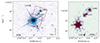 |
Fig. 1. HST ACS F775W filter (i-band; left) and JWST NIRSpec IFU Hα(3.74 μm < λ < 3.75 μm; right) image of BR1202-0725. Dust continuum emission from ALMA in Band 7 is shown as black contours. Star symbols illustrate the position of the three LAEs. North is up, east is to the left. A logarithmic colour scale is used. |
The QSO was observed for the first time by Irwin et al. (1991) and was the first object at z > 4 to be detected in CO emission (Ohta et al. 1996). The optically obscured SMG was also found in these observations, at ∼4″ to the north-west of the QSO (see also Omont et al. 1996; Iono et al. 2006). Both the QSO and the SMG have far-infrared (FIR; ∼40–500 μm) luminosities higher than 1013 L⊙ (Omont et al. 1996; Iono et al. 2006; Carilli et al. 2002), which suggest a very strong star formation activity (SFR > 1000 M⊙ yr−1; Carilli et al. 2013) and which according to the commonly accepted paradigm are likely triggered and sustained by merger events.
The QSO exhibits a large Lyα halo (∼55 kpc, surface brightness > 1 × 10⁻¹⁷ erg s−1 cm−2 arcsec−2; Drake et al. 2020) with high velocity widths (FWHMLyα ∼ 1000 km s−1), probably coupled with the bridge of gas located between the QSO and the SMG observed in [C II] 158 μm (Wagg et al. 2012; Carilli et al. 2013; Carniani et al. 2013). The QSO contains a mass of ∼8 × 10¹⁰ M⊙ of cold molecular gas (derived from the CO(J = 1–0) line luminosity; Riechers et al. 2006). The CO emission of the QSO can be separated into at least two components: the main one (FWHMCO= 700 km s−1), with kinematics compatible with a rotating disc, and another one separated by +0.4″ in declination that has a velocity shift of 180 km s−1and is likely another fainter galaxy in the merger (Salomé et al. 2012). The QSO also shows an excess of emission in the red wing of the line profile of [C II], which suggested an outflow of atomic gas from the QSO expelling mass at a rate of Ṁout ∼ 80 M⊙ yr−1 (Carilli et al. 2013).
The SMG was detected in [C II] line emission with L[C II] = 1010 L⊙ and its ratio, L[C II]/LFIR = (8.3 ± 1.2) × 10−4, is in agreement with previous high-redshift studies. The analysis of the CO(5–4) observations indicates the presence of a companion galaxy at 0.6″ to the west-north-west of the SMG with a relative velocity of +600 km s−1(see Fig. 4 of Salomé et al. 2012).
LAE1 (zLyα = 4.703) is located north-west of the QSO in the direction of the [C II] bridge and LAE2 (zLyα = 4.698) towards the south-west (see left panel of Fig 1), both at the same redshift as the QSO. These objects were spectroscopically confirmed by the detection of Lyα emission in Hu & McMahon (1996) and Williams et al. (2014), respectively. In LAE1, the [N II] 122 μm emission (Decarli et al. 2014; Pavesi et al. 2016; Lee et al. 2019) and the absence of high-ionization emission lines in the UV spectrum obtained with the FORS2 on the VLT (N Vλ1240 Å, Si IVλ1396 Å, C IVλ1549 Å, and He IIλ1640 Å; Williams et al. 2014) suggest that this source is not photoionized by the QSO. Similarly, LAE2 also lacks high-ionization emission lines; this, together with the [C II] 158 μm/[N II] 122 μm ratio for LAE2, indicates that its emission is dominated by H II regions and may be driven by star formation (L[C II]/L[N II] = 2.3 ) and the CO(2-1) observations suggest that it has a considerable reservoir of molecular gas (∼4 × 10¹⁰ M⊙, Jones et al. 2016). These observations led to the conclusion that star formation is the primary source of emission for all the LAEs in the system. An additional companion (LAE3; zLyα = 4.7019) discovered by Drake et al. (2020) and located 5″ north of the QSO, shows an SFR(Lyα) of 5 M⊙ yr−1 and an EW(Lyα) > 34.05 Å, consistent with star formation being the primary driver of Lyα emission.
In this work, we present new JWST NIRSpec IFS observations of BR1202-0725. We analyse the kinematic and physical properties of the main objects presented above, and we also study four newly identified galaxy companions that are part of the system. The observations on which the work is based are presented in Sect. 2 together with an overview of the data reduction. Section 3 provides a detailed description of the system based on these observations and illustrates the data analysis. Sections 4 to 6 focus on the results obtained for QSO, SMG, and LAEs, respectively. In the latter, we also present the four newly detected galaxy companions of the QSO in addition to the LAEs and the ones found by Salomé et al. (2012). The discussion is given in Sect. 7 and a summary of our results and final conclusions are presented in Sect. 8. Throughout this paper, we adopt the standard cosmological parameters H0 = 70 km s−1 Mpc−1, ΩM = 0.30, and ΩΛ = 0.70, giving a cosmology-corrected scale of 6.48 kpc arcsec−1 at z = 4.7.
2. Observations and data reduction
We used JWST NIRSpec IFS (Jakobsen et al. 2022; Böker et al. 2023, 2022) observations obtained as part of the NIRSpec IFS GTO programme ‘Galaxy Assembly with NIRSpec IFS’ (GA-NIFS)1. These data cover the QSO, the SMG, and two LAEs (LAE1 and LAE2) with two different pointings (covering 3.6 × 6.5 arcsec2) that overlap by 10% because the main sources are spatially separated by a projected distance larger than 3 arcsec (see Fig. 1).
The observations were acquired on July 1 2023. Two disperser/filter combinations were used: G235H/G170LP and G395H/F290LP, with a spectral resolution of R ∼ 2700 and covering the wavelength ranges 1.66–3.05 μm and 2.87–5.14 μm, respectively (corresponding to the rest-frame range 2910–9020 Å at a redshift ∼4.7). The selected spectral configuration covers the main rest-frame optical emission lines at the redshift of the system, including the Balmer lines (Hα, Hβ), [O III] λλ4959,5007 Å, [N II] λλ6548,84 Å, and [S II] λλ6717,31 Å. Each grating was observed for 3559 s in two different exposures to target the QSO and the SMG.
We retrieved the raw data from the MAST (Barbara A. Mikulski Archive for Space Telescopes) archive. Then, we reduced them with a customized version of the JWST pipeline (version 1.14.0), using the Calibration Reference Data System (CRDS) context jwst_1225.pmap. Some modifications to the pipeline allowed us to improve the data quality. They are described in detail in Perna et al. (2023), but here we summarize the major changes. First, we applied the ‘calwebb_detector1’ step of the pipeline to account for detector level correction. Before calibrating the count-rate images through the ‘calwebb_spec2’ module of the pipeline, we corrected them by subtracting the 1/f noise through a polynomial fitting. We identified and removed outliers directly in the calibrated 2D images by applying an algorithm similar to ‘lacosmic’ (van Dokkum 2001). Briefly, we computed the derivative along the dispersion direction, and we rejected the 98th percentile of the distribution (see D’Eugenio et al. 2024, for details). The final data cube was created by combining the individual calibrated 2D exposures using the ‘drizzle’ weighting and obtaining a cube with a spaxel size of 0.05″.
We also used [C II] 158 μm and adjacent continuum observations from ALMA in Band 7 to compare the shape of the [C II] spectrum of the SMG with the ones of [O III] and Hαfrom JWST and to compare the location of the dust continuum with that of Hα. We retrieved the raw visibilities of programme 2019.1.01587.S (PI: F. Lelli) from the ALMA archive and calibrated them with the Common Astronomy Software Application (CASA) by using the script included in the dataset. By using the task ‘tclean’, we cleaned the calibrated visibilities using a ‘Briggs’ weighting scale and a robust parameter equal to 0.5 to obtain the final data cube. The data cube has a beam size of 0.17″ × 0.12″, roughly matching the NIRSpec IFS resolution (∼0.09″–0.15″; D’Eugenio et al. 2024).
We used HST observations to calculate the astrometric offsets between the NIRSpec integral field unit (IFU) and the ALMA data (see Sect. 3.1). They were acquired on May 24 2005 with the Advanced Camera for Surveys (ACS) and the F775W filter. These data are part of proposal ID 10417 (PI: X. Fan) and are organized into four exposures and a total exposure time of 9445 s. The data were downloaded from the Hubble Legacy Archive (HLA) and reduced by the Space Telescope Science Institute (STScI) using available calibration files taken for this observation and accounting for the different dithering positions.
Finally, we also employed Chandra archival data to investigate whether the SMG emits X-rays. BR1202-0725 was observed twice with ACIS-S (Advanced CCD Imaging Spectrometer), once during Cycle 3 for 10 ks (ObsID 3025, presented in Iono et al. 2006) and a second time in Cycle 9 for 30 ks (ObsID 9232, presented in Li et al. 2021). The results of the X-ray data analysis are presented in Sect. 7.2.
3. Data analysis
3.1. Astrometry correction
Since astrometric offsets between the NIRSpec IFU data and the position of the sources on the sky have been reported in the literature (e.g., Perna et al. 2023; Jones et al. 2025, 2024), we registered the JWST observations to the HST image (ACS-F775W). We verified the astrometric accuracy of the HST image by comparing the position of the star in the FoV with the coordinates reported in Gaia Data Release 3 catalog (Gaia Collaboration 2023). We used the position of the QSO to register the JWST data to HST one and found a shift of ΔRA = +0.199 arcsec and ΔDec = −0.144 arcsec.
In this work, we assumed that the ALMA astrometry is sufficiently precise for our purpose, considering that the ALMA positional accuracy varies from 5% to 20% of the beam depending on the S/N, which corresponds to an accuracy of 0.03 arcsec for a beam of 0.17″ × 0.12″. The high S/N ensures that the ALMA astrometry is correct within 1 NIRSpec spaxel.
3.2. BR1202-0725
The well-studied BR1202-0725 system has been observed in a wide range of molecular and atomic lines (e.g., Omont et al. 1996; Salomé et al. 2012; Carilli et al. 2013; Benford et al. 1999; Lu et al. 2017). However, this is the first time it was observed in rest-frame optical emission lines. The left panel of Fig. 1 shows the HST ACS image in the F775W filter, covering the spectral range 6801–8630 Å (corresponding to the UV rest frame emission between 1193 Å and 1514 Å at z = 4.7) with the two JWST pointings used in this paper superimposed. The JWST map at the wavelength of the Hα emission line (3.74 μm < λ < 3.75 μm) is shown in the right panel. The ALMA dust continuum emission is shown as black contours.
The QSO is the most prominent source in Hαin the FoV of the NIRSpec IFS data, appearing in the bottom left part of the map, and it is dominated by the point spread function (PSF) emission. However, LAE1 is also very prominent, showing a spatially resolved structure that could be connected to the bridge between the QSO and the SMG observed in [C II] (Carniani et al. 2013). The SMG is located in the top right part of the map, showing an elliptical appearance in the ionized gas. This object has been studied in other FIR and millimetre/sub-millimetre emission lines, such as [N II] at 122 and 205 μm (rest-frame), with ALMA and the IRAM Plateau de Bure Interferometer (PdBI) (Decarli et al. 2014; Drake et al. 2020). Despite some attempts to study the optical emission with SINFONI, that results in a non-detection of the [O II] λλ3726, 29 Å doublet (Couto et al. 2016), and an integrated spectrum from the AKARI space telescope encompassing the Hαemission of the QSO and SMG (Jun et al. 2015), this is the first time that this optically obscured, sub-millimetre-bright object has been able to be spatially resolved at rest-frame optical wavelengths, thanks to the high resolution and sensitivity of JWST.
3.3. Point spread function modelling
One of the main goals of this work is identifying the presence of companion galaxies close to the QSO and studying their properties. Therefore, it is fundamental to remove the point-like emission of the QSO that outshines a large fraction of the IFS FoV.
Following the approach of Decarli et al. (2024), we generated a set of 17 images of the PSF by integrating the emission of the QSO in different wavelength bands with a width varying between 0.01 μm and 0.13 μm depending on the presence of either emission lines or cosmic rays in the field (see Fig. A.1). The selected bands exclude the brightest forbidden emission lines, such as [O III], [S II], and [N II], as well as narrow Balmer lines, because they are not associated with the spatially unresolved emission of the accretion disc, and are therefore likely to be spatially extended.
We interpolated these PSF images at each wavelength of the data cube, and we obtained a data cube with the normalized image of the PSF at each wavelength. Then, we scaled the flux of each one using an aperture of 0.25″ centred on the peak of the QSO (see Decarli et al. 2024). Finally, we subtracted the PSF models from the JWST data. Fig. 2 shows the emission of the QSO at the wavelength of the Hβ emission line (2.75 μm < λ < 2.77 μm, observed frame) before and after subtraction of our modelled PSF. We notice that our procedure slightly over-subtracts the QSO emission at the centre; hence, the flux measurements in this region are not reliable. Therefore, we masked a region of radius of 0.2″ from the centroid of the QSO in the PSF-subtracted data cube and limited our analysis to the emission at greater distances from the bright source.
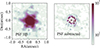 |
Fig. 2. Original (left) and PSF-subtracted (right) maps of the QSO at the wavelength corresponding to the Hβ emission line. |
3.4. Aperture correction
The aperture correction is necessary to determine the total emission flux of the targets, since the PSF of the instrument depends on the wavelength. Following Loiacono et al. (2024), we determined the flux losses from 1.7 μm to 5.2 μm for four different apertures by using the PSF models generated in Sect. 3.3. Figure B.1 reports the fraction of flux recovered from the four apertures with respect to an aperture with a radius of 1 arcsec, which is large enough to recover all the emission of point-like sources. All spectra and fluxes reported hereafter have been corrected for flux losses, depending on the selected aperture and wavelength. We present the procedure and the results in Appendix B.
4. QSO
Figure 3 illustrates the spectrum of the QSO extracted from an aperture of R = 0.5 arcsec and located at the peak of the emission (RA = 181.34634 deg, Dec = −7.70906 deg). We calculated the errors on the integrated spectrum from the error extension of the data cube in the same spaxels of the selected region propagating them in quadrature (see Appendix C). The spectrum clearly reveals broad emission lines of Hαand Hβ, and Fe II emission lines arising from the broad line region (BLR).
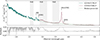 |
Fig. 3. JWST/NIRSpec rest-frame optical spectrum of the QSO in the two gratings/filters G235H/F170LP and G395H/F290LP (green and purple lines, respectively), extracted from an aperture of R = 0.5″. The brightest nebular lines are marked and the Fe II multiplet bands are highlighted in grey. The dashed green line shows the broken power-law continuum model fitted to reproduce the featureless continuum emission. The grey line in the bottom panel shows the residuals of the fitting. |
We initially modelled the featureless continuum emission of the QSO. A simple power-law function is usually adopted to reproduce the multi-blackbody emission of the accretion disc (e.g., Loiacono et al. 2024), but given the extended wavelength range covered by the NIRSpec data, we adopted two power-law functions as follows:
 (1)
(1)
where A is the normalization, λ0 the break wavelength, and α1 and α2 the power-law indexes. This profile has been widely used to reproduce the continuum emission of local QSOs (Vanden Berk et al. 2001), which change slope at the rest-frame wavelength of ∼5000 Å due to the contribution of the host galaxy.
We fitted the line-free spectral regions of the spectrum with the function in Eq. (1), constraining the break wavelength values in the following range: 2.5 μm < λ0obs < 5 μm. Figure 3 shows the QSO spectrum together with the continuum model, while the fitted parameters are shown in Table 1. Considering a redshift of z = 4.6943 (Carniani et al. 2013), we found a rest-frame value for the break wavelength of 5107 ± 108 Å, comparable to others found in the literature for QSOs at a similar redshift (e.g., Loiacono et al. 2024).
Fitted continuum parameters for the QSO.
Typical type 1 QSO spectra such as the one reported show the presence of a forest of Fe II emission bumps. The analysis of the Fe II multiplets is not among the aims of this paper. However, it is important to obtain a continuum- and Fe II-free spectrum in order to fit the optical emission lines to derive QSO properties such as the BH mass. In particular, appropriately modelling the prominent Fe II multiplets in the rest-frame wavelength region between 4700 and 5400 Å is critical, since they are blended with Hβ and [O III] λλ4959,5007 Å emission lines.
We tried to reproduce the Fe II emission with the following three different templates: Tsuzuki et al. (2006, T+06), Véron-Cetty et al. (2004, VC+04), and Boroson & Green (1992, BG+92). The results are shown in Fig. 4. None of them was able to accurately reproduce all the Fe II emission features in the spectrum. However, we discarded the results obtained with Tsuzuki et al. (2006) and Boroson & Green (1992) templates because they overpredict the flux emission at the wavelength range of the [O III] (see Park et al. 2022). We have thus assumed as a fiducial model the results obtained with the Véron-Cetty et al. (2004) Fe II template.
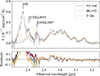 |
Fig. 4. QSO rest-frame optical continuum-subtracted spectrum (grey line) in the spectral region 4700–5400 Å. The emission lines Hβ and [O III] λλ4959,5007 Å (marked with vertical lines) are blended with the Fe II emission, which can be clearly seen at ∼3 μm. The following fitted Fe II templates are shown: Véron-Cetty et al. (2004, VC+04, red line), Boroson & Green (1992, BG+92, blue line), and Tsuzuki et al. (2006, T+06, yellow line). The lines in the bottom panel show the different residuals of the fitting. |
Finally, we fitted the brightest nebular lines present in the integrated continuum-subtracted spectrum, Hβ, [O III] λλ 4959,5007 Å, [N II] λλ6548,84 Å, Hα, and [S II] λλ6717,31 Å, using a combination of Gaussian profiles convolved with the line spread function of the instrument. We have used two Gaussian components: (i) a ‘Narrow’ component with σ < 600 km s−1, and (ii) a broad one (dubbed ‘Outflow’) with 400 km s−1< σ < 2000 km s−1. For the Balmer recombination lines, Hα and Hβ, we added an additional Gaussian component with a velocity dispersion spanning a range of 1000 km s−1 < σ < 5000 km s−1to reproduce the emission from the BLR. We tied the kinematics of each Gaussian component for each emitting species (centroid and line width). The two emission lines of the [O III] and [N II] doublets originate from the same upper level, then we fixed the intensity ratios between each line of these doublets to their theoretical values: I([N II] λ6584)/I([N II] λ6548) = 2.94 and I([O III] λ5007)/I([O III] λ4959) = 3 (Osterbrock & Ferland 2006). We also fixed the Hα/Hβratio of the Narrow and Outflow components to take values of 2.3 < Hα/Hβ< 10. We included the Véron-Cetty et al. (2004) Fe II template in the fitting, by allowing its amplitude and velocity dispersion to vary.
In Table 2, we report the emission line velocities and velocity dispersions for each component and the emission-line intensities of the nebular lines after the aperture correction (see Sect. 3.4). Figure 5 shows the fitted profiles for each component. We can see that the multi-component fitting accurately reproduces the spectrum at the wavelengths of the emission lines, with a narrow and a broad component with velocity dispersions of 660 ± 30 km s−1and 1360 ± 80 km s−1, respectively. The BLR is blueshifted by −410 km s−1relative to z = 4.6943 (Carniani et al. 2013) and has σ = 4160 ± 60 km s−1.
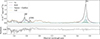 |
Fig. 5. Continuum-subtracted JWST NIRSpec spectrum of the QSO. The best-fit model is shown with a solid black line, while the results of the individual components are reported with different colours: the dashed blue line shows the Narrow + Outflow components, and the dotted purple line corresponds to the BLR component. The fitted Véron-Cetty et al. (2004) Fe II template (VC+04) is shown with the dash-dotted orange line. |
We stress that the Narrow and Outflow components in the fitting are strongly affected by degeneracies, and the Fe II multiplets present in the spectrum also influence the values obtained for the [O III] emission line. Therefore, these results should be interpreted with caution. For the BLR component, the velocity dispersion and amplitude vary depending on the fitting priors. Specifically, the velocity dispersion ranges from 3400 km s−1to 4600 km s−1(mean value of 3900 km s−1with a standard deviation of 400 km s−1), which translates into an Hαemission line flux range of 470–660 ×10−17 erg s−1 cm−2. However, as is shown in Sect. 7.3, the different BH masses obtained from the above range of values are well within the uncertainty on the calibration used to estimate them, and therefore they are consistent with each other.
5. SMG
Figure 6 shows the integrated spectrum of the SMG located ∼24 kpc north-west of the QSO (see Fig. 1). The spectrum was extracted from an aperture of R = 0.3 arcsec centred on the position RA = 181.34575 deg and Dec = −7.70825 deg. In contrast to the QSO, the continuum emission from the SMG is detected with low S/N and its intensity does not depend strongly on the wavelength.
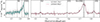 |
Fig. 6. JWST NIRSpec rest-frame optical spectrum of the SMG in the two gratings/filters G235H/F170LP and G395H/F290LP (blue and red lines, respectively), extracted from an aperture of R = 0.3″. The errors of the spectrum are shown in light grey. |
The G395H data clearly reveal blended Hα and [N II] emission and the [S II] doublet. He Iλ5875 Å and [O I] λ6300 Å are also visible in the spectrum, with lower signal-to-noise ratios (S/N = 2.6). At lower wavelengths, the [O III] λ5007 Å is detected with a S/N higher than 21, while the Hβ line is not detected due to the high dust attenuation of the galaxy.
We note that the peak of [O III] is blueshifted with respect to the other optical lines observed in the NIRSpec data. By adopting the systemic redshift of z = 4.6891 determined from [C II] and CO FIR emission lines (see Carniani et al. 2013 and Salomé et al. 2012, respectively), we find that the peak of Hα+[N II] is consistent with the systemic redshift of the galaxy, while the peak of the [O III] line is shifted by −1000 km s−1(Fig. 7). The profiles of both the [O III] doublet and Hα+[N II] are very broad and show an asymmetric shape with a prominent emission at shorter wavelengths that suggests the presence of galactic outflows (e.g., Cresci et al. 2015; Carniani et al. 2015; Harrison et al. 2015, 2016; Balmaverde et al. 2016; Brusa et al. 2016; Perna et al. 2017; Leung et al. 2019; Vayner et al. 2021, 2024; Venturi et al. 2023; Speranza et al. 2024).
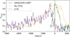 |
Fig. 7. Comparison of the SMG line profiles of the [O III], Hα+[N II], and [C II] emission lines in velocity space. All line profiles are normalized to their peak value. The vertical dotted black line indicates the zero velocity at the systemic redshift of z = 4.6891 for [O III] λ5007, Hα, and [C II] emission lines. |
We fitted the brightest nebular lines of the SMG by using a combination of Gaussian profiles. Due to the complexity of the blended Hαand [N II] profiles (see Fig. 6), we started by fitting only the [O III] doublet emission to determine the kinematics of the blueshifted broad wings. We used a combination of two Gaussian components: (i) a narrow component with σ < 400 km s−1, and (ii) a broad component with 400 km s−1 < σ < 1500 km s−1. We dubbed the narrow and broad components ‘Narrow 2’ and ‘Outflow’. We adopted the label Narrow 2 because this component is not at the systemic redshift of the galaxy defined from [C II] and CO. We used a second-order polynomial to model the continuum in this spectrum.
The upper panel of Fig. 8 shows the best-fit model for the [O III] doublet. The Outflow component has a velocity dispersion of 1300 ± 500 km s−1and is blueshifted by −2450 ± 40 km s−1relative to the systemic velocity of the galaxy. The profile of this line is similar to the broad blueshifted wings observed in luminous QSOs, associated with fast outflowing gas.
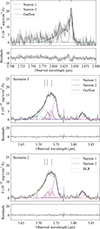 |
Fig. 8. Fitting results for the SMG spectrum, showing the Narrow 1, Narrow 2, BLR, and Outflow components (dotted purple, dashed red, dashed yellow, and dash-dotted blue lines, respectively). The errors considered in the fitting procedure are displayed in grey and the residuals of the fits are shown at the bottom of each panel. Top panel: Fit of the [O III] λλ4959,5007 Å emission lines. The vertical dotted lines mark the position of [O III] at the systemic redshift determined from [C II]. Middle and bottom panels: Fits of the Hα, [N II] λλ6548,6584 Å, and [S II] λλ6717,6731 Å emission lines for the first (outflow) and second (BLR) scenarios described in Sect. 5. The vertical black lines indicate the position of the emission lines for the Narrow 2 component found in [O III]. |
The Narrow 2 instead has a velocity dispersion consistent with what is expected from a rotating massive galaxy (σ = 300 ± 100 km s−1), but is blueshifted by −760 ± 90 km s−1relative to the systemic redshift determined from [C II]. This remarkable velocity shift suggests that this emission is associated with outflowing gas. A similar shift has been observed in AGNs called ‘blue outliers’, in which the peak of the [O III] is blueshifted by more than −250 km s−1with respect to the peak of Hαand Hβlines (Zamanov et al. 2002). In the local and z ∼ 1 Universe, these features are observed in highly accreting AGNs, and the velocity shift is thought to be due to strong nuclear outflows (Zamanov et al. 2002; Marziani et al. 2003; Lanzuisi et al. 2015; Marziani et al. 2016; Cracco et al. 2016; Perna et al. 2021, 2023). In conclusion, as similar profiles have been observed in other AGNs, we believe that the entire [O III] emission line of the SMG (Narrow 2+Outflow) is tracing a ionized outflow.
We stress that the extraction aperture of the spectrum (radius = 0.3″) encloses all the outflow emission. It does not encompass the whole galaxy emission, which is more extended than the aperture, but this does not affect our analysis, which focuses on the properties of the broad component rather than on those of the extended galaxy emission.
As was discussed above, the blended Hα+[N II] profile is complex, and the results strongly depend on the number of components used to reproduce the shape of the emission lines. Therefore, we considered the two following possible scenarios: (1) the broad asymmetric profile of the complex line is due to the presence of galactic outflows; (2) the SMG hosts a type 1 AGN and the very broad component is associated with the emission of the BLR. We discuss these alternative scenarios in the following. Both are practically identical when taking into account the statistical confidence of the best-fit models. Also, a combination of both is possible; therefore, we discuss the two extreme scenarios in the following sections.
5.1. Scenario 1: High-velocity outflow hosted by the SMG
The two components (Outflow and Narrow 2) adopted to model the [O III] line profile, significantly blueshifted relative to the systemic velocity, are not sufficient to reproduce the profile of the Hα, [N II], and [S II]. Therefore, for the five emission lines of these three species we added an additional Gaussian component with σ < 500 km s−1dubbed Narrow 1. We also fixed the kinematics (centroid and line width) of the Narrow 2 and Outflow components to the best-fit results from the [O III] fitting process.
The middle panel of Fig. 8 illustrates the best-fit model (Reduced chi-squared, χ = 13.89) and Table 3 reports the best-fit values for the free parameters. The Hα+[N II] complex is reproduced well with this fitting and the Narrow 1 centroid is within 110 km s−1of the systemic redshift of the galaxy. As the line spread function of the instrument has a full width at half maximum (FWHM) of ∼100 km s−1, we can conclude that Narrow 1 arises from the gas at rest in the galaxy. This component is also consistent with the kinematics of the He Iλ5875 Å and [O I] λ6300 Å nebular emission lines, and also with that of [C II] and CO lines. The kinematics of this component is consistent with being gas in the host, but the velocity dispersion (σ ∼ 470 km s−1) is larger than that of [C II] and CO lines (σ[C II] ∼ 307 km s−1and σCO ∼ 313 km s−1), which may be due to turbulent and disturbed ionized gas at large scales due to interactions with the other members of the group (see Salomé et al. 2012; Lehnert et al. 2020).
Remarkably, no Hα Outflow component is found in this fitting, with only [N II] doublet lines being non-zero. However, there could be some degeneracies in the fitting due to the complexity and broadening of the blended Hα+[N II] profile. The best-fit model indicates that [N II]-to-Hαflux ratio of the Outflow component is higher than 7 (log([N II] λ6584 Å/Hα) > 0.85), an extreme line ratio that suggests that the blueshifted Hα component is blended with the [N II] due to the degeneracy.
We determined the lower limit on the reddening by calculating the standard deviation of the spectrum at the position of the Hβ emission line, obtaining a value of 0.85 × 10⁻²⁰ erg s−1 cm−2 (1σ). By assuming that the Balmer lines have the same line width as the other nebular lines, we found that the Balmer ratios for the narrow components are HαNarrow 1/HβNarrow 1 > 9.2 and HαNarrow 2/HβNarrow 2 > 7.1. The extinction, AV, can be calculated by adopting the Galactic extinction law of Miller & Mathews (1972), with a specific attenuation of RV = 2.97 and the theoretical ratio Hα/Hβ = 2.863 from Osterbrock & Ferland (2006, for ne = 100 cm−3, Te = 104 K, case B recombination). We thus obtained AV, Narrow 1 > 3.5 mag and AV, Narrow 2 > 2.7 mag.
5.2. Scenario 2: The SMG as a Type 1 AGN
We now present the other more ‘extreme’ scenario in which the broad blueshifted Hα component might be associated with the emission of a BLR. To test the case in which the broad component in Hα+[N II] is due to emission from the BLR, we replaced the Outflow component in fitting this line complex with another Gaussian profile dubbed BLR that is only associated with the Hα line, allowing its velocity dispersion to vary between 1000 and 5000 km s−1, as is typical of BLRs in AGNs. The results of the spectral fitting are listed in Table 3. We stress that, even if the broad component in Hα+[N II] is due to a BLR and not an outflow, this does not change the fact that the very broad component observed in [O III] (see Sect. 5) can only be explained by the presence of a fast outflow.
The best-fit model (χ = 13.80) illustrated in the bottom panel of Fig. 8 shows that an individual BLR Gaussian profile in Hαwith a velocity dispersion of 1370 km s−1(Table 3) is sufficient to reproduce the prominent wings in the spectrum of Hα+[N II]. However, we note that the component is blueshifted by −1600 km s−1with respect to the systemic velocity of the galaxy. Velocity shifts of BLR lines of thousands of km s−1have already been observed in other AGNs from the Sloan Digital Sky Survey (e.g., Shields et al. 2009; Steinhardt et al. 2012; Eracleous et al. 2012; Li et al. 2022; Zhang 2024; Halpern et al. 1996; Runnoe et al. 2025) and several explanations have been proposed to explain the spectral displacement of the BLR Balmer lines (see Ju et al. 2013; Komossa & Merritt 2008; Gaskell 2010): (a) dense gas clouds forming the BLR are moving on elliptical Keplerian orbits; (b) a recoiling supermassive BH; (c) binary BHs; (d) a perturbed accretion disc. Multi-epoch spectra are necessary to investigate the origin of the blueshifted BLR among the aforementioned explanations; therefore, we refrain from further speculation.
6. LAEs and companions
As BR1202-0725 is one of the most overdense fields known in the early Universe, we exploited the NIRSpec IFS data to study the properties of its environment. The two LAEs, LAE1 and LAE2, are detected with a high level of significance in both spectral configurations of the NIRSpec data in the integrated spectra extracted from apertures of R = 0.6 arcsec and 0.3 arcsec for the two sources, respectively (see Fig. 9).
 |
Fig. 9. JWST NIRSpec rest-frame optical spectra of LAE1 and LAE2 in the two gratings/filters used (G235H/F170LP and G395H/F290LP, blue and red lines, respectively), extracted from apertures of R = 0.6″ and 0.3″, respectively. The errors in the spectra are shown in light grey and the kinematic components used to model the emission lines in LAE1 are marked with different curve styles and colours (the two main narrow components are shown with a dashed black and a dotted purple line, respectively, while the broad component is marked shown with a dashed grey line). The spikes that appear in the Hβ emission line of LAE1 are instrumental artefacts; therefore, the measurements of this emission line in LAE1 are not completely reliable. |
The optical lines of LAE1 reveal a double-horned profile that might suggest the presence of a rotating disc. However, the analysis of the channel maps indicates a scenario of two independent galaxies that partially overlap along the line of sight. Taking into account the relative positions and velocities of these two galaxies, they could be an ongoing merging system (Fig. D.1). The two sources, hereafter dubbed LAE1a and LAE1b, are separated by a projected distance of about ∼2.8 kpc, which is larger than the typical galaxy size at similar redshift and mass (e.g., 1.5–2 kpc; Ormerod et al. 2024). The relative velocity between LAE1a and LAE1b is ≃590 km s−1and their emission lines have similar velocity dispersions of 160 km s−1and 167 km s−1, respectively. Modelling the spectral shape of the line requires an additional broad component (σ = 570 ± 20 km s−1), which may originate from tidal interactions oroutflows.
The other known companion galaxy in the system, LAE2, is detected only in Hα and [S II], whose redshift is consistent, within the errors, with the ones determined from Lyα and [C II]. The Hαemission map features a south-north elongation, but unfortunately the sensitivity of current observations is notsufficient for a spatially resolved kinematic analysis of the Hαemission of the galaxy.
In addition to LAE1 and LAE2, we robustly identified four other companion galaxies (C1, C2, C3, and C4) within 1″ of the QSO by performing a blind line search in the PSF-subtracted data cube. The two panels of Fig. 10 show the emission maps obtained by integrating the PSF-subtracted data-cube over two wavelength ranges including [O III] λ5007 Å line emission at different spectral shifts, 2.86–2.865 μm and 2.85–2.86 μm, respectively. The two wavelength ranges correspond to the spans of velocity 1080–1600 km s−1and 30–1080 km s−1 with respect to the [O III] wavelength redshifted to z = 4.6943. One of the companions (C1) is very bright in [O III] and is located at around 3.25 kpc to the east of the QSO with an apparent elongation to the north-west, while the two other bright sources (C2 and C3) are within a radius of ∼2.3 kpc from the QSO. The last one (C4) is located to the south-west of the QSO. All the sources are detected in both [O III] and Hαand have redshifts within 1200 km s−1from the systemic velocity of the QSO. We extracted the integrated spectra of the new companion galaxies, C1, C2, C3, and C4, from the apertures shown in Fig. 10 (with radii of 0.2, 0.1, 0.15, and 0.1 arcsec for C1, C2, C3, and C4, respectively) and we report them in Fig. 11. A single Gaussian component per line was sufficient to fit the emission lines. The emission line observed fluxes and the main emission line ratios of these newly found sources are reported in the upper part of Table 5, together with those of the LAEs. We stress that the errors on the Gaussian parameters might be larger due to the uncertainties introduced by the PSF subtraction. LAE3 falls outside the FoV of the NIRSpec IFS observations (Fig. 1, left); therefore, we cannot constrain its emission-line properties.
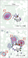 |
Fig. 10. JWST NIRSpec PSF-subtracted maps integrated over the two wavelength ranges reported in each panel, both encompassing [O III] λ5007 Å emission in the same FoV. The QSO position is marked with a plus symbol. The companions found near the QSO are highlighted with red circles, which represent the apertures used to extract their integrated spectra (reported in Fig. 11). |
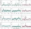 |
Fig. 11. JWST NIRSpec rest-frame optical spectra of the four detected companions, C1, C2, C3, and C4, extracted from apertures of R = 0.2″, 0.1″, 0.15″, and 0.1″, respectively. The errors on the spectrum are shown in light grey. The fitting results are shown with a dashed black line. |
In conclusion, the BR1202-0725 system includes at least ten galaxies, namely the QSO, the SMG, and the companions LAE1a, LAE1b, LAE2, LAE3, C1, C2, C3, and C4, in a projected area of 980 kpc2 (∼0.123 Mpc3, co-moving volume) and within a relative velocity range of ∼1200 km s−1. A similarly large number of companions has also recently been found in SPT0311-58 at z ∼ 6.9 thanks to NIRSpec IFU observations (Arribas et al. 2024). Interestingly, this system shares several similar structural and kinematic properties with BR1202-0725. In particular, it is also formed by two main (dusty) galaxies and about ten nearby companions with relative radial velocities and projected distances similar to what we found in BR1202-0725. Table 4 shows the coordinates, redshifts, velocity shifts, and projected distances of all the galaxies found in this field. All the spectra of the companions show Hα, Hβ, [O III] λλ4959,5007 Å, and [O II] λλ3727,29 Å emission lines, except for LAE2 in which only Hαand [S II] are detected, while LAE1 and C1 also show [Ne III] λ3869 Å (see Figs. 9 and 11). The emission line fluxes and commonly used line ratios are reported in Table 5. The blind line search analysis also revealed the presence of four other candidate emitting sources in the NIRSpec FoV (see Fig. E.1), but the significance of the detection is too low to confirm the origin of the signals and to determine their redshifts. The spectra and coordinates of these candidate sources are reported in Fig. E.2 and Table E.1, respectively.
Coordinates, redshifts, projected distances from the QSO, velocities, and velocity dispersions of the companion galaxies around the QSO of BR1202-0725.
7. Discussion
7.1. Ionization nature of the sources in BR1202-0725
To investigate the ionization mechanism of the various sources in the BR1202-0725 system, we made use of the so-called BPT diagnostic diagram (Baldwin et al. 1981), which exploits the [O III] λ5007 Å/Hβand [N II] λ6584 Å/Hα line ratios to distinguish between star-forming regions and those dominated by AGN radiation, shocks, or non-thermal activity. We report the BPT diagram for the galaxies analysed in this paper in Fig. 12.
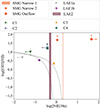 |
Fig. 12. [O III]/Hβ vs [N II]/Hα BPT diagnostic diagram for all objects analysed. The demarcations between H II and AGN-ionized regions (Kauffmann et al. 2003; Kewley et al. 2001, dash-dotted and dashed black lines, respectively) are reported. The vertical lines indicate the [N II]/Hαratio for the two sources for which we do not have values of [O III] and Hβemission lines, with the errors shown by shaded bands (the errors are not visible for the SMG Narrow 1 component). |
For the component associated with the gas at rest in the SMG (SMG Narrow 1, vertical orange line), there is no detection of the [O III] λ5007 Å or Hβ emission lines (see Fig. 8), but both best-fit results of Scenario 1 and Scenario 2 return a log([N II]/Hα) ratio of 0.32 (Table 3), not consistent with star formation processes. The two other components of the SMG (SMG Narrow 2 and SMG Outflow in Scenario 1) have extreme [O III]/Hβand [N II]/Hα, fully consistent with the gas being AGN-photoionized, rather than SF-ionized. Then, the location of the SMG in the BPT together with both scenarios proposed to reproduce the observed integrated spectrum (a BLR or just an outflow with velocity shift of ∼–2500 km s−1), indicate that the SMG hosts an accreting supermassive BH. This supports a dual AGN scenario in this complex system at z ∼ 4.7.
The LAE1a and LAE1b and the companion C1 exhibit [N II]/Hα ratios consistent with star formation processes if they were in the local Universe. However, at high z the traditional low-z BPT becomes insensitive to the mechanism of ionization in this part of the diagram, where both low-metallicity star-forming galaxies and AGN accumulate (see e.g., Feltre et al. 2016; Übler et al. 2023; Maiolino et al. 2024; Hirschmann et al. 2023; Cameron et al. 2023; Scholtz et al. 2025). Therefore, the nature of LAE1a, LAE1b, and C1 is uncertain. For LAE2 there is no detection of either [O III] λ5007 Å or Hβ emission lines; therefore, it might be ionized by either AGN or star formation processes. The nature of the C3 companion is also uncertain because it lies close to the demarcation line between AGN- and star formation-dominated ionization in the BPT diagram. Finally, C2 and C4 are the companions that are mostly consistent with being ionized by the QSO photons.
We calculated the ionization parameter (U) for the companion galaxies in the system using the [O II] λλ3727,29 Å/[O III] λ5007 Å ratio (Díaz & Pérez-Montero 2000). We obtained values ranging from −3.16 to −2.56 on a logarithmic scale (see Table 5).
Assuming that the ionization of the companions is due to star formation and not AGN photons (though this cannot be unambiguously assessed based on the BPT diagram; see Fig. 12), we estimated their metallicities by using the following strong-line diagnostics: R2 = [O II]λλ 3727,29Å/Hβ, R3 = [O III]λ 5007Å/Hβ, O3O2 = [O III]λ5007Å/[O II]λλ3727,29 Å,  = 0.42 R2 + 0.88 R3, N2 = [N II]λ6584Å/Hα, O3N2 = (O III]λ5007 Å/Hβ)/([N II] λ6584 Å/Hα). We adopted the recently introduced diagnostic ratio,
  (Laseter et al. 2024), in place of the traditional R23 = ([O II]λλ3727,29 Å + [O III]λλ4958,5007 Å)/Hβ, since the former is more suited for high-z galaxies. For C1, the only source for which we found a non-zero extinction from Hα/Hβ(AV = 0.16 ± 0.08), we corrected the line fluxes for extinction, assuming a Calzetti et al. (2000) reddening curve with RV = 4.05. To obtain the gas metallicity from the above ratios, we adopted the best-fit polynomial calibrations from Curti et al. (2017, 2020), slightly revisited in Curti et al. (2023, 2024) to better probe the low-O/H regime at high z. Assuming a solar photospheric value 12+log(O/H)⊙ = 8.69 (Asplund et al. 2009), most of the sources have values consistent with Z/Z⊙ ∼ 0.5, while LAE1a and C1 have lower values of ∼0.3 solar, and only C3 has a higher value with Z/Z⊙ = 0.8 (see Table 5).
Emission line observed fluxes (in units of 10−17 erg s−1 cm−2), emission line ratios, and main properties (ionization parameter U, and gas phase metallicity, in terms of oxygen abundance and relative to solar) of the LAEs and confirmed companions, from their integrated spectra reported in Figs. 9 and 11.
Still under the assumption that gas excitation driving line emission is due to star formation and not to the QSO, we find that each of the companions has a star formation rate (SFR) higher than ∼1 M⊙ yr−1 (using the Hα-to-SFR relation from Kennicutt & Evans 2012). We stress again, however, that these estimates should be taken with great caution, given that a contribution to the gas ionization from the bright QSO may affect the line emission fluxes and their ratios. This is especially the case for C2 and C4, whose line ratios are more clearly in the AGN region of the BPT (Fig. 12).
7.2. X-ray detection of the SMG
To further probe the AGN nature of the SMG, we investigated its X-ray properties with archival data from Chandra, the only X-ray facility that can spatially resolve the QSO and the SMG of the system. The X-ray emission of the QSO is detected in both observations, while only Iono et al. (2006) addressed the X-ray emission of the SMG, presenting a tentative detection (below the 3σ level).
We reduced both archival observations (see Sect. 2) with the chandra_repro tool of CIAO v.4.16 (Fruscione et al. 2006) and merged the two datasets with the merge_obs script of CIAO, to maximize the chances of detecting the X-ray emission from the SMG. A soft-band (0.5–2 keV) image (smoothed with a 2-pixel Gaussian kernel) from the resulting data is shown in Fig. 13. With a standard circular extraction region of 1″ radius, we measured three counts at the position of the SMG in the soft band (0.5–2 keV observed-frame) and no counts in the hard band (2–7 keV observed-frame), which is not surprising given the drop of Chandra’s effective area above 2 keV. With a background level of 0.08 counts, we measured 2.9 ± 1.7 net counts in the soft band associated with the SMG, corresponding to the ≃2.8–11.4 keV rest-frame energy range. As a comparison, we detected 33.9 ± 5.8 net counts in the same energy band in a circular aperture of 1″ radius centred on the QSO. We followed the approach of Vito et al. (2019) in testing the significance of the measured X-ray emission at the position of the SMG (i.e. three total counts in the soft band). First, we estimated the probability of this being a spurious detection – that is, due to background fluctuations – applying Eq. (A21) of Weisskopf et al. (2007). We found a false-detection probability of P = 8.9 × 10⁻⁵, making this a detection at ≳4σ. To double-check this result, we measured the probability of detecting three total counts in the soft band by chance by performing aperture photometry in regions of 1″ radius randomly distributed in the field over 106 positions. Considering the full merged field, only 24 regions out of the 106 considered present more than three total counts with a false-detection probability of P = 7.4 × 10⁻⁵. This result could be due to the variation in exposure time from the central region, where the two observations overlap, to the outskirts of each separate field, combined with a larger Chandra PSF moving off-axis. We thus repeated the exercise, restricting the sampled area to the part of the field that was exposed in both observations, finding a false-detection probability of P = 1.5 × 10⁻⁴, and thus a significance of the X-ray emission at the position of the SMG that is slightly less than 4σ.
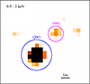 |
Fig. 13. Soft-band (0.5–2 keV) Chandra image of BR1202-0725 (10″ × 10″ box). Data were smoothed with a Gaussian kernel of 2-pixel radius. Circular regions mark the positions of the QSO (blue) and of the SMG (magenta). |
Given this tentative 4σ detection, we measured the X-ray flux of the SMG in the soft band and estimated its intrinsic X-ray luminosity. Assuming a photon index of Γ = 1.9 (in agreement with typical values at these redshifts; e.g., Vignali et al. 2005; Just et al. 2007) and converting the measured count rate with the PIMMS tool v.4.12d2, we found a soft-band observed flux of  . Assuming the same photon index, we converted this flux to intrinsic 2–10 keV luminosity in the two extreme cases of no absorption (NH < 1020 cm−2) and Compton-thick (NH = 1024 cm−2) column densities, which return
  , respectively. The estimated X-ray luminosity is higher than 2 × 1044 erg s−1 at any absorption level and, as such, cannot be explained by SF processes only: previous works estimate a SFR in the range of 1000–5000 M⊙ yr−1 (see Carniani et al. 2013), which corresponds to an X-ray luminosity of 3 × 1043 erg s−1 in the 0.5–8 keV rest-frame band, based on the relation of Mineo et al. (2014). This is less than half the 0.5–8 keV lower limit we get from the estimated X-ray luminosity (
 , assuming no absorption). This tentative X-ray detection thus supports the scenario of the SMG harbouring an AGN.
7.3. Black hole properties
We determined the properties of the BH of the QSO and the SMG from the best-fit results of the spectral fitting. We report them in Table 6. For the SMG, we used the results from Scenario 2, in which we assumed that the broad component of the Hαemission line is associated with the BLR.
Initially, we estimated the impact of dust attenuation on the observed flux of the optical lines by measuring the Balmer decrement. We measured a (Hα/Hβ)BLR ratio of 2.36 (± 0.14) for the BLR component of the QSO. The theoretical ratio in low-density gas is 2.87, assuming Case-B recombination and an electron temperature of Te ∼ 104 K (Osterbrock & Ferland 2006), while it spans a range between 3 and 10 in the dense BLR gas where the optical line depths and collisional effects are different from those in H II regions (Dong et al. 2008; Baron et al. 2016). The ratio measured in the QSO therefore suggests that a dust extinction correction is not necessary.
We used the Hα luminosity to determine the bolometric luminosity of the AGN hosted in the SMG by using the relation from Stern & Laor (2012). This gives a log(Lbol, Hα/[erg s−1]) = 47.2 ± 0.4 for the QSO, which is consistent with the bolometric luminosity calculated from the monochromatic continuum in UV at λ1350 Å, of 47.32 ± 0.02 (Jun et al. 2015) and 47.929 ± 0.029 (Yu et al. 2021). We also determined the bolometric luminosity from the monochromatic luminosity at the rest-frame wavelength of 5100 Å (λL5100) following Netzer (2019):
 (2)
(2)
We infer log(Lbol, 5100/[erg s−1]) = 47.52 ± 0.02, in agreement with the other measurements (see González Lobos et al. 2023).
The properties of the Hα emission line can also be used to estimate the BH mass (MBH), assuming that the gas in the BLR is virialized. In the local Universe, Reines et al. (2013) infer
 (3)
(3)
where LHα and FWHMHα are the line luminosity and width, respectively, of the Hαemission line associated with the BLR (see also Greene & Ho 2005). The calibration has an intrinsic scatter of 0.5 dex (Reines et al. 2013). We thus measured a BH mass of the QSO of log(MBH/M⊙) = 10.1 ± 0.5, which is consistent within 2σ with the estimates derived from Mg II (log(MBH/M⊙) = 9.1 ± 0.3; Carniani et al. 2013) and C IV corrected from outflows effect (log(MBH/M⊙) = 9.65 ± 0.01; Yu et al. 2021). It is important to emphasize that degeneracies in the fitting of the QSO spectrum (see Sect. 4) do not affect the estimated BH mass, since all the values obtained from the different fittings are consistent with each other within the uncertainties, which are dominated by the error on the calibration.
The excitation diagnostic diagrams and the tentative X-ray detection indicate that the SMG hosts an AGN at its centre. We thus estimated its BH mass and bolometric luminosity from the best-fit results of the BLR Hαcomponent inferred in Scenario 2. We measured a lower limit on the Balmer decrement of (Hα/Hβ)BLR > 6, which is within the range of values measured in low-redshift Seyferts and QSOs (Dong et al. 2008; Baron et al. 2016). However, the rest-frame UV emission is heavily obscured due to the high dust content in the interstellar medium, so the measured Hαluminosity (Table 6) is a lower limit. Therefore, the quantities derived for the BH of the SMG are lower limits as well. We thus inferred log(Lbol, Hα/[erg s−1]) > 44.9 and log(MBH/M⊙) > 8.0.
BH properties of the QSO and SMG.
If the mass of the BH of the SMG is confirmed by future observations, BR1202-0725 would be one of the most distant systems with two BHs with similar masses (MBH ≳ 108 M⊙) within a projected distance of 24 kpc (see also Matsuoka et al. 2024; Übler et al. 2024). Simulations of z ∼ 6 luminous QSOs predict that highly accreting supermassive BHs live in overdense fields hosting galaxies with similar stellar and BH masses (Barai et al. 2018; Valentini et al. 2020; Zana et al. 2022; Di Mascia et al. 2021). For example, Di Mascia et al. (2021) show a simulated system similar to the BR1202-0725 one where a bright UV QSO lies at the centre of the field and another luminous AGN is hosted in dusty galaxies that are obscured in the UV due to the interstellar medium dust. In these simulations, the most massive BHs of the system grow by accretion of the surrounding gas or by mergers with other BHs. Therefore, BR1202-0725 may represent the typical system in which bright QSOs form and evolve, but a luminous companion AGN can be obscured by the dust of its host galaxy.
7.4. Outflow properties in the SMG
The spectra of the SMG show evidence of a broad blueshifted component likely associated with galactic outflows (Figs. 6, and 8). We determined the properties of the outflowing gas from the broad Outflow component of the [O III] line because the spectral fitting of the oxygen line is less affected by degeneracies than the Hα+[N II] complex. We assumed a uniformly filled conical outflow for which the mass outflow rate of the ionized gas is defined as  , where Mion is the outflow mass, vout the outflow velocity, and Rout the size of the outflow.
Following Cresci et al. (2015) and Carniani et al. (2015), we determined the mass of the ionized outflowing gas from the flux of the broad Outflow component of the optical lines fixing the electron density to 500 cm−3 and solar gas-phase metallicity to be consistent with other outflow measurements in AGNs at lower redshifts (Carniani et al. 2015; Fiore et al. 2017). We estimated the outflow velocity as vout = |ΔvOutflow|+2σOutflow, where ΔvOutflow is the velocity shift of the centroid of the Outflow component relative to the systemic redshift of the galaxy and σOutflow its velocity dispersion (see Table 3). We found that the SMG is expelling more than 5 × 10⁶ M⊙ of ionized gas at a velocity ∼5000 km s−1(see Table 7). Such velocity is very high even for an extreme starburst galaxy (Heckman & Borthakur 2016; Perrotta et al. 2021), which indicates that this outflow is driven by an AGN (e.g., Carniani et al. 2015; Fiore et al. 2017; Förster Schreiber et al. 2019; Cresci et al. 2023). Similar velocities are observed only in AGNs with bolometric luminosities higher than 1047 erg s−1 (Carniani et al. 2015; Zakamska et al. 2016; Fiore et al. 2017; Perrotta et al. 2019; Perna et al. 2025). This further supports the idea that the SMG hosts an accreting supermassive BH.
Outflow properties of the SMG.
We estimated the mass outflow rate, assuming a size of 1 kpc for the outflow (corresponding to the spatial resolution of NIRSpec, the outflows being unresolved; D’Eugenio et al. 2024), resulting in a mass outflow rate of ∼ 25 M⊙ yr−1. The measured mass outflow rate is more than one order of magnitude lower than the SFRs inferred from the FIR continuum luminosity (2600 M⊙ yr−1; Carniani et al. 2013). The mass loading factor (Ṁion/SFR) of the wind assuming the SFR from FIR, then, is ∼1%. This low mass loading factor suggests that the star formation process is currently dominating gas consumption.
However, in this work, we are only probing the ionized gas phase, and contributions from molecular and neutral phases are missing (see Rupke & Veilleux 2013; Herrera-Camus et al. 2019; Roberts-Borsani et al. 2020; Fluetsch et al. 2021; Belli et al. 2024; Baron et al. 2022; Cresci et al. 2023; Perna et al. 2019). We also emphasize that the measured ionized mass outflow rate value might represent a lower limit, as it has not been corrected for dust attenuation, meaning that the intrinsic [O III] luminosity associated with the outflow may be higher than what is observed.
8. Conclusions
In this paper we have presented new JWST NIRSpec IFS observations of BR1202-0725, one of the most extensively studied overdense fields at z ∼ 4.7. The high resolution and sensitivity of these observations enabled us to investigate for the first time the ionized properties of this system in the rest-frame optical wavelength range. We analysed the kinematic and physical properties of the main sources in the system, the QSO and the SMG, from their integrated spectra, and we searched for galaxy companions that are part of this system. The main results of this work are the following:
-
The two companion galaxies identified from previous ground-based observations, LAE1 and LAE2, are detected in the strongest optical emission lines ([O III]+Hβand/or Hα+[N II]). LAE1 is detected with a high level of significance in both NIRSpec filters, while LAE2 is detected only in Hαand [N II]. The optical lines of LAE1 exhibit two spectrally and spatially isolated components (LAE1a and LAE1b), which suggest a merger scenario between two galaxies at a projected distance of ∼2.8 kpc. The line ratios measured in LAE1 indicate that the gas excitation is driven by OB stars.
-
We robustly identify four new additional companion galaxies within 1 arcsec (i.e. ∼6.5 kpc) of the QSO. They are detected in both [O III] and Hα emission, and their redshifts are consistent with the systemic velocity of the QSO within 1050 km s−1.
-
The spectrum of the QSO clearly reveals broad (σ ∼ 4300 km s−1) emission lines of Hαand Hβand Fe II emission multiplets, both arising from the BLR, an accretion-disc continuum, and nebular emission lines. The broad Hαline emission implies a bolometric luminosity of log(Lbol, Hα/[erg s−1]) = 47.2 ± 40.4, consistent with the ones calculated from the monochromatic continuum at 1350 Å and 5100 Å. For the QSO, we measure a BH mass of log(MBH/M⊙) = 10.1 ± 0.5, compatible within 2σ with the ones estimated from Mg II and C IV.
-
The [O III] profile of the SMG is surprisingly blueshifted by more than −700 km s−1at its peak relative to the systemic redshift of the galaxy (determined from [C II]) and includes two distinct components. The broadest component has a velocity and a velocity dispersion of −2450 ± 40 km s−1and 1300 ± 500 km s−1, respectively, and it is likely associated with a fast galactic outflow. The other [O III] component has a velocity dispersion more consistent with the one measured from [C II] and CO for the cold gas, but is shifted by −760 ± 90 km s−1. Similar spectroscopic features have also been observed in some local and intermediate-redshift QSOs dubbed ‘blue outliers’. These QSOs show [O III] emission lines blueshifted by more than 250 km s−1at the peak with respect to the systemic redshift of the galaxy. These profiles have been associated with spatially compact outflows in the narrow line region of AGNs.
-
Based on the analysis of the broad [O III] component, we find that the outflow in the SMG is expelling ∼5 × 10⁶ M⊙ of ionized gas at a velocity ∼5000 km s−1. Similar velocities have only been observed in AGNs with a high bolometric luminosity (Lbol > 1046 erg s−1). Despite the high velocity, the mass loading factor (ratio between the mass outflow rate and the host galaxy SFR) is of the order of 1 percent, suggesting that the star formation processes are currently dominating gas consumption, rather than the material ejection due to the outflow.
-
The integrated spectrum of the SMG also reveals a complex Hα+[N II] profile with a prominent blueshifted wing that requires different components to be reproduced. On the one hand, a narrow component at the systemic redshift of the galaxy is needed, and its velocity dispersion (σ ∼ 470 km s−1) is consistent within the errors with the one measured from the FIR lines. On the other hand, the broad blueshifted and asymmetric wing in the Hα+[N II] profile does not yield a simple interpretation. It can be explained by either the high-velocity outflow also observed in [O III] emission or a BLR component in Hα. In this last scenario, the broad Hαimplies that log(Lbol, Hα/[erg s−1]) > 44.9 and log(MBH/M⊙) > 8.0.
-
Independently of the interpretation of the broad and asymmetric wing of the Hα+[N II] emission line complex, all components have high [O III]/Hβ(> 10) and/or [N II]/Hα(> 1), which robustly indicates AGN excitation. The presence of an accreting BH at the centre of the SMG is also supported by the analysis of Chandra X-ray observations, which yield an X-ray luminosity > 1044 erg s−1 at the location of the SMG, and the extreme outflow velocities comparable to the ones observed only in luminous QSOs.
We conclude that the BR1202-0725 QSO+SMG system hosts two supermassive BHs within a projected separation of 24 kpc and represents one of the most distant dual AGN systems in the Universe. Current JWST observations also reveal that the system is composed of at least ten sources (the QSO, the SMG, four LAEs, and four galaxy companions). This makes BR1202-0725 one of the most overdense fields known in the early Universe. The number of galaxies found within a few tens of kiloparsecs of the QSO of BR1202-0725 is an order of magnitude higher than the average number of companions detected around high-redshift QSOs in a similar FoV.
Proposal ID 1220, cycle 1 (PI: Nora Luetzgendorf). GA-NIFS website: https://ga-nifs.github.io/
Acknowledgments
We thank F. Vito for the useful discussion regarding the X-ray data analysis. GV, SC and SZ acknowledge support from the European Union (ERC, WINGS, 101040227). EB and GC acknowledge support of the INAF Large Grant 2022 “The metal circle: a new sharp view of the baryon cycle up to Cosmic Dawn with the latest generation IFU facilities”. SA, MP, and BRdP acknowledge grant PID2021-127718NB-I00 funded by the Spanish Ministry of Science and Innovation/State Agency of Research (MICIN/AEI/10.13039/501100011033). AJB acknowledges funding from the “FirstGalaxies” Advanced Grant from the European Research Council (ERC) under the European Union’s Horizon 2020 research and innovation programme (Grant agreement No. 789056). FDE and GCJ acknowledge support by the Science and Technology Facilities Council (STFC), by the ERC through Advanced Grant 695671 “QUENCH”, and by the UKRI Frontier Research grant RISEandFALL. IL acknowledges support from PRIN-MUR project “PROMETEUS” financed by the European Union – Next Generation EU, Mission 4 Component 1 CUP B53D23004750006. RM acknowledges support by the Science and Technology Facilities Council (STFC), from the ERC Advanced Grant 695671 “QUENCH”, and funding from a research professorship from the Royal Society. HÜ acknowledges funding by the European Union (ERC APEX, 101164796). Views and opinions expressed are however those of the authors only and do not necessarily reflect those of the European Union or the European Research Council Executive Agency. Neither the European Union nor the granting authority can be held responsible for them. This paper makes use of the following ALMA data: ADS/JAO.ALMA#2019.1.01587.S. ALMA is a partnership of ESO (representing its member states), NSF (USA) and NINS (Japan), together with NRC (Canada), NSTC and ASIAA (Taiwan), and KASI (Republic of Korea), in cooperation with the Republic of Chile. The Joint ALMA Observatory is operated by ESO, AUI/NRAO and NAOJ.
References
- Arribas, S., Perna, M., Rodríguez Del Pino, B., et al. 2024, A&A, 688, A146 [NASA ADS] [CrossRef] [EDP Sciences] [Google Scholar]
- Asplund, M., Grevesse, N., Sauval, A. J., & Scott, P. 2009, ARA&A, 47, 481 [NASA ADS] [CrossRef] [Google Scholar]
- Baldwin, J. A., Phillips, M. M., & Terlevich, R. 1981, PASP, 93, 5 [Google Scholar]
- Balmaverde, B., Marconi, A., Brusa, M., et al. 2016, A&A, 585, A148 [NASA ADS] [CrossRef] [EDP Sciences] [Google Scholar]
- Barai, P., Gallerani, S., Pallottini, A., et al. 2018, MNRAS, 473, 4003 [NASA ADS] [CrossRef] [Google Scholar]
- Baron, D., Stern, J., Poznanski, D., & Netzer, H. 2016, ApJ, 832, 8 [Google Scholar]
- Baron, D., Netzer, H., Lutz, D., Prochaska, J. X., & Davies, R. I. 2022, MNRAS, 509, 4457 [Google Scholar]
- Belli, S., Park, M., Davies, R. L., et al. 2024, Nature, 630, 54 [NASA ADS] [CrossRef] [Google Scholar]
- Benford, D. J., Cox, P., Omont, A., Phillips, T. G., & McMahon, R. G. 1999, ApJ, 518, L65 [Google Scholar]
- Bischetti, M., Choi, H., Fiore, F., et al. 2024, ApJ, 970, 9 [NASA ADS] [CrossRef] [Google Scholar]
- Böker, T., Arribas, S., Lützgendorf, N., et al. 2022, A&A, 661, A82 [NASA ADS] [CrossRef] [EDP Sciences] [Google Scholar]
- Böker, T., Beck, T. L., Birkmann, S. M., et al. 2023, PASP, 135, 038001 [CrossRef] [Google Scholar]
- Boroson, T. A., & Green, R. F. 1992, ApJS, 80, 109 [Google Scholar]
- Bosman, S. E. I., Kakiichi, K., Meyer, R. A., et al. 2020, ApJ, 896, 49 [Google Scholar]
- Brusa, M., Perna, M., Cresci, G., et al. 2016, A&A, 588, A58 [NASA ADS] [CrossRef] [EDP Sciences] [Google Scholar]
- Calzetti, D., Armus, L., Bohlin, R. C., et al. 2000, ApJ, 533, 682 [NASA ADS] [CrossRef] [Google Scholar]
- Cameron, A. J., Saxena, A., Bunker, A. J., et al. 2023, A&A, 677, A115 [NASA ADS] [CrossRef] [EDP Sciences] [Google Scholar]
- Carilli, C. L., Kohno, K., Kawabe, R., et al. 2002, AJ, 123, 1838 [NASA ADS] [CrossRef] [Google Scholar]
- Carilli, C. L., Riechers, D., Walter, F., et al. 2013, ApJ, 763, 120 [NASA ADS] [CrossRef] [Google Scholar]
- Carniani, S., Marconi, A., Biggs, A., et al. 2013, A&A, 559, A29 [NASA ADS] [CrossRef] [EDP Sciences] [Google Scholar]
- Carniani, S., Marconi, A., Maiolino, R., et al. 2015, A&A, 580, A102 [NASA ADS] [CrossRef] [EDP Sciences] [Google Scholar]
- Costa, T., Sijacki, D., Trenti, M., & Haehnelt, M. G. 2014, MNRAS, 439, 2146 [NASA ADS] [CrossRef] [Google Scholar]
- Couto, G. S., Colina, L., López, J. P., Storchi-Bergmann, T., & Arribas, S. 2016, A&A, 594, A74 [NASA ADS] [CrossRef] [EDP Sciences] [Google Scholar]
- Cracco, V., Ciroi, S., Berton, M., et al. 2016, MNRAS, 462, 1256 [NASA ADS] [CrossRef] [Google Scholar]
- Cresci, G., Mainieri, V., Brusa, M., et al. 2015, ApJ, 799, 82 [Google Scholar]
- Cresci, G., Tozzi, G., Perna, M., et al. 2023, A&A, 672, A128 [NASA ADS] [CrossRef] [EDP Sciences] [Google Scholar]
- Curti, M., Cresci, G., Mannucci, F., et al. 2017, MNRAS, 465, 1384 [Google Scholar]
- Curti, M., Mannucci, F., Cresci, G., & Maiolino, R. 2020, MNRAS, 491, 944 [Google Scholar]
- Curti, M., D’Eugenio, F., Carniani, S., et al. 2023, MNRAS, 518, 425 [Google Scholar]
- Curti, M., Maiolino, R., Curtis-Lake, E., et al. 2024, A&A, 684, A75 [NASA ADS] [CrossRef] [EDP Sciences] [Google Scholar]
- De Rosa, A., Vignali, C., Bogdanović, T., et al. 2019, New Astron. Rev., 86, 101525 [Google Scholar]
- Decarli, R., Walter, F., Carilli, C., et al. 2014, ApJ, 782, L17 [NASA ADS] [CrossRef] [Google Scholar]
- Decarli, R., Walter, F., Venemans, B. P., et al. 2017, Nature, 545, 457 [Google Scholar]
- Decarli, R., Walter, F., Venemans, B. P., et al. 2018, ApJ, 854, 97 [Google Scholar]
- Decarli, R., Loiacono, F., Farina, E. P., et al. 2024, A&A, 689, A219 [NASA ADS] [CrossRef] [EDP Sciences] [Google Scholar]
- D’Eugenio, F., Pérez-González, P. G., Maiolino, R., et al. 2024, Nat. Astron., 8, 1443 [CrossRef] [Google Scholar]
- Di Mascia, F., Gallerani, S., Behrens, C., et al. 2021, MNRAS, 503, 2349 [NASA ADS] [CrossRef] [Google Scholar]
- Di Matteo, T., Khandai, N., DeGraf, C., et al. 2012, ApJ, 745, L29 [NASA ADS] [CrossRef] [Google Scholar]
- Díaz, A. I., & Pérez-Montero, E. 2000, MNRAS, 312, 130 [CrossRef] [Google Scholar]
- Dong, X., Wang, T., Wang, J., et al. 2008, MNRAS, 383, 581 [NASA ADS] [Google Scholar]
- Drake, A. B., Walter, F., Novak, M., et al. 2020, ApJ, 902, 37 [NASA ADS] [CrossRef] [Google Scholar]
- Eracleous, M., Boroson, T. A., Halpern, J. P., & Liu, J. 2012, ApJS, 201, 23 [Google Scholar]
- Farina, E. P., Venemans, B. P., Decarli, R., et al. 2017, ApJ, 848, 78 [NASA ADS] [CrossRef] [Google Scholar]
- Feltre, A., Charlot, S., & Gutkin, J. 2016, MNRAS, 456, 3354 [Google Scholar]
- Fiore, F., Feruglio, C., Shankar, F., et al. 2017, A&A, 601, A143 [NASA ADS] [CrossRef] [EDP Sciences] [Google Scholar]
- Fluetsch, A., Maiolino, R., Carniani, S., et al. 2021, MNRAS, 505, 5753 [NASA ADS] [CrossRef] [Google Scholar]
- Förster Schreiber, N. M., Übler, H., Davies, R. L., et al. 2019, ApJ, 875, 21 [Google Scholar]
- Fruscione, A., McDowell, J. C., Allen, G. E., et al. 2006, in Society of Photo-Optical Instrumentation Engineers (SPIE) Conference Series, eds. D. R. Silva, R. E. Doxsey, SPIE Conf. Ser., 6270, 62701V [Google Scholar]
- Gaia Collaboration (Vallenari, A., et al.) 2023, A&A, 674, A1 [NASA ADS] [CrossRef] [EDP Sciences] [Google Scholar]
- Gaskell, C. M. 2010, Nature, 463, E1 [NASA ADS] [CrossRef] [Google Scholar]
- González Lobos, V., Arrigoni Battaia, F., Chang, S.-J., et al. 2023, A&A, 679, A41 [NASA ADS] [CrossRef] [EDP Sciences] [Google Scholar]
- Greene, J. E., & Ho, L. C. 2005, ApJ, 630, 122 [NASA ADS] [CrossRef] [Google Scholar]
- Habouzit, M., Genel, S., Somerville, R. S., et al. 2019, MNRAS, 484, 4413 [CrossRef] [Google Scholar]
- Halpern, J. P., Eracleous, M., Filippenko, A. V., & Chen, K. 1996, ApJ, 464, 704 [NASA ADS] [CrossRef] [Google Scholar]
- Harrison, C. M., Thomson, A. P., Alexander, D. M., et al. 2015, ApJ, 800, 45 [Google Scholar]
- Harrison, C. M., Alexander, D. M., Mullaney, J. R., et al. 2016, MNRAS, 456, 1195 [Google Scholar]
- Heckman, T. M., & Borthakur, S. 2016, ApJ, 822, 9 [CrossRef] [Google Scholar]
- Herrera-Camus, R., Tacconi, L., Genzel, R., et al. 2019, ApJ, 871, 37 [NASA ADS] [CrossRef] [Google Scholar]
- Hirschmann, M., Charlot, S., Feltre, A., et al. 2023, MNRAS, 526, 3610 [NASA ADS] [CrossRef] [Google Scholar]
- Hu, E., & McMahon, R. G. 1996, Nature, 382, 281 [Google Scholar]
- Iono, D., Yun, M. S., Elvis, M., et al. 2006, ApJ, 645, L97 [CrossRef] [Google Scholar]
- Irwin, M., McMahon, R. G., & Hazard, C. 1991, in The Space Distribution of Quasars, ed. D. Crampton, ASP Conf. Ser., 21, 117 [Google Scholar]
- Jakobsen, P., Ferruit, P., Alves de Oliveira, C., et al. 2022, A&A, 661, A80 [NASA ADS] [CrossRef] [EDP Sciences] [Google Scholar]
- Jones, G. C., Carilli, C. L., Momjian, E., et al. 2016, ApJ, 830, 63 [NASA ADS] [CrossRef] [Google Scholar]
- Jones, G. C., Übler, H., Perna, M., et al. 2024, A&A, 682, A122 [NASA ADS] [CrossRef] [EDP Sciences] [Google Scholar]
- Jones, G. C., Bunker, A. J., Telikova, K., et al. 2025, MNRAS, 540, 3311 [Google Scholar]
- Ju, W., Greene, J. E., Rafikov, R. R., Bickerton, S. J., & Badenes, C. 2013, ApJ, 777, 44 [Google Scholar]
- Jun, H. D., Im, M., Lee, H. M., et al. 2015, ApJ, 806, 109 [CrossRef] [Google Scholar]
- Just, D. W., Brandt, W. N., Shemmer, O., et al. 2007, ApJ, 665, 1004 [Google Scholar]
- Kashino, D., Lilly, S. J., Matthee, J., et al. 2023, ApJ, 950, 66 [CrossRef] [Google Scholar]
- Kauffmann, G., Heckman, T. M., Tremonti, C., et al. 2003, MNRAS, 346, 1055 [Google Scholar]
- Kennicutt, R. C., & Evans, N. J. 2012, ARA&A, 50, 531 [NASA ADS] [CrossRef] [Google Scholar]
- Kewley, L. J., Dopita, M. A., Sutherland, R. S., Heisler, C. A., & Trevena, J. 2001, ApJ, 556, 121 [Google Scholar]
- Komossa, S., & Merritt, D. 2008, ApJ, 683, L21 [NASA ADS] [CrossRef] [Google Scholar]
- Lamperti, I., Arribas, S., Perna, M., et al. 2024, A&A, 691, A153 [NASA ADS] [CrossRef] [EDP Sciences] [Google Scholar]
- Lanzuisi, G., Ranalli, P., Georgantopoulos, I., et al. 2015, A&A, 573, A137 [NASA ADS] [CrossRef] [EDP Sciences] [Google Scholar]
- Laseter, I. H., Maseda, M. V., Curti, M., et al. 2024, A&A, 681, A70 [NASA ADS] [CrossRef] [EDP Sciences] [Google Scholar]
- Lee, M. M., Nagao, T., De Breuck, C., et al. 2019, ApJ, 883, L29 [NASA ADS] [CrossRef] [Google Scholar]
- Lehnert, M. D., Yang, C., Emonts, B. H. C., et al. 2020, A&A, 641, A124 [NASA ADS] [CrossRef] [EDP Sciences] [Google Scholar]
- Leung, G. C. K., Coil, A. L., Aird, J., et al. 2019, ApJ, 886, 11 [NASA ADS] [CrossRef] [Google Scholar]
- Li, J.-T., Wang, F., Yang, J., et al. 2021, MNRAS, 504, 2767 [Google Scholar]
- Li, S.-S., Feng, H.-C., Liu, H. T., et al. 2022, ApJ, 936, 75 [NASA ADS] [CrossRef] [Google Scholar]
- Loiacono, F., Decarli, R., Mignoli, M., et al. 2024, A&A, 685, A121 [NASA ADS] [CrossRef] [EDP Sciences] [Google Scholar]
- Lu, N., Zhao, Y., Díaz-Santos, T., et al. 2017, ApJ, 842, L16 [NASA ADS] [CrossRef] [Google Scholar]
- Maiolino, R., Scholtz, J., Curtis-Lake, E., et al. 2024, A&A, 691, A145 [NASA ADS] [CrossRef] [EDP Sciences] [Google Scholar]
- Marshall, M. A., Perna, M., Willott, C. J., et al. 2023, A&A, 678, A191 [NASA ADS] [CrossRef] [EDP Sciences] [Google Scholar]
- Marshall, M. A., Yue, M., Eilers, A. C., et al. 2024, arXiv e-prints [arXiv:2410.11035] [Google Scholar]
- Marziani, P., Zamanov, R., Sulentic, J. W., Calvani, M., & Dultzin-Hacyan, D. 2003, Mem. Soc. Astron. Italiana, 74, 492 [Google Scholar]
- Marziani, P., Martínez Carballo, M. A., Sulentic, J. W., et al. 2016, Ap&SS, 361, 29 [NASA ADS] [CrossRef] [Google Scholar]
- Matsuoka, Y., Izumi, T., Onoue, M., et al. 2024, ApJ, 965, L4 [Google Scholar]
- Meyer, R. A., Decarli, R., Walter, F., et al. 2022, ApJ, 927, 141 [NASA ADS] [CrossRef] [Google Scholar]
- Mignoli, M., Gilli, R., Decarli, R., et al. 2020, A&A, 642, L1 [EDP Sciences] [Google Scholar]
- Miller, J. S., & Mathews, W. G. 1972, ApJ, 172, 593 [NASA ADS] [CrossRef] [Google Scholar]
- Mineo, S., Gilfanov, M., Lehmer, B. D., Morrison, G. E., & Sunyaev, R. 2014, MNRAS, 437, 1698 [NASA ADS] [CrossRef] [Google Scholar]
- Morselli, L., Mignoli, M., Gilli, R., et al. 2014, A&A, 568, A1 [NASA ADS] [CrossRef] [EDP Sciences] [Google Scholar]
- Neeleman, M., Bañados, E., Walter, F., et al. 2019, ApJ, 882, 10 [Google Scholar]
- Netzer, H. 2019, MNRAS, 488, 5185 [NASA ADS] [CrossRef] [Google Scholar]
- Ni, Y., Di Matteo, T., Gilli, R., et al. 2020, MNRAS, 495, 2135 [NASA ADS] [CrossRef] [Google Scholar]
- Ohta, K., Yamada, T., Nakanishi, K., et al. 1996, Nature, 382, 426 [Google Scholar]
- Omont, A. 1996, in Science with Large Millimetre Arrays, ed. P. A. Shaver, 82 [Google Scholar]
- Omont, A., Petitjean, P., Guilloteau, S., et al. 1996, Nature, 382, 428 [Google Scholar]
- Ormerod, K., Conselice, C. J., Adams, N. J., et al. 2024, MNRAS, 527, 6110 [Google Scholar]
- Osterbrock, D. E., & Ferland, G. J. 2006, Astrophysics of Gaseous Nebulae and Active Galactic Nuclei (Sausalito, CA: University Science Books) [Google Scholar]
- Overzier, R. A. 2022, ApJ, 926, 114 [Google Scholar]
- Park, H.-J., Kim, S.-J., Kim, S., & van Putten, M. H. P. M. 2022, ApJ, 938, 69 [Google Scholar]
- Pavesi, R., Riechers, D. A., Capak, P. L., et al. 2016, ApJ, 832, 151 [Google Scholar]
- Perna, M., Lanzuisi, G., Brusa, M., Cresci, G., & Mignoli, M. 2017, A&A, 606, A96 [NASA ADS] [CrossRef] [EDP Sciences] [Google Scholar]
- Perna, M., Cresci, G., Brusa, M., et al. 2019, A&A, 623, A171 [NASA ADS] [CrossRef] [EDP Sciences] [Google Scholar]
- Perna, M., Arribas, S., Pereira Santaella, M., et al. 2021, A&A, 646, A101 [EDP Sciences] [Google Scholar]
- Perna, M., Arribas, S., Marshall, M., et al. 2023, A&A, 679, A89 [NASA ADS] [CrossRef] [EDP Sciences] [Google Scholar]
- Perna, M., Arribas, S., Lamperti, I., et al. 2025, A&A, 696, A59 [NASA ADS] [CrossRef] [EDP Sciences] [Google Scholar]
- Perrotta, S., Hamann, F., Zakamska, N. L., et al. 2019, MNRAS, 488, 4126 [Google Scholar]
- Perrotta, S., George, E. R., Coil, A. L., et al. 2021, ApJ, 923, 275 [Google Scholar]
- Reines, A. E., Greene, J. E., & Geha, M. 2013, ApJ, 775, 116 [Google Scholar]
- Riechers, D. A., Walter, F., Carilli, C. L., et al. 2006, ApJ, 650, 604 [Google Scholar]
- Roberts-Borsani, G. W., Saintonge, A., Masters, K. L., & Stark, D. V. 2020, MNRAS, 493, 3081 [Google Scholar]
- Rodríguez Del Pino, B., Perna, M., Arribas, S., et al. 2024, A&A, 684, A187 [NASA ADS] [CrossRef] [EDP Sciences] [Google Scholar]
- Runnoe, J. C., Eracleous, M., Bogdanović, T., Halpern, J. P., & Sigurdsson, S. 2025, ApJ, 984, 17 [Google Scholar]
- Rupke, D. S. N., & Veilleux, S. 2013, ApJ, 768, 75 [Google Scholar]
- Salomé, P., Guélin, M., Downes, D., et al. 2012, A&A, 545, A57 [NASA ADS] [CrossRef] [EDP Sciences] [Google Scholar]
- Scholtz, J., Maiolino, R., D’Eugenio, F., et al. 2025, A&A, 697, A175 [NASA ADS] [CrossRef] [EDP Sciences] [Google Scholar]
- Shields, G. A., Rosario, D. J., Smith, K. L., et al. 2009, ApJ, 707, 936 [Google Scholar]
- Sijacki, D., Springel, V., & Haehnelt, M. G. 2009, MNRAS, 400, 100 [NASA ADS] [CrossRef] [Google Scholar]
- Simpson, C., Mortlock, D., Warren, S., et al. 2014, MNRAS, 442, 3454 [CrossRef] [Google Scholar]
- Speranza, G., Ramos Almeida, C., Acosta-Pulido, J. A., et al. 2024, A&A, 681, A63 [NASA ADS] [CrossRef] [EDP Sciences] [Google Scholar]
- Steinhardt, C. L., Schramm, M., Silverman, J. D., et al. 2012, ApJ, 759, 24 [NASA ADS] [CrossRef] [Google Scholar]
- Stern, J., & Laor, A. 2012, MNRAS, 423, 600 [NASA ADS] [CrossRef] [Google Scholar]
- Tsuzuki, Y., Kawara, K., Yoshii, Y., et al. 2006, ApJ, 650, 57 [NASA ADS] [CrossRef] [Google Scholar]
- Übler, H., Maiolino, R., Curtis-Lake, E., et al. 2023, A&A, 677, A145 [NASA ADS] [CrossRef] [EDP Sciences] [Google Scholar]
- Übler, H., Maiolino, R., Pérez-González, P. G., et al. 2024, MNRAS, 531, 355 [CrossRef] [Google Scholar]
- Valentini, M., Murante, G., Borgani, S., et al. 2020, MNRAS, 491, 2779 [Google Scholar]
- Valentini, M., Gallerani, S., & Ferrara, A. 2021, MNRAS, 507, 1 [NASA ADS] [CrossRef] [Google Scholar]
- van Dokkum, P. G. 2001, PASP, 113, 1420 [Google Scholar]
- Vanden Berk, D. E., Richards, G. T., Bauer, A., et al. 2001, AJ, 122, 549 [Google Scholar]
- Vayner, A., Zakamska, N. L., Riffel, R. A., et al. 2021, MNRAS, 504, 4445 [NASA ADS] [CrossRef] [Google Scholar]
- Vayner, A., Zakamska, N. L., Ishikawa, Y., et al. 2024, ApJ, 960, 126 [NASA ADS] [CrossRef] [Google Scholar]
- Venemans, B. P., Neeleman, M., Walter, F., et al. 2019, ApJ, 874, L30 [NASA ADS] [CrossRef] [Google Scholar]
- Venemans, B. P., Walter, F., Neeleman, M., et al. 2020, ApJ, 904, 130 [Google Scholar]
- Venturi, G., Treister, E., Finlez, C., et al. 2023, A&A, 678, A127 [NASA ADS] [CrossRef] [EDP Sciences] [Google Scholar]
- Véron-Cetty, M. P., Joly, M., & Véron, P. 2004, A&A, 417, 515 [NASA ADS] [CrossRef] [EDP Sciences] [Google Scholar]
- Vignali, C., Brandt, W. N., Schneider, D. P., & Kaspi, S. 2005, AJ, 129, 2519 [NASA ADS] [CrossRef] [Google Scholar]
- Villforth, C. 2023, Open J. Astrophys., 6, 34 [NASA ADS] [CrossRef] [Google Scholar]
- Vito, F., Brandt, W. N., Bauer, F. E., et al. 2019, A&A, 628, L6 [NASA ADS] [CrossRef] [EDP Sciences] [Google Scholar]
- Volonteri, M., Pfister, H., Beckmann, R., et al. 2022, MNRAS, 514, 640 [NASA ADS] [CrossRef] [Google Scholar]
- Wagg, J., Wiklind, T., Carilli, C. L., et al. 2012, ApJ, 752, L30 [NASA ADS] [CrossRef] [Google Scholar]
- Wang, F., Yang, J., Hennawi, J. F., et al. 2023, ApJ, 951, L4 [NASA ADS] [CrossRef] [Google Scholar]
- Weinberger, R., Springel, V., Pakmor, R., et al. 2018, MNRAS, 479, 4056 [Google Scholar]
- Weisskopf, M. C., Wu, K., Trimble, V., et al. 2007, ApJ, 657, 1026 [Google Scholar]
- Williams, R. J., Wagg, J., Maiolino, R., et al. 2014, MNRAS, 439, 2096 [Google Scholar]
- Willott, C. J., Percival, W. J., McLure, R. J., et al. 2005, ApJ, 626, 657 [NASA ADS] [CrossRef] [Google Scholar]
- Willott, C. J., Bergeron, J., & Omont, A. 2017, ApJ, 850, 108 [Google Scholar]
- Yu, X., Li, J.-T., Qu, Z., et al. 2021, MNRAS, 505, 4444 [Google Scholar]
- Zakamska, N. L., Hamann, F., Pâris, I., et al. 2016, MNRAS, 459, 3144 [NASA ADS] [CrossRef] [Google Scholar]
- Zamanov, R., Marziani, P., Sulentic, J. W., et al. 2002, ApJ, 576, L9 [NASA ADS] [CrossRef] [Google Scholar]
- Zana, T., Gallerani, S., Carniani, S., et al. 2022, MNRAS, 513, 2118 [NASA ADS] [CrossRef] [Google Scholar]
- Zana, T., Carniani, S., Prelogović, D., et al. 2023, A&A, 679, A77 [NASA ADS] [CrossRef] [EDP Sciences] [Google Scholar]
- Zhang, X.-G. 2024, MNRAS, 529, 41 [Google Scholar]
- Zheng, W., Overzier, R. A., Bouwens, R. J., et al. 2006, ApJ, 640, 574 [NASA ADS] [CrossRef] [Google Scholar]
Appendix A: PSF modelling
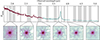 |
Fig. A.1. QSO spectrum (top panel, G235H/F170LP and G395H/F290LP gratings/filters in red and blue, respectively) with examples of the empirical PSF models adopted in our analysis (bottom panels). The wavelength ranges used to compute the PSF are highlighted in grey. |
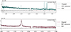 |
Fig. A.2. Example of two PSF-subtracted spectra in the two different gratings for two different sources (G235H/F170LP for C1 and G395H/F290LP for C2, upper and lower panels, respectively). The modelled PSFs in the same aperture of the integrated spectra (see Sect. 3.3) and the PSF-subtracted spectra are shown with dashed black and solid grey lines, respectively. |
Appendix B: Aperture correction results
The aperture correction can be calculated using point source observations from the same instrument and configuration (grating/filter) of our observation. In Sect. 3.3, we used the QSO emission itself to model the PSF from our data. Then, we used this modelling to calculate the wavelength-dependent correction adopting four different apertures of radius 0.2, 0.3, 0.4, and 0.5 arcsec centred on the QSO.
Figure B.1 and Table B.1 show the fraction of the flux at different observed wavelengths normalized to the value obtained in the aperture of 1 arcsec radius, which includes almost the entire emission of the PSF. This fraction decreases when the wavelength increases due to the larger PSF. For an aperture of radius = 0.5 arcsec, the flux lost at the Hβ and Hα wavelengths at redshift z = 4.7 is around 6 % and 8 %, respectively, this value being larger for smaller apertures.
We verified that these results obtained from the continuum also work for the BLR broad Balmer lines. We thus extracted the integrated spectrum of the QSO in two different apertures: R = 0.5″ and 1.0″and modelled the broad Hαwith a Gaussian with a velocity dispersion spanning a range 1000 km s−1> σ > 5000 km s−1, and we also quantified the flux lost in the spectral domain. We found that the integrated flux of the BLR component in both apertures is very similar, with a ratio FBLR(R = 0.5″) / FBLR(R = 1″) = 0.95 (we are losing less than a 5% of the BLR flux in the smallest one). This value is similar to the aperture corrected flux reported in Table B.1 with a value Ffraction (λ = 3.74, R = 0.5″) = 0.92. Then, the values calculated in Table B.1 can be used to correct the integrated spectrum.
 |
Fig. B.1. Fraction of the total flux included in four different apertures (R = 0.2″, 0.3″, 0.4″, and 0.5″) as a function of the observed wavelengths, normalized to the value obtained in the aperture of R = 1″. |
Fraction of total flux included in four different apertures at different observed wavelengths normalized to the value obtained in the aperture of R = 1″.
Appendix C: NIRSpec errors
The errors on the integrated spectrum of a source can be calculated (i) from the error extension present in the data cube in the same spaxels of the selected region propagating them in quadrature; or (ii) considering the spatial noise of our data calculating the root mean square at each wavelength in apertures without source emission.
We calculated the errors using these two methods in three different random apertures (RA1 = 181.3455 deg, Dec1 = –7.7087; RA2 = 181.3460 deg, Dec2 = –7.7079; RA3 = 181.3458 deg, Dec3 = –7.7092). For the G235H grating, the mean error obtained for each method is 0.0065 and 0.0067 × 10⁻²⁰ erg s−1 cm−2 Å−1, respectively. The mean errors in the G395H grating are larger due to the low S/N of the data, 0.025 and 0.022 × 10⁻²⁰ erg s−1 cm−2 Å−1 with method (i) and (ii), respectively. The results of both methods are totally compatible between them according to the mean dispersion of the results in different apertures, then we used the first method to determine the errors in the integrated spectra of the sources within the system.
Appendix D: LAEs and companions
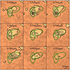 |
Fig. D.1. Channel maps of Hαemission from LAE1. Contours begin at 3σ and are in steps of 5σ. Each channel map covers a FoV of 1″ × 1″ and spans 0.002 μm, which corresponds to 160 km s−1. The green ellipses indicate the location and extension of the two merging galaxies: LAE1a and LAE1b. The emission around these sources is not aligned in the same direction, which discards a rotation scenario. |
Appendix E: Additional candidate galaxies
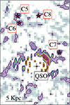 |
Fig. E.1. JWST NIRSpec PSF-subtracted map integrated over the wavelength range 3.635 μm < λ < 3.846 μm, encompassing Hα+[N II] emission lines. The QSO position is marked with a plus symbol. The candidate galaxies found around the QSO are highlighted with stars. |
Coordinates of the additional candidate companion galaxies in BR1202-0725.
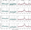 |
Fig. E.2. JWST NIRSpec rest-frame optical spectra (integrated in circular apertures with R = 0.1 arcsec) of the candidate galaxies found around the QSO in the two gratings/filters used (G235H/F170LP and G395H/F290LP; blue and red lines, respectively). The errors in the spectra are shown in light grey. Vertical dashed lines mark the position of the main emission lines in the spectrum at the systemic redshift of the QSO. |
All Tables
Coordinates, redshifts, projected distances from the QSO, velocities, and velocity dispersions of the companion galaxies around the QSO of BR1202-0725.
Emission line observed fluxes (in units of 10−17 erg s−1 cm−2), emission line ratios, and main properties (ionization parameter U, and gas phase metallicity, in terms of oxygen abundance and relative to solar) of the LAEs and confirmed companions, from their integrated spectra reported in Figs. 9 and 11.
Fraction of total flux included in four different apertures at different observed wavelengths normalized to the value obtained in the aperture of R = 1″.
All Figures
|
Fig. 1. HST ACS F775W filter (i-band; left) and JWST NIRSpec IFU Hα(3.74 μm < λ < 3.75 μm; right) image of BR1202-0725. Dust continuum emission from ALMA in Band 7 is shown as black contours. Star symbols illustrate the position of the three LAEs. North is up, east is to the left. A logarithmic colour scale is used. |
| In the text | |
|
Fig. 2. Original (left) and PSF-subtracted (right) maps of the QSO at the wavelength corresponding to the Hβ emission line. |
| In the text | |
|
Fig. 3. JWST/NIRSpec rest-frame optical spectrum of the QSO in the two gratings/filters G235H/F170LP and G395H/F290LP (green and purple lines, respectively), extracted from an aperture of R = 0.5″. The brightest nebular lines are marked and the Fe II multiplet bands are highlighted in grey. The dashed green line shows the broken power-law continuum model fitted to reproduce the featureless continuum emission. The grey line in the bottom panel shows the residuals of the fitting. |
| In the text | |
|
Fig. 4. QSO rest-frame optical continuum-subtracted spectrum (grey line) in the spectral region 4700–5400 Å. The emission lines Hβ and [O III] λλ4959,5007 Å (marked with vertical lines) are blended with the Fe II emission, which can be clearly seen at ∼3 μm. The following fitted Fe II templates are shown: Véron-Cetty et al. (2004, VC+04, red line), Boroson & Green (1992, BG+92, blue line), and Tsuzuki et al. (2006, T+06, yellow line). The lines in the bottom panel show the different residuals of the fitting. |
| In the text | |
|
Fig. 5. Continuum-subtracted JWST NIRSpec spectrum of the QSO. The best-fit model is shown with a solid black line, while the results of the individual components are reported with different colours: the dashed blue line shows the Narrow + Outflow components, and the dotted purple line corresponds to the BLR component. The fitted Véron-Cetty et al. (2004) Fe II template (VC+04) is shown with the dash-dotted orange line. |
| In the text | |
|
Fig. 6. JWST NIRSpec rest-frame optical spectrum of the SMG in the two gratings/filters G235H/F170LP and G395H/F290LP (blue and red lines, respectively), extracted from an aperture of R = 0.3″. The errors of the spectrum are shown in light grey. |
| In the text | |
|
Fig. 7. Comparison of the SMG line profiles of the [O III], Hα+[N II], and [C II] emission lines in velocity space. All line profiles are normalized to their peak value. The vertical dotted black line indicates the zero velocity at the systemic redshift of z = 4.6891 for [O III] λ5007, Hα, and [C II] emission lines. |
| In the text | |
|
Fig. 8. Fitting results for the SMG spectrum, showing the Narrow 1, Narrow 2, BLR, and Outflow components (dotted purple, dashed red, dashed yellow, and dash-dotted blue lines, respectively). The errors considered in the fitting procedure are displayed in grey and the residuals of the fits are shown at the bottom of each panel. Top panel: Fit of the [O III] λλ4959,5007 Å emission lines. The vertical dotted lines mark the position of [O III] at the systemic redshift determined from [C II]. Middle and bottom panels: Fits of the Hα, [N II] λλ6548,6584 Å, and [S II] λλ6717,6731 Å emission lines for the first (outflow) and second (BLR) scenarios described in Sect. 5. The vertical black lines indicate the position of the emission lines for the Narrow 2 component found in [O III]. |
| In the text | |
|
Fig. 9. JWST NIRSpec rest-frame optical spectra of LAE1 and LAE2 in the two gratings/filters used (G235H/F170LP and G395H/F290LP, blue and red lines, respectively), extracted from apertures of R = 0.6″ and 0.3″, respectively. The errors in the spectra are shown in light grey and the kinematic components used to model the emission lines in LAE1 are marked with different curve styles and colours (the two main narrow components are shown with a dashed black and a dotted purple line, respectively, while the broad component is marked shown with a dashed grey line). The spikes that appear in the Hβ emission line of LAE1 are instrumental artefacts; therefore, the measurements of this emission line in LAE1 are not completely reliable. |
| In the text | |
|
Fig. 10. JWST NIRSpec PSF-subtracted maps integrated over the two wavelength ranges reported in each panel, both encompassing [O III] λ5007 Å emission in the same FoV. The QSO position is marked with a plus symbol. The companions found near the QSO are highlighted with red circles, which represent the apertures used to extract their integrated spectra (reported in Fig. 11). |
| In the text | |
|
Fig. 11. JWST NIRSpec rest-frame optical spectra of the four detected companions, C1, C2, C3, and C4, extracted from apertures of R = 0.2″, 0.1″, 0.15″, and 0.1″, respectively. The errors on the spectrum are shown in light grey. The fitting results are shown with a dashed black line. |
| In the text | |
|
Fig. 12. [O III]/Hβ vs [N II]/Hα BPT diagnostic diagram for all objects analysed. The demarcations between H II and AGN-ionized regions (Kauffmann et al. 2003; Kewley et al. 2001, dash-dotted and dashed black lines, respectively) are reported. The vertical lines indicate the [N II]/Hαratio for the two sources for which we do not have values of [O III] and Hβemission lines, with the errors shown by shaded bands (the errors are not visible for the SMG Narrow 1 component). |
| In the text | |
|
Fig. 13. Soft-band (0.5–2 keV) Chandra image of BR1202-0725 (10″ × 10″ box). Data were smoothed with a Gaussian kernel of 2-pixel radius. Circular regions mark the positions of the QSO (blue) and of the SMG (magenta). |
| In the text | |
|
Fig. A.1. QSO spectrum (top panel, G235H/F170LP and G395H/F290LP gratings/filters in red and blue, respectively) with examples of the empirical PSF models adopted in our analysis (bottom panels). The wavelength ranges used to compute the PSF are highlighted in grey. |
| In the text | |
|
Fig. A.2. Example of two PSF-subtracted spectra in the two different gratings for two different sources (G235H/F170LP for C1 and G395H/F290LP for C2, upper and lower panels, respectively). The modelled PSFs in the same aperture of the integrated spectra (see Sect. 3.3) and the PSF-subtracted spectra are shown with dashed black and solid grey lines, respectively. |
| In the text | |
|
Fig. B.1. Fraction of the total flux included in four different apertures (R = 0.2″, 0.3″, 0.4″, and 0.5″) as a function of the observed wavelengths, normalized to the value obtained in the aperture of R = 1″. |
| In the text | |
|
Fig. D.1. Channel maps of Hαemission from LAE1. Contours begin at 3σ and are in steps of 5σ. Each channel map covers a FoV of 1″ × 1″ and spans 0.002 μm, which corresponds to 160 km s−1. The green ellipses indicate the location and extension of the two merging galaxies: LAE1a and LAE1b. The emission around these sources is not aligned in the same direction, which discards a rotation scenario. |
| In the text | |
|
Fig. E.1. JWST NIRSpec PSF-subtracted map integrated over the wavelength range 3.635 μm < λ < 3.846 μm, encompassing Hα+[N II] emission lines. The QSO position is marked with a plus symbol. The candidate galaxies found around the QSO are highlighted with stars. |
| In the text | |
|
Fig. E.2. JWST NIRSpec rest-frame optical spectra (integrated in circular apertures with R = 0.1 arcsec) of the candidate galaxies found around the QSO in the two gratings/filters used (G235H/F170LP and G395H/F290LP; blue and red lines, respectively). The errors in the spectra are shown in light grey. Vertical dashed lines mark the position of the main emission lines in the spectrum at the systemic redshift of the QSO. |
| In the text | |
Current usage metrics show cumulative count of Article Views (full-text article views including HTML views, PDF and ePub downloads, according to the available data) and Abstracts Views on Vision4Press platform.
Data correspond to usage on the plateform after 2015. The current usage metrics is available 48-96 hours after online publication and is updated daily on week days.
Initial download of the metrics may take a while.