| Issue |
A&A
Volume 702, October 2025
|
|
|---|---|---|
| Article Number | A224 | |
| Number of page(s) | 15 | |
| Section | Extragalactic astronomy | |
| DOI | https://doi.org/10.1051/0004-6361/202453298 | |
| Published online | 24 October 2025 | |
MIDIS: Unveiling the star formation history in massive galaxies at 1 < z < 4.5 with spectro-photometric analysis
1
Centro de Astrobiología (CAB), CSIC-INTA, Ctra. de Ajalvir km 4, Torrejón de Ardoz, E-28850 Madrid, Spain
2
Kapteyn Astronomical Institute, University of Groningen, P.O. Box 800 9700 AV Groningen, The Netherlands
3
European Space Agency (ESA), European Space Astronomy Centre (ESAC), Camino Bajo del Castillo s/n, 28692 Villanueva de la Cañada, Madrid, Spain
4
Space Telescope Science Institute, 3700 San Martin Drive, Baltimore, Maryland 21218, USA
5
Max Planck Institut für Astronomie, Königstuhl 17, D-69117 Heidelberg, Germany
6
Department of Astronomy, University of Geneva, Chemin Pegasi 51, 1290 Versoix, Switzerland
7
Department of Astronomy, Oskar Klein Centre, Stockholm University, AlbaNova University Center, 10691 Stockholm, Sweden
8
DTU Space, Technical University of Denmark, Elektrovej 327, 2800 Kgs. Lyngby, Denmark
9
Cosmic Dawn Center (DAWN), Denmark
10
DARK, Niels Bohr Institute, University of Copenhagen, Jagtvej 155A, 2200 Copenhagen, Denmark
11
Centro de Astrobiología (CAB), CSIC-INTA, Camino Bajo del 1166 Castillo s/n, E-28692 Villanueva de la Cañada, Madrid, Spain
12
I. Physikalisches Institut der Universität zu Köln, Zülpicher Str. 77, 50937 Köln, Germany
13
Leiden Observatory, Leiden University, P.O. Box 9513 2300 RA Leiden, The Netherlands
14
European Space Agency, Space Telescope Science Institute, Baltimore, Maryland, USA
15
UK Astronomy Technology Centre, Royal Observatory Edinburgh, Blackford Hill, Edinburgh EH9 3HJ, UK
16
Dept. of Physics and Astronomy, University College London, Gower Street, London WC1E 6BT, United Kingdom
17
Institute of Science and Technology Austria (ISTA), Am Campus 1, 3400 Klosterneuburg, Austria
⋆ Corresponding author.
Received:
4
December
2024
Accepted:
15
August
2025
Abstract
Context. This paper investigates the star formation histories (SFHs) of a sample of massive galaxies (M⋆ ≥ 1010 M⊙) in the redshift range 1 < z < 4.5.
Methods. We analyzed spectro-photometric data, combining broadband photometry from HST and JWST with low-resolution grism spectroscopy from JWST/NIRISS, obtained as part of the MIRI Deep Imaging Survey program. SFHs were derived through spectral energy distribution fitting using two independent codes, BAGPIPES and synthesizer, under various SFH assumptions. This approach enables a comprehensive assessment of the biases introduced by different modeling choices.
Results. The inclusion of NIRISS spectroscopy, even with its low resolution, significantly improves constraints on key physical parameters, such as the mass-weighted stellar age (tM) and formation redshift (zform), by narrowing their posterior distributions. The massive galaxies in our sample exhibit rapid stellar mass assembly, forming 50% of their mass between 3 ≤ z ≤ 9. The highest inferred formation redshifts are compatible with elevated star formation efficiencies (ϵ) at early epochs. Nonparametric SFHs generally imply an earlier and slower mass assembly compared to parametric forms, highlighting the sensitivity of inferred formation timescales to the chosen SFH model–particularly for galaxies at z < 2. We find that quiescent galaxies are, on average, older (tM ∼ 1.1 Gyr) and assembled more rapidly at earlier times than their star-forming counterparts. These findings support the “downsizing” scenario, in which more massive and passive systems form earlier and more efficiently.
Key words: galaxies: evolution / galaxies: formation / galaxies: high-redshift / galaxies: star formation / galaxies: stellar content
© The Authors 2025
 Open Access article, published by EDP Sciences, under the terms of the Creative Commons Attribution License (https://creativecommons.org/licenses/by/4.0), which permits unrestricted use, distribution, and reproduction in any medium, provided the original work is properly cited.
This article is published in open access under the Subscribe to Open model. This email address is being protected from spambots. You need JavaScript enabled to view it. to support open access publication.
1. Introduction
Galaxies are intricate systems typically composed of multiple stellar populations. Observational constraints on their stellar mass assembly provide valuable insights into the physical processes that shape galaxy formation and evolution. Understanding the timescales on which these processes operate is crucial for addressing long-standing questions in galaxy evolution, such as when and how galaxies cease forming stars (i.e., quench; Schawinski et al. 2014; Schreiber 2016; Carnall et al. 2018), and what drives the observed bimodality in galaxy properties (e.g., Whitaker et al. 2012b; Muzzin et al. 2013). In contrast to the hierarchical growth of dark matter halos predicted by Λ cold dark matter models, observations suggest that the stellar components within these halos (i.e., galaxies) grow in a manner that is, at least to some extent, anti-hierarchical or top-down. In particular, the most massive galaxies observed in the local Universe appear to have assembled the bulk of their stellar mass rapidly and were already in place at early cosmic times (Pérez-González et al. 2008b; Marchesini et al. 2010, 2014; Forrest et al. 2020).
The launch of JWST (Gardner 2023) has marked a major leap forward in infrared astronomy, enabling the detection of massive galaxies (> 1010 M⊙) at increasingly earlier epochs (e.g., z > 6; Chworowsky et al. 2024; Shapley et al. 2025). While targeting massive galaxies at high redshift is a powerful way to investigate their formation, this requires deeper observations and limits the sample size. A complimentary approach involves studying such galaxies at lower redshifts and reconstructing their star formation histories (SFHs) through spectral energy distribution (SED) modeling. This method has been shown to provide critical information on the timing of major star formation episodes and the processes that lead to their quenching (e.g., Carnall et al. 2018; Iyer et al. 2019; Tacchella et al. 2022).
However, SEDs are subject to significant and interrelated degeneracies among physical properties such as age, metallicity, and dust attenuation (e.g., Papovich et al. 2001; Lee et al. 2007; Conroy 2013). As a result, photometric observations alone are generally sensitive only to the most recent ∼1 Gyr of star formation, whereas the addition of spectroscopic data can extend sensitivity to earlier epochs (Chaves-Montero & Hearin 2020) and therefore provide key leverage in breaking these degeneracies. This is primarily because spectroscopy offers both emission line and continuum information, each probing different physical processes. Emission lines trace recent or ongoing star formation and nebular conditions (e.g., ionization state and gas metallicity), while the continuum shape and absorption features are sensitive to the underlying stellar populations, dust extinction, and stellar metallicity (e.g., Maraston 2005; Byler et al. 2017). The combination of these components makes it possible to place more accurate constraints on galaxy properties than photometry alone, especially when modeling complex SFHs (e.g., Pacifici et al. 2012).
The advent of large spectroscopic surveys in the local Universe has greatly increased the availability of high signal-to-noise ratio (S/N) continuum spectra, allowing for tighter constraints on galaxy properties (e.g., Pacifici et al. 2012; Thomas et al. 2017). At higher redshifts, however, such high-quality data remained rare prior to JWST. Despite this limitation, several robust trends had been identified. At fixed redshift, lower-mass galaxies consistently host younger stellar populations compared to more massive systems–a phenomenon known as “downsizing” (e.g., Gallazzi et al. 2005, 2014; Pacifici et al. 2016; Carnall et al. 2018). In addition, at fixed stellar mass, the average formation redshift–defined as the redshift at which a galaxy has assembled 50% of its stellar mass–tends to decrease with decreasing observed redshift. This trend likely reflects the combined effects of several mechanisms, including the quenching of newly formed galaxies that join the red sequence (e.g., Brammer et al. 2011; Muzzin et al. 2013; Tomczak et al. 2014), galaxy mergers (e.g., Khochfar & Silk 2009; Khochfar et al. 2011; Emsellem et al. 2011), and episodes of rejuvenated star formation (e.g., Belli et al. 2017). The advent of JWST has finally enabled spectroscopic surveys targeting higher-redshift massive galaxies (e.g., Carnall et al. 2024; Slob et al. 2024).
Despite their advantages, spectroscopic observations are significantly more resource-intensive than photometric ones, particularly when targeting faint, high-redshift galaxies. As a result, spectroscopic samples at early cosmic times have historically been limited in both size and scope. However, in this work, we demonstrate that even low-resolution spectroscopy from the JWST Near Infrared Imager and Slitless Spectrograph (NIRISS; Doyon et al. 2023) provides sufficient spectral coverage and sensitivity to significantly improve constraints on the SFHs of massive galaxies. The low-resolution (R = 150) continuum and emission line information from JWST/NIRISS, together with broadband photometry, enables the robust recovery of key SFH parameters, such as mass-weighted ages and formation redshifts. We took advantage of these spectro-photometric data from JWST/NIRISS, in combination with available broadband and medium-band photometry, to investigate the evolution of massive galaxies in the redshift range 1 < z < 4.5. To this end, we employed state-of-the-art modeling codes by exploring multiple SFHs.
Recent years have seen a significant effort to recover the “true” SFH of galaxies. Traditionally, simple parametric forms have been used to describe it. Among the most commonly used forms is delayed exponentially declining (e.g., Carnall et al. 2019). However, such models often fail to capture the diversity and complexity of galaxy growth, especially at high redshifts. To address this, more sophisticated parametric forms have been introduced. For instance, two-component models, combining an old population (modeled with an exponentially declining SFH) and a recent burst (often described with a double power law), have been successfully employed to model the SFHs of post-starburst galaxies (e.g., Carnall et al. 2018). Recent years have also seen an increase in the use of more flexible methods, such as nonparametric SFHs, which adopt a series of constant star-formation periods, divided into fixed or flexible time intervals (e.g., Iyer et al. 2019; Leja et al. 2019).
In this work we used two state-of-the-art codes: BAGPIPES (Bayesian Analysis of Galaxies for Physical Inference and Parameter Estimation; Carnall et al. 2018) and synthesizer (Pérez-González et al. 2003a) with different assumptions regarding the SFH to describe the evolution of our massive galaxies. The paper is organized as follows: Section 2 describes the NIRISS observations and data reduction process, Sect. 3 outlines our sample selection, Sect. 3.1 details our spectro-photometric modeling approach, and Sect. 4 presents our main results.
Throughout the paper, we assume ΩM = 0.3, Ωλ = 0.7, H0 = 70 kms−1Mpc−1, and AB magnitudes (Gunn et al. 1987).
2. Data description
The analyses in this paper are based on NIRISS data taken in parallel with the MIRI Deep Imaging Survey (MIDIS; Östlin et al. 2025) of the Hubble ultra-deep field (HUDF) conducted by the MIRI European Consortium guaranteed time observations program. Among its many results, MIDIS has played a key role in the discovery of previously undetected faint galaxies (e.g., Pérez-González et al. 2023, 2025), the first little red dot with clear detection of its host galaxy (e.g., Iani et al. 2025; Rinaldi et al. 2025b), and the detailed characterization of the role of the emitter at the epoch of reionization properties of distant galaxies (e.g., Rinaldi et al. 2023, 2024). In addition, MIDIS observations have provided new insights into galaxy morphologies at high redshift (e.g., Boogaard et al. 2024; Costantin et al. 2025).
The NIRISS observations cover a southern portion of the GOODS-S field and consist of 20 h (including overheads) of direct imaging and grism observations in the three bands F115W, F150W, and F200W. This resulted in 1112s,1112s and 2232s on-source direct images in F115W, F150W and F200W, and ∼5.3h grism spectra in each band. These data were reduced using the official JWST pipeline version 1.8.4 (pmap = 1019). In addition to the default pipeline stages, which include snowball correction, we also applied a background homogenization algorithm prior to obtaining the final mosaics, including 1/f- noise removal as in Bagley et al. (2023).
The images were then registered to the same reference frame of the World Coordinate System using the Hubble Legacy Field (HLF) catalog in Whitaker et al. (2019), based on Gaia Data Release 2 (Gaia Collaboration 2016, 2018). In all three images, we then find a median offset of Δα = −0.001 arcsec and Δδ = −0.002 arcsec. We left the pixel scale to the nominal NIRISS pixel scale (0.065″/pixel). The 3σ depth of the direct images observations (measured in circular apertures of 0.2″ diameter) is ∼28.6, 28.7, and 29.1 AB, in F115W, F150W, and F200W, respectively. The 3σ line flux sensitivity of the grism is ∼1.5e − 18 erg s−1cm−2. The MIDIS parallel observations target a region (hereafter MIDIS-P3) of the GOODS-S field covered by the Hubble Space Telescope (HST) ACS and WFC3 from the HLF. In this study we used, in addition to our NIRISS data, the HLF v2 images for all filters from Whitaker et al. (2019). A small portion (∼1/6th) of P3 overlaps with the NIRISS parallel observations of the JWST Extragalactic Medium-band Survey (GO) program JWST Extragalactic (JEMS; PID: 1963; Williams et al. 2023) in the two medium bands F430M and F480M. The NIRISS images from JEMS were reduced in the same way as for the MIDIS images. Figure 1 shows the position of MIDIS-P3 in the GOODS-S field with respect to other JWST programs. It also shows a red-green-blue (RGB) color image of P3 obtained using the three direct images in F115W, F150W, and F200W.
 |
Fig. 1. Image of GOODS-S in H160 from CANDELS. Over-plotted are the regions observed by JWST by different programs, including two of the three pointings of the MIDIS survey in red (P1 and P3). The red insert shows a color composite RGB image of the MIDIS-P3 field obtained using the three direct images in F115W, F150W, and F200W. |
Spectra extraction was performed using the official JWST pipeline. We added an extra step between stage 1 and stage 2 for background removal and homogenization on the 2D grism files. The 2D spectra in stage 2 were extracted in a region that corresponds to the Kron apertures (Kron 1980) identified in Sect. 3.
3. Sample selection
For this work, we selected galaxies previously detected in Cosmic Assembly Near-infrared Deep Extragalactic Legacy Survey (CANDELS Grogin et al. 2011; Koekemoer et al. 2011) with redshift z≥ 1, and stellar masses from Santini et al. 2015 log(M/M⊙)≥10.0. Figure 3 shows the mass and redshift distribution of our targets. Some of the selected galaxies (∼10%) have secure spectroscopic redshift from different works (e.g., Bacon et al. 2023; Santini et al. 2015, and references therein). As P3 is part of the larger Chandra Deep Field South (CDFS), we also checked whether for these galaxies there were any spectra available from the A deen VIMOS survey of the CANDELS UDS and CDES fields collaboration (VANDELS Garilli et al. 2021); however, this was not the case. Our final sample consists of 47 galaxies.
After we identified our galaxy sample, we measured their photometry in the NIRISS images and remeasured their fluxes in the HST ones from HLF by fixing centers, shapes, and sizes to those of the Kron apertures derived for NIRISS. Finally, we cross-matched this catalog to the multi-wavelength catalog from CANDELS in the GOODS-S field (from the Rainbow database1Pérez-González et al. 2008a; Barro et al. 2011) to obtain photometry in the IRAC and MIPS filter (Barro et al. 2011). The final catalog contains photometry in more than 20 filters.
Figure 2 shows the RGB images and NIRISS JHK spectra for a selection of sources in our sample. From both the photometry and the final 1D spectra in the three NIRISS filters, we derived the spectro-photometric redshifts using the eazy-py code (Brammer 2021). As shown in Fig. 3, we have a limited number of objects with independent and secure spectroscopic redshift measurements in our sample (12). With respect to these objects, we obtain a σNMAD = 0.0012 and no outliers (i.e., objects with Δz/(1 + z) > 0.15). Of the objects in our sample without previous redshift measurements, five galaxies have strong, identifiable emission lines (e.g., the top and middle galaxies in Fig. 2). Notably, the most distant galaxy in our redshift sample (z = 4.564 ± 0.001) has been identified through the [O2]λ3727 line. Our redshifts agree very well with the photometric redshifts previously determined from the CANDELS photometry. With respect to previous photometric redshifts, CANDELS redshifts have an outlier fraction (i.e., the fraction of objects with Δz/(1 + z) > 0.15) of 15%.
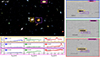 |
Fig. 2. Top left: RGB cutout of P3, centered on one of the galaxies in the sample. The three squares highlight three massive galaxies in the sample. Right: Single GRISM exposure containing the same objects, in the three filters and for one (GR150C) rotation. Bottom left: Extracted spectra with 3σ errors (shaded areas) of the three galaxies. |
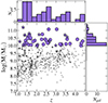 |
Fig. 3. Distribution in mass and redshift from the CANDELS catalog of all galaxies previously detected in P3. Black points are galaxies with photometric redshifts and black crosses galaxies with spectroscopic redshifts. Our selected galaxy sample is shown in purple, with hexagons representing galaxies with photometric redshifts and stars marking galaxies with spectroscopic ones. |
The galaxies in our sample span the redshift range 1.0 ≤ z ≤ 4.5. Figure 4 shows the distribution of our galaxies in the rest-frame U − V versus V − J diagram, hereafter UVJ, as obtained by eazy-py. Most (81%) of our galaxies lies in the star-forming region of the diagram, 19% of them are quiescent.
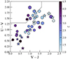 |
Fig. 4. UVJ diagram for the galaxies in our sample color-coded according to their redshift. The size of the points is proportional to the stellar mass. The symbols have the same meaning as in Fig. 3. The line divides the quiescent (top) and star-forming (bottom) parts of the diagram (Whitaker et al. 2012a). |
3.1. Spectro-photometric modeling
After we obtained the spectro-photometric redshifts from eazy-py, we derived galaxy properties through SED-fitting of both photometry and spectroscopy. We decided to use two different codes: BAGPIPES (Carnall et al. 2018) and synthesizer (Pérez-González et al. 2003a). BAGPIPES is a stellar population synthesis modeling package built on the updated BC03 Bruzual & Charlot (2003) spectral library with the 2016 version of the MILES library (Sánchez-Blázquez et al. 2006). It is built on a Kroupa initial mass function (Kroupa 2001) assumption and uses a Multi-Nest nested sampling algorithm (Feroz et al. 2019) to produce posterior distributions of physical parameters. In our run, we also took the resolution NIRISS grism into account. The attenuation law is modeled with Calzetti et al. (2000). For this code, we assumed three different SFHs: a single stellar population described by a delayed-exponential function, a nonparametric SFH and two stellar populations. The two-population model is characterized by an exponential declining model for the old stellar population plus a double power law that describes the more recent bursts of star formation. For the nonparametric SFH we used the continuity model from Leja et al. (2019), which fits directly for Δlog(SFR) between adjacent time bins. This prior explicitly weights against sharp transitions in the star formation rate (SFR) as a function of time. We assumed bins logarithmically spaced from 0 to the age of the Universe at the redshift we observed the object. In the case of two stellar populations, the older component is characterized by a delayed exponential function, while the SFH of the younger component is a burst characterized as a double power law.
The synthesizer code (Pérez-González et al. 2003b, 2008a) assumes a Chabrier initial mass function (Chabrier 2003) with mass limits between 0.1 and 100 M⊙. The attenuation law is modeled with Calzetti et al. (2000). For synthesizer we considered a single stellar population characterized by a delayed exponential SFH, and two stellar populations, characterized by two delayed exponentials.
For BAGPIPES, a summary of the free parameters and their allowed ranges in the SED-fitting procedure for all SED-fitting codes and for the different choice of SFHs is reported in Table 1. For synthesizer, we adopted the same ranges whenever possible. Figure 5 shows the full spectro-photometric modeling of one of the galaxy in our sample.
Free parameters and their allowed ranges used in the SED-fitting procedure for all choices of SFH.
In this work we are interested in when massive galaxies start to assemble their stellar mass, how rapidly they do it, and how rapidly they quench, i.e., their star formation is halted. For this reason, we focused on a subsample of parameters that can be derived from the SED-fitting. These parameters are: stellar mass, SFR, mass-weighted age, the redshift at which the galaxies form 50% of their stellar mass (i.e., formation redshift), and the time and redshifts at which galaxies form a fixed stellar mass (108 − 109 M⊙).
We adopted the surviving mass as the stellar mass throughout this work. We defined the mass-weighted age as follows:
 (1)
(1)
where SFR(t) is the SFR as a function of time. We use the term “formation redshift” (zform) to refer to the redshift corresponding to the mass-weighted age of the galaxy. In particular, first we translated the mass-weighted age to age of the Universe, and from this we identified the formation redshift. This parameter corresponds to the redshift at which a galaxy has assembled 50% of its stellar mass.
To understand how rapidly these galaxies assemble their stellar mass, we used, as an indicator of formation timescale, the time and the redshift at which galaxies have assembled their first 108 and 109 M⊙, respectively (t(108 M⊙), t(109 M⊙), z(108 M⊙), and z(109 M⊙)). The parameters defined above depend on a priori assumptions on SFHs and possibly on the peculiarities of different codes. Table 2 shows the distributions ( ) of the properties discussed in the paper for different classes of galaxies and with all codes. The same convention (
 ) is used throughout the paper. In Appendix A we show how all these parameters compare for the two codes and different SFH assumptions mentioned above.
Average SED-fitting properties of the galaxies in our sample for different codes.
3.2. The fiducial model and the importance of NIRISS low-resolution spectroscopy
To assess which model best matches our data, we began by visually examining the stacked SEDs of quiescent and star-forming galaxies (Fig. 6). Individual SEDs were shifted to the rest-frame before stacking, and the resulting median stack was redshifted to the sample’s average redshift. For quiescent galaxies, the available data do not allow us to clearly distinguish between the different models, as the overall SED shapes and continuum levels are similar across all runs. However, in the case of star-forming galaxies, the right panel of Fig. 6 reveals that neither of the synthesizer runs adequately reproduces the Hα emission lines observed in the NIRISS spectra of a subset of the star-forming sample. This is also evident for the star-forming galaxy in the bottom panels of Fig. 5. These discrepancies suggest that the emission line modeling and/or SFHs implemented in the synthesizer runs are insufficient to capture all spectroscopic features of these galaxies. Consequently, we selected our fiducial models from the BAGPIPES runs, which also allow more flexibility in modeling complex SFHs.
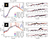 |
Fig. 5. Spectro-photometric SED-fitting of two galaxies (a quiescent and a star-forming one) in our sample. The lines are the best-fit SEDs from different codes and SFH choice. Photometric data are shown as white diamonds. The error bars are smaller than the size of the points. The 1D spectra in F115W, F150W, and F200W are shown in black. The right panels show a zoomed-in view of the spectra in linear scale. The 3σ errors are plotted as shaded grey areas. We report the median S/N of the 1D spectra. |
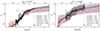 |
Fig. 6. Left: Median SEDs of quiescent galaxies obtained from the different runs, with the shaded regions indicating the 84th–16th percentile range. Overplotted are the stacked low-resolution spectra from NIRISS. Right: Same as the left panel but for star-forming galaxies. All SEDs and spectra are redshifted to the median redshift of the corresponding sample. |
We computed the reduced χ2 values consistently across all model configurations by including both photometric and spectroscopic data in the fits. Among the various runs, the configuration that yields the lowest median reduced χ2 is the BAGPIPES run with two stellar populations. To quantify the relative performance of each model, we computed the median χ2 ratio between each alternative run and the BAGPIPES 2-POP model. The resulting median ratios are 1.04, 2.28, 1.28, and 1.29 for the BAGPIPES 1-POP, BAGPIPES with a nonparametric SFH, synthesizer 1-POP, and synthesizer 2-POP runs, respectively. Based on these results, we adopted the BAGPIPES – 2POP configuration as our fiducial model throughout the remainder of this analysis. For completeness, we also report the results obtained from the BAGPIPES – 1POP and BAGPIPES – nonparametric configurations in the following sections, enabling comparisons and illustrating the impact of model assumptions on the inferred galaxy properties.
To evaluate the specific contribution of the NIRISS spectroscopy to constraining the physical properties of individual galaxies, we performed an additional BAGPIPES – 2POP run using only the photometric data. By comparing these results with those from our fiducial run, we aimed to quantify the added value of the NIRISS spectra. Given our primary interest in understanding the assembly history of stellar mass in galaxies, we focused on the distributions of tM and zform as a function of total formed stellar mass. These distributions, derived from the Bayesian posterior samples provided by BAGPIPES, are shown for two representative galaxies in Fig. 7, which correspond to those previously presented in Fig. 5. Across the entire sample, we find that including the NIRISS spectra results in significantly tighter constraints on the derived parameters, as evidenced by narrower posterior distributions in the tM–mass and zform–mass planes. This tightening of the parameter space reflects the additional information content provided by the spectral data, particularly in terms of emission and absorption line features that are sensitive to recent and intermediate-age star formation. The improvement is clearly visible for the two example galaxies shown in Fig. 7, where the inclusion of spectra leads to a marked reduction in the uncertainty of both stellar mass and formation timescales. The bottom panels of Fig. 7 show that, the best-fit values for stellar mass, tM, and zform shift slightly when spectroscopy is included, although they remain consistent within 1σ with the values derived from the photometry-only runs. This indicates that the spectroscopic data not only improve precision but also validate the overall robustness of the photometric estimates. As a result, we conclude that the addition of NIRISS spectroscopy, even with its low-resolution, enhances our ability to constrain the SFHs of high-redshift galaxies.
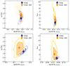 |
Fig. 7. Left: Distribution of tM versus stellar mass derived from the photometry-only run and the fiducial run for the two galaxies (top and bottom) shown in Fig. 5. Right: Same as the left panels but displaying the distribution of zform versus stellar mass. |
4. Results
4.1. Early mass buildup of massive galaxies
According to the fiducial model, the galaxies in our sample have a median stellar mass (and 16th and 84th percentiles) of  , a median redshift of
  , a median mass-weighted age of
  Gyr, and a formation redshift of
  . Moreover, they have assembled 108 M⊙ by redshift
  and 109 M⊙ at redshift
  .
.
Figure 8 shows the formation, quenching, and observed times of the galaxies sample as a function of their stellar mass, according to our fiducial model. We observe a clear downsizing trend, wherein more massive galaxies tend to form and quench earlier in cosmic history. At fixed stellar mass, formation times shift toward higher redshift as stellar mass increases. The only galaxy with mass above 1011 M⊙ that is quenched does so by z ∼ 4. This is consistent with the well-established picture in which massive galaxies undergo rapid early star formation and subsequently quench earlier than their lower-mass counterparts (Carnall et al. 2018; Forrest et al. 2020). Our results align also with the scenario described by Rinaldi et al. (2025a), wherein massive galaxies rapidly establish a self-regulated, steady state of star formation along the main sequence.
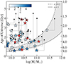 |
Fig. 8. Formation and quenching redshift for our sample as parametrized by BAGPIPES - 2POP. Blueish stars on the y-axis represent the age (and redshift) at which the galaxies form ∼50% of their stellar mass, with the corresponding 50% observed stellar mass on the x-axis. The stars are color-coded according to the redshift of the observation. Red stars indicate the time of quenching and the observed stellar mass. Black circles denote the age of the Universe at the time of the observation for each galaxy (and the corresponding observed stellar mass). These points are connected by solid lines for each galaxy. We also over-plot the maximum observed stellar mass that would be expected for a given star formation efficiency (ϵ). |
In Fig. 8 we also plot the maximum observed stellar mass that would be expected for a given star formation efficiency ϵ. We derived the maximum stellar mass as a function of the redshift for a given ϵ in the NIRISS footprint using the hmf python package (Murray et al. 2013) assuming an SMT fitting function (Sheth et al. 2001). The more reasonable upper limit on the observed stellar mass would use ϵ = 0.2, the maximum inferred from the peak of the stellar mass to halo mass relation across a range of redshifts (Akins et al. 2024). At fixed stellar mass, galaxies that formed at higher redshifts are more compatible with a higher star formation efficiency. This is in agreement with the emerging picture that the assembly of halo and stellar mass has proceeded at different rates throughout cosmic history (e.g., Shuntov et al. 2025).
Figure 9 presents the distribution of SFHs for the full galaxy sample for the three BAGPIPES runs. The median formation redshift results of the the nonparametric run and the fiducial model are very similar (see Table 2). The nonparametric SFH exhibit an earlier onset of stellar mass assembly, with significant star formation already in place by z ∼ 9.6, corresponding to a cosmic time of ∼ 0.52 Gyr. In contrast, the median SFRs in both the one-population and two-population parametric models remain low until z ∼ 7.1, or ∼ 0.75 Gyr after the Big Bang, implying a delay of approximately 230 Myr in the onset of star formation relative to the nonparametric case.
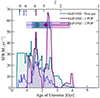 |
Fig. 9. Average SFHs of galaxies in our sample. The shaded areas correspond to the 16th–84th percentile interval computed from the scatter of the SFHs of all galaxies in our sample. The three points on top show the median formation redshifts; the boxes extend to the 16th and 84th percentiles. Solid vertical lines show the median redshift at which these types of galaxies form 108 M⊙ according to the different models, while dashed vertical lines show the median redshift at which these types of galaxies form 109 M⊙. |
We derived the redshifts at which each galaxy reaches a stellar mass of 108 and 109 M⊙, as these quantities are independent of both the redshift of observation and the observed stellar mass. This approach enables a direct comparison with high-redshift studies of the galaxy stellar mass function (e.g., Weibel et al. 2024; Shuntov et al. 2025; Harvey et al. 2025). Using our fiducial model, we computed the comoving number densities of galaxies that have assembled at least 108 M⊙ and 109 M⊙ in stellar mass within the redshift interval 8.5 ≤ z ≤ 9.5. We find number densities of (8.2 ± 2.1) × 10−4 Mpc−3 and (5.8 ± 2.1) × 10−4 Mpc−3, respectively. These values are consistent within 1σ with the stellar mass function estimates at z ∼ 9 from Weibel et al. (2024), who report a number density of ∼ 10−4 Mpc−3 at M∗ ∼ 109 M⊙. Our results also agree with the findings of Harvey et al. (2025), who infer similarly high number densities for galaxies at 108 M⊙ at z > 8.5, suggesting that efficient stellar mass assembly was already underway in a substantial fraction of the population at these early epochs. Furthermore, our inferred densities are in agreement with the abundance of 108 and 109 M⊙ galaxies predicted from clustering and luminosity function modeling in Shuntov et al. (2025). These elevated number densities at high redshift also support the scenario of high star formation efficiencies at z ≥ 9, in agreement with results from recent numerical simulations (Ceverino et al. 2024).
4.2. Trends with redshift
Our galaxy sample spans a wide redshift range, which could potentially dilute some of the observed trends due to evolutionary effects. To mitigate this, we divided the sample into two redshift bins, 1 ≤ z < 2 and z ≥ 2, which approximately correspond to similar intervals in cosmic time. Figure 10 shows the distribution of SFHs for galaxies in each redshift bin, while the median physical properties of the two subsamples are summarized in Table 2.
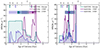 |
Fig. 10. Left: Average SFHs at the lowest redshifts (z < 2). The shaded areas, points, and lines have the same meaning as in Fig. 9. Right: Same as the left panel but for galaxies at higher redshifts (z ≥ 2). |
On average, lower-redshift galaxies have a higher median mass-weighted age of  Gyr and a formation redshift of
  . At these lower redshifts, the difference between nonparametric and parametric SFHs becomes particularly pronounced. Nonparametric SFHs predict that the galaxies reach 108 and 109Msun at higher redshifts. The difference between z8 and z9 is also much higher (see Table 2 for nonparametric models, implying a slower mass assembly.
At higher redshifts, galaxies have a median mass-weighted age of  Gyr and a formation redshift of
  . Interestingly, the differences between nonparametric and parametric SFHs are less pronounced in this redshift regime. The offset in the onset of star formation is smaller, with z8 1.2× larger than the fiducial model. A detailed comparison of all codes and SFH assumptions is presented in Appendix A. At
  , Kaushal et al. (2024) found that nonparametric models derived with Prospector (Leja et al. 2019) generally exhibit more extended SFHs than parametric ones generated with BAGPIPES. A similar trend was reported in Leja et al. (2019) at
  , where nonparametric models consistently produced older stellar ages compared to parametric models from BAGPIPES and other fitting codes. This discrepancy is likely due to differences in how star formation onset is treated: parametric models typically allow the onset time to vary freely, whereas nonparametric models usually assume that star formation begins at t = 0. While previous works have identified similar trends, this is the first time that a consistent comparison is performed using the same fitting code but with different SFH assumptions. Furthermore, we present here the first evidence of a redshift-dependent trend in the divergence between parametric and nonparametric SFHs.
4.3. Trends with star formation activity
We divided our sample into star-forming galaxies and quiescent galaxies on the basis of the SFH of our fiducial model. All galaxies in the quiescent sample are also quiescent according to the UVJ diagram described in Sect. 3. Moreover, they have very low SFRs (averaged over the last 100Myr) according to all the models. Quiescent galaxies have stellar mass of  , mass-weighted age of
  Gyr and formed at
  . Table 2 shows that quiescent galaxies are older with respect to the total and star-forming sample regardless of the choice of SFH or the code used.
Figure 11 shows the average SFH of quiescent galaxies in our sample. According to our fiducial SED model, BAGPIPES - 2 POP, these galaxies assemble the first 108 M⊙ and 109 M⊙ very early in the Universe, with  and
and  , respectively. They also assemble very rapidly, as shown by the small difference between z8 and z9. Our galaxies exhibit different quenching redshifts, i.e., the redshift at which the SFR falls below 10% of the average SFR throughout the galaxy’s history Carnall et al. (2018) as shown in Fig. 8.
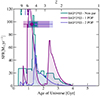 |
Fig. 11. SFHs of quenched galaxies according to different codes and SFHs. The shaded areas, points, and lines have the same meanings as in Fig. 9. |
Unfortunately, we did not have enough quiescent galaxies in our sample to derive their mean properties in different redshift bins. However, in Fig. 12 we plot the formation redshift of our quiescent galaxies as a function of stellar mass and with the points color-coded according to redshift. In the plot, we also show some of the most recent results on the assembly histories of massive quiescent galaxies (e.g., Belli et al. 2019; Carnall et al. 2018; Beverage et al. 2025; Park et al. 2024; Nanayakkara et al. 2025; Slob et al. 2024). The higher redshift galaxies in our sample have a formation redshift of 5 ≲ zform ≲ 9 and a quenching redshift of zquench ∼ 4. The early onset of star formation observed in high-redshift quiescent galaxies indicates that the assembly of massive galaxies in the early Universe occurred at a significantly faster pace compared to their counterparts in the local Universe. Moreover, observations of quiescent galaxies at redshifts up to z ∼ 4 − 5 (e.g., Forrest et al. 2020; Carnall et al. 2023; Setton et al. 2024) indicate that the evolution of the star formation timescale extends to significantly earlier epochs. We do not see any trend between formation redshift and stellar mass in our sample, although with a very limited number of galaxies.
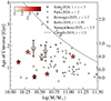 |
Fig. 12. Age of the Universe (left) and the redshift (right) at the time of formation for the quiescent galaxies in the sample as a function of their stellar mass. The symbols are colored by the redshift at observation. We also add several recent results from literature at different redshifts as defined in the legend. |
Star-forming galaxies constitute the dominant population within the studied sample. Figure 13 shows their average SFHs for to different runs. According to our fiducial model, star-forming galaxies have stellar masses of  , mass-weighted ages of
  Gyr. This makes them significantly younger on average compared to quiescent galaxies and form at a slightly later epochs, with
  .
.
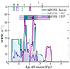 |
Fig. 13. SFHs of star-forming galaxies according to different codes and SFHs. The shaded areas, points, and lines have the same meanings as in Fig. 9. |
5. Conclusions
In this paper we have presented a comprehensive analysis of the SFHs of a mass-complete sample of galaxies with stellar masses ≥1010 M⊙ spanning the redshift range 1 < z < 4.5. Our analysis leveraged a rich set of spectro-photometric data, including broadband photometry and low-resolution grism spectroscopy from JWST/NIRISS, which enabled us to probe the stellar populations of galaxies across cosmic time with improved accuracy. By performing SED-fitting with two modeling codes –BAGPIPES and synthesizer– and employing multiple SFH assumptions (parametric, two-component, andnonparametric forms), we critically assessed how different methodological choices impact the derived formation timescales and assembly histories of massive galaxies. The complete comparison of these modeling approaches is presented in the main text and Appendix A, while in the following we adopt as our fiducial model the results from BAGPIPES using a two-population SFH (see Sect. 3.2). Our main results include:
-
Given the wide redshift range of our sample, we observe substantial diversity in stellar population ages. On average, galaxies in our sample have mass-weighted stellar ages of tM − w ∼ 0.8 Gyr and median formation redshifts of zform ∼ 3.9. These values reflect the fact that even at relatively early cosmic times, massive galaxies had already assembled a substantial portion of their stellar mass.
-
Galaxies assemble rapidly: they formed 108 M⊙ and 109 M⊙ by z8 = 5.9 and z9 = 5.4, respectively.
-
We divided the sample into two redshift bins, 1 ≤ z < 2 and 2 ≤ z ≤ 4.5, and find notable differences in the stellar population properties between the two subsets. Despite having similar stellar masses, the two redshift subsamples trace different evolutionary stages. Galaxies observed at 1 ≲ z < 2 have mass-weighted ages of tM − w ≃ 2.0 Gyr and formed half of their present-day stellar mass by zform ≈ 3.4; this means that several gigayears had therefore elapsed between their main buildup and the epoch of observation. In contrast, galaxies observed earlier, at 2 ≲ z ≲ 4.5, are only tM − w ≃ 0.5 Gyr old, even though their formation redshifts are slightly higher (zform ≈ 4.0). The younger ages simply reflect the much shorter interval (less than a gigayear) between formation and observation. Thus, the apparent age gap arises naturally from look-back time: the farther back we look, the closer each galaxy lies to its own formation epoch.
-
Our analysis highlights that nonparametric SFHs tend to favor earlier formation epochs compared to parametric ones. This is particularly pronounced in the lower-redshift subsample, where the nonparametric model implemented in BAGPIPES predicts that galaxies reach 108 and 109 M⊙ by z8 = 9.8 and z9 = 9.2, respectively–much earlier than in parametric models. These findings emphasize that the choice of SFH parameterization can significantly influence derived formation timescales.
-
Although our sample includes a limited number of quiescent galaxies across the full redshift range, they exhibit systematically older stellar populations (tM − w ∼ 1.1 Gyr) and higher formation redshifts (zform ∼ 4.1) than the star-forming population. While the small number of quiescent systems precludes a detailed statistical analysis, we do observe a tentative trend whereby quiescent galaxies at higher redshifts formed earlier, with formation redshifts reaching as high as zform ∼ 9. These results are qualitatively consistent with the downsizing scenario, in which the most massive and passive systems formed earlier and more rapidly.
-
In contrast, the star-forming galaxies in our sample are typically younger (tM − w ∼ 0.7 Gyr) and formed more recently, with median formation redshifts of zform ∼ 3.8.
 .
.
Acknowledgments
MA acknowledges financial support from Comunidad de Madrid under Atracción de Talento grant 2020-T2/TIC-19971. This work has made use of the Rainbow Cosmological Surveys Database, which is operated by the Centro de Astrobiología (CAB/INTA), partnered with the University of California Observatories at Santa Cruz (UCO/Lick,UCSC). The project that gave rise to these results received the support of a fellowship from the “la Caixa” Foundation (ID 100010434). The fellowship code is LCF/BQ/PR24/12050015. LC acknowledges support from grants PID2022-139567NB-I00 and PIB2021-127718NB-I00 funded by the Spanish Ministry of Science and Innovation/State Agency of Research MCIN/AEI/10.13039/501100011033 and by “ERDF A way of making Europe”. This work is based on observations made with the NASA/ ESA/CSA JWST. The data were obtained from the Mikulski Archive for Space Telescopes (MAST) at the Space Telescope Science Institute, which is operated by the Association of Universities for Research in Astronomy, Inc., under NASA contract NAS 5-03127 for JWST.
References
- Akins, H. B., Casey, C. M., Lambrides, E., et al. 2024, ApJ, submitted, [arXiv:2406.10341] [Google Scholar]
- Bacon, R., Brinchmann, J., Conseil, S., et al. 2023, A&A, 670, A4 [NASA ADS] [CrossRef] [EDP Sciences] [Google Scholar]
- Bagley, M. B., Finkelstein, S. L., Koekemoer, A. M., et al. 2023, ApJ, 946, L12 [NASA ADS] [CrossRef] [Google Scholar]
- Barro, G., Pérez-González, P. G., Gallego, J., et al. 2011, ApJS, 193, 30 [Google Scholar]
- Barro, G., Pérez-González, P. G., Cava, A., et al. 2019, ApJS, 243, 22 [NASA ADS] [CrossRef] [Google Scholar]
- Belli, S., Newman, A. B., & Ellis, R. S. 2017, ApJ, 834, 18 [Google Scholar]
- Belli, S., Newman, A. B., & Ellis, R. S. 2019, ApJ, 874, 17 [Google Scholar]
- Beverage, A. G., Slob, M., Kriek, M., et al. 2025, ApJ, 979, 249 [Google Scholar]
- Boogaard, L. A., Gillman, S., Melinder, J., et al. 2024, ApJ, 969, 27 [NASA ADS] [CrossRef] [Google Scholar]
- Brammer, G. 2021, gbrammer/eazy-py: Tagged release 2021 (Zenodo) [Google Scholar]
- Brammer, G. B., Whitaker, K. E., van Dokkum, P. G., et al. 2011, ApJ, 739, 24 [NASA ADS] [CrossRef] [Google Scholar]
- Bruzual, G., & Charlot, S. 2003, MNRAS, 344, 1000 [NASA ADS] [CrossRef] [Google Scholar]
- Byler, N., Dalcanton, J. J., Conroy, C., & Johnson, B. D. 2017, ApJ, 840, 44 [Google Scholar]
- Calzetti, D., Armus, L., Bohlin, R. C., et al. 2000, ApJ, 533, 682 [NASA ADS] [CrossRef] [Google Scholar]
- Carnall, A. C., McLure, R. J., Dunlop, J. S., & Davé, R. 2018, MNRAS, 480, 4379 [Google Scholar]
- Carnall, A. C., Leja, J., Johnson, B. D., et al. 2019, ApJ, 873, 44 [Google Scholar]
- Carnall, A. C., McLure, R. J., Dunlop, J. S., et al. 2023, Nature, 619, 716 [NASA ADS] [CrossRef] [Google Scholar]
- Carnall, A. C., Cullen, F., McLure, R. J., et al. 2024, MNRAS, 534, 325 [NASA ADS] [CrossRef] [Google Scholar]
- Ceverino, D., Nakazato, Y., Yoshida, N., Klessen, R. S., & Glover, S. C. O. 2024, A&A, 689, A244 [NASA ADS] [CrossRef] [EDP Sciences] [Google Scholar]
- Chabrier, G. 2003, PASP, 115, 763 [Google Scholar]
- Chaves-Montero, J., & Hearin, A. 2020, MNRAS, 495, 2088 [NASA ADS] [CrossRef] [Google Scholar]
- Chworowsky, K., Finkelstein, S. L., Boylan-Kolchin, M., et al. 2024, AJ, 168, 113 [NASA ADS] [CrossRef] [Google Scholar]
- Conroy, C. 2013, ARA&A, 51, 393 [NASA ADS] [CrossRef] [Google Scholar]
- Costantin, L., Gillman, S., Boogaard, L. A., et al. 2025, A&A, 699, A360 [NASA ADS] [CrossRef] [EDP Sciences] [Google Scholar]
- Doyon, R., Willott, C. J., Hutchings, J. B., et al. 2023, PASP, 135, 098001 [NASA ADS] [CrossRef] [Google Scholar]
- Emsellem, E., Cappellari, M., Krajnovic, D., et al. 2011, MNRAS, 414, 888 [NASA ADS] [CrossRef] [Google Scholar]
- Feroz, F., Hobson, M. P., Cameron, E., & Pettitt, A. N. 2019, Open J. Astrophys., 2, 10 [Google Scholar]
- Forrest, B., Marsan, Z. C., Annunziatella, M., et al. 2020, ApJ, 903, 47 [NASA ADS] [CrossRef] [Google Scholar]
- Gaia Collaboration (Prusti, T., et al.) 2016, A&A, 595, A1 [NASA ADS] [CrossRef] [EDP Sciences] [Google Scholar]
- Gaia Collaboration (Brown, A. G. A., et al.) 2018, A&A, 616, A1 [NASA ADS] [CrossRef] [EDP Sciences] [Google Scholar]
- Gallazzi, A., Charlot, S., Brinchmann, J., White, S. D. M., & Tremonti, C. A. 2005, MNRAS, 362, 41 [Google Scholar]
- Gallazzi, A., Bell, E. F., Zibetti, S., Brinchmann, J., & Kelson, D. D. 2014, ApJ, 788, 72 [Google Scholar]
- Gardner, J. 2023, APS Meeting Abstracts, 2023, A01.001 [Google Scholar]
- Garilli, B., McLure, R., Pentericci, L., et al. 2021, A&A, 647, A150 [NASA ADS] [CrossRef] [EDP Sciences] [Google Scholar]
- Grogin, N. A., Kocevski, D. D., Faber, S. M., et al. 2011, ApJS, 197, 35 [NASA ADS] [CrossRef] [Google Scholar]
- Gunn, J. E., Emory, E. B., Harris, F. H., & Oke, J. B. 1987, PASP, 99, 518 [Google Scholar]
- Harvey, T., Conselice, C. J., Adams, N. J., et al. 2025, ApJ, 978, 89 [NASA ADS] [CrossRef] [Google Scholar]
- Iani, E., Rinaldi, P., Caputi, K. I., et al. 2025, ApJ, 989, 160 [Google Scholar]
- Iyer, K. G., Gawiser, E., Faber, S. M., et al. 2019, ApJ, 879, 116 [NASA ADS] [CrossRef] [Google Scholar]
- Kaushal, Y., Nersesian, A., Bezanson, R., et al. 2024, ApJ, 961, 118 [NASA ADS] [CrossRef] [Google Scholar]
- Khochfar, S., & Silk, J. 2009, MNRAS, 397, 506 [NASA ADS] [CrossRef] [Google Scholar]
- Khochfar, S., Emsellem, E., Serra, P., et al. 2011, MNRAS, 417, 845 [Google Scholar]
- Koekemoer, A. M., Faber, S. M., Ferguson, H. C., et al. 2011, ApJS, 197, 36 [NASA ADS] [CrossRef] [Google Scholar]
- Kron, R. G. 1980, ApJS, 43, 305 [Google Scholar]
- Kroupa, P. 2001, MNRAS, 322, 231 [NASA ADS] [CrossRef] [Google Scholar]
- Lee, J. C., Kennicutt, R. C., Funes, J. G. S., Sakai, S., & Akiyama, S. 2007, ApJ, 671, L113 [Google Scholar]
- Leja, J., Carnall, A. C., Johnson, B. D., Conroy, C., & Speagle, J. S. 2019, ApJ, 876, 3 [Google Scholar]
- Maraston, C. 2005, MNRAS, 362, 799 [NASA ADS] [CrossRef] [Google Scholar]
- Marchesini, D., Whitaker, K. E., Brammer, G., et al. 2010, ApJ, 725, 1277 [NASA ADS] [CrossRef] [Google Scholar]
- Marchesini, D., Muzzin, A., Stefanon, M., et al. 2014, ApJ, 794, 65 [NASA ADS] [CrossRef] [Google Scholar]
- Murray, S. G., Power, C., & Robotham, A. S. G. 2013, Astron. Comput., 3, 23 [CrossRef] [Google Scholar]
- Muzzin, A., Marchesini, D., Stefanon, M., et al. 2013, ApJ, 777, 18 [NASA ADS] [CrossRef] [Google Scholar]
- Nanayakkara, T., Glazebrook, K., Schreiber, C., et al. 2025, ApJ, 981, 78 [Google Scholar]
- Östlin, G., Pérez-González, P. G., Melinder, J., et al. 2025, A&A, 696, A57 [NASA ADS] [CrossRef] [EDP Sciences] [Google Scholar]
- Pacifici, C., Charlot, S., Blaizot, J., & Brinchmann, J. 2012, MNRAS, 421, 2002 [Google Scholar]
- Pacifici, C., Kassin, S. A., Weiner, B., Charlot, S., & Gardner, J. P. 2016, ApJ, 832, 79 [Google Scholar]
- Pacifici, C., Iyer, K. G., Mobasher, B., et al. 2023, ApJ, 944, 141 [NASA ADS] [CrossRef] [Google Scholar]
- Papovich, C., Dickinson, M., & Ferguson, H. C. 2001, ApJ, 559, 620 [NASA ADS] [CrossRef] [Google Scholar]
- Park, M., Belli, S., Conroy, C., et al. 2024, ApJ, 976, 72 [Google Scholar]
- Pérez-González, P. G., Gil de Paz, A., Zamorano, J., et al. 2003a, MNRAS, 338, 508 [CrossRef] [Google Scholar]
- Pérez-González, P. G., Gil de Paz, A., Zamorano, J., et al. 2003b, MNRAS, 338, 525 [Google Scholar]
- Pérez-González, P. G., Rieke, G. H., Villar, V., et al. 2008a, ApJ, 675, 234 [Google Scholar]
- Pérez-González, P. G., Trujillo, I., Barro, G., et al. 2008b, ApJ, 687, 50 [CrossRef] [Google Scholar]
- Pérez-González, P. G., Costantin, L., Langeroodi, D., et al. 2023, ApJ, 951, L1 [CrossRef] [Google Scholar]
- Pérez-González, P. G., Östlin, G., Costantin, L., et al. 2025, ApJ, accepted, [arXiv:2503.15594] [Google Scholar]
- Rinaldi, P., Caputi, K. I., Costantin, L., et al. 2023, ApJ, 952, 143 [NASA ADS] [CrossRef] [Google Scholar]
- Rinaldi, P., Caputi, K. I., Iani, E., et al. 2024, ApJ, 969, 12 [NASA ADS] [CrossRef] [Google Scholar]
- Rinaldi, P., Navarro-Carrera, R., Caputi, K. I., et al. 2025a, ApJ, 981, 161 [Google Scholar]
- Rinaldi, P., Pérez-González, P. G., Rieke, G. H., et al. 2025b, ApJ, submitted, [arXiv:2504.01852] [Google Scholar]
- Sánchez-Blázquez, P., Peletier, R. F., Jiménez-Vicente, J., et al. 2006, MNRAS, 371, 703 [Google Scholar]
- Santini, P., Ferguson, H. C., Fontana, A., et al. 2015, ApJ, 801, 97 [Google Scholar]
- Schawinski, K., Urry, C. M., Simmons, B. D., et al. 2014, MNRAS, 440, 889 [Google Scholar]
- Schreiber, C., Elbaz, D., Pannella, M., et al. 2016, A&A, 589, A35 [NASA ADS] [CrossRef] [EDP Sciences] [Google Scholar]
- Setton, D. J., Khullar, G., Miller, T. B., et al. 2024, ApJ, 974, 145 [Google Scholar]
- Shapley, A. E., Sanders, R. L., Topping, M. W., et al. 2025, ApJ, 981, 167 [Google Scholar]
- Sheth, R. K., Mo, H. J., & Tormen, G. 2001, MNRAS, 323, 1 [NASA ADS] [CrossRef] [Google Scholar]
- Shuntov, M., Ilbert, O., Toft, S., et al. 2025, A&A, 695, A20 [NASA ADS] [CrossRef] [EDP Sciences] [Google Scholar]
- Slob, M., Kriek, M., Beverage, A. G., et al. 2024, ApJ, 973, 131 [Google Scholar]
- Tacchella, S., Conroy, C., Faber, S. M., et al. 2022, ApJ, 926, 134 [NASA ADS] [CrossRef] [Google Scholar]
- Thomas, D., Maraston, C., Schawinski, K., et al. 2017, MNRAS, 472, 2872 [Google Scholar]
- Tomczak, A. R., Quadri, R. F., Tran, K.-V. H., et al. 2014, ApJ, 783, 85 [Google Scholar]
- Weibel, A., Oesch, P. A., Barrufet, L., et al. 2024, MNRAS, 533, 1808 [NASA ADS] [CrossRef] [Google Scholar]
- Whitaker, K. E., Kriek, M., van Dokkum, P. G., et al. 2012a, ApJ, 745, 179 [CrossRef] [Google Scholar]
- Whitaker, K. E., van Dokkum, P. G., Brammer, G., & Franx, M. 2012b, ApJ, 754, L29 [Google Scholar]
- Whitaker, K. E., Ashas, M., Illingworth, G., et al. 2019, ApJS, 244, 16 [CrossRef] [Google Scholar]
- Williams, C. C., Tacchella, S., Maseda, M. V., et al. 2023, ApJS, 268, 64 [NASA ADS] [CrossRef] [Google Scholar]
Appendix A: Dependence of results on a priori assumptions and fitting techniques
In this section we describe the robustness of the different parameters that can be obtained from the SED-fitting analysis. To understand better the differences shown in Table 2, we compare the parameters obtained in the different runs against the value of the "fiducial" model. Throughout this work, we used the BAGPIPES - 2 POP run as our fiducial model.
A.1. Stellar masses
The mass differences of log(M*/M*, fiducial), with respect to the fiducial mass, are shown in Fig. A.1. Over the entire mass range, the median differences between the mass obtained with different codes and the fiducial mass is up to ∼0.1 dex for all runs. This is consistent with previous comparisons between different codes (e.g., Leja et al. 2019; Pacifici et al. 2023). As expected, stellar mass is a well-constrained parameter that can be recovered by different codes and different assumptions. There are not any observable trends, either with stellar masses or with different codes.
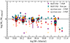 |
Fig. A.1. Stellar mass differences (in log) for the different SFH models and the different codes with respect to the fiducial one. Smaller points are individual galaxies, and bigger points with the error bars are the median obtained in each bin. The bins have been chosen to contain the same number of galaxies. Shaded regions represent 1σ errors. |
A.2. Mass-weighted ages and formation redshifts
Figure A.2 shows the comparison between the mass-weighted ages and formation redshifts of the different codes and assumptions against the fiducial model. Over the entire sample, both BAGPIPES and synthesizer with a delayed−τ model, predicts smaller mass-weighted ages than the fiducial model. This difference is on the order of ∼ 47% forBAGPIPES - 1 POP and ∼65% for synthesizer - 1 POP. This is consistent with the fact that single population models might be biased toward the youngest stars, which can overshine the more evolved stellar population. Synthesizer - 2 POP predicts a difference in mass weighted ages of 12% with respect to the fiducial model, the lowest difference between our runs. As our fiducial model is the BAGPIPES with two populations, this suggest that the assumptions on the SFH are more important than the intrinsic differences from different codes. BAGPIPES - nonparametric also agrees very well with the fiducial model, with an average difference of 26%.
Formation redshifts take into account the different redshifts at which our galaxies are observed. From Fig. A.2, we observe similar trends as for the mass-weighted ages. However, this parameter is better constrained. BAGPIPES - 1 POP gives Δzform/(1 + zform) of ∼ 11%, while synthesizer - 1 POP of ∼ 13%. Synthesizer - 2 POP has the better agreement with the fiducial model, with Δzform/(1 + zform of ∼ of 3% over the whole sample. A good agreement (Δzform/(1 + zform ∼ -5%) is found also for BAGPIPES - nonparametric.
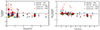 |
Fig. A.2. Left: Relative difference between the mass-weighted ages derived by the different codes with respect to the fiducial one. Right: Same as the left panel but for the formation redshift. In both panels, smaller points are individual galaxies, and bigger points with the error bars are the median obtained in each bin. The bins have been chosen to contain the same number of galaxies. |
A.3. Formation timescales
In order to compare how rapidly our galaxies form stars, we derived the times at which the galaxies formed their first 108M⊙ and 109M⊙. Figure A.3 shows the comparison between t(108 M⊙) and t(109 M⊙) versus the fiducial model. Also in this case, the best agreement is between synthesizer - 2 POP and the fiducial model with a median difference of 9% and 1% for t8 and t9. A 15% difference in t8 is found for BAGPIPES - nonparametric, but with a much larger scatter. The two single population models from BAGPIPES and synthesizer consistently predicts lower t8 and t9, with a difference of ∼ 60% for BAGPIPES and ∼ 70% synthesizer. Figure A.4 shows the same results as in Fig. A.3 but in terms of redshift. While the formation redshift of the galaxy is mostly independent on the choice of SFH and for different codes, A.4 shows that when a nonparametric SFH is considered, galaxies start to assemble their stellar mass at earlier epochs. The discrepancy between nonparametric SFHs and the parametric models is particularly evident at low z8 and z9. On average, BAGPIPES- nonparametric has Δz8/(1 + z8) of ∼ 40% and Δz9/(1 + z9) of 34% with respect to the fiducial model.
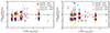 |
Fig. A.3. Left: Relative difference between the time at which the galaxy assembles its first 108M⊙ with respect to the fiducial one (synthesizer - 2 POP). Right : same as left panel but for t(109 M⊙). In both panels, smaller points are individual galaxies, bigger points with the error bars are the median obtained in each bin. The bins have been chosen to contain the same number of galaxies. |
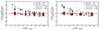 |
Fig. A.4. Left panel: Relative difference between the redshift at which the galaxy assemble 108M⊙ with respect to the fiducial one (synthesizer - composite). Right panel: Same as the left panel but for z9. In both panels, smaller points are individual galaxies, and bigger points with the error bars are the median obtained in each bin. The bins have been chosen to contain the same number of galaxies. |
A.4. Star formation rate
We derived the SFR averaged over the last 100 Myrs with the different prescriptions for the SED-fitting. Figure A.5, shows the comparison between all models and the SFR derived from UV and mid-IR data (Barro et al. 2019), in this case the “true” SFR. BAGPIPES - 1 POP and BAGPIPES - 2 POP underestimate the true SFR by a factor of 40%. BAGPIPES - nonparametric underestimates the true SFR by a factor of 13%. Synthesizer - 1 POP underestimates the true SFR by a factor of 10%. Synthesizer - 2 POP is the only model that overestimates the true SFR by a factor of 49%.
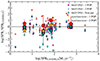 |
Fig. A.5. SFR differences (in log) for the different SFH models and that estimated from the combination of UV and mid-IR data. Smaller points are individual galaxies, and bigger points with the error bars are the median obtained in each bin. The bins have been chosen to contain the same number of galaxies. |
All Tables
Free parameters and their allowed ranges used in the SED-fitting procedure for all choices of SFH.
Average SED-fitting properties of the galaxies in our sample for different codes.
All Figures
|
Fig. 1. Image of GOODS-S in H160 from CANDELS. Over-plotted are the regions observed by JWST by different programs, including two of the three pointings of the MIDIS survey in red (P1 and P3). The red insert shows a color composite RGB image of the MIDIS-P3 field obtained using the three direct images in F115W, F150W, and F200W. |
| In the text | |
|
Fig. 2. Top left: RGB cutout of P3, centered on one of the galaxies in the sample. The three squares highlight three massive galaxies in the sample. Right: Single GRISM exposure containing the same objects, in the three filters and for one (GR150C) rotation. Bottom left: Extracted spectra with 3σ errors (shaded areas) of the three galaxies. |
| In the text | |
|
Fig. 3. Distribution in mass and redshift from the CANDELS catalog of all galaxies previously detected in P3. Black points are galaxies with photometric redshifts and black crosses galaxies with spectroscopic redshifts. Our selected galaxy sample is shown in purple, with hexagons representing galaxies with photometric redshifts and stars marking galaxies with spectroscopic ones. |
| In the text | |
|
Fig. 4. UVJ diagram for the galaxies in our sample color-coded according to their redshift. The size of the points is proportional to the stellar mass. The symbols have the same meaning as in Fig. 3. The line divides the quiescent (top) and star-forming (bottom) parts of the diagram (Whitaker et al. 2012a). |
| In the text | |
|
Fig. 5. Spectro-photometric SED-fitting of two galaxies (a quiescent and a star-forming one) in our sample. The lines are the best-fit SEDs from different codes and SFH choice. Photometric data are shown as white diamonds. The error bars are smaller than the size of the points. The 1D spectra in F115W, F150W, and F200W are shown in black. The right panels show a zoomed-in view of the spectra in linear scale. The 3σ errors are plotted as shaded grey areas. We report the median S/N of the 1D spectra. |
| In the text | |
|
Fig. 6. Left: Median SEDs of quiescent galaxies obtained from the different runs, with the shaded regions indicating the 84th–16th percentile range. Overplotted are the stacked low-resolution spectra from NIRISS. Right: Same as the left panel but for star-forming galaxies. All SEDs and spectra are redshifted to the median redshift of the corresponding sample. |
| In the text | |
|
Fig. 7. Left: Distribution of tM versus stellar mass derived from the photometry-only run and the fiducial run for the two galaxies (top and bottom) shown in Fig. 5. Right: Same as the left panels but displaying the distribution of zform versus stellar mass. |
| In the text | |
|
Fig. 8. Formation and quenching redshift for our sample as parametrized by BAGPIPES - 2POP. Blueish stars on the y-axis represent the age (and redshift) at which the galaxies form ∼50% of their stellar mass, with the corresponding 50% observed stellar mass on the x-axis. The stars are color-coded according to the redshift of the observation. Red stars indicate the time of quenching and the observed stellar mass. Black circles denote the age of the Universe at the time of the observation for each galaxy (and the corresponding observed stellar mass). These points are connected by solid lines for each galaxy. We also over-plot the maximum observed stellar mass that would be expected for a given star formation efficiency (ϵ). |
| In the text | |
|
Fig. 9. Average SFHs of galaxies in our sample. The shaded areas correspond to the 16th–84th percentile interval computed from the scatter of the SFHs of all galaxies in our sample. The three points on top show the median formation redshifts; the boxes extend to the 16th and 84th percentiles. Solid vertical lines show the median redshift at which these types of galaxies form 108 M⊙ according to the different models, while dashed vertical lines show the median redshift at which these types of galaxies form 109 M⊙. |
| In the text | |
|
Fig. 10. Left: Average SFHs at the lowest redshifts (z < 2). The shaded areas, points, and lines have the same meaning as in Fig. 9. Right: Same as the left panel but for galaxies at higher redshifts (z ≥ 2). |
| In the text | |
|
Fig. 11. SFHs of quenched galaxies according to different codes and SFHs. The shaded areas, points, and lines have the same meanings as in Fig. 9. |
| In the text | |
|
Fig. 12. Age of the Universe (left) and the redshift (right) at the time of formation for the quiescent galaxies in the sample as a function of their stellar mass. The symbols are colored by the redshift at observation. We also add several recent results from literature at different redshifts as defined in the legend. |
| In the text | |
|
Fig. 13. SFHs of star-forming galaxies according to different codes and SFHs. The shaded areas, points, and lines have the same meanings as in Fig. 9. |
| In the text | |
|
Fig. A.1. Stellar mass differences (in log) for the different SFH models and the different codes with respect to the fiducial one. Smaller points are individual galaxies, and bigger points with the error bars are the median obtained in each bin. The bins have been chosen to contain the same number of galaxies. Shaded regions represent 1σ errors. |
| In the text | |
|
Fig. A.2. Left: Relative difference between the mass-weighted ages derived by the different codes with respect to the fiducial one. Right: Same as the left panel but for the formation redshift. In both panels, smaller points are individual galaxies, and bigger points with the error bars are the median obtained in each bin. The bins have been chosen to contain the same number of galaxies. |
| In the text | |
|
Fig. A.3. Left: Relative difference between the time at which the galaxy assembles its first 108M⊙ with respect to the fiducial one (synthesizer - 2 POP). Right : same as left panel but for t(109 M⊙). In both panels, smaller points are individual galaxies, bigger points with the error bars are the median obtained in each bin. The bins have been chosen to contain the same number of galaxies. |
| In the text | |
|
Fig. A.4. Left panel: Relative difference between the redshift at which the galaxy assemble 108M⊙ with respect to the fiducial one (synthesizer - composite). Right panel: Same as the left panel but for z9. In both panels, smaller points are individual galaxies, and bigger points with the error bars are the median obtained in each bin. The bins have been chosen to contain the same number of galaxies. |
| In the text | |
|
Fig. A.5. SFR differences (in log) for the different SFH models and that estimated from the combination of UV and mid-IR data. Smaller points are individual galaxies, and bigger points with the error bars are the median obtained in each bin. The bins have been chosen to contain the same number of galaxies. |
| In the text | |
Current usage metrics show cumulative count of Article Views (full-text article views including HTML views, PDF and ePub downloads, according to the available data) and Abstracts Views on Vision4Press platform.
Data correspond to usage on the plateform after 2015. The current usage metrics is available 48-96 hours after online publication and is updated daily on week days.
Initial download of the metrics may take a while.