| Issue |
A&A
Volume 702, October 2025
|
|
|---|---|---|
| Article Number | A75 | |
| Number of page(s) | 9 | |
| Section | Stellar structure and evolution | |
| DOI | https://doi.org/10.1051/0004-6361/202453373 | |
| Published online | 09 October 2025 | |
Mass-radius relation of white dwarfs from close binary systems
1
Instituto de Astrofísica de La Plata, IALP, CCT-CONICET-UNLP, La Plata, Argentina
2
Facultad de Ciencias Astronómicas y Geofísicas de La Plata, Paseo del Bosque s/n, (1900) La Plata, Argentina
⋆ Corresponding author: This email address is being protected from spambots. You need JavaScript enabled to view it.
Received:
10
December
2024
Accepted:
9
August
2025
Abstract
Context. The mass-radius relation (MRR) of white dwarf (WD) stars is a fundamental issue. It has been studied and improved from its original version given by S. Chandrasekhar in 1931. The MRR represents a powerful tool to interpret observations of these compact objects. Originally, it was studied by constructing zero-temperature models. After that, many studies were performed considering finite temperature effects, improved versions of the equation of state, and relativistic effects.
Aims. The main goal of this paper is to build an MRR employing models of WDs obtained through the evolution of close binary systems (CBSs). This scenario allows for the formation of low-mass helium white dwarfs, thus permitting an extension of the MRR to the low-mass range. On the other hand, our models provide a detailed orbital evolution of the systems, which adds an important ingredient to take into account.
Methods. We computed the evolution of a set of CBSs composed by a normal solar-composition donor star together with a compact object (a neutron star or a black hole) that undergo stable mass transfer. We cover a range of initial masses of the donor between 0.50 and 7.00 M⊙ and initial orbital periods from 0.5 to 10 days. For the accreting compact objects we consider a neutron star of 1.40 M⊙ or a black hole of 4.0, 6.0, 8.0, or 10.0 M⊙.
Results. We find that, as expected, WDs with moderate or high masses (M > 0.5 M⊙) follow a monotonic MRR with a radius decreasing as a function of its mass and as the objects cool down. However, this monotonic behavior does not occur in the case of low-mass objects, especially in those with rather high effective temperatures, between 30 and 60 kK (1 kK = 103 K). This is so because the outermost hydrogen layer, whose mass fraction depends on the details of the previous evolution, occupies a non-negligible fraction of the stellar radius.
Conclusions. The MRR of intermediate or high-mass WDs (M > 0.4 M⊙) formed by binary evolution shows the expected behavior and is in agreement with the MRRs previously presented by other authors. Moreover, this MRR looks similar to that of WDs coming from isolated evolution: the radius of the star decreases as the object cools down. We extended the MRR to the region of low-mass WDs, namely, to masses as low as 0.16 M⊙. Notably, the MRR no longer has a univocal behavior at this point. That is, for a given effective temperature, we obtained models with different values of mass for the same radius. Our analysis shows that the position of a remnant on the MRR at the beginning of the cooling track heavily depends on the details of its previous evolution. Therefore, at M < 0.40 M⊙, for a given mass and effective temperature, there is a wide range of possible radii. This should not be overlooked when using the MRR for low mass WDs.
Key words: binaries: close / stars: evolution / white dwarfs
Fellow of the Consejo Nacional de Investigaciones Científicas y Técnicas (CONICET), Argentina.
Member of the Carrera del Investigador Científico, CONICET, Argentina.
Member of the Carrera del Investigador Científico, Comisión de Investigaciones Científicas de la Provincia de Buenos Aires (CIC), Argentina.
© The Authors 2025
 Open Access article, published by EDP Sciences, under the terms of the Creative Commons Attribution License (https://creativecommons.org/licenses/by/4.0), which permits unrestricted use, distribution, and reproduction in any medium, provided the original work is properly cited.
This article is published in open access under the Subscribe to Open model. This email address is being protected from spambots. You need JavaScript enabled to view it. to support open access publication.
1. Introduction
After the landmark paper by Chandrasekhar (1935), the relation between the mass and the radius of white dwarf (WD) stars has been widely studied. A mass-radius relation (MRR) can be established throughout the life of a star, but notably in the case of WDs, it is highly reliable due to the well-known physical processes that occur at the very end of the evolution of low and intermediate mass stars. Chandrasekhar assumed that the WD is a non-rotating spherically symmetric object in hydrostatic equilibrium with a zero temperature Fermi-Dirac gas of non-interacting electrons and a homogeneous chemical composition. Chandrasekhar’s MRR predicts that the radius of a WD is smaller the more massive the object is and that there exists a limiting mass above which hydrostatic equilibrium is no longer possible (MCh = 1.4 M⊙). Considering a polytropic stellar model with non-relativistic degenerate electrons, the MRR is given by  , where RWD and MWD are the radius and the mass of the WD, respectively. This is a good approximation for the case of low and intermediate-mass WDs. This relation was improved by Hamada & Salpeter (1961). Their work considered an equation of state of degenerated electrons still at zero temperature but including corrections to Chandrasekhar’s approach. They incorporated Coulomb, Thomas-Fermi, and exchange corrections (see Salpeter 1961 for further details). They also included realistic chemical compositions (see Figure 1 in that paper).
Theoretical studies based on more realistic WD models at a finite temperature have been performed to depict the MRR. Panei et al. (2000) computed a detailed WD MRR for various internal compositions by performing a cooling evolution starting from models at luminosities far larger than the WD regime. Though plausible, these initial models were not derived from fully evolutionary calculations. Fontaine et al. (2001) assumed a constant hydrogen layer thickness in all models regardless of progenitor and WD mass. The more recent studies of Romero et al. (2013, 2019) made clear that the mass of the hydrogen layer takes an important role in the resulting MRR and that it depends on the mass of the remnant. In Romero et al. (2019), the authors made detailed evolutionary calculations to investigate the dependence of the MRR on the mass of the hydrogen layer of WDs. For that purpose, they computed a set of full evolutionary models of progenitor stars with stellar masses between 0.9 M⊙ and 6.6 M⊙, which resulted in C-O core WDs with masses between 0.493 M⊙ and 1.05 M⊙, and then studied the impact of the hydrogen envelope content on the radius (and log10(g)) at a fixed stellar mass. They found a direct correlation between the radius and the hydrogen mass content: higher hydrogen masses lead to greater radii.
The MRR of WDs is affected by the presence of rotation and/or magnetic fields, as shown long ago by Ostriker & Hartwick (1968). The early developments of these effects were reviewed by Shapiro & Teukolsky (1983). Due to their importance, the effects continue to be studied to this day. Franzon & Schramm (2015) considered extreme regimes of both rotation and magnetic fields together with the effects due to general relativity. They found a possible existence of super-Chandrasekhar objects up to 2.09 M⊙ that may be progenitors of superluminous Type Ia supernovae. More recently, the impact of magnetic fields on the MRR was revisited by Gupta et al. (2020). The authors were interested in the lack of detection of such super-Chandrasekhar objects and showed that the luminosity of these objects can be suppressed enough so that they are hardly detectable.
Observations of WDs using different techniques have confirmed the general characteristics of the theoretical MRR. In the empirical studies performed by Schmidt (1996), the author calculated the masses and radii of a large number of WDs using the best values for parallaxes and gravitational redshifts available at that time. The author obtained the radius via the surface brightness method and the mass from gravitational redshift. Provencal et al. (1998) obtained revised estimates for the mass and radius of 21 WDs (isolated or in binary systems) using data from the Hipparcos survey and found values that are in agreement with the theoretical MRR models of Wood (1995). Holberg et al. (2012) studied the orbital evolution of WD members of binary systems to obtain their masses and then applied photometric and spectroscopic techniques to determine the radius of the WD. They used models from Wood (1995), and their estimates favored models of CO core WDs with thick H envelopes of 10−4 M⊙ above 30 kK. Parsons et al. (2017) obtained mass and radius estimates for WDs from eclipsing binaries, and with other WDs studied in previous works (O’Brien et al. 2001; Parsons et al. 2010, 2012a,b,c, 2016; Pyrzas et al. 2012; Bours et al. 2014), they tested the theoretical MRR models of Benvenuto & Althaus (1999) and Fontaine et al. (2001), finding good agreement between the measurements and the theoretical predictions. Joyce et al. (2018) used parallaxes from Gaia DR2 with spectroscopy from HST and FUSE to calculate the mass and radius of 11 WDs. They claim that most of them are consistent with the theoretical results of Fontaine et al. (2001). McGill et al. (2023) performed semi-empirical studies using astrometric microlensing events between an isolated WD and a distant background source, from which the mass of the WD was inferred and then compared with theoretical predictions. Their results are in agreement with the MRR and cooling tracks of theoretical CO core WDs. Recently, Arseneau et al. (2024) used wide binaries with direct measurements of gravitational redshift to test the MRR of WDs with main-sequence companions, obtaining an MRR consistent with the relationship presented in Fontaine et al. (2001). Finally, Karinkuzhi et al. (2024) tested the MRR for magnetized WDs, estimating the mass by comparing its location in the Hertzsprung-Russell (HR) diagram with evolutionary tracks from Gupta et al. (2020) for different masses (assuming its core composition). The authors obtained a good fit at lower surface magnetic fields and predicted super-Chandrasekhar WDs at higher magnetic fields.
Remarkably, a systematic study of the MRR for WDs descending from close binary systems (CBSs) has not been performed yet. The importance of considering this family of WDs is supported by different motives. First, if we can calculate the orbital evolution of the system, we can access one of the best observable parameters in astronomy: the orbital period. Second, it is in binary systems that the best estimates of the mass of a star can be obtained. On the other hand, the existence of low-mass helium white dwarfs (He-WDs) can only be explained within the framework of close binary evolution. For an isolated star to reach the state of a He-WD, it must have had a mass low enough that the helium core does not exceed ∼0.45 M⊙1. Due to its low mass, the time it would take for a He-WD progenitor to reach this state under isolated conditions is greater than the age of the Universe. However, low-mass He-WDs have been reported from observations since the second half of the past century (see Table 1 in Bergeron et al. 1992). The formation channel for these WDs must be binary (see, e.g., Podsiadlowski et al. 2002; Benvenuto & De Vito 2004). Finally, a WD produced in a CBS loses an important fraction of its hydrogen mass in the mass transfer episode(s)–as much as 75% of its mass. Since the MRR depends on the hydrogen envelope mass (Romero et al. 2019), this requires a detailed study of the WD descendants from CBSs. Detailed evolutionary models in which the mass transfer rate is calculated naturally provide a more physically plausible approach to the hydrogen mass content for these WDs.
The aim of this paper is to construct a complete grid that allows us to study the MRR of WDs resulting from CBSs. The models presented here extend the MRR to low-mass He-WDs with masses as small as 0.16 M⊙. Furthermore, the detailed calculation of the donor (WD progenitor) mass loss rate in CBSs from our models consistently provides the hydrogen mass of the donor. This leads to a more realistic analysis of its impact on the MRR. Our CBSs consist of a solar composition zero age main sequence donor star and an already formed accreting compact object, either a neutron star (NS) or a black hole (BH), with an orbital period short enough so that mass transfer episodes can occur. Since this is a general introductory work on the subject, we considered neither the effects of rotation nor those of magnetic fields in our calculations because they are relevant only in extreme cases, namely, cases of very fast rotators (with rotational periods of the order of tens of seconds) and/or of intense magnetic fields (∼1014 G). In this set of calculations we also neglected the occurrence of winds at stages of high luminosities and effective temperatures (Krtička et al. 2020). These winds have a minor effect on the MRR we present in this paper.
This paper is organized as follows. In Sect. 2 we describe our numerical tool (Sect. 2.1) employed in our simulations and define the simulations we performed (Sect. 2.2). In Sect. 3 we present and analyze the results obtained from our simulations. Finally, in Sect. 4, we present the main conclusions of this work.
2. The calculations
2.1. The evolutionary code
To compute the models presented in this paper, we employed our close binary evolutionary code presented in Benvenuto & De Vito (2003), De Vito & Benvenuto (2012) and Benvenuto et al. (2014). If the system is in a detached state, the code solves the structure of the donor as if it were isolated and calculates the evolution of the orbit and the value of the radius of the Roche lobe for each step. When a Roche-lobe overflow (RLOF) episode begins, the code implicitly solves the donor star structure; the mass-transfer rate,  ; both masses; and the orbital semi-axis. It includes detailed and updated physical ingredients fully described in De Vito & Benvenuto (2012) and references therein. Convective regions are treated using mixing length theory, with a mixing length parameter of αML = 1.55 in all our models. We considered that the NSs and BHs in our models can accrete a fraction, β, of the material coming from the donor star. As usual, in close binary evolutionary models, β is a free parameter, which has a constant value throughout the calculations. In this paper we consider β = 0.5 for all models (see, e.g., Podsiadlowski et al. 2002). Angular momentum losses are due to gravitational radiation, magnetic braking, and mass loss from the system and have been treated as in Benvenuto & De Vito (2003). The mass transfer rate was calculated employing the Ritter (1988) and Kolb & Ritter (1990) prescriptions, and we considered the mass loss by winds from the donor star as in Reimers (1975), with an efficiency of the wind of η = 1 (for a more detailed description, see Echeveste et al. 2024).
2.2. The models
We computed a grid of binary evolution calculations considering accreting NSs with an initial mass value of 1.4 M⊙ and BHs with initial masses of 4.0, 6.0, 8.0, and 10.0 M⊙. Both accretors were considered point masses, and the accretion rate was limited in each case by the corresponding Eddington limit. We assumed solar metallicity (X = 0.721, Z = 0.014) donor stars with initial masses ranging from 0.50 to 4.00 M⊙ in the case of an NS companion and from 1.0 to 7.0 M⊙ in the case of a BH companion. The initial orbital period ranged from 0.50 days to 10 days in all cases. We note that the restriction of the initial mass of the donor in the case of NS companions was employed because donors heavier than 4.00 M⊙ lead to very high mass transfer rates (≳10−2 M⊙/yr) and unstable episodes of mass loss and the subsequent development of common envelope conditions. In order to compare our results with those obtained by Romero et al. (2019), we included BH accretors. This gave us the possibility of obtaining heavier WDs because we could consider more massive donor stars, keeping a mass ratio of q ≲ 1 and therefore a stable mass transfer throughout the calculation.
Detailed calculations of the evolution of the donor stars were performed from the zero age main sequence until the end of the objects’ evolution as a WD with a very low luminosity (log10(L/L⊙) = − 5) or until the object acquired a very low mass value (0.05 M⊙) or an age of 14 Gyr. The grid of calculations consists of a total of 1046 models. Of these, 637 have an NS and 409 have a BH companion.
3. Results
3.1. Main results
In Figure 1 we present the MRR obtained from our grid of models. Although the main part of our analysis is based on the final cooling tracks2 of the donor stars in this subsection, we remark that there are different possible radii of the stars for the same mass due to the occurrence of hydrogen thermonuclear flashes (TNFs) in low-mass objects. This is discussed in Section 3.2. From Figure 1, the dependence of the MRR with the effective temperature of the models can be seen. As expected, the stellar radius is larger if the stellar mass (effective temperature) is smaller (higher). This relation is so because, for lower masses, outer layers are not strongly degenerated, and hence, the pressure dependence on the temperature is not negligible. This in turn makes the star undergo a stronger swelling the higher the effective temperature is. For WDs with masses higher than ≈0.5 M⊙, there is a monotonic ordering of the models: the lower the effective temperature, the smaller the stellar radius. This monotonic behavior does not occur in lower-mass WDs. In fact, as we discuss below, there are cases in which objects with a given radius and effective temperature have masses that are appreciably different. This is a consequence of the occurrence of TNFs, RLOFs, and nuclear burning before entering the final WD cooling track.
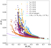 |
Fig. 1. Mass-radius relation of our WD models obtained from close binary evolution. The colors indicate different effective temperatures along the final cooling track, ranging from 10 kK to 60 kK. Circles (squares) correspond to He (CO)-core WDs. Hamada-Salpeter curves at zero temperature with different chemical compositions are plotted for comparison. |
To quantitatively analyze this behavior, we selected a series of models, which we define in Table 1 and present in Figure 2. In the left panel, we show the evolution of the remnants as the effective temperature decreases (in the vertical downward direction). We defined the hydrogen mass content by
 (1)
(1)
Initial parameters of the selected models.
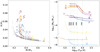 |
Fig. 2. Mass-radius relation with selected WDs highlighted from 50 kK downward (left panel), and hydrogen mass vs. effective temperature (right panel). The dots correspond to their values at 10, 20, 30, 40, and 50 kK, and each color corresponds to a different WD. The two figures use the same color code. Labels correspond to the notation of Table 1. The hydrogen depletion is due to residual nuclear burning along the final cooling track. |
where X is the hydrogen abundance by mass and dm is the mass element. The right panel of Figure 2 depicts the evolution of the hydrogen mass content of the donor (due to late nuclear burning) with the effective temperature for each model. We note that in these evolutionary stages, the hydrogen mass content is located entirely in the outermost layers. Each point over the curves indicates the effective temperature denoted in the left panel for each model (from 50 kK to 10 kK). The color code is the same as in the left panel. It is clear from this figure that it is not trivial to make general correlations between the hydrogen mass content, the mass of the WD, and the effective temperature of the remnant. In its simplest version, the MRR gives the mass of a WD if we have its radius and vice versa. More recent and updated models show the complexity of the MRR, even in the case of isolated progenitors. However, in Figure 13 of Romero et al. (2019), it is possible to see a well-defined behavior of the MRR when the hydrogen mass content is varied. This behavior is nicely reproduced by our models in the more massive range (M ≥ 0.45 M⊙) of the WDs (as shown in Figure 1). However, for lower-mass WDs (whose existence is explained only through close binary evolution models), the MRR widens without a trend that can be highlighted at first glance, making it non-trivial to establish some general relationship between the mass of the WD, its effective temperature, hydrogen mass content, and the radius of the object. As the temperature decreases, the MRR narrows, as can be seen in Figure 5.
To further explore this behavior, we selected two pairs of models from Table 1: model B and model E (PAIR-1); model A and model C (PAIR-2). For each pair, the two models have the same luminosity at Teff = 50 kK, as can be seen in the left panels of Figures 3 and 4. The dots in the HR diagrams denote the effective temperature considered in Figure 2. At Teff = 50 kK, the remnants of the donors have almost the same radius for each pair, as can be seen in the left panel of Figure 2. However, the value of the masses are not the same, with a difference of ΔM = 0.0569 M⊙ for PAIR-1 and ΔM = 0.0547 M⊙ for PAIR-2 (see Table 2). In the right panel of Figures 3 and 4, we show the evolution of the hydrogen mass content for each model of the selected pairs.
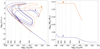 |
Fig. 3. Left panel: Hertzsprung-Russell diagram of the two stars corresponding to PAIR-1, which have the same luminosity at an effective temperature of 50 kK. The dots correspond to 10, 20, 30, 40, and 50 kK. Dashed lines represent fast parts of the tracks (see main text). The model names (Table 1) are shown and are consistent in color with their corresponding curve in Figure 2. Right panel: Hydrogen mass vs. effective temperature for the same models. |
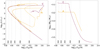 |
Fig. 4. Same as Figure 3 but for PAIR-2. The dots correspond to 10, 20, 30, 40, and 50 kK, respectively. Dashed lines represent fast parts of the tracks (see main text). The model names, according to Table 1, are shown and are consistent in color with their corresponding curve in Figure 2. |
Selected models at Teff = 50 kK.
Regarding PAIR-1, the hydrogen mass content of model B is always higher than in model E. This can be understood by looking at the evolution of the donors of PAIR-1 in the left panel of Figure 3. Once the first and longest episode of mass loss ends3, the donor goes to the left in the HR diagram, towards the high effective temperature region, and begins to experience a cooling path. If the hydrogen-rich envelope is massive enough and the temperature at its base is hot enough, the star can undergo a TNF. In this episode, a fraction of the remaining hydrogen is burnt to helium, reducing the hydrogen content of the envelope. The star is forced to swell suddenly, and its radius may reach its corresponding Roche lobe radius, leading to a late RLOF episode, where some further hydrogen-rich layers are lost. Afterward, the star evolves blueward again, and if its remaining hydrogen content is high enough, it may undergo a subsequent TNF. If this is not the case, the star enters the final cooling track. These late mass loss episodes (if any) have a minor impact on the hydrogen content of the envelope. As can be seen in the left panel of Figure 3, model B experiences only one TNF, whereas model E experiences four. It is important to remark that in model B, the first mass transfer episode begins on the red giant branch, while in model E, this occurs when the donor star is still on the main sequence. That is, their evolutionary paths are notably different.
Considering PAIR-2, we note that the lightest donor, corresponding to model A, undergoes a TNF, while the donor in model C does not. The occurrence of the TNF leaves the donor in model A with less hydrogen mass content at the beginning of the cooling track than the component of model C (see right panel of Figure 4). Notably, the difference in the hydrogen content in this pair is not as big as in the case of PAIR-1 at the same evolutionary stage. At effective temperatures between 30 and 20 kK, the remnant of model C develops residual hydrogen burning in its envelope, notably diminishing its hydrogen content to values lower than that of model A’s remnant.
These examples show that in the case of WDs coming from CBSs, the hydrogen content of the WD progenitor when entering the final cooling track is largely determined by its previous evolution and that it heavily influences its position on the MRR. The impact of the hydrogen content on the envelope of a WD in the position of the MRR was previously studied by Romero et al. (2019) in the case of isolated and more massive WDs (M ≳ 0.5 M⊙). The dependence on the thickness of the hydrogen envelope content is less critical in this mass range. However, as the WD mass decreases, the hydrogen content of the envelope depends more strongly on the previous binary evolution. Therefore, the initial masses of the components, the initial orbital period, the presence of TNFs, the mass loss episodes induced by them (if they occur), and the residual nuclear burning significantly all affect the hydrogen content of the WD.
In Figure 5 we present the MRR at the different values of effective temperature considered in the previous analysis (from 60 kK to 10 kK). A normalized color bar is included, denoting the hydrogen content. We note that not all the simulated systems allow the donor to reach effective temperatures greater than 40 kK, so the number of WDs plotted is not the same in all panels of the figure. In addition, some WDs cool down so slowly that they do not reach effective temperatures as low as 10 kK at an age less than that of the Universe. In fact, from our grid of 1046 models, 823 reach 10 kK, 603 reach 20 kK, 519 reach 30 kK, 497 reach 40 kK, 401 reach 50 kK, and 298 reach 60 kK. We also note that since the models with the highest hydrogen mass content do not reach effective temperatures as high as 30 kK, they appear only in the three lower panels of Figure 5.
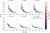 |
Fig. 5. Color map of the hydrogen mass for the MRR obtained at different effective temperatures, from 10 kK to 60 kK. Theoretical curves from Panei et al. (2000) are plotted for comparison. The green (dashed) lines correspond to Helium WDs of (from left to right) 4.0, 8.0, 12.0, 16.0, and 20.0 kK with the same hydrogen layer. The light blue (point-dashed) lines correspond to carbon WDs of (from left to right) 5.0, 15.0, 25.0, 35.0, 45.0, 55.0, 70.0, 85.0, and 100.0 kK with the same hydrogen and helium layers. |
As can be seen from Figure 5, at hotter effective temperatures, the MRR is not univocally determined since there can be a difference in mass of up to ≈0.05 M⊙ for the same radius. This spread arises from the fact that previous binary evolution modifies the resulting outer structure of the WD, and this effect is especially relevant at the very beginning of the final WD cooling track (see the right panel of Figure 2). At lower effective temperatures, this spread narrows as the WD has spent enough time on the final cooling track because of the still active residual nuclear burning. While each WD reaches the final cooling track at a different Teff–hindering direct panel-to-panel comparisons unless the data are constrained–we note that at a fixed Teff, WDs with higher hydrogen masses exhibit larger radii.
Finally, we compared our results with those obtained by Romero et al. (2019). In that paper, the authors explored the dependence of the MRR on the hydrogen content of the WDs. For that purpose, they employed models corresponding to isolated progenitors with masses between 0.95 and 6.6 M⊙ and a metallicity of Z = 0.01. The resulting CO WDs have masses between ∼0.493 and 1.05 M⊙. The different masses of the hydrogen content of their models come from the prescriptions adopted for the evolution along the asymptotic giant branch or from adding some mass to the proto-WD from a binary companion. We find that the MRR obtained from our calculations overlaps fairly well with those of Romero et al. (2019) in the entire region of the MRR explored by both sets of calculations.
3.2. Analyzing the possibility that the remnants are not on the final cooling track
Most of our previous analysis in this paper has been based on results corresponding to models when they attain effective temperatures of 50, 40, 30, 20, and 10 kK on the final cooling track. As can be seen in Figures 3 and 4, a fraction of the considered donor stars undergo one or more TNFs, while others do not. In Figure 3, the donor star of model B reaches each of these temperatures twice but only once as a WD on the final cooling track. In Figure 4 one can see that model A suffers one TNF, while model C does not have any TNFs. The donor of model A reaches 50 and 40 kK twice, 30 kK four times, 20 kK eight times, and 10 kK six times. Only a few of these cases do not correspond to a WD structure at all and/or represent an evolutionary stage that is too fast4 to have a significant chance to be observed. We consider it remarkable that once reaching a local maximum effective temperature and bending downward up to TNF, the donor of model A spends ≈77 Myr at this stage. Therefore, it is possible and probable to detect stars in these conditions.
In the left panel of Figure 6 we show the mass and radius of the donor from model A when it reaches Teff = 30 and 20 kK before the TNF (squares) and compare it with its values on the final cooling track (circles). Since for a given effective temperature there is no obvious observational way to deduce on which part of the track a WD is, this adds a further spread in the MRR, thus leading to an additional uncertainty when using it for low-mass objects.
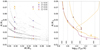 |
Fig. 6. Left panel: Mass-radius relation with PAIR-2 highlighted. The dots correspond to the mass and radius values given by our models at 10, 20, 30, 40, and 50 kK, while squares represent other possible values (at 20 and 30 kK) if the WD is not on the final cooling track. Right panel: Radius of the donor star as a function of the effective temperature for PAIR-2. Dashed lines represent fast parts of the tracks. The dots correspond to remnants on the final cooling track, while squares show other possible radii that could be observed for the same object at 20 and 30 kK. |
In the right panel of Figure 6, we show the radius of the donor stars corresponding to models A and C as a function of the effective temperature. There, dashed lines correspond to very fast, hardly detectable parts of the tracks. When the donor of model A reaches Teff = 30 kK, it has a radius of 0.0542 R⊙, which is 46.5% larger than its radius when it is at the same effective temperature but on the final cooling track (0.0370 R⊙; see left panel of Figure 4). If interpreted as a WD on the final cooling track, a radius of 0.0542 R⊙ would correspond to an appreciably lighter object (≈10% in mass). At Teff = 20 kK, the same situation occurs twice, but the differences in radii are smaller (0.0348 R⊙ and 0.0369 R⊙, which are 15.2% and 22.1% larger than the final cooling track radius of 0.0302 R⊙, respectively). Due to its complexity, we defer a detailed analysis of this problem to a future publication.
3.3. Observational sample
To test the MRR obtained from our simulations, we selected 26 WDs belonging to binary systems with good estimates of the masses, radii, effective temperatures, and orbital period of the systems. These characteristic values and the corresponding references are shown in Table 3. The sample consists of WDs that belong to different kinds of binaries: double WDs and pre-cataclysmic systems. This last group is composed by a WD and a low-mass (usually M type) companion that would have emerged from a common envelope episode (Paczynski 1976; Knigge et al. 2011). The orbital periods associated with pre-cataclysmics are of some hours, leading to a mass transfer episode in which the WD is going to be the accretor and the companion is its donor star. In the group presented in Table 3, some WDs are clearly identified as a He-WD or a CO-WD, but in other cases the chemical composition of the WD cannot be determined because of the value of its mass (∼0.45 M⊙). On the other hand, in many cases, it is not possible to estimate the hydrogen content of the WDs. In Figure 7, we plot the theoretical MRR from our models and the observational data presented in Table 3. Notably, we find that not only do the observed WDs lie within our results of the MRR, but their effective temperature is similar to the simulated WDs that appear near them in the MRR.
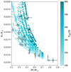 |
Fig. 7. Mass-radius relation of simulated WDs from close binary evolution at different effective temperatures, from 10 kK to 60 kK. Circles correspond to He-core WDs, while squares are CO-core WDs. We include observational data represented with squares with their corresponding error bars (see Table 3). |
4. Conclusions
In this paper, we have revisited the classical problem of the MRR of WDs. We did so by performing calculations of their formation in close binary systems with mass transfer. The models were computed from the zero age main sequence to its final stage as a WD. We considered NS and BH companions to expand our grid of donor masses while keeping mass transfer episodes stable. This choice should not be regarded as restrictive for the application of our results. Indeed, we remark that the MRR of massive WDs we computed overlaps with the results presented in Romero et al. (2013, 2019) (see last paragraph of Section 3.1).
We find that our models are in agreement with the well-known monotonic behavior of the MRR for intermediate and high-mass WDs. For WDs with M ≳ 0.45 M⊙, the MRR does not show a dependence on the particular structure of the close binary systems from which they have evolved. Quite contrarily, in the case of low-mass WDs (0.15 M⊙ ≲ M ≲ 0.45 M⊙), the MRR is much more complex than would be expected from less realistic models. This is even more important when these WDs have rather high effective temperatures of a few 104 K.
We selected a sample of WDs belonging to binary systems with observational estimates for their masses, radii, and effective temperatures. When considering the sets of results corresponding to the effective temperatures that bracket that of the observed object, we find in all cases that the mass and radius of the object fall on the computed MRR within the spread of the MRR described above. Thus, our results correctly represent the observational data.
Data availability
A set of tables containing the relevant information (mass, radius, luminosity, surface gravity and hydrogen mass of the WD, final mass of the accreting object, and orbital period of the system) for our simulated WDs at different effective temperatures is both available at doi.10.5281/zenodo.16985927 and at handle.net/11336/263461. For further information or a specific simulation, please contact the authors.
This is the threshold mass of a star’s He core that is able to reach a temperature high enough to ignite He burning (∼108 K).
The final cooling track is defined as the path followed by the star in the HR diagram from the point of maximum effective temperature value to its final state as a WD.
We note that some systems experience only this episode of mass loss.
Here, we considered fast parts of the evolutionary track to those in which the star changes its position in the HR diagram more than 2% in 1000 years.
Acknowledgments
We acknowledge our anonymous referee for his/her corrections that largely helped us to improve the original version of the present paper.
References
- Arseneau, S., Chandra, V., Hwang, H.-C., et al. 2024, ApJ, 963, 17 [NASA ADS] [Google Scholar]
- Benvenuto, O. G., & Althaus, L. G. 1999, MNRAS, 303, 30 [Google Scholar]
- Benvenuto, O. G., & De Vito, M. A. 2003, MNRAS, 342, 50 [NASA ADS] [CrossRef] [Google Scholar]
- Benvenuto, O. G., & De Vito, M. A. 2004, MNRAS, 352, 249 [NASA ADS] [CrossRef] [Google Scholar]
- Benvenuto, O. G., De Vito, M. A., & Horvath, J. E. 2014, ApJ, 786, L7 [NASA ADS] [CrossRef] [Google Scholar]
- Bergeron, P., Saffer, R. A., & Liebert, J. 1992, ApJ, 394, 228 [NASA ADS] [CrossRef] [Google Scholar]
- Bours, M. C. P., Marsh, T. R., Parsons, S. G., et al. 2014, MNRAS, 438, 3399 [NASA ADS] [CrossRef] [Google Scholar]
- Chandrasekhar, S. 1935, MNRAS, 95, 207 [NASA ADS] [CrossRef] [Google Scholar]
- De Vito, M. A., & Benvenuto, O. G. 2012, MNRAS, 421, 2206 [NASA ADS] [CrossRef] [Google Scholar]
- Echeveste, M., Novarino, M. L., Benvenuto, O. G., & De Vito, M. A. 2024, MNRAS, 530, 4277 [NASA ADS] [CrossRef] [Google Scholar]
- Fontaine, G., Brassard, P., & Bergeron, P. 2001, PASP, 113, 409 [NASA ADS] [CrossRef] [Google Scholar]
- Franzon, B., & Schramm, S. 2015, Phys. Rev. D, 92, 083006 [NASA ADS] [CrossRef] [Google Scholar]
- Gupta, A., Mukhopadhyay, B., & Tout, C. A. 2020, MNRAS, 496, 894 [Google Scholar]
- Hamada, T., & Salpeter, E. E. 1961, ApJ, 134, 683 [NASA ADS] [CrossRef] [Google Scholar]
- Holberg, J. B., Oswalt, T. D., & Barstow, M. A. 2012, AJ, 143, 68 [NASA ADS] [CrossRef] [Google Scholar]
- Joyce, S. R. G., Barstow, M. A., Casewell, S. L., et al. 2018, MNRAS, 479, 1612 [NASA ADS] [Google Scholar]
- Karinkuzhi, D., Mukhopadhyay, B., Wickramasinghe, D., & Tout, C. A. 2024, MNRAS, 529, 4577 [CrossRef] [Google Scholar]
- Knigge, C., Baraffe, I., & Patterson, J. 2011, ApJS, 194, 28 [Google Scholar]
- Kolb, U., & Ritter, H. 1990, A&A, 236, 385 [NASA ADS] [Google Scholar]
- Krtička, J., Kubát, J., & Krtičková, I. 2020, A&A, 635, A173 [NASA ADS] [CrossRef] [EDP Sciences] [Google Scholar]
- McGill, P., Anderson, J., Casertano, S., et al. 2023, MNRAS, 520, 259 [NASA ADS] [CrossRef] [Google Scholar]
- O’Brien, M. S., Bond, H. E., & Sion, E. M. 2001, ApJ, 563, 971 [Google Scholar]
- Ostriker, J. P., & Hartwick, F. D. A. 1968, ApJ, 153, 797 [Google Scholar]
- Paczynski, B. 1976, IAU Symp., 73, 75 [NASA ADS] [Google Scholar]
- Panei, J. A., Althaus, L. G., & Benvenuto, O. G. 2000, A&A, 353, 970 [Google Scholar]
- Parsons, S. G., Marsh, T. R., Copperwheat, C. M., et al. 2010, MNRAS, 407, 2362 [NASA ADS] [CrossRef] [Google Scholar]
- Parsons, S. G., Marsh, T. R., Gänsicke, B. T., et al. 2012a, MNRAS, 419, 304 [Google Scholar]
- Parsons, S. G., Marsh, T. R., Gänsicke, B. T., et al. 2012b, MNRAS, 420, 3281 [NASA ADS] [Google Scholar]
- Parsons, S. G., Gänsicke, B. T., Marsh, T. R., et al. 2012c, MNRAS, 426, 1950 [Google Scholar]
- Parsons, S. G., Hill, C. A., Marsh, T. R., et al. 2016, MNRAS, 458, 2793 [NASA ADS] [CrossRef] [Google Scholar]
- Parsons, S. G., Gänsicke, B. T., Marsh, T. R., et al. 2017, MNRAS, 470, 4473 [Google Scholar]
- Podsiadlowski, P., Rappaport, S., & Pfahl, E. D. 2002, ApJ, 565, 1107 [NASA ADS] [CrossRef] [Google Scholar]
- Provencal, J. L., Shipman, H. L., Høg, E., & Thejll, P. 1998, ApJ, 494, 759 [NASA ADS] [CrossRef] [Google Scholar]
- Pyrzas, S., Gänsicke, B. T., Brady, S., et al. 2012, MNRAS, 419, 817 [NASA ADS] [CrossRef] [Google Scholar]
- Reimers, D. 1975, in Problems in Stellar Atmospheres and Envelopes, eds. B. Baschek, W. H. Kegel, & G. Traving, 229 [Google Scholar]
- Ritter, H. 1988, A&A, 202, 93 [NASA ADS] [Google Scholar]
- Romero, A. D., Kepler, S. O., Córsico, A. H., Althaus, L. G., & Fraga, L. 2013, ApJ, 779, 58 [NASA ADS] [CrossRef] [Google Scholar]
- Romero, A. D., Kepler, S. O., Joyce, S. R. G., Lauffer, G. R., & Córsico, A. H. 2019, MNRAS, 484, 2711 [NASA ADS] [Google Scholar]
- Salpeter, E. E. 1961, ApJ, 134, 669 [NASA ADS] [CrossRef] [Google Scholar]
- Schmidt, H. 1996, A&A, 311, 852 [NASA ADS] [Google Scholar]
- Shapiro, S. L., & Teukolsky, S. A. 1983, Black Holes, White Dwarfs and Neutron Stars. The Physics of Compact Objects (New York: Wiley) [Google Scholar]
- Wood, M. A. 1995, White Dwarfs (Berlin, Heidelberg: Springer), 41 [Google Scholar]
All Tables
All Figures
|
Fig. 1. Mass-radius relation of our WD models obtained from close binary evolution. The colors indicate different effective temperatures along the final cooling track, ranging from 10 kK to 60 kK. Circles (squares) correspond to He (CO)-core WDs. Hamada-Salpeter curves at zero temperature with different chemical compositions are plotted for comparison. |
| In the text | |
|
Fig. 2. Mass-radius relation with selected WDs highlighted from 50 kK downward (left panel), and hydrogen mass vs. effective temperature (right panel). The dots correspond to their values at 10, 20, 30, 40, and 50 kK, and each color corresponds to a different WD. The two figures use the same color code. Labels correspond to the notation of Table 1. The hydrogen depletion is due to residual nuclear burning along the final cooling track. |
| In the text | |
|
Fig. 3. Left panel: Hertzsprung-Russell diagram of the two stars corresponding to PAIR-1, which have the same luminosity at an effective temperature of 50 kK. The dots correspond to 10, 20, 30, 40, and 50 kK. Dashed lines represent fast parts of the tracks (see main text). The model names (Table 1) are shown and are consistent in color with their corresponding curve in Figure 2. Right panel: Hydrogen mass vs. effective temperature for the same models. |
| In the text | |
|
Fig. 4. Same as Figure 3 but for PAIR-2. The dots correspond to 10, 20, 30, 40, and 50 kK, respectively. Dashed lines represent fast parts of the tracks (see main text). The model names, according to Table 1, are shown and are consistent in color with their corresponding curve in Figure 2. |
| In the text | |
|
Fig. 5. Color map of the hydrogen mass for the MRR obtained at different effective temperatures, from 10 kK to 60 kK. Theoretical curves from Panei et al. (2000) are plotted for comparison. The green (dashed) lines correspond to Helium WDs of (from left to right) 4.0, 8.0, 12.0, 16.0, and 20.0 kK with the same hydrogen layer. The light blue (point-dashed) lines correspond to carbon WDs of (from left to right) 5.0, 15.0, 25.0, 35.0, 45.0, 55.0, 70.0, 85.0, and 100.0 kK with the same hydrogen and helium layers. |
| In the text | |
|
Fig. 6. Left panel: Mass-radius relation with PAIR-2 highlighted. The dots correspond to the mass and radius values given by our models at 10, 20, 30, 40, and 50 kK, while squares represent other possible values (at 20 and 30 kK) if the WD is not on the final cooling track. Right panel: Radius of the donor star as a function of the effective temperature for PAIR-2. Dashed lines represent fast parts of the tracks. The dots correspond to remnants on the final cooling track, while squares show other possible radii that could be observed for the same object at 20 and 30 kK. |
| In the text | |
|
Fig. 7. Mass-radius relation of simulated WDs from close binary evolution at different effective temperatures, from 10 kK to 60 kK. Circles correspond to He-core WDs, while squares are CO-core WDs. We include observational data represented with squares with their corresponding error bars (see Table 3). |
| In the text | |
Current usage metrics show cumulative count of Article Views (full-text article views including HTML views, PDF and ePub downloads, according to the available data) and Abstracts Views on Vision4Press platform.
Data correspond to usage on the plateform after 2015. The current usage metrics is available 48-96 hours after online publication and is updated daily on week days.
Initial download of the metrics may take a while.