| Issue |
A&A
Volume 702, October 2025
|
|
|---|---|---|
| Article Number | A63 | |
| Number of page(s) | 35 | |
| Section | Catalogs and data | |
| DOI | https://doi.org/10.1051/0004-6361/202453588 | |
| Published online | 07 October 2025 | |
The NEMESIS catalogue of young stellar objects for the Orion star formation complex
I. General description of data curation
1
Department of Astronomy, University of Geneva,
Chemin Pegasi 51,
1290
Versoix,
Switzerland
2
Universität Wien, Institut für Astrophysik,
Türkenschanzstrasse 17,
1180
Wien,
Austria
3
Konkoly Observatory, Research Centre for Astronomy and Earth Sciences, Hungarian Research Network (HUN-REN),
Konkoly Thege Miklós Út 15-17,
1121
Budapest,
Hungary
4
CSFK, MTA Centre of Excellence, Budapest,
Konkoly Thege Miklós út 15-17,
1121
Budapest,
Hungary
5
Natural History Museum Vienna,
Burgring 7,
1010
Vienna,
Austria
★ Corresponding author: This email address is being protected from spambots. You need JavaScript enabled to view it.
Received:
23
December
2024
Accepted:
11
June
2025
Abstract
Context. The past decade has seen a rise in the use of machine learning methods in the study of young stellar evolution. This trend has led to a growing need for a comprehensive database of young stellar objects (YSOs) that goes beyond survey-specific biases and can be employed for training, validating, and refining the physical interpretation of machine learning outcomes.
Aims. We aim to review the literature focussed on the Orion star formation complex (OSFC) to compile a thorough catalogue of previously identified YSO candidates in the region, including the curation of observables relevant to probing their youth.
Methods. Starting from the NASA/ADS database, we assembled YSO candidates from more than 200 peer-reviewed publications targeting the OSFC. We collated data products relevant to the study of young stars into a dedicated catalogue, which was complemented with data from large photometric and spectroscopic surveys as well as the Strasbourg Astronomical Data Center. We also added significant value to the catalogue by homogeneously deriving YSO infrared classification labels and through a comprehensive curation of labels concerning the sources’ multiplicity. Finally, we used a panchromatic approach to derive the probabilities of the candidate YSOs in our catalogue being contaminant extragalactic sources or giant stars.
Results. We present the NEMESIS catalogue of YSOs for the OSFC, which includes data collated for 27 879 sources covering the whole mass spectrum and the various stages of pre-main sequence evolution from protostars to disc-less young stars. The catalogue includes a large collection of panchromatic photometric data processed into spectral energy distributions, stellar parameters (Teff, Tbol, spectral types, log ɡ, υ sin i, and RV), infrared classes, equivalent widths of emission lines related to YSO accretion and star-disc interaction, and absorption lines such as lithium and lines related to the source’s gravity, X-ray emission observables, photometric variability observables (e.g. variability periods and amplitudes), and multiplicity labels.
Key words: catalogs / binaries: general / stars: pre-main sequence / stars: protostars / stars: statistics
© The Authors 2025
 Open Access article, published by EDP Sciences, under the terms of the Creative Commons Attribution License (https://creativecommons.org/licenses/by/4.0), which permits unrestricted use, distribution, and reproduction in any medium, provided the original work is properly cited.
This article is published in open access under the Subscribe to Open model. This email address is being protected from spambots. You need JavaScript enabled to view it. to support open access publication.
1 Introduction
As astronomy dives into the era of big data, we are now faced with the challenges of reliable applications of artificial intelligence and machine learning techniques. A major obstacle for unbiased machine learning applications in the domain of star formation stems from the data available to validate results, which are often susceptible to small numbers or limited to the specifications of a few larger scale surveys. To address the scarcity of polyvalent databases of young stars, we revisited the published literature targeting the Orion star formation complex (OSFC) under the framework of the NEMESIS project to build a reference sample of young stellar objects (YSOs) for use in upcoming research. We hereby report the work for data curation and a general description of the NEMESIS catalogue of YSOs for the OSFC.
New Evolutionary Model for Early stages of Stars with Intelligent Systems (NEMESIS) is an H2020 project1 aimed at revisiting the star formation paradigm with the aid of big data and machine learning techniques. NEMESIS efforts have included a new version of the Herschel Photodetector Array Camera and Spectrometer (PACS) Point Source Catalogue (Marton et al. 2024a) with an associated deep neural network approach for source removal (Madarász et al. 2025). It also included the study of the 2D morphology of YSOs in photometric images using self-organising maps (Hernandez et al. 2025), the variability characterisation of an all-sky sample YSOs from Gaia Data Release 3 (DR3; Mas et al. 2025), a compendium of the application of deep learning techniques for the identification of YSOs on all the sky (Marton et al. 2024b, Marton et al., in prep.) with the three latter presenting applications of the present catalogue. Additionally, two follow-up studies added value to the present catalogue through the fitting of YSO’s spectral energy distributions (SEDs) to synthetic libraries based on radiative transfer models (Gezer et al. 2025) and the ranking of bona fide YSOs (Roquette et al., in prep.).
The OSFC (Bally 2008) was chosen as our target as it is the largest and most diverse nearby star formation region within ≲500 pc of the Sun, with tens of thousands of YSOs distributed over almost 600 square degrees in the sky (see Fig. 1). The OSFC harbours populations that span all ages relevant to studying young stellar evolution (≲12 Myr; Kounkel et al. 2018) and covers the whole stellar mass spectrum from high-mass stars to intermediate- and low-mass YSOs (e.g. Hillenbrand 1997; Muench et al. 2008; O’Dell et al. 2008). Previous research reported relatively large samples of YSOs located in the OSFC, but these were susceptible to the methodological specificities and limitations inherent to certain instruments or focussed on subregions. For example, studies carried out with the Spitzer space telescope (e.g. Megeath et al. 2012, 2016; Fang et al. 2013; Getman et al. 2018) collectively identified ~ 10 000 YSOs. However, these are limited by Spitzer’s reduced coverage of the OSFC, while favouring the detection of less evolved YSOs with significant contributions from a disc or envelope to their SEDs. Large-scale kinematic surveys based on Gaia (e.g. Zari et al. 2018) characterised a similar number of YSOs, but are conversely biased towards optically visible sources. Similarly, large-scale spectroscopic surveys (e.g. Da Rio et al. 2016; Kounkel et al. 2018; Briceño et al. 2019; Hernández et al. 2023) focussed on the brightest sources located in less crowded areas and are accordingly biased toward more evolved YSOs, which already emerged from their envelopes, being near-infrared (NIR) bright and optically visible. With the NEMESIS catalogue of YSOs for the OSFC, we propose to go beyond these limitations by compiling a cumulative source list from the ensemble of previous research and combining complementation from public datasets and modern data science techniques to mitigate (when possible) the biases from previous surveys.
Our data curation (Sect. 2) started from a historical data compilation based on peer-reviewed articles focussed on studying YSOs in the OSFC (Sect. 2.1). This historical compilation was then complemented with data from large photometric and spectroscopic surveys (Sects. 2.2 and 2.3) and from photometric data available at the Centre de données astronomiques de Strasbourg (CDS; Genova et al. 2000, Sect. 2.4). The motivations and criteria for the inclusion of sources in our compilation are fully discussed in Sect. 3, along with the justification of the data types collated into our catalogue. These include stellar parameters, SEDs, equivalent widths (EWs) of emission lines and other spectroscopically derived features relevant to the study of YSOs, infrared (IR) classes related to the evolutionary stage of YSOs, and information on their X-ray emission (the collated data are also summarised in Appendix D). We further added value to our catalogue by employing the curated SEDs to homogeneously derive IR classes for ~92% of the sources in the catalogue (Sect. 3.3) and by utilising a multifaceted approach to evaluate and multiplicity of sources (Sect. 4). Finally, in Sect. 5 we discuss the incidence of massive stars and contamination by other types of sources in our catalogue.
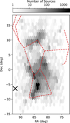 |
Fig. 1 Density distribution of sources included in our data compilation throughout the OSFC. The location of Monoceros R2 region (excluded from our compilation) is marked as a black ‘X’. |
2 Data curation
We reviewed the published literature targeting OSFC with the goal of building the largest catalogue of candidates and confirmed YSOs in the region. Our definition of the OSFC field encompasses 564 square degrees that cover the box between RA 74.2 and 92 deg and Dec −14.1 and +17.6 deg. We considered YSOs explicitly listed as members of the Monoceros R2 region (at RA, Dec: 91.94825, −6.37850 deg) to be outside our scope, although some of those were still indirectly included in our compilation. The sky distribution of 27 879 collected YSOs is shown in Fig. 1. Fig. 2 presents a schematic representation of the data curation workflow further described in this section.
2.1 Data mining strategy for historical data
The last comprehensive historical literature review for the OSFC dates back to the Handbook of Star Formation Regions (Reipurth 2008a,b; Bally 2008) more than 15 years ago. However, that review did not provide a list of known YSOs in the region that could give us a head start. Hence, instead of starting from previous literature reviews, we focussed on the entire body of peer-reviewed publications targeting the region, which have been indexed by the SAO/NASA Astrophysics Data System (Kurtz et al. 2000). This exercise was carried out with the objective of identifying and data-mining publications that focussed on the identification and characterisation of YSOs in the OSFC. Given our scope of building a census of sources where either a pro-tostar or a pre-main-sequence (PMS) star is already observable, we therefore set out to cover roughly Class 0 to Class III YSOs. Although some cores and Herbig Haro (HH) objects may be collaterally included in our historical data compilation, those sources and others intimately related to the earlier stages of the star formation (e.g. starless cores, jets, globules, etc.) are beyond our scope.
At the high stellar-mass end, our compilation includes both higher mass YSOs, such as Herbig Ae/Be, as well as O-type stars, which, although no longer young within their own evolutionary path, can still serve as a youth indicator for a coeval population covering the full mass spectrum. Whenever possible, we identified and flagged massive stars inferred to be beyond their zero-age main sequence (ZAMS). More details are given in Sect. 5.2.1.
2.1.1 Identification of relevant datasets through the NASA/ADS database
The SAO/NASA Astrophysics Data System (NASA/ADS; Kurtz et al. 2000) is a digital library operated by the Smithsonian Astrophysical Observatory under a NASA grant, which aggregates bibliographic collections for astronomy and physics. We used a Python wrapper, the NASA/ADS Developer API2 (Casey et al. 2017), to query NASA/ADS for bibliographic references that targeted the OSFC. We started with a simple query for Orion to retrieve ~ 118 000 bibliographic entries. From there, we restricted our search to the Astronomy Database, excluded non-refereed entries prior to 2020, and refereed entries published before 2018, but never cited. After this initial filtering, we retrieved textual metadata (titles, abstracts, and keywords) for ~11 000 bibliographic entries.
Next, we applied a ‘bag of words’ method to process these bibliography entries. We started by merging titles, abstracts, and keywords for each bibliographic entry into a single text-based entry. We then employed natural language processing (NLP) methods to tokenise, lemmatisate, merge multi-word terms into single tokens, remove stop words, and homogenise spelling. The processed text was then scored on the basis of the occurrence of contextual tokens provided in an input vocabulary. This input vocabulary included the following terms: ‘YSO’, ‘star formation’, ‘young’, ‘EW’, ‘emission line’, ‘line profile’, ‘pre main sequence’, ‘accretion’, ‘H-alpha’, ‘T Tauri’, ‘Herbig’, ‘disc’, ‘protoplanetary’, ‘IR-excess’, and ‘protostar’, along with alternative versions of these terms, including their abbreviations, synonyms, and derived words.
A subset of ~4500 bibliographic entries was highly scored on the basis of this vocabulary. This subset was examined by a human who inspected abstracts and manuscripts, labelled entries by thematics, and ruled out bibliographic entries that were not relevant to our compilation. For example, we excluded purely theoretical studies, investigations of YSOs in other star-forming regions that employed previously published data in Orion as a comparison to their results, studies reusing previously published observational data without relevant added value quantities, publications based on purely qualitative data, studies focussed on the interstellar medium or the Orion nebula itself, and studies focussed purely on massive stars.
After this initial human-with-domain-knowledge filtering, we reduced our list to 1201 bibliographic entries with observational data deemed relevant to our data curation. Next, this bibliography was carefully read and the data and acquisition methods were summarised as possible. This process allowed us to further discard publications where: (i) the data actually provided were not relevant to the NEMESIS project; (ii) the tabulated data were not provided by authors; (iii) the data provided was redundant and introduced in another related publication, (iv) data products were limited to photometric catalogues for the OSFC field without explicit YSO identification, such as the data could be fully retrieved via cone-search using the VizieR-SED tool (see Sect. 2.4); or, finally, (v) the data were obtained several decades ago and where already included in previous data compilations in a suitable machine-readable format, hence, also redundant. This process also included the identification of relevant meta-data within the text of the papers that were worth tabulating.
This phase of our project was finalised in January 2023, although some more recent publications were later identified and manually included in the compilation. The processing of the relevant bibliography also allowed us to identify a dozen other scientific papers that included relevant data for young stars in Orion, but did not mention the higher-level keyword ‘Orion’ in their title, abstract, or keyword list (i.e. they had not been identified by our first query with NASA/ADS).
2.1.2 Data retrieval
From the 2000s onwards, a growing number of authors made data associated with their peer-reviewed publications at least partially available at CDS via the VizieR catalogue service (here-after VizieR3; Ochsenbein et al. 2000), making data collation very straightforward once the relevant references and tables were identified. However, the data relevant to this compilation were often absent or only partially uploaded to CDS. Therefore, we further employed one or more of the six strategies detailed below to extract data from scientific publications. These are briefly described in order of efficiency (and priority).
Data were available via VizieR, or could be retrieved with widely used tools under table access protocol (TAP; Dowler et al. 2019), for example using Astronomical Data Query Language (ADQL; Osuna et al. 2008), Tool for Operations on Catalogues And Tables (TOPCAT; Taylor 2005), or astroquery (Ginsburg et al. 2019).
The table was available in electronic format at the publisher’s website in some standard data format (csv, ascii, tbl, etc.).
Tables were only available as displayed on the publisher’s website in HTML or LATEX format. TableConvert (v 2.4.2)4 tools were used to convert them to a suitable machine-readable format.
Tables were only available as published, as part of a text-based pdf file. The Tabula Tool5 (v. 1.2.1, Aristarán et al.).
Tables were only available as part of an image-based pdf (common for older publications) or as an image format within the publication. In these cases, a png or jpeg image of the table was inputted to a free optical character recognition (OCR) tool (typically OnlineOCR)6. However, we noticed that OCR tools available to us at the time were prone to imprecision affecting decimal numbers and symbols such as ‘+’ and ‘−’ Hence, this method required a careful visual comparison between the input image table and the output ASCII table to correct for imprecisions.
Relevant data were not available in tabular format and had to be interpreted and retrieved from the publication’s text.
Table C.1 summarises the methods for data retrieval employed in each of the 217 scientific publications with data collated into the NEMESIS YSO catalogue for the OSFC.
2.1.3 Data integration
We processed the data included in the historical compilation to build a master catalogue in which each YSO-candidate previously identified in the literature is attributed a unique identifier. Section 3 provides more details of this processing. For each new literature reference integrated into our compilation, the new data set was matched to the master catalogue preferentially based on the identifier codes defined in previous studies. When unique identifiers were unavailable, we employed TOP-CAT’s Pair-Match to join tables based on coordinate matching in the FK5 system. We used a 2″ matching radius as the default. After testing different radii to match publications sharing common identifier codes, this was most often the best one. However, in cases where the source publication explicitly described larger PSF or astrometric precision, a larger radius of up to 10″ was required. At each step, unmatched sources were added as new sources and received appropriate indexing. Our unique identifier, namely NEMESIS_ID, follows integer numbers from 1 to 27 915.
2.2 Data from large photometric surveys
In addition to the compilation of YSO candidates, we also built a reference photometric database for the OSFC field based on a list of large-scale photometric surveys, including observations at 34 photometric bands and covering the wavelength range 0.15–160 µm. This allowed us to build a regular baseline for our panchromatic compilation, helping us to understand our historical compilation’s detection limits and completeness. Furthermore, by retrieving data directly from these surveys’ archives and following their user documentation, we could guarantee that the catalogues were properly cleaned before they were integrated into our database. It also helped verify the reliability of the data retrieved using the VizieR-SED tool (Sect. 2.4). Unless stated otherwise, we used a 2″ matching radius to identify counterparts in our catalogue.
GALEX DR6+7: The Galaxy Evolution Explorer (GALEX) provides UV data in two bands, in the far-UV (0.15 µm) and near-UV (0.2 µm). We retrieved data for DR6+7 (Bianchi et al. 2017) through VizieR, cleaned them to remove sources contaminated with artefacts.
Pan-STARRS1 DR2: Data from the Panoramic Survey Telescope and Rapid Response System DR2 (Pan-STARRS; Chambers et al. 2017) was retrieved through the PS1 CasJobs7 SQL Server. Pan-STARRS1 covers most of the sky above declination −30o in the bands gPS1 (0.48 µm), rPS1 (0.62 µm), iPS1 (0.75 µm), ZPS1(0.87 µm), and yPS1 (0.96 µm). We retrieved aperture photometric data from the stacked version of the survey and cleaned the dataset as recommended in Flewelling et al. (2020) to remove sources of poor quality, suspected duplicates, and keep only the best quality detections.
Gaia DR3: Gaia provides all-sky photometry in the bands GG (0.50 µm), GBP (0.59 µm), GRP (0.77 µm). We retrieved both photometric and astrometric data for the OSFC field through the Gaia ESA Archive8. We followed the recommendations in the Gaia DR3 release papers and employed the C* metrics defined by Riello et al. (2021) to correct for inconsistency between different passbands. Then, as recommended by Riello et al. (2021) and Fabricius et al. (2021), we limit the effects of brightness excess towards the fainter end of the GBP passband by limiting our dataset to stars brighter than GBP = 20.9 mag. Finally, we applied the saturation corrections proposed in Appendix C.1 of Riello et al. (2021) for the brightest stars.
2MASS PSC: Data from the Two Micron All Sky Survey (2MASS; Skrutskie et al. 2006) Point Source Catalogue (PSC label) is available all-sky and were retrieved via the NASA/IPAC Infrared Science Archive (IRSA)9.
2MASS/PSC provides photometry for the NIR bands J2M (1.24 µm), H2M (1.66 µm), and Ks,2M (2.16 µm). We used the 2MASS photometric quality flag (ph_qual) to clean up the catalogue. Only sources with quality A, B, or C were kept in the main catalogue. Low-S/N sources (ph_qual=D) and upper limit detections (ph_qual=U) are kept, but as limit values.
UKIDSS DR9: Data from the United Kingdom Infrared Telescope (UKIRT) Infrared Deep Sky Survey (UKIDSS; Lawrence et al. 2007) DR9 were available for part of the OSFC as part of the Galactic Clusters Survey (GCS) and were retrieved through VizieR. The survey includes the IR bands: ZU(0.88 µm), YU (1.03 µm), JU (1.25 µm), HU (1.63 µm), and KU (2.20 µm). We cleaned the catalogue for duplicates, sources flagged as probable noise.
UHS DR2: The UKIRT Hemisphere Survey (UHS; Dye et al. 2018) covered most of the northern part of the OSFC in the JU and KU bands. We retrieved the data available from DR2 (Bruursema et al. 2023) through the WFCAM Science Archive10 ADQL service. We cleaned the catalogue for duplicates, sources flagged as saturated or probable noise.
VHS DR5: The Vista Hemisphere Survey (VHS; McMahon et al. 2013) covered the southern part of the OSFC in the YV (1.02 µm), JV (1.25 µm), and Ks,V (2.14 µm) bands. We retrieved data from DR5 through VizieR and cleaned for duplicates, sources flagged as probable noise.
WISE: The Wide-field Infrared Survey Explorer (WISE; Wright et al. 2010) observed the whole sky in four mid-IR bands: W1 (3.4 µm), W2 (4.6 µm), W3 (12µm), and W4 (22µm). For the W1 and W2 bands, we collected data from the Cat-WISE2020 Catalogue (Marocco et al. 2021), which provides photometry extracted from co-added images produced as part of the unWISE extension (Schlafly et al. 2019) based on all available observations from WISE and NEOWISE (post-cryogenic reactivation WISE mission; Mainzer et al. 2014). For the W3 and W4 bands, no new data were acquired after the cryogenic mission, and the best data release to date is still the All-Sky Release Source Catalog (AllWISE; Wright et al. 2019). We retrieved AllWISE data directly from the survey website11. As the WISE survey was not originally designed for the specific study of YSOs, the survey’s source extraction process was not optimised for the usual sky background in star-forming regions; this is an issue that was previously acknowledged and discussed by a number of authors (e.g. Koenig & Leisawitz 2014; Marton et al. 2019). The direct use of the AllWISE catalogues for studying YSOs is thus prone to include numerous sources with spurious photometric measurements, especially in the two longer wavelengths. In Appendix A, we discuss how we built a random forest (RF) classifier trained on labelled image stamps of AllWISE W3 and W4 bands to identify and remove probable spurious detections from our catalogue.
SEIP: Data from the Spitzer-enhanced imaging products (SEIPs; SEIP 2020) were retrieved via IRSA. The SEIP Source List catalogue was downloaded and processed according to the Spitzer Enhanced Imaging Products Explanatory Supplement (2013). This data release included photometry for the four Infrared Array Camera (IRAC; Fazio et al. 2004) bands I1 (3.6 µm), I2 (4.5 µm), I3 (5.8 µm), and I4 (8.0 µm), as well as photometry for the Multiband Imaging Photometer (MIPS; Rieke et al. 2004) band at M1 (24 µm). We adopted the photometry for a 3.8″ diameter aperture. We noticed that the complete cleaning recommendations in the explanatory supplement were too restrictive, especially for regions of the OSFC with an augmented sky background typical of young star-forming regions. Therefore, we limited our cleaning steps to removing extended and saturated sources.
Herschel-PACS Point Source Catalogue 2.0: We also collected data from the Herschel-PACS Point Source Catalogue 2.0 (Marton et al. 2024a), which recently employed a hybrid strategy that combined classical source detection and machine learning techniques to provide an enhanced version of the Herschel/PACS Point Source Catalogue with much higher completeness levels than previous versions. This catalogue provides data in the three PACS bands P1 (70 µm), P2 (100 µm), and P3 (160 µm). For this specific survey, we employed a 3″ matching radius.
2.3 Data from large spectroscopic surveys
We further complemented our catalogue with stellar parameters derived as part of a series of large-scale spectroscopic surveys, briefly summarised below.
Gaia DR3: Gaia DR3 includes spectroscopic data products based on low-resolution spectra from the blue and red photometers (BP/RP spectra R ~ 30–100; Andrae et al. 2023; De Angeli et al. 2023) and medium resolution spectra from the Radial Velocity Spectrometer (RVS; R ~ 11 500; Recio-Blanco et al. 2023). Along with a series of stellar parameters, the former includes the Hα emission line (Sect. 3.6) with pseudo-EWs estimated as part of the Extended Stellar Parametrizer for Emission-Line Stars (ESP-ELS; Creevey et al. 2023), and the latter includes the Ca II IR triplet (Lanzafame et al. 2023).
RAVE DR6: The Radial Velocity Experiment (RAVE; Steinmetz et al. 2020) observed medium-resolution spectra (R ~ 7500) covering the Ca-triplet region. Its Data Release 6 provides stellar parameters (log ɡ, Teff, metallicity and radial velocity) for 21 sources in our catalogue.
LAMOST DR10: The General Survey of the Large Sky Area Multi-Object Spectroscopic Telescope (LAMOST; Zhao et al. 2012) has been spectroscopically surveying half of the sky with low- (LRS: R ~ 1800) and medium- (MRS: R ~ 7500) resolution spectra. In its current public release, DR10, LAMOST data products relevant to our compilation in four of its released catalogues (LRS_stellar, LRS_astellar, LRS_mstellar, and MRS_stellar). We downloaded the v2.0 of these DR10 catalogues directly from LAMOST DR10 official webpage12. This included LAMOST-derived parameters for 5180 sources in our catalogue. GALAH DR4: The recent Galactic Archaeology with HER-MES Survey Data Release 4 (GALAH DR4; Buder et al. 2025) included parameters ([Fe/H], radial velocity, log ɡ, Teff, υ sin i, EWs for Hβ, Hα, and Li) from high-resolution spectroscopy (R ~ 28 500) for 2058 sources in our catalogue. Gaia-ESO Survey DR5: The Gaia-ESO Survey (Gilmore et al. 2022; Randich et al. 2022) DR5 5.1 Catalogue (Hourihane et al. 2023) provides stellar parameters and a series of emission lines derived from spectra observed with ESO’s UVES and GIRAFFE instruments and includes data for 741 sources in our compilation.
APOGEE DR17: Although results from a dedicated sub-survey of APOGEE in Orion are included in our historical compilation (Cottle et al. 2018), we further complemented our catalogue with stellar parameters derived with their ASP-CAP pipeline in the context of APOGEE DR17 (Abdurro’uf et al. 2022), including stellar parameters for 9429 sources in our compilation.
ASCC-2.5 V3: The third version of All-sky Compiled Catalogue of 2.5 million stars (Kharchenko 2001) provides a large compilation of spectral types for bright stars and includes spectral types for 1069 sources in our catalogue.
2.4 VizieR photometry viewer
We further complemented our database with photometric data collected using the VizieR Photometry viewer (VizieR-SED)13. Powered by CDS, VizieR-SED is a tool intended for the visualisation of photometry around a given sky position. Hence, for an input coordinate or source name, it returns photometric observations ‘extracted around a sky position from photometry-enabled catalogues in VizieR-SED, where this photometry data can be exported in typical flux density units. The interpretation of the tool’s output as an SED comes with the caution that CDS provides no guarantee that all photometry points will correspond to the target, especially in cases of extended sources VizieR-SED14. Nevertheless, VizieR-SED provides a powerful tool for data mining the CDS database, which we employed to further search for relevant archival photometry for our sources. For that purpose, we followed their API’s recommendation to develop a Python script to query VizieR around the coordinates of each of our YSO candidates. We initially used a search radius of 5″. This wider search radius was chosen purposely, as it is prone to including contaminants from neighbouring sources, and we took advantage of this to flag sources likely susceptible to such contamination (see Sect. 4.3).
For the specific purpose of complementing the SEDs of sources in our catalogue (Sect. 3.2), we reduced this radius to 2″ to minimise contamination by neighbouring sources. We visually inspected a large number of SEDs produced with VizieR-SED data and compared them with SEDs built using photometry from our historical compilation (Sect. 2.1) and large photometric surveys (Sect. 2.2), which had their magnitude-flux conversions carefully carried out by ourselves using metadata available in their original publication. This procedure allowed us to identify and exclude from the SEDs data from surveys showing large systematics compared to the larger body of data available. We post-processed VizieR-SED outputs to remove data coming from all CDS tables already included in the compilation (i.e. see Sects. 2.1 and 2.2).
We also noticed large spreads in flux density in the SEDs generated by VizieR-SED, especially in the optical range 0.4–0.8 µm. By further inspecting these data original tables, we verified that although a fraction of the spread remained unexplained, most of these could be traced back to either multi epoch surveys (YSOs are typically photometric variables as discussed in Sect. 3.8) or to surveys targeting extended sources and publishing photometry extracted for different aperture sizes (e.g. SDSS). Finally, we opted to avoid this wavelength range and kept only data in the ranges 0.1–0.4 µm and 0.8–1000 µm, which seemed less affected by these issues.
We also identified a significant number of duplicated data, introduced by scientific publications re-reporting photometric data from large surveys. For example, although we removed all 2MASS official data release tables (as this data was already included in our compilation in Sect. 2.2) many sources had VizieR SEDs with dozens of 2MASS JHKs data points, most of which had the same flux values but originated from different CDS tables. Together with multi-epoch data, this type of duplicate is problematic for quantities derived from SED-fits, as in the added-value quantities discussed in Sect. 3.3, as it biases the fit results towards the filters with a larger number of photometric points. Thus, we further processed the SEDs from VizieR-SED to aggregate photometric measurements reported under the same filter name by averaging their fluxes weighted by their uncertainties and propagating these uncertainties accordingly.
3 Criteria for inclusion in this compilation and description of historical data types
Throughout our historical data curation (Sect. 2.1), we focussed on sources in the OSFC field previously reported as young in the literature. We adopted a positive evidence rule for inclusion in the catalogue, where a given source had to be reported as a YSO candidate by at least one of the types of study discussed in this section. Our approach thus prioritises completeness over purity. In this section we summarise the main YSO identification approaches employed by the scientific publications included in our historical compilation. We note that a revision of the different criteria adopted in the literature was beyond our scope. However, we were still interested in collating data that could support the ranking sources as bona fide YSOs. Hence, in this section we also discuss a series of data types collected for this purpose. The various data types included in the catalogue are also summarised in Appendices C and D.
3.1 Colour-magnitude and Hertzsprung-Russell diagrams
Newly formed stars are still contracting gravitationally and acquiring part of their final mass from their surroundings. Because they are still larger and colder than their main sequence (MS) counterparts, YSOs are located above ZAMS when placed in colour-magnitude diagrams (CMDs) or Hertzsprung-Russell diagrams (HRDs). Our compilation includes all sources reported in the literature as candidate YSOs from CMD selections. Barrado y Navascués et al. (2004) estimate that optical-NIR CMD YSO selections based solely on photometry suffer at least ~25% contamination by field stars. This contamination level can be greatly minimised when spectroscopic constraints for stellar parameters are available, enabling reliable transposition from observed CMDs into HRDs. Although we included all CMD-selected YSO candidates in this compilation, we also collated products from spectroscopic surveys that can help address the purity of our YSO candidate list. These data products are summarised in Table D.2 and discussed in the following sections.
3.1.1 Spectral types
Our historical compilation yielded spectral types for 7485 sources. With the complementation by large surveys in Sect. 2.3, a total of 11497 sources have spectral types. We tabulated these spectral types in the MK system, with luminosity class (or peculiar spectral characteristics) provided as an extra flag when available. When multiple previous studies provided independent spectral type derivations, a list of values is reported.
3.1.2 Effective temperatures
Our compilation included 73 808 measurements of effective temperature (Teff) for 17 589 sources collated from 42 publications. These measurements have been flagged according to the method used for derivation, where: SpT-PHOT indicates Teff derivations based on standard tables of combined spectral-type and photometric data (e.g. Pecaut & Mamajek 2013); SED indicates derivations based on SED-fitting to models (e.g. Bayo et al. 2008); SPEC indicates derivations based on fitting of observed spectra to spectra libraries (Kounkel et al. 2018); PHOT indicates derivations based on fit to photometric data using Markov chain Monte Carlo (MCMC) or Bayesian methods (e.g. Da Rio et al. 2012). We did not include Teff estimations based solely on CMD placement or colour/magnitude-Teff conversions.
3.1.3 Bolometric values
The CMD YSO selection is only possible for less embedded sources that have a significant portion of their radiation already visible. For more embedded sources, a more useful parameter space is the bolometric luminosity-temperature (BLT) diagram (e.g. Chen et al. 1995). Hence, we also collected 700 derivations of bolometric temperatures (Tbol) for 381 sources derived based on SED-fitting methods in three previous studies.
3.1.4 Attributes not included
The derivation of luminosities requires knowledge of the distance to the sources and the amount of interstellar extinction in their line of sight. Luminosities estimated prior to Gaia often carry large uncertainties as a result of the uncertainties behind distance estimations. Moreover, extinction estimations are often degenerate with the Teff derivations. Thus, we opt to leave these two quantities out of our data collection because they are often biased by the type of data and methods available at the specific time of publication.
3.2 Spectral energy distributions
As part of our historical compilation, we collated photometric data covering the 0.1–1000 µm range and processed it into SEDs. When these data were provided as magnitudes, their photometric systems were identified from their publications, and magnitudes were converted into flux densities. We preferentially adopted filter profile information from the Spanish VO Filter Profile Service (SVO-FPS; Rodrigo et al. 2012; Rodrigo & Solano 2020). When photometric system information could not be recovered from the publication, the instrument web pages or official publications, we adopted generic values in the Johnson-Cousin systems. A significant number of photometric tables out there include data re-reported from previous studies. We attempted to reduce duplicates by comparing magnitudes in the same filter collected for each source down to a precision of 0.01 mag and merging duplicates. In the present version of our database, we have not included limit values. For data related to the large photometric surveys described in Sect. 2.2 we discarded data collected in the historical compilation and instead introduced our own processing of the photometry of these surveys. This greatly complemented the SEDs and guaranteed that ~94% of sources in our catalogue had at least 5 data points in their SEDs with an average of 22 data points per SED. Examples of the SEDs collected are shown in Fig. 3.
Next, we employed data obtained with the VizieR-SED tool to further complement the SEDs. As described in Sect. 2.4, these data have been post-processed to obtain averaged values. Data from this complement is also shown in Fig. 3, and this complementation helped increase the average number of data points per SED to 29, with 96% of SEDs having at least 5 data points. The typical number of points per SED and their incidence per wavelength range are illustrated in Fig. 4. A general description of the SED database is provided in Table D.3. Additionally, flags with the counts of SED data points per wavelength range are also provided and are aimed at facilitating the usage of the catalogue.
3.3 Infrared emission by circumstellar material
At the earliest phases of young stellar evolution, the dusty envelope surrounding YSOs obscures their radiation in the optical wavelengths, which is re-emitted at longer IR and radio wavelengths. Various YSO identification and characterisation methods stem from studying this re-emitted radiation. Following the seminal work of Lada (1987), one of such methods is based on the derivation of the IR spectral index, αIR, which gauges the amount of circumstellar material as the shape of the SEDs of YSOs in the IR (λ ≥ 2 µm):
 (1)
(1)
Lada (1987) initially assigned YSOs into three classes associated with the evolution of the forming stars from core collapse to a PMS phase: Class I sources were protostars still embedded in their natal material, Class II were disc-bearing PMS stars (often associated with accreting T Tauri stars), and Class III sources were PMS stars where the dusty circumstellar disc responsible for the IR-excess of YSOs has mostly dissipated. Later, Class 0 sources were included to account for the youngest deeply embedded YSOs (Andre et al. 1993), and the flat-spectrum class described sources with characteristics between Classes I and II (Greene et al. 1994). Examples of SEDs of those standard IR classes are shown in Fig. 3. With the advent of large-scale IR facilities (e.g. Spitzer. Werner et al. (2004), WISE (Wright et al. 2010), and Herschel (Pilbratt et al. 2010)), the increase and diversification of the available IR data have helped uncover physical aspects of the evolution of the YSO that could no longer be fully explained within Lada’s standard classification scheme, leading to the proposal of alternative classification schemes that include classes such as Transition discs (e.g. Hernández et al. 2007a; Luhman et al. 2008a; Fang et al. 2009; McClure et al. 2010; Dunham et al. 2014; Kim et al. 2016; Fang et al. 2013; Espaillat et al. 2014; Grant et al. 2018).
Rather than looking at SEDs, a range of IR classification schemes combines selection cuts within sets of CMDs and colour-colour diagrams into decision tree models to isolate the loci occupied by YSOs in these diagrams (Gutermuth et al. 2009; Kryukova et al. 2012; Megeath et al. 2012; Kryukova et al. 2012; Hernández et al. 2007a, 2009, 2010, 2014; Koenig et al. 2015; Cottle et al. 2018). These approaches cover the initial identification phase for a substantial portion of the YSO candidates featured in our data set. Although these techniques include cuts to exclude sources with colours and magnitudes consistent with active galactic nuclei, star-forming galaxies, sources from the asymptotic giant branch (AGB), polycyclic aromatic hydrocarbon emission and knots of shock-heated emission, contamination by these sources is expected and some of these are further addressed in Appendix E.
All sources reported by studies applying IR classification schemes to study YSOs in the OSFC field were included in our historical compilation. More details on the data types compiled are given in the next section and in Table D.4. Although we have not compiled the IR excess measurements, we included a flag pointing to bibliographic references that include these attributes.
Standard IR classification: Because a reported YSO class in any given IR classification was a criterion for including sources in this compilation, we accordingly also collected such classes as part of our historical compilation. Nevertheless, the ever-going evolution of IR classification schemes makes the collation and homogenisation of IR classes derived by different authors an impractical task. Instead, we employed the SED database described in Sect. 3.2 to homogeneously infer IR classes in the standard classification scheme. For that, we used the procedure described in Hernandez et al. (2025) to lit Eq. (1) to SEDs and derive αIR for each source using all data available within 2–24 µm. We were able to derive αIR values for 25799 sources (Fig. 5), with the requirement that at least two data points at least 2 µm apart in wavelength existed within the 2–24 µm range. For assigning IR classes, we followed the IR class definitions as employed by Großschedl et al. (2019), which is outlined in Table 1. Beyond this added value, we compiled 16 716 IR classes for 5379 sources from 30 publications. Figure 6 shows a comparison between our own αIR-index values and the 4 largest samples of αIR-index values we found in our historical compilation.
Figure 6 illustrates that data availability as a function of wavelength and methodological differences in the derivation of αIR can affect the values derived, where the spreads observed can be traced back to distinct wavelength ranges employed: 3–8 µm from Koenig et al. (2015) 2–24 µm from Großschedl et al. (2019), 3–24 µm from Megeath et al. (2012), and 3–22 µm from Getman et al. (2017), whereas Großschedl et al. (2019) shows the closest equivalence to our values by covering a range similar to ours but with different specific data available. We stress that our αIR indices were derived using all data in the wavelength range 2–24 µm as available. As we required a minimum of two data points at least 2 µm away in wavelength for αIR derivation, ~33% reported αIR values were fitted using only data in the range 2–5µm. As further discussed in Appendix B, this reduced data availability in the mid- to far-IR may result in an excess of sources misidentified as having a thin disc. To avoid such bias, we recommend using our αIR in light of the provided data availability flags. In addition to the flags for SED sampling as a function of wavelength from Sect. 3.2, in Table 1 we also provide flags with the maximum and minimum wavelength available for αIR derivation.
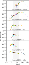 |
Fig. 3 Examples of SEDs from our database for different types of YSOs From top to bottom: a Class 0, a Class I, a Flat-Spectrum, a Class II. a Class III, and a Herbig AeBe star. See YSO classes discussion in Sect. 3.3. Photometric data collated by us is plotted in coloured symbols, while data points retrieved by processing data from the VizieR-SED tool are plotted contoured in black. The grey area shows the wavelength range used for deriving αIR indices in Sect. 3.3. |
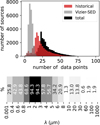 |
Fig. 4 Top: number of photometric data points in the SEDs collated into the NEMESIS YSO catalogue for the OSFC. Bottom: percentage of SEDs containing data points at a given wavelength range. |
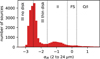 |
Fig. 5 Distribution IR spectral indices, αIR, estimated for sources in the NEMESIS Catalogue of YSOs in the OSFC using all photometric data available in the wavelength range 2–24 µm. Dotted lines show the limits between classes (Table 1). |
Standard YSO IR classes definition adopted in this study.
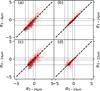 |
Fig. 6 Comparison of αIR indices derived in this study (Fig. 5) with literature values from: (a) Koenig et al. (2015), (b) Großschedl et al. (2019), (c) Megeath et al. (2012), (d) Getman et al. (2017). Dashed lines reflect a 1:1 equivalence. Dotted-black lines show the limit between YSO classes adopted in this study (Table 1). |
3.4 Lithium depletion
Lithium is quickly depleted when parts of the stellar interior reach temperatures of ~2.5 MK (Soderblom 2010). The location within the stellar interior where this takes place depends on the stellar internal structure and energy transport mechanism. In Solar-type stars, this will happen at the base of the convective zone. In the most massive fully convective stars, this takes place in their core, and in brown dwarfs below ~0.06 M⊙, the core will never get hot enough to destroy its Li (Soderblom 2010). The timescale for Li depletion is estimated between 10–50 Myr for M-type stars, 20 and a few Myr for K-type stars, but it can be much longer than YSO evolution timescales for F and G-type stars (Jeffries 2014). Nevertheless, theoretical investigations suggest that episodic accretion in young stars can produce YSOs with significantly augmented central temperatures compared to non-accreting counterparts at the same mass and age (Baraffe & Chabrier 2010). This effect can severely enhance lithium depletion in accreting YSO. Therefore, lithium detection is an excellent spectroscopic proxy for confirming the youth of YSO candidates. All sources towards the field of the OSFC identified as young through their lithium abundance evidence were included in our catalogue. Lithium observables were available as the EWs of the Li I (λ6708 Å) line or as lithium abundances, A(Li). 9185 measurements were collated from 31 publications for 6384 sources. More details on the data types collected are provided in Table D.5.
3.5 Gravity
Young stellar objects are still contracting onto the MS and have weaker surface gravity in comparison to MS stars. For comparison, while YSOs have log ɡ ~ 3–4.5, MS stars have log ɡ ~ 3.5–5, and K- and M-type giants have log ɡ ~ 1–3 (with MESA stellar evolution models as reference; Dotter 2016). Gravity observables are thus a valuable asset in distinguishing YSOs against older sources with similar spectral types. Measurements of log ɡ are typically obtained by fitting grids of synthetic spectra to observed spectra and are widely available (Da Rio et al. 2016; Kounkel et al. 2018; Yao et al. 2018; Jackson et al. 2020; Kos et al. 2021). In fact, more than 57k log g measurements were collated from 13 publications, with 12 313 sources having at least one such measurement. We note that Fig. 7 points to a degree of contamination by giants in our catalogue. This type of contamination is generally expected in surveys selecting YSOs purely from CMDs or colour-colour diagrams (as in Sect. 3.1 and Sect. 3.3). We further evaluate this contamination level in Sect. 5.2.2 and Appendix E.
Although widely available, log ɡ derivations require medium to high-resolution spectra. A cheaper alternative is the measurement of EWs of absorption lines known as surface gravity tracers (e.g. Reid et al. 1995; Slesnick et al. 2006; Schlieder et al. 2012). For example, the EWs of the Na I doublet lines are expected to be 2–3 times stronger in cool M-dwarfs than in PMS stars younger than about 10 Myr (Schiavon et al. 1997). Among many atomic and molecular bands identified as surface gravity tracers, EW observations of the lines Na I, K I, TiO, and CaH 3 have previously been reported for YSOs in the OSFC. We collated 1880 gravity-related EW measurements from nine bibliographic references, with measurements available for 1439 sources. Hence, 13 065 sources (47% of our catalogue) had gravity-related quantities collected. The general distribution of the gravity observables is shown in Fig. 7 and data types are summarised in Table D.6.
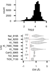 |
Fig. 7 Top: distribution of log g values collated into the NEMESIS Catalogue of YSOs in the OSFC (Sect. 3.5). Bottom: general distribution of EW values for absorption lines collected as gravity proxy. The dotted red line reflects the continuum level. Violins are shown at a fixed width for improving visualisation. Violin’s internal dotted lines reflect distributions’ first and third quartiles, and dashed lines reflect their median. |
3.6 Spectroscopic signatures of accretion and outflows
Emission lines are a defining characteristic of accreting YSOs (Joy 1945; Herbig 1962). These lines are typically formed in outflows or infalling magnetic flows, being intimately related to the accretion process (Hamann 1994; Hartigan et al. 1995; Hartmann et al. 1994; Muzerolle et al. 1998a). Extensive previous literature, including observational results and predictions from radiative transfer modelling, establishes the relationship between certain emission lines and the phenomenology behind the mass-accretion process in YSOs (e.g. Hamann & Persson 1992; Muzerolle et al. 1998b, 2001; Bouvier et al. 2007; Lima et al. 2010; Kurosawa et al. 2011; Natta et al. 2014; Alcalá et al. 2014, 2017; Wilson et al. 2022).
From an observer’s perspective, in addition to helping identify young stars, measurements of EWs of accretion-related emission lines allow us to quantify the flux in excess due to accretion, enabling estimation of mass accretion rates (e.g. Natta et al. 2004; Sacco et al. 2008; Fang et al. 2009; Alcalá et al. 2017) and help identify bona fide YSOs. With a best-effort approach, we collated a large number of measurements of relevant EWs of emission lines. Relevant spectral features are briefly discussed in this section if they were available for stars in the OSFC and included in this compilation. Although estimates of mass-accretion rates were also often available, these are heavily dependent on assumptions such as the source radius and distance, and were therefore excluded from this compilation. A summary of the EWs of collated emission lines can be found in Table D.7, and their distribution is illustrated in Fig. 8.
3.6.1 Hydrogen lines
The strongest emission line observed in the spectra of optically visible YSOs is the Hα line (e.g. White & Basri 2003). Although broad Hα is often associated with the accretion process, narrower Hα emission can also be attributed to the chromospheric activity of young stars (Martin et al. 1998). Hence, the association of Hα emission with the accretion process requires a threshold for distinction from chromospheric activity. Historically, many authors have applied thresholds with EW(Hα) at around 10 or 20 Å to identify classical T Tauri stars (CTTSs) and down to 5 Å to identify weak-line T Tauri stars (WTTSs). As the diversity of the YSOs studied spectroscopically has grown over time, spectral type-dependent classification criteria were proposed (e.g. Martin et al. 1998). Currently, the most widely used criteria are the ones of White & Basri (2003) and Barrado y Navascués & Martín (2003). However, the increasing availability of large samples of EW(Hα) seems to indicate that spectral type-dependent criteria for discerning CTTSs from WTTSs fail to identify low-accreting T Tauri stars at the end of their star-disc interaction phase (e.g. Briceño et al. 2019). This ever-going evolution of classification schemes also means that the labels for actively accreting CTTSs and non-accreting WTTSs provided in the literature depend on the classification scheme in use at the time of their publication. Therefore, we suppressed these labels from our compilation and focussed on measurements of the Hα line. Alternatively to EWs, some authors focussed on the full width at 10% of the peak of the Hα emission profile, W10%(Hα), which is proposed as an accretion diagnosis unbiased by the stellar spectral type (White & Basri 2003). Although much less widely available, we also collated these quantities. Measurements for the Hα line, whether it is EW(Hα) or W10%(Hα), are one of the most widely available spectroscopic data products, with 37 449 measurements collated from 49 publications for 21244 sources − ~76% of the sample had at least one Hα measurement.
In the absence of optical spectroscopy around the Hα line, other hydrogen lines can be used to constrain accretion. We collated 2644 EWs from 10 bibliographic references for 2501 sources, including observations for other Balmer series lines (Hβ, Hγ, and H11), lines from the Paschen series (Paβ and Paγ) and Brackett series (Brγ and Br11). Finally, the emission of molecular hydrogen, H2, is often interpreted as a signal for strong, bipolar jets or wind and can offer insight into Class 0 outflow activity (e.g. Laos et al. 2021).
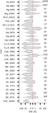 |
Fig. 8 Distribution of EWs for lines related to material inflow, out-flow and accretion in YSOs (Sect. 3.6). The dotted red line reflects the continuum level. Violins are shown at a fixed width for improving visualisation. Violin’s internal dotted lines reflect distributions’ first and third quartiles, and dashed lines reflect their median. |
3.6.2 Other lines
Beyond hydrogen lines, various emission lines in the spectra of YSOs can be traced back to the inflow and outflow of material inherent to the star-disc interaction and accretion process in these objects. He I lines are a tracer of outflow phenomena and accretion in YSOs (Kozlova et al. 1995; Sacco et al. 2008). The He I line profile is sensitive to the kinematics of the stellar wind (Connelley & Greene 2010). Hence, under certain conditions, He I can be related to chromospheric rather than accretion (e.g. Dupree et al. 1992). Nevertheless, He I has been suggested as a better tracer for identifying low-accreting stars that would otherwise be deemed non-accreting based on traditional classification schemes based solely on the emission of the Hα line (Thanathibodee et al. 2022). Ca II NIR triplet in emission is also characteristic of CTTSs (Hamann 1994; Hillenbrand et al. 1998). In the youngest YSOs, Ca II is likely produced in the pro-tostellar magnetospheric infall of gas (Muzerolle et al. 1998a) and it is considered a common emission feature for Class I YSOs (Azevedo et al. 2006; Connelley & Greene 2010), having previously been used in association with Na I and CO to distinguish them from Class II and III sources (Greene & Lada 1996). Although Ca lines in emission are often associated with accretion, these lines are instead observed in absorption for low-gravity sources (e.g. Reid et al. 1995). Finally, both forbidden lines, such as [NII], [SII], [FeII], and [OI], and some permitted lines (e.g. OI) are also often used as a tracer of outflow material (Hartigan et al. 1995; Muzerolle et al. 1998b) and have been included in the compilation when available. We collated 2849 EWs related to these processes from 16 publications for 1485 sources in our catalogue.
3.6.3 Veiling
Optical and IR veiling is also a predominant characteristic of actively creating YSOs (Herbig 1962; Basri & Bertout 1989). Veiling is thought to arise from an excess flux originating from high-temperature material in the inner disc regions, the accretion funnel, and the accretion shock regions, which is responsible for diluting the photospheric spectral lines while enhancing the spectral continuum. Veiling at a given wavelength, rλ, is typically quantified from a YSO spectrum as the ratio between the excess flux to the stellar photospheric flux (e.g. Basri & Batalha 1990; Folha & Emerson 1999). Overall, 34 358 rλ values were collected from five publications for 9588 sources. These are also summarised in Table D.7.
3.7 Kinematic methods
Due to the short timescales involved in the star formation process, observed groups of stars born from the same cloud are still moving together in relation to the galactic centre, presenting kinematic properties common to the parent cloud. Hence, groups of young coeval stars can be distinguished from foreground and background sources based on their common kinematic properties. Kinematic methods – based on variations in the star’s position in the sky – are thus widely used for selecting members of young coeval populations. There are two complementary techniques for studying stellar kinematics: the study of proper motions and the study of radial velocities. Today, reliable proper motion measurements are widely available due to Gaia, including many studies that evaluate the membership of Gaia sources in the OSFC. Members of the OSFC identified by Gaia kinematic studies are included in our catalogue if they were part of a study focussed on the OSFC or in star-forming regions (e.g. Kim et al. 2019; Zari et al. 2018). Large-scale studies typically based on machine learning, specialised in the identification of clustered populations all-sky (e.g. Hunt & Reffert 2021) were considered beyond our scope. In addition, we also collated 60 294 radial velocity measurements for 13 721 sources from 33 publications. However, two caveats must be kept in mind. First, the inclusion of kinematic members of the OSFC will include its massive population (Sect. 5.2.1). Second, radial velocities are susceptible to variations due to, for example, binarity, and these should ideally be examined in the context of an associated Julian date, which is often not reported in the studies included in our historical compilation.
3.8 Variability
Since very early studies by Joy (1945), variability has been recognised as a defining characteristic of YSOs and has since been verified across the electromagnetic spectrum (e.g. Stelzer et al. 2007; Cody et al. 2014; Rebull et al. 2015; Venuti et al. 2015; Sousa et al. 2016; Roquette et al. 2020). The OSFC has been historically pivotal in understanding the variability of YSOs (e.g. Herbst et al. 1994; Carpenter et al. 2001). Accordingly, we included YSO candidates identified in the literature based on their variability traced back to the physical phenomenology behind the evolution of YSOs.
3.8.1 Variability amplitudes
Variability amplitudes are the most widely reported variability proxy in the YSO literature. Although amplitudes have been tabulated by a number of variability studies, we note that these values are highly inhomogeneous and may be challenging to interpret as an ensemble. As an alternative, rather than collating literature values, we further added value to the catalogue by using Gaia DR3 data to added the variability degree of our sources.
Although Gaia DR3 light curves are only available for ~25% of sources in our catalogue, an alternative proxy for variability amplitude can be obtained from Gaia’s DR3 mean flux uncertainties through the AGproxy (Mowlavi et al. 2021, see their Eq. (2)), which could be calculated for 24 623 sources in our catalogue using parameters from the Gaia DR3 mean photometry.
3.8.2 Stellar rotation observables
One of the most common variability processes in YSOs is the rotational modulation by spots on the stellar surface, whether that is cool spots induced by magnetic activity or hot spots induced by accretion. Measurements of variability periods are thus often associated with YSOs spin rates (e.g. Serna et al. 2021). Due to this association, we grouped variability periods collated with υ sin i measurements in a table focussed on stellar rotation observables (i.e. Table D.10). Overall, 42 133 such observables were available for 16774 sources from 35 publications. However, we disclaim that all variability periods collected from the literature are reported in Table D.10 under the variable name Per without discerning the possible physical origins for these periods. For example, eclipsing binaries and occultation by disc material outside the co-rotation radius can also explain periodic variability in YSOs.
3.9 X-ray emission
High levels of X-ray activity are observed in YSOs at all stages of evolution from Class I to the ZAMS (Feigelson & Montmerle 1999; Preibisch et al. 2005). Additionally, since the ratio between the bolometric and X-ray luminosities for YSOs is expected to be 102–103 larger than field stars with M ~ 0.5–2 M⊙ (e.g. Feigelson & Montmerle 1999; Preibisch & Feigelson 2005; Getman et al. 2005a), X-ray observations have been established as a powerful tool for identifying YSOs. X-ray observations are especially powerful for identifying Class III, which typically lack most of the optical signatures of youth visible in Class I and II sources (e.g. Walter et al. 1988). We identified 19 publications that provided X-ray observations for 4162 likely YSOs in the OSFC. Whenever available, we collected X-ray luminosities, observed or corrected fluxes, hardness ratio, and hydrogen column density log NH. More details on the data collected are provided in Table D.11.
4 Multiplicity labels and possible duplicates
We curated labels addressing the multiplicity of sources in our catalogue in four stages: through the historical compilation (1539 sources labelled in Sect. 4.1), the use of all-sky binary catalogues from the literature (1603 sources, Sec 4.2), the use of Gaia DR3 data (6776 sources, Sect. 4.4) and derived using big data approaches (6912 sources, Sect. 4.3). As a result, 18 930 bin_type labels were assigned to 12 155 sources, which can assume the following values:
S – binary identified from spectroscopy: sources that were identified as spectroscopic binary (single or double-lined) or had observed variability in their radial velocity measurements associated with binarity.
E – eclipsing binary: sources that were reported as such in studies focussed on their light curves.
A – Astrometric binary: binaries identified based on their proper motion variations.
B – generic: sources identified as a multiple system by previous studies being re-reported in a study included in this compilation without enough accompanying information to be categorised elsewhere.
V – visual pairs: source identified as multiple from surveys with high angular resolution15.
U – unresolved pairs: Unresolved close-pairs, typically indirectly identified using Gaia data (see Sect. 4.4).
Bl – blended sources: sources likely blended with a nearby source16 (see Sect. 4.4).
R – RUWE unresolved candidate – Likely unresolved pairs identified using Gaia’s RUWE (see Sect. 4.4.3).
? – candidate: sources reported as binary candidates because the detection criteria are close to the reported significance threshold.
Figure 9 presents the relative numbers of sources in each category. Some sources have been assigned to multiple categories. For example, 28% of the sources reported as eclipsing binaries in the literature were also reported as binaries from spectroscopic investigations. We did not attempt to distinguish between binary and triple systems.
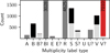 |
Fig. 9 Incidence of different multiplicity labels included in the NEME-SIS Catalogue of YSOs in the OSFC. Light grey bars show labels collected as part of the historical compilation (Sect. 4.1), black bars show labels collected from binary-focussed catalogues (Sect. 4.2), dark gray bars show labels attributed using Gaia DR3 data (Sect. 4.4), and red bars show labels attributed using big data approaches (Sect. 4.3). |
4.1 Multiplicity labels from the historical compilation
The historical data compilation described in Sect. 2.1 yielded the identification of 2006 multiplicity labels for 1539 sources (see also Fig. 9) collected from 93 publications.
4.2 Multiplicity labels from all-sky catalogues
We further searched the literature for large catalogues of binary stars that included the OSFC field and matched these to our source list. This helped us to attribute multiplicity labels to 1735 sources, 1102 of which were unlabelled in the historical compilation. This included:
(V?) 397 spatially resolved binaries with separations up to ~ 200 AU identified with Gaia eDR3 data (El-Badry et al. 2021) with low chance alignment;
(E) 11 eclipsing binaries identified in the first two years of Transiting Exoplanet Survey Satellite (TESS) observations (Prša et al. 2022);
(S) 31 double-lined spectroscopic binaries identified by Kovalev et al. (2024) using v sin i values from spectral fits to LAMOST-MRS spectra;
(S?) 460 double-lined spectroscopic binaries identified by Zheng et al. (2023) using a deep-learning approach to analyse LAMOST-MRS spectra;
(S?) 36 spectroscopic binary candidates or RV-variables identified by Qian et al. (2019) due to their large radial velocity variations in their LAMOST-LRS spectra;
(S) 19 double-lined spectroscopic binaries identified by (Traven et al. 2020) with spectra from the GALAH survey;
(S?) 2 spectroscopic binary candidates identified by Birko et al. (2019) due to their radial velocity variability in the RAVE survey;
(S?) 7 spectroscopic binary identified by Jack (2019) from a sample combining Gaia DR2 RV and RAVE spectra;
(B?) 10 ellipsoidal variable candidates selected from their TESS light-curve variability (Green et al. 2023);
(B) 615 sources from the Identification List of Binaries Catalogue, which provided a survey of surveys of literature focussing on binary stars prior to 2015 (Malkov et al. 2016);
(S) 148 sources from GALAH DR4 (Buder et al. 2025) with a secondary component detected and for which primary and radial velocity could be measured.
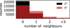 |
Fig. 10 Distribution of the number of neighbours around sources in the NEMESIS Catalogue of YSOs in the OSFC. Results for a searching radius of 2″ are shown in red, and 5″ in black. |
4.3 Big data identification of visual-pair candidates
In Sect. 2.4, we describe how we employed the VizieR-SED tool to retrieve the photometric data available on CDS around the position of each source in our catalogue. In this section we further employ these data to gauge sources’ neighbourhoods.
Starting from the raw VizieR-SED output for a 5″ searching radius, rather than relying again on the procedure described in Sect. 3.2 we carried a simpler preprocessing. We kept only data in the wavelength range 0.01–5 µm, excluding multi-epoch surveys (e.g. TESS) and surveys with source detection and extraction at different apertures (e.g. SDSS). We then grouped the remaining data by unique CDS table name and photometric band and counted how many unique pairs of RA, Dec (down to a 10−7 precision) existed. This process was repeated for each pair of CDS table name and photometric band, and the maximum number of unique sources inside the searching radius was stored as representative of the neighbourhood of that source. The same procedure was repeated using a 2″ searching radius as well. The distribution of the number of neighbours for sources in our catalogue is shown in Fig. 10.
This procedure allowed us to leverage the large amount of photometric data available from CDS to investigate the neighbourhood of sources in our catalogue, including data observed by instrumental setups yielding a wide variety of pixel scales and PSF sizes, while being agnostic to the selection window introduced by the criteria for inclusion in this compilation discussed in Sect. 3. We found that 6912 sources in our catalogue have at least one neighbour within 2" from the sources’ adopted coordinates, and 12 060 have neighbours within 5″. Sources with at least one neighbour within 2″ were labelled as visual pair candidates (V?) with the support that 71% of these sources were also identified as such by other multiplicity labels considered.
4.4 Multiplicity labels from Gaia DR3
The numerous avenues for investigating the multiplicity of sources using Gaia DR3 data merit a dedicated section.
4.4.1 Non-single source tables in Gaia DR3
We identified 223 sources with a counterpart in at least one of a series of tables focussed on non-single stars released as part of Gaia DR3 (Gaia Collaboration 2023a), which are composed of sources identified as astrometric (150 sources from nss_αccelerαtion_αstro; Halbwachs et al. 2023), spectroscopic (18 sources from nss_non_linear_spectro; Gosset et al. 2025) or eclipsing binaries (57 sources from υari_eclipsing_binary; Mowlavi et al. 2023), and with orbital models for all sources compatible with a two-body solution (ten sources from nss_two_body_orbit; Holl et al. 2023b).
4.4.2 Gaia’s scan-angle effects
Gaia’s readout window has a different size depending on the magnitude of the source and photometric band. For example, the typical window for a faint source in G is ~0.35″ × 2.1″, and ~3.5″ × 2.1″ for GBP and GRP (e.g. Riello et al. 2021; Holl et al. 2023a). In addition to this ‘rectangular’ window, to achieve full-sky coverage, Gaia has a non-trivial scanning law, including a time-varying scan-angle. While for isolated point sources, these scan-angle variations are irrelevant, for close pairs, they are determinant factors between the source being resolved or blended. For example, pairs with separations ~1″ will always be blended in BP and RP, while sources with separations ~1–2″ will occasionally be resolved when observed close to along-scan angles and can therefore be identified using Gaia’s quality control flags. Meanwhile, pairs with separations ~0.6–2″ are sometimes resolved with a six-parameter solution for the G-band (see also their Fig. 6; Lindegren et al. 2021).
Scan-angle-dependent signals: Gaia’s time-varying scan angle is hypothesised to induce scan angle-dependent signals when observing unresolved binaries or extended sources. We followed (Holl et al. 2023a) procedure to identify 191 sources likely susceptible to scan-angle biases compatible with unresolved pair numerical models (separations ≲ 1000 mas), which we labelled as U? (candidate unresolved pairs).
Scan-angle-dependent spurious variability: Gaia’s time-varying scan angle can also result in specific spurious periodic signals biasing Gaia’s epoch data. Holl et al. (2023a) and Distefano et al. (2023) attempted to identify such spurious periodicity by quantifying the correlations between Gaia’s epoch photometry and: (i) the image direction parameter determination goodness of fit (spearman_corr_ipd_ɡ_foυ), and (ii) the epoch-corrected excess factor (spearman_corr_exf_ɡ_foυ); with these parameters released as part of DR3’s table vari_spurious_signals. We identified 198 candidate unresolved sources (U?) by selecting sources with a correlation greater than 0.8 in both of these parameters.
Blended sources: Due to Gaia’s several instruments and different window sizes for the G, and the GBP and GRP bands, sources resolved in the first may be blended in the others. Gaia DR3 data processing provides flags that attempt to quantify the number of transits in which a source was blended with a nearby source. Riello et al. (2021) employs these flags to define a metric, β17, to gauge the blending fraction of source. We used this metric to flag as B1 (blended) 3028 sources that had more than 20% of their Gaia DR3 transits flagged as such (β ≥ 0.2).
4.4.3 Gaia’s re-normalised unit weight error
When observed by astrometric surveys like Gaia, stars with an unresolved or faint companion will show a different motion in their centre of light and centre of mass, which yields poor results when attempting to fit single-source astrometric models. In Gaia, such sources can be identified in terms of their re-normalised unit weight error (RUWE), which is expected to be close to one for single sources with a well-defined centre of light and uniform motion (Lindegren 2018). Since DR3, the threshold of ruwe = 1.4 (Lindegren 2018), widely used with DR2 data to distinguish between single and multiple sources, has been the subject of debate. For example, studies focussed on eclipsing binaries have found a strong correlation between RUWE values and the separations of the unresolved binaries down to ruwe = 1 (see their Fig. 3; Stassun & Torres 2021). As part of the GaiaUnlimited18, Castro-Ginard et al. (2024) provide a model to estimate suitable thresholds for binary selection with RUWE as a function of Gaia’s selection function variations as a function of sky position. This allowed us to choose appropriate RUWE values at the position of each source in our catalogue. We found an average threshold of ruwe 1.216 ± 0.038 for sources in our catalogue. GaiaUnlimited also provides tools to estimate the probability of erroneous selection of a single star with RUWE as a function of sky position, with a 5 ± 3% probability in the OSFC field. With 24 635 sources in our catalogue having at least one Gaia DR3 counterpart within 2″, and 23 716 sources having a ruwe measurement in DR3, 4625 sources were flagged ‘R’ based on our RUWE thresholds and should be interpreted as probable unresolved multiple systems.
4.4.4 Gaia’s RUWE in the context of a large sample of YSOs
As an illustrative application of our catalogue, we further contribute to probing previous suggestions that Gaia’s RUWE may be inflated in YSOs. As discussed in Sect. 4.4.3, Gaia’s astrometric solution assumes that sources are point-like with a well-defined centre of light and a single-star movement. Along with multiple systems, extended sources also deviate from these assumptions due to their non-point-like nature and the underlying larger uncertainty in resolving their centre of light. In YSOs, the diffuse emission of the envelope in Class 0/I sources, or even the radiation re-emitted by a thick disc in Class II sources, could be the culprit of an uncertain centre of light.
Considering whether the presence of a disc inflates Gaia’s RUWE: The inflation of RUWE values due to the presence of a circumstellar disc has previously been suggested by Fitton et al. (2022), based on a modest sample of 122 single stars selected from adaptative optics surveys for which they find an excess of disc-bearing sources in the RUWE range 1–2.5. Here, we contribute to probing this evidence by examining a much larger sample of YSOs. For this end, we selected sources from our catalogue with both αIR derived in Sect. 3.3, and Gaia’s DR3 RUWE.
We defined two subsamples based on αIR (Sect. 3.3), namely, sources with a thick disc (αIR ≥ −1.6) and disc-less sources (αIR ≤ −2.5). To maximise the reliability of sample selections using the αIR indices, we considered only sources with at least one data point available for λ ≥ 5 µm. We note that the requirement for Gaia data will inevitably remove the least evolved and most embedded Class I/O sources from our catalogue, as they are too faint and beyond Gaia’s detection capacity. To maximise sample purity, we also removed all sources flagged as possible contaminants in Sect. 5.2. Next, we also removed all sources flagged as multiple in Sect. 4, except for cases where the only multiplicity flag was the RUWE-based one, R (Sect. 4.4.3). This is required to preserve sources in the RUWE range that Fitton et al. (2022) claim to be populated by disc-bearing sources. Although 51% of the R labelled sample is still removed, as they were also identified as multiple systems by other methods, a modest fraction of ~10% sources with RUWE > 2.5 and likely real unresolved systems are left in the sample. To further minimise the influence of remaining binaries in our results, we focussed our analysis on the RUWE<2.5 range, which has been suggested to be the relevant range for disc-bearing sources (see Fitton et al. 2022). Our final sample was composed of 4364 disc-less sources and 1489 thick disc sources.
We employed a series of non-parametric statistical tests (Kolmogorov-Smirnov, Mann-Whitney U, and Anderson-Darling) to examine the differences between RUWE distributions of disc-bearing and disc-less sources, finding no support for significant differences between the two distributions. Alternatively, we also explored other criteria for sample selection (e.g. the use of W1 – W3 colours for thick disc selection) and other statistical approaches, such as examining disc fraction as a function of RUWE, but found no statistically significant indication of RUWE inflation due to the presence of thick discs around less evolved YSOs in our sample.
Considering whether the variability of YSOs inflates the RUWE: Beyond extended sources, photometric variability has also been proposed as a contributor to RUWE. For example, Belokurov et al. (2020) previously uncovered a trend of inflated RUWE as a function of variability amplitude for RR Lyrae and Cepheids observed with Gaia DR2. As further discussed by these authors, the inflation of RUWE by variability can be traced back to RUWE’s definition (Lindegren 2018, Eq. (4)). As its name says, RUWE is a normalised version of Gaia’s 5-parameter astrometric solution’s unit error, where a normalisation coefficient is derived from one of the modes’ unit weight error as a function of magnitude and colour. In variable stars where sharp changes of magnitude and colour take place, this normalisation may be incorrect, yielding spurious inflation of RUWE. Since variability is a prevalent characteristic of YSOs (Sect. 3.8), here we also address the influence of variability on Gaia’s DR3 RUWE.
We used Gaia DR3 AGproxy calculated in Sect. 3.8.1 (available for ~88% of the sources in our catalogue) to address the evidence for variability influence on RUWE (e.g. Belokurov et al. 2020; Barber & Mann 2023). As in the previous section, we minimised the incidence of binaries in the sample by removing all sources labelled as such, except for sources with only a R flag, and examining RUWE values up to 2.5. We also removed all sources flagged as possible contaminants in Sect. 5.2, which left us with 10 326 sources. Next, we bin the data at magnitude ranges 11 ≤ G < 13 (848 sources), 13 ≤ G < 16 (3571), 16 ≤ G < 17 (3850), and 17 ≤ G < 21: (2057) with the first two bins following Gaia’s window classes, and the remaining aimed at minimising the effects of the signal-to-noise variations with magnitude. For each magnitude bin, we estimate the first, second, and third rolling quartiles for the distributions of RUWE as functions of AGproxy. Evidence for RUWE inflation due to YSO variability is shown in Fig. 11, where variations of ≈0.03–0.18 in RUWE is seen as a function of amplitude.
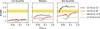 |
Fig. 11 RUWE as a function of variability amplitude (AGproxy) in Gaia DR3. A sample of YSOs (without known binaries and restricted to RUWE < 2.5) is divided into four magnitude bins, with different rolling quartiles shown in the left (first quartile), middle (median), and right (third quartile) panels. In all panels, the yellow dashed region and black-dashed line show the threshold for selection of unresolved pairs with RUWE adopted in this study. |
4.5 Possible duplicates
After extensively evaluating the multiplicity of sources in our catalogue, we are now equipped to address the incidence of duplicated sources in our data compilation process. An internal match with sources’ sky positions and a 2″radius reveals that 1864 sources are possibly duplicated. We verified that 1687 of these had a multiplicity flag derived in this section or had their possible duplication flagged as multiple. From the remaining, 119 sources could be traced back to the publications introducing them to our dataset in Sect. 2.1, which were typically surveys including higher-resolution images, and we could confirm that multiple sources were indeed reported by their original publication, 4 had support for being independent sources from a match with SIMBAD, and 20 had a neighbourhood flag (Sect. 4.3) indicative of at least one neighbour within a 5″ radius. Finally, only 34 sources could not be explained and are likely duplicates due to some coordinate mismatch in our historical data compilation. These sources were flagged accordingly.
5 Catalogue purity and contamination assessment
5.1 Comparison with SIMBAD
We used SIMBAD’s TAP service (on 13th December 2024) to retrieve data for 165 831 sources indexed by SIMBAD and located in the same field as our survey. We used a 5″ searching radius to search for possible counterparts at the position of each source in our catalogue. This relatively large searching radius was chosen to account for possible offsets between coordinates adopted in the historical compilation and the ones adopted by CDS19. We found 33 846 sources indexed by SIMBAD with a possible counterpart in our catalogue. 25 902 sources in our catalogue have at least one SIMBAD counterpart within the searching radius. All possible counterparts were recorded and are reported in our catalogue, regardless of their SIMBAD object type label (Table D.1), including 3167 sources with multiple possible counterparts. We leave it to the users of the catalogue to rank possible counterparts according to their use case.
5.1.1 Young sources known as such by SIMBAD
We followed SIMBAD User’s Guide (v1.8)20 guidelines on object types to identify 19 625 sources in the OSFC field with object_type labels indicative of T Tauri stars (TT? or TT*), YSOs (Y*?, Y*O), Ae/Be Herbig stars (Ae* or Ae?), or Orion variables (Or*, which are variable stars with irregular variability associated with eruption phenomena in young stars). We note that this list does not include objects that are arguably related to star-forming regions, such as dense cores (cor) and HH objects (HH). Although some of these sources are indirectly included in our catalogue, as discussed in Sect. 2.1, they were considered outside the main scope of our compilation. Here, we call the first group of SIMBAD’s object type labels ‘YSO labels’, i.e. labels that directly imply the source is a YSO. We call the second group ‘star-formation labels , i.e. labels that imply that the source is part of a star-forming region. Considering both sets of labels, 18 029 sources in our catalogue were already known by SIM-BAD as young. Among the 7873 sources in our catalogue with a close SIMBAD counterpart but not in the two categories of labels considered, 87% were generically labelled ‘star’ (*).
5.1.2 YSOs known by SIMBAD but missed by our compilation
Among the YSOs known by SIMBAD, 2112 were not included in our catalogue. 280 of these are located in Mon R2, which was excluded from our survey. We retrieved the bibliographic references associated with the remaining sources and verified that 1005 of them originate from studies with titles and abstracts focussed on clumps and cores, which were considered out of our scope in Sect. 2.1. 251 sources could be traced back to CDS tables included in our compilation, but were not deemed YSO candidates by the criteria in Sect. 3. The remaining sources were associated with one of the following cases. They came from all-sky variability surveys including machine-learning-generated YSO variability flags (e.g. Samus’ et al. 2017); they came from all-sky cluster membership studies with Gaia data, whereas we only included such surveys in our compilation when they were specifically tailored for studying the OSFC or star-forming regions (e.g. Zari et al. 2018); they came from studies focussed on the OSFC but did not include tables on CDS and had too few sources for their tables to make it to the list of tables digitalised by us in Sect. 2.1.2; They came from studies focussed on YSOs, but with bibliographic entries absent from the searching terms utilised in Sect. 2.1.1. Finally, we identified one bibliographic entry that adds a few dozen YSO candidates (Muench et al. 2002), which was discarded in Sect. 2.1.2 due to its focus on massive stars.
5.1.3 Sources unknown to SIMBAD
Our catalogue included 1977 sources without a counterpart in SIMBAD. It is interesting to note that although these sources were unknown to SIMBAD, 90% of them had data collected with the VizieR-SED tool within a search radius of 2″. 95% of these sources had at least 4 data points in their compiled SEDs, but some had as many as 50 data points. Beyond their SEDs, 1623 sources unknown to SIMBAD had measurements of at least one of the relevant observables discussed in Sect. 3, with 89% having αIR in Sect. 3.3 comprising 477, 847, 140, 55, and 237 were classified as disc-less class III, thin-disc class III, class II, flat-spectrum, and class 0/I, respectively. The 125 sources unknown to SIMBAD that did not include any relevant observables related to youth other than photometry could be traced back to publications included in our compilation that selected YSOs using a CMD, with 42 of these sources from Da Rio et al. (2009), 70 from Suárez et al. (2019), and 42 from Bouy et al. (2014).
5.2 Non-YSOs and catalogue purity
In Sect. 3, we employ a positive evidence rule to compose our catalogue, where a single peer-reviewed study reporting a source as a YSO candidate was enough to grant its inclusion here. We have thus prioritised the completeness of our YSO census, rather than its purity. Consequently, YSO purity must be addressed depending on the intended use of the catalogue. Although a formal evaluation of the reliability of youth indicators of each individual source in the catalogue is beyond the scope of this paper and the subject of a follow-up study, here we discuss a series of assumptions to assess our catalogue’s degree of contamination by different types of sources. To support this discussion, Fig. 12 shows a Gaia DR3 CMD for 23 716 sources in our sample with Gaia photometry and parallaxes. As a reference, we used solar-metallicity MESA isochrones (Dotter 2016).
5.2.1 Massive stars
We define massive stars as high-mass stars that are past the PMS phase. From a combination of the adopted MESA stellar evolution models with Pecaut & Mamajek (2013) Teff-spectral type scales, and considering sources at 1 Myrs, this is equivalent to sources with spectral type earlier than B3. Based on the spectral types collated in Sect. 3.1.1, 80 sources in our catalogue met this criterion (see Fig. 12 left panel), yielding a ~0.3% incidence of massive stars.
5.2.2 Contamination by giants
Because background reddened giants are a known major pollutant to YSO identification studies, we wish to further add value to our catalogue by ranking possible giant contaminants. In Sect. 3.5 we collected 57 649 loɡɡ measurements for 12 313 sources in our catalogue. Although giant contamination in our catalogue was already hinted at in Fig. 7, the direct use of these measurements for the purpose of identifying giants is hampered by the wide spread in loɡɡ derivations from different surveys. Thus, we used loɡɡ uncertainties as a statistical weight when combining multiple literature values and restricted our analysis to 6895 sources with either a 3σ dispersion or loɡɡ uncertainty (if only one measurement is available) below 0.1 dex. Figure 12 (right panel) shows the distribution of loɡɡ for this sample, which yields the identification of 537 likely giants with loɡɡ ≤ 2.5 (this threshold was chosen based on distributions of loɡɡ values in the MESA evolutionary models with the aim of minimising overlap in loɡɡ distributions of giants and YSO).
To expand the giant contamination investigation to a larger portion of our catalogue, in Appendix E we employed giants identified based on log g estimation from large spectroscopic surveys to implement a RF binary classifier trained on features from Gaia DR3 to estimate the probability that sources in our catalogue have properties comparable to a known sample of Giant stars. The results of this giant classifier for our sample are shown in the middle panel of Fig. 12. We were able to derive such probabilities for 20 546 sources in our catalogue (reported in Table D.1), and 2614 sources with high probabilities of being a Giant. We thus estimate a giant contamination level of ~13% in our catalogue. We note that among high giant probability sources, 515 sources were in the sample detected from their logg. Altogether, sources with logg indicative of giants and sources identified by our classifier correspond to 9.5% of our catalogue, suggesting a small residual incidence of unlabelled giants.
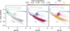 |
Fig. 12 Gaia DR3 CMD for sources in the NEMESIS Catalogue of YSOs in the OSFC (shown as black dots). Blue lines show isochrones for 1 Myr (continuous line), 10 Myr (dashed line) and 1 Gyr (dotted line). The reddening direction is indicated by the black arrow, which has an AV = 1 mag length. Left: massive stars (Sect. 5.2.1) are shown as green dots. Likely MS and post-MS contaminants in our catalogue are shown as purple dots below a 20 Myr isochrone (yellow-dashed). Middle: sources are coloured by their Giant probability derived with a RF binary classifier in Appendix E. Right: sources with log ɡ collated from spectroscopic surveys (Sect. 2.3) are shown with coloured by their log ɡ measurement (Sect. 5.2.2). |
5.2.3 Extragalact¡c contamination
As part of another study within the framework of NEMESIS (Hernandez et al. 2025), we visually identified 11 sources with galaxy morphology in photometric images. One of these sources, 2MASS J05401945-0713593 (former Internal_ID=428l) had a counterpart in the NASA/IPAC Extragalactic Database and was removed from our compilation as soon as identified. Another source, 9334 (HOPS 292), has been pointed out as a possible galaxy in the YSO literature. The other nine (4330, 4331, 4547, 4608, 4609, 7319, 7471, 7492, and 7533) are new identifications of galaxies, eight of which were previously reported as YSOs by SΓMBAD.
In Appendix E.2.1, we collate a sample of known extra-galactic sources in the field of the OSFC, including resolved and unresolved galaxies, active galactic nuclei, and quasi-stellar objects (QSOs). Among this literature-based extragalactic sample, 34 sources had a close counterpart in our catalogue. The full labelled sample was used in the implementation of a RF binary classifier trained to identify extragalactic sources based on photometric colours from the Gaia DR3, Pan-STARRs DR2, and CatWISE surveys. The trained classifier was used to evaluate the probability of 15 855 sources in our catalogue having properties comparable to the known sample of extragalactic sources. This allowed us to identify 140 likely extragalactic sources in our catalogue, 115 of which had not previously been labelled as extragalactic, yielding an estimated incidence of ~0.9% extragalactic contaminant in our sample. Figure 13 shows one of the parameter spaces defined by the features used in our classifier. Altogether, we identified 159 probable extragalactic sources in our sample (~0.6%), suggesting a small residual incidence of extragalactic contaminants.
We note that the misclassification of extragalactic sources and YSOs happens both ways. During the collation of a labelled sample for our extragalactic classifier in Appendix E, we refrained from including the Gaia DR3 QSO candidates in the labelled sample due to evidence of YSOs in this sample. Following Gaia DR3’s documentation (Gaia Collaboration 2023b) for selecting a high-purity QSO sample towards the OSFC, we found 81 QSO candidates in common with our YSO catalogue. Further examination of these sources in light of the diverse attributes included in our database revealed that a relevant fraction of such sources had compelling evidence for bona fide YSO classification in our catalogue, with 35 of these having spectroscopic constraints indicative of youth. Of the 46 remaining, 30 were identified as high probability extragalactic contaminants in Appendix E, but 16 are unaccounted. Although we opt not to include this sample in our contaminant sample, users of the catalogue who wish for a full removal of possible extragalactic sources are advised to use the extragalactic_label and strat_label (Table D.1) to identify and further inspect such sources.
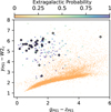 |
Fig. 13 Colour-colour diagram for the yPS1 − W2cat vs. ɡPS1 − zPS1, which are two of the features used in the Extragalactic classifier discussed in Appendix E. The colour bar reflects the derived probability of a source being likely extragalactic. Black circles show extragalactic sources reported in the literature. |
5.2.4 Further contamination
As also suggested by our comparison with SIMBAD, Fig. 12 reveals contamination by low-mass MS stars. We isolated this contamination based on a 20 Myr MESA isochrone, finding 2845 sources below the isochrone. Based on the amount of Gaia DR3 good-quality data available, this suggests a ~12.5% contamination incidence.
6 Summary of results
We assembled the largest historical compilation of YSOs in the OSFC, including 27 879 previously reported YSO candidates. The list of YSO candidates reported here included:
Young sources identified through HRD or CMD analysis or on the BLT relations of less evolved YSOs, including Teff or Tbol measurements for 63% of sources and spectral types for 41%.
Sources identified in photometric and spectroscopic studies focussed on IR emission of circumstellar material, including IR classification for 35% of sources.
Overall, 78% of sources included spectroscopic features associated with the star-disc-interaction and accretion processes in YSOs.
Youth-related spectral absorption lines such as lithium and certain gravity-sensitive spectral lines for 22% and 48% of sources.
Sources identified by kinematic studies focussed on the OSFC populations, including RV measurements collated for 49% of sources.
Variability amplitudes for 88%, and variability periods collated for 36% of sources.
X-ray emission traced back to YSOs, with X-ray luminosities or fluxes collated for 14% of sources.
Beyond the data collated from 217 previous publications, the catalogue presented here were also complemented with panchromatic data from both photometric and spectroscopic large-scale surveys. We further added value to our catalogue by
- 8.
compiling SEDs for all sources in the catalogue, with 96% of sources with at least five data points in their SEDs;
- 9.
homogeneously deriving αIR indices and IR classes for 93% of sources;
- 10.
extensively evaluating the multiplicity, resulting in 43% sources in the catalogue labelled as likely multiple sources (binary candidates or visual pairs).
Due to the positive evidence approach adopted for our data collection, our catalogue prioritises completeness over purity. We estimated that ~73% of the sources in our catalogue are reliable YSOs, with 0.3% of the catalogue composed of massive stars, while 13% are likely giant contaminants, ~1% are likely extragalactic contaminants, and 12.5% are likely MS contaminants. Finally, we estimated that the incidence of duplicates in this catalogue is below the 1% level. As an illustrative application of the catalogue, we added to the evidence that Gaia’s RUWE parameter (commonly used for identifying unresolved binaries) may be inflated in YSOs due to their prevalent photometric variability.
The present catalogue is already in use by our collaborators for upcoming publications related to the NEMESIS project. Hernandez et al. (2025) employed the catalogue to select a list of YSOs to investigate the morphology of YSOs using self-organising maps; Marton et al. (2024b, Marton et al., in prep.) used the catalogue as a training set for the identification of YSOs all-sky using deep learning techniques; and Mas et al. (2025) used the YSO observables collated here to validate the results concerning the variability of YSOs observed by Gaia DR3. Gezer et al. (2025) presented further YSO parameters by fitting YSOs’ SEDs with disc models. An ongoing study will further add value to the present catalogue through the ranking of bona fide YSOs (Roquette et al., in preparation).
Data availability
Data for Tables D.1 to D.12 are available at the CDS via https://cdsarc.cds.unistra.fr/viz-bin/cat/J/A+A/702/A63. The complete database curated as part of the NEMESIS Catalogue of YSOs for the OSFC can be accessed via SQL at https://www.astro.unige.ch/nemesis/ or at Zenodo (https://doi.org/1S.5281/zenodo.15984488).
Acknowledgements
We acknowledge funding from the European Union’s Horizon 2020 research and innovation program (grant agreement No. 101004141, NEMESIS). J.R. acknowledges support from the MERAC Foundation. G.M. acknowledges support from the János Bolyai Research Scholarship of the Hungarian Academy of Sciences. This research was also supported by the International Space Science Institute (ISSI) in Bern, through ISSI International Team project 521 selected in 2021, Revisiting Star Formation in the Era of Big Data (https://teams.issibern.ch/starformation/) We thank Berry Holl for helpful discussions on the use of Gaia DR3 data, Lynne Hillenbrand for exchanges about the large-scale collection of YSOs, and Sotiria Fotopoulou and Javier Acevedo Barroso for illuminating discussions on the identification of extragalactic sources. This work used Astropy (Astropy Collaboration 2013, 2018, 2022), Scikit-learn: Machine Learning in Python (Pedregosa et al. 2011), Pandas (The pandas development team 2020), Numpy (Harris et al. 2020), Natural Language Toolkit for Python (Bird et al. 2009), and Matplotlib (Hunter 2007).
Appendix A AllWISE Cleaning
The WISE mission (Wright et al. 2010) was designed to target IR-bright galaxies, brown dwarfs, and near-Earth asteroids. Hence, besides the convenience of its mid-IR full-sky coverage, WISE observations of YSOs in embedded environments are often susceptible to spurious detections, especially towards the far-IR. This issue has been previously investigated by a number of authors, and mitigation strategies based on AllWISE data release have been proposed to identify and remove affected sources (e.g. Koenig & Leisawitz 2014; Marton et al. 2016, 2019; Silverberg et al. 2018). In particular, Koenig & Leisawitz (2014, see their Eqs. 1 to 4) proposes that spurious detections can be separated by a series of cuts in terms of the signal-to-noise (w?snr) and profile fit reduced chi-squared (w?chi2) parameters in the AllWISE data release.
Here, we adopted a strategy similar to Marton et al. (2016, 2019), where we built a RF classifier to evaluate the reliability of WISE W3 and W4 detections based on AllWISE quality parameters and magnitudes. Nevertheless, we introduced two main modifications to the Marton et al. (2019) approach. First, Marton et al. (2019) evaluated the reliability of W3 and W4 photometry simultaneously. In contrast, we expected our sample to include sources that may only have one of these two bands above WISE’s detection limits; thus, we trained one RF classifier for each photometric band. Second, Marton et al. (2019) classifier was trained with a sample of labelled AllWISE cutouts, where a researcher visually inspected the presence or lack of a source in image cutouts at a given band. Our initial tests with this approach revealed that such labels were highly subject to the researcher carrying out the labelling. To remove this subjectivity, we used instead Astropy’s DAOStarFinder (Stetson 1987; Bradley et al. 2024) to search the cutout images for local density maxima and label them in case a source detection was successful. We built a training sample based on 5000 AllWISE cutout images around known YSOs in Orion. These cutouts have been obtained for each of the W3 and W4 bands through the IRSA WISE Image Service21 and cover a box of 10″ around the positions of the sources. Our DAOStarFinder approach allowed us to label 2356 and 1970 sources as true detections in the W3 and W4 bands, respectively.
Classification performance report for AllWISE classifiers.
Our RF classifiers were trained on samples of 3 800 labelled sources (with 50–50% labelled as true and false detections), using 21 features per band: AllWISE profile-fit magnitudes and their uncertainties (w?mpro, w?sigmpro), signal-to-noise (w?snr) and profile fit reduced chi-squared (w?chi2), the magnitudes and uncertainties at 8 different apertures (w?mag_# and w?sigm_#, where # refer to the 8 available apertures within AllWISE), and the ratios between magnitudes at consecutive apertures. Classification reports for both bands are given in Table A.1 and Confusion matrices are shown in Fig. A.1.
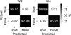 |
Fig. A.1 Confusion matrices for the training for the RF classifier for AllWISE’s W3 (left) and W4 (right). The top figure shows the confusion matrix for the W3 band, and the bottom figure shows the confusion matrix for the W4 band. |
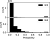 |
Fig. A.2 Distribution of reliability probability of AllWISE W3 and W4 magnitudes for sources in the field of the OSFC. |
Next, we employed the trained RF classifiers to estimate reliability probabilities for all available W3 and W4 AllWISE data in the OSFC field. This allowed us to flag 1 760 122 and 660 689 AllWISE observations in the W3 and W4 bands, respectively. The distribution of reliability probabilities for this sample is shown in Fig. A.2. For our purposes in this paper, we removed all W3 and W4 data that had probability inferior to 60%. Given the sources in our compilation with AllWISE counterparts, 17 453 (W3) and 6581 (W4) sources had reliability probability derived, out of which 10 688 (W3) and 4529 (W4) were under the threshold. Additionally, 404 (W3) and 230 (W4) sources had AllWISE counterparts in these bands but did not have all features used by the classifier available and we also eliminated these from the compilation.
Appendix B αIR reliability flags
To quantify the effect of the reduced availability of mid- to far-IR data on our αIR-indices (Sect. 3.3), we carried out an under-sampling exercise. Recalling our requirement of two data points at least 2 µm away in wavelength for αIR derivation, we selected a testing sample of 16 282 sources that followed this requirement for wavelengths λ < 5µm, and had at least one additional data point in the range 5–24 µm. For this sample, we derived an additional αIR,2–5 µm-index using only the data between 2–5 µm. Figure B.1 shows a comparison of this index to our main αIR. For the specific discussion in this appendix, we limit our αIR classes to three: disc-less, (αIR ≤ −2.5) thin disc (−2.5 < αIR < −1.6) and thick disc (αIR ≤ −2.5). We find that ~73.4% of all sources had the same class with either αIR definition (white and gray-shaded areas in Fig. B.1); ~14.8% sources were disc-less sources miss-detected as thin disc (yellow); ~8.6% were thick discs miss-detected as thin disc (green); ~1.6% were thin discs miss-detected as thick disc (red); ~1.1% of sources were thin discs miss-detected as disc-less (purple); ~0.3% were thick discs miss-detected as disc-less (blue); and ≲ 0.2% sources were disc-less miss-detected as thick discs (cyan). With 33% of our YSO candidates having no SED data points for λ ≥ 5µm, we expected such bias to affect ~9% of our αIR-indices. We note that this estimation does not take into account domain-motivated choices of the wavelength range used for αIR, and we point the interested reader to Großschedl et al. (2019) for an in-depth discussion of the effect of αIR definitions on disc classification. We also note that the numbers discussed so far refer to the total number of sources analysed. In the bottom plot of Fig. B.1, we detailed miss-classification rates normalised by the number of sources in each class derived with αIR,2–24 µm. Although only 71.2 and 66.9% of the original thick discs and disc-less sources are recovered as such, these classes have relatively large purity, with 93.7% of thick disks and 97.8% of disc-less sources correctly detected as such with the αIR,2–24 µm index. In contrast, while 88.6% of thin discs are recovered as such, this class has a much smaller purity of 74.8%.
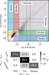 |
Fig. B.1 Comparison of αIR-indices estimated with (2–24 µm) and without (2–5 µm) illustrating the effect of mid-IR data availability into reported αIR-indices. Top: αIR,2–5 µm vs αIR,2–24 µm. Bottom: Fraction of under-sampled classification recovered as a function of disc class normalised by the number of sources in each class classified with the αIR,2–24 µm index. |
Appendix C Summary of studies included in the historical compilation
Table C.1 presents a summary of peer-reviewed scientific publications with data collated into the NEMESIS catalogue of YSOs for the OSFC.
Appendix D Database summary
The 19 thematic tables with data compiled in the present study are organised in 12 directories. A full description of directories, sub-tables, column names, units and data availability is also available as part of the online material (nemesis_osfc_description.csv). This appendix further summarises key data products, the number of individual measurements collected for each observable, and the number of sources with at least one measurement. We stress that the data is organised following a relational database paradigm. Each source is associated with a unique NEMESIS_ID key. This unique source identifier should be used to group multiple measurements (when available) for a given source and match different thematic tables.
For each quantity described in Tabs. D.1 to D.12, when available, the catalogue includes the following accompanying fields:
#: reported quantity, for example Teff for Teff or EW_Ha for EWs of the Hα line;
#_ref: NASA/ADS bibcode for the original paper linked to the reported quantity #;
e_# uncertainty;
e_up_#/e_low_# upper and lower uncertainty values;
f_# flag indicating that a limit value is reported;
#_comment: String reporting author’s comments from the original paper.
Table D.1: main/
id.csv: Complete list of sources in the NEMESIS YSO Catalogue for the OSFC, along with their reference coordinates.
contamination.csv: Contamination flags (Sects. 4.5 and 5.2).
simbad.csv: List of possible counterparts in the SIM-BAD database (Sect. 5.1).
Table D.2: hrd/ Quantities related to the HRD and BLT-diagrams (Sect. 3.1);
temperature.csv: temperatures (Sect. 3.1.2 and 3.1.3.
spt.csv Spectral types (Sect. 3.1.1).
Table D.3: sed/ SED database (Sect. 3.2)
sed_summary.csv Sumarry of data availability for SEDs
nemesis/ directory with SEDs compiled in the present study (Sect. 3.2).
vizier/ directory with SEDs compiled with the VizieR Photometry Viewer tool (Sect. 2.4).
Table D.4 ir/ : Quantities related to IR YSO classification schemes discussed Sect. 3.3;
standard_classification_nemesis.csv αIR YSO classification derived in this study.
disk_literature.csv: IR-based YSO classification collected from the literature.
Table D.5 lithium/li.csv: Lithium observables (Sect. 3.4);
Table D.6 gravity/ : gravity observables (Sect. 3.5);
ew_gravity.csv: gravity sensitive emission lines;
logg.csv: log ɡ measurements.
Table D.7: accretion/ : Quantities related to accretion or material inflow/outflow (Sect. 3.6);
ha.csv: Measurements related to the Hα line (Sect. 3.6.1);
ew_accretion_other.csv: measurement of diverse emission lines related to accretion (Sect. 3.6.2);
veiling.csv: veiling measurements (Sect. 3.6.3).
Table D.8 kinematics/rv.csv Radial velocity measurements (Sect. 3.7);
Table D.9 variability/amplitude.csv : variability amplitudes (Sect. 3.8).
Table D.10 rotation/rotation.csv: quantities related to rotation of YSOs (Sect. 3.8.2);
Table D.11: quantities related to the X-ray emission of YSOs (Sect. 3.9);
Table D.12 multiplicity/multiplicity_label.csv: Multiplicity labels (Sect. 4).
Data types in the main table.
Data types related to HRDs.
Data types related to YSOs’ IR classification.
Data types related to lithium.
Data types related to gravity.
Data types related to observables of mass inflow and outflow.
Data types likely related to radial velocity.
Data types likely related to stellar variability.
Data types likely related to stellar rotation.
Data types related to X-ray surveys.
Data types related to source multiplicity evaluation (Sect. 4).
Appendix E Extragalactic and giants contamination assessment
To investigate extragalactic and giant contamination in our catalogue, we used Scikit-learn (Pedregosa et al. 2011) to design two binary RF classifiers (Breiman 2001) trained to disaggregate these types of sources based on a set of attributes and a labelled sample. Similar classifiers specialised in the separation of stellar and extragalactic sources have been extensively implemented in the literature (e.g. Vasconcellos et al. 2011; Logan & Fotopoulou 2020; Cook et al. 2024; Lourens et al. 2024). However, these previous studies do not explicitly include YSOs in their training sample. Hence, here, we build our own classifier tailored for the OSFC field.
E.1 Data
We built a reference photometric catalogue for the OSFC field based on large photometric surveys summarised in Sect. 2.2, with a base list of 16 177 367 sources with data from Gaia DR3, Pan-STARRS1-DR2 and CatWISE. Near-infrared data were excluded because there were no surveys covering the entire OSFC field with comparable depth to the other surveys. We refer to the RF classifier trained to identify extragalactic sources against stellar sources as ‘Extragalactic classifier’, and the one trained to identify giant stars against stellar and extragalactic sources, as ‘Giant classifier’.
E.2 Labelled dataset
E.2.1 Extragalactic sources
We collated a sample of previously identified extragalactic sources, including a mixture of resolved and unresolved galaxies, active galactic nuclei, and QSOs. This accounts for 32850 sources in the OSFC field. To maximise purity, we kept only extragalactic sources with a match within 0.5″–1″ to the photo-metric reference catalogue. The list of extragalactic sources was composed of sources from:
HyperLEDA database (Makarov et al. 2014): 2638 sources;
Million Quasars catalogue v. 8 (Flesch 2023): 4641 sources;
Galaxy Zoo (Walmsley et al. 2023): 6 124 sources;
MANGROVE Catalogue (Biteau 2021): 1396 sources;
Gaia DR3 high-purity galaxy sample: 7718 sources;
Gaia DR3 high-purity QSO sample: 15 629 sources.
Extragalactic sources from Gaia DR3 were identified by Gaia’s machine learning classification and redshift estimation (Delchambre et al. 2023), brightness profile analysis (Ducourant et al. 2023), or variability behaviour (Carnerero et al. 2023; Rimoldini et al. 2023). High-purity samples were devised based on selection procedures outlined by Gaia Collaboration (2023b).
E.2.2 Stellar sources
The following samples of stellar sources were included in our labelled sample:
Certainly young: 3 698 sources from the NEMESIS YSO catalogue which have spectroscopic confirmation of youth based on significant lithium absorption in their spectra (Sect. 3.4);
At Orion’s distance: 59 146 Gaia DR3 sources with parallax consistent with a location around the location of the OSFC (300–500 pc) and parallax uncertainty better than 0.05 mas;
Giants: 13 336 sources with −0.5 ≤ log ɡ ≤ 2.5 in either RAVE, LAMOST LRS or MRS (Sect. 2.3), and log ɡ precision better than 0.25 dex;
Other Stellar Sources: 72 336 sources with log ɡ > 3.5 in either RAVE, LAMOST LRS or MRS (Sect. 2.3), and log ɡ precision better than 0.25 dex.
E.2.3 Final sample
The labelled data were further processed to remove any over-lapping labels. For example, sources labelled both certainly young and giant were removed. Further pre-cleaning of the data included removal of sources with very large uncertainties.
Extragalactic classifier sample: All sources listed in Sect. E.2.1 were initially labelled as ‘extragalactic’ (positive label), and all sources in Sect. E.2.2 were labelled as ‘stellar’ (negative label). Validation of labelled samples was carried out by comparing the locus occupied by the different samples in colour-colour diagrams. During this procedure, we verified a significant tail of ‘Gaia DR3 high-purity QSOs’ sources towards the location of stellar sources, which did not exist in the distribution of other samples with large numbers of QSOs (e.g. Million Quasars Catalogue). Furthermore, later classifier implementation tests revealed that the exclusion of ‘Gaia DR3 high-purity QSO’ labelled greatly improved the classifier recall. We therefore excluded labels from the ‘Gaia DR3 high-purity QSO’ sample from our final implementation. Further evidence that this sample suffers from contamination by YSOs is discussed in Sect. 5.2.3. A final parent sample with 23 217 and 94248 sources labelled as extragalactic and stellar was available for the Extragalactic classifier.
Giant classifier sample: Sources in the Giants sample in Sect. E.2.2 were labelled as such (positive label), and extra-galactic sources in Sect. E.2.1 or in the ‘certainly young’ and ‘other stellar’ samples were labelled as ‘other’ (negative label). We deliberately avoid the sample at Orion’s distance as this may contain Giants with unavailable log ɡ measurements. A final parent sample with 12 988 and 133 966 sources labelled as giant and others was available for the Giant classifier.
The final labelled datasets were split into 30% training, 40% validation and 30% testing sets. We ensured samples contained a representative fraction of the different source types (e.g. resolved and unresolved galaxies) by stratifying them based on origin catalogues (Sect. E.2.1), maintaining similar source proportions from each catalogue. Similarly, each subtype of stellar sources in Sect. E.2.2 was also adequately represented.
E.3 Features
Implementation tests were carried out by training classifiers in six subsets of features, combining available colours from Gaia DR3, Pan-STARRS1-DR2, and CatWISE. We included both pure-colour subsets and versions with Gaia parallaxes and uncertainties. A summary of features used in each of our best-performing models is presented in Table E.1.
E.4 Training
Class imbalance was intentionally maintained for both classifiers, as we expect giants and extragalactic sources to be a minority of sources in the OSFC field. However, this choice led to true negative labels dominating precision and accuracy. To reduce its impact on the smaller classes (true positive labels), we prioritised the use of scores that account for the trade-off between precision and recall for model comparison and performance evaluation. Additionally, as a general rule, models with validation sample true positive recovery rate under 75% were discarded. Grid search with five-fold cross-validation was performed to optimise hyperparameters, using average precision as the reference score. Each classifier was then trained with the optimal parameters and exported.
E.5 Validation
Validation samples were used for the comparison of the performance of each classifier trained, and a series of scores (namely, accuracy, precision, recall, F1-score and Fβ(β = 2) score) was used to rank their performance. For the extragalactic classifier, we found that sets of attributes covering colours from optical to mid-IR (GaiaPS1WISE_pure_colour) performed better, qualitatively consistent with results in previously published classifiers. For the giant classifier, the models using Gaia parallax performed better, with the Gaia model (attributes: Gaia colours plus parallax and its uncertainties) being only marginally outper-formed by the GaiaWISE model (same Gaia attributes with the addition of CatWISE-based colours). Nevertheless, the requirement for both Gaia and CatWISE data for the latter makes it applicable to a smaller number of sources. We therefore opt to keep the results for the pure-Gaia model (Table E.1).
Validation samples were also used to study the precision-recall curves of the best-performing classifiers. At this stage, we used the F1-score for determining the best classification thresholds while ensuring a good trade-off between precision and recall. Best classification thresholds were found at 0.41 for the extragalactic classifier, and at 0.39 for the giant classifier.
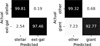 |
Fig. E.1 Confusion matrices for the extragalactic (Left) and giant (Right) RF classifiers normalised over true labels. |
E.6 Classification
We used the classification thresholds from the previous section for classification. Classification reports for the testing set are presented in Table E.2, and confusion matrices in Fig. E.1.
Extragalactic classifier: We were able to apply the GaiaPS1WISE_pure_colour model to classify 6 520 467 sources, with 139 668 classified as probable extragalactic sources. We note that among stellar sources misclassified as extragalactic (0.19 false negative rate), ~35% were spectroscopically confirmed YSOs, although these correspond to only ~3% of the YSOs in the testing sample.
Giant Classifier: We were able to apply the Gaia model to derive the probabilities of being a giant for 8 385 766 sources in the field of the OSFC, with 141 808 likely giants identified. Among sources misclassified as giants in the testing sample, 97% were labelled “other stellar sources“ based on their log ɡ measurements from spectroscopic surveys. The remaining 3% were real YSOs with spectroscopic constraints, these correspond to ~0.6% of the YSO sources in the testing sample.
The development of these classifiers included 53 154 labelled sources without enough data for classification. Both samples of classified and labelled but not classified sources were matched to the OSFC YSO catalogue and further discussed in Sect. 5.2.
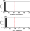 |
Fig. E.2 Distribution of probabilities of sources in the field of the OSFC being extragalactic (top) and giants (bottom). The red dotted line shows the threshold for classification. |
Features and average-precision score for the best-performing RF classifiers used for extragalactic and giant contamination evaluation.
Classification performance report of the RF extragalactic (top) and giant (bottom) classifiers.
References
- Abdurro’uf, Accetta, K., Aerts, C., et al. 2022, ApJS, 259, 35 [NASA ADS] [CrossRef] [Google Scholar]
- Abt, H. A., Wang, R., & Cardona, O. 1991, ApJ, 367, 155 [NASA ADS] [CrossRef] [Google Scholar]
- Alcalá, J. M., Covino, E., Torres, G., et al. 2000, A&A, 353, 186 [Google Scholar]
- Alcalá, J. M., Wachter, S., Covino, E., et al. 2004, A&A, 416, 677 [NASA ADS] [CrossRef] [EDP Sciences] [Google Scholar]
- Alcalá, J. M., Natta, A., Manara, C. F., et al. 2014, A&A, 561, A2 [NASA ADS] [CrossRef] [EDP Sciences] [Google Scholar]
- Alcalá, J. M., Manara, C. F., Natta, A., et al. 2017, A&A, 600, A20 [NASA ADS] [CrossRef] [EDP Sciences] [Google Scholar]
- Alecian, E., Wade, G. A., Catala, C., et al. 2009, MNRAS, 400, 354 [CrossRef] [Google Scholar]
- Ali, B., & Noriega-Crespo, A. 2004, ApJ, 613, 374 [Google Scholar]
- Andrae, R., Fouesneau, M., Sordo, R., et al. 2023, A&A, 674, A27 [CrossRef] [EDP Sciences] [Google Scholar]
- Andre, P., Ward-Thompson, D., & Barsony, M. 1993, ApJ, 406, 122 [NASA ADS] [CrossRef] [Google Scholar]
- Arun, R., Mathew, B., Rengaswamy, S., et al. 2021, MNRAS, 501, 1243 [Google Scholar]
- Astropy Collaboration (Robitaille, T. P., et al.) 2013, A&A, 558, A33 [NASA ADS] [CrossRef] [EDP Sciences] [Google Scholar]
- Astropy Collaboration (Price-Whelan, A. M., et al.) 2018, AJ, 156, 123 [Google Scholar]
- Astropy Collaboration (Price-Whelan, A. M., et al.) 2022, ApJ, 935, 167 [NASA ADS] [CrossRef] [Google Scholar]
- Azevedo, R., Calvet, N., Hartmann, L., et al. 2006, A&A, 456, 225 [NASA ADS] [CrossRef] [EDP Sciences] [Google Scholar]
- Baines, D., Oudmaijer, R. D., Mora, A., et al. 2004, MNRAS, 353, 697 [NASA ADS] [CrossRef] [Google Scholar]
- Baldovin-Saavedra, C., Audard, M., Duchêne, G., et al. 2009, ApJ, 697, 493 [Google Scholar]
- Bally, J. 2008, in Handbook of Star Forming Regions, Volume I, 4, ed. B. Reipurth, 459 [Google Scholar]
- Baraffe, I., & Chabrier, G. 2010, A&A, 521, A44 [NASA ADS] [CrossRef] [EDP Sciences] [Google Scholar]
- Barber, M. G., & Mann, A. W. 2023, ApJ, 953, 127 [NASA ADS] [CrossRef] [Google Scholar]
- Barrado, D., Stelzer, B., Morales-Calderón, M., et al. 2011, A&A, 526, A21 [NASA ADS] [CrossRef] [EDP Sciences] [Google Scholar]
- Barrado y Navascués, D., & Martin, E. L. 2003, AJ, 126, 2997 [Google Scholar]
- Barrado y Navascués, D., Stauffer, J. R., Bouvier, J., Jayawardhana, R., & Cuillandre, J.-C. 2004, ApJ, 610, 1064 [Google Scholar]
- Barrado Y Navascués, D., Bayo, A., Morales-Calderón, M., et al. 2007, A&A, 468, L5 [Google Scholar]
- Barrado y Navascués, D., Stauffer, J. R., Morales-Calderón, M., et al. 2007, ApJ, 664, 481 [CrossRef] [Google Scholar]
- Basri, G., & Batalha, C. 1990, ApJ, 363, 654 [Google Scholar]
- Basri, G., & Bertout, C. 1989, ApJ, 341, 340 [NASA ADS] [CrossRef] [Google Scholar]
- Bayo, A., Rodrigo, C., Barrado Y Navascués, D., et al. 2008, A&A, 492, 277 [NASA ADS] [CrossRef] [EDP Sciences] [Google Scholar]
- Bayo, A., Barrado, D., Stauffer, J., et al. 2011, A&A, 536, A63 [NASA ADS] [CrossRef] [EDP Sciences] [Google Scholar]
- Bayo, A., Barrado, D., Huélamo, N., et al. 2012, A&A, 547, A80 [NASA ADS] [CrossRef] [EDP Sciences] [Google Scholar]
- Béjar, V. J. S., Martin, E. L., Zapatero Osorio, M. R., et al. 2001, ApJ, 556, 830 [CrossRef] [Google Scholar]
- Béjar, V. J. S., Zapatero Osorio, M. R., Rebolo, R., et al. 2011, ApJ, 743, 64 [Google Scholar]
- Belokurov, V., Penoyre, Z., Oh, S., et al. 2020, MNRAS, 496, 1922 [Google Scholar]
- Bianchi, L., Shiao, B., & Thilker, D. 2017, ApJS, 230, 24 [Google Scholar]
- Biazzo, K., Melo, C. H. F., Pasquini, L., et al. 2009, A&A, 508, 1301 [NASA ADS] [CrossRef] [EDP Sciences] [Google Scholar]
- Bird, S., Klein, E., & Loper, E. 2009, Natural Language Processing with Python: Analyzing Text with the Natural Language Toolkit (O’Reilly Media) [Google Scholar]
- Birko, D., Zwitter, T., Grebel, E. K., et al. 2019, AJ, 158, 155 [NASA ADS] [CrossRef] [Google Scholar]
- Biteau, J. 2021, ApJS, 256, 15 [Google Scholar]
- Bolton, C. T., Harmanec, P., Lyons, R. W., Odell, A. P., & Pyper, D. M. 1998, A&A, 337, 183 [NASA ADS] [Google Scholar]
- Bossi, M., Gaspani, A., Scardia, M., & Tadini, M. 1989, A&A, 222, 117 [NASA ADS] [Google Scholar]
- Bouma, L. G., Winn, J. N., Ricker, G. R., et al. 2020, AJ, 160, 86 [NASA ADS] [CrossRef] [Google Scholar]
- Bouvier, J., Alencar, S. H. P., Harries, T. J., Johns-Krull, C. M., & Romanova, M. M. 2007, in Protostars and Planets V, eds. B. Reipurth, D. Jewitt, & K. Keil, 479 [Google Scholar]
- Bouy, H., Alves, J., Bertin, E., Sarro, L. M., & Barrado, D. 2014, A&A, 564, A29 [NASA ADS] [CrossRef] [EDP Sciences] [Google Scholar]
- Bradley, L., Sipocz, B., Robitaille, T., et al. 2024, https://doi.org/18.5281/zenodo.12585239 [Google Scholar]
- Breiman, L. 2001, Mach. Learn., 45, 5 [Google Scholar]
- Briceño, C., Calvet, N., Hernández, J., et al. 2005, AJ, 129, 907 [Google Scholar]
- Briceño, C., Hartmann, L., Hernández, J., et al. 2007, ApJ, 661, 1119 [Google Scholar]
- Briceño, C., Calvet, N., Hernández, J., et al. 2019, AJ, 157, 85 [CrossRef] [Google Scholar]
- Broos, P. S., Getman, K. V., Povich, M. S., et al. 2013, ApJS, 209, 32 [NASA ADS] [CrossRef] [Google Scholar]
- Bruursema, J., Vrba, F., Munn, J., et al. 2023, in American Astronomical Society Meeting Abstracts, 242, 118.08 [Google Scholar]
- Buder, S., Kos, J., Wang, X. E., et al. 2025, PASA, 42, e051 [Google Scholar]
- Burningham, B., Naylor, T., Littlefair, S. P., & Jeffries, R. D. 2005, MNRAS, 356, 1583 [Google Scholar]
- Caballero, J. A. 2007, A&A, 466, 917 [NASA ADS] [CrossRef] [EDP Sciences] [Google Scholar]
- Caballero, J. A. 2008, A&A, 478, 667 [NASA ADS] [CrossRef] [EDP Sciences] [Google Scholar]
- Caballero, J. A., & Solano, E. 2008, A&A, 485, 931 [NASA ADS] [CrossRef] [EDP Sciences] [Google Scholar]
- Caballero, J. A., Cabrera-Lavers, A., Garcia-Álvarez, D., & Pascual, S. 2012, A&A, 546, A59 [NASA ADS] [CrossRef] [EDP Sciences] [Google Scholar]
- Caballero, J. A., Novalbos, I., Tobal, T., & Miret, F. X. 2018, Astron. Nachr., 339, 60 [Google Scholar]
- Caballero, J. A., de Burgos, A., Alonso-Floriano, F. J., et al. 2019, A&A, 629, A114 [NASA ADS] [CrossRef] [EDP Sciences] [Google Scholar]
- Cao, L., Pinsonneault, M. H., Hillenbrand, L. A., & Kuhn, M. A. 2022, ApJ, 924, 84 [NASA ADS] [CrossRef] [Google Scholar]
- Cargile, P. A., Stassun, K. G., & Mathieu, R. D. 2008, ApJ, 674, 329 [Google Scholar]
- Carnerero, M. I., Raiteri, C. M., Rimoldini, L., et al. 2023, A&A, 674, A24 [NASA ADS] [CrossRef] [EDP Sciences] [Google Scholar]
- Carpenter, J. M., Hillenbrand, L. A., & Skrutskie, M. F. 2001, AJ, 121, 3160 [NASA ADS] [CrossRef] [Google Scholar]
- Casey, A., Sudilovsky, V., Barentsen, G., et al. 2017, A Python Module to Interact with NASA’s ADS that Doesn’t SuckTM, https://github.com/andycasey/ads [Google Scholar]
- Castro-Ginard, A., Penoyre, Z., Casey, A. R., et al. 2024, A&A, 688, A1 [NASA ADS] [CrossRef] [EDP Sciences] [Google Scholar]
- Chambers, K. C., et al. 2017, VizieR Online Data Catalog: The Pan-STARRS release 1 (PS1) Survey – DR1 (Chambers+, 2016), VizieR On-line Data Catalog: II/349. Originally published in: 2016arXiv161205560C; 2016 arXiv161205240M; 2016arXiv161205245W; 2016arXiv161205244M; 2016arXiv161205242M; 2016arXiv161205243F [Google Scholar]
- Chen, H., Myers, P. C., Ladd, E. F., & Wood, D. O. S. 1995, ApJ, 445, 377 [NASA ADS] [CrossRef] [Google Scholar]
- Cody, A. M., & Hillenbrand, L. A. 2010, ApJS, 191, 389 [NASA ADS] [CrossRef] [Google Scholar]
- Cody, A. M., Stauffer, J., Baglin, A., et al. 2014, AJ, 147, 82 [Google Scholar]
- Cohen, M., Wheaton, W. A., & Megeath, S. T. 2003, AJ, 126, 1090 [Google Scholar]
- Connelley, M. S., & Greene, T. P. 2010, AJ, 140, 1214 [Google Scholar]
- Cook, T. L., Bandi, B., Philipsborn, S., et al. 2024, MNRAS, 535, 2129 [Google Scholar]
- Correia, S., Duchêne, G., Reipurth, B., et al. 2013, A&A, 557, A63 [NASA ADS] [CrossRef] [EDP Sciences] [Google Scholar]
- Cottle, J. N., Covey, K. R., Suárez, G., et al. 2018, ApJS, 236, 27 [NASA ADS] [CrossRef] [Google Scholar]
- Covino, E., Catalano, S., Frasca, A., et al. 2000, A&A, 361, L49 [NASA ADS] [Google Scholar]
- Covino, E., Melo, C., Alcalá, J. M., et al. 2001, A&A, 375, 130 [NASA ADS] [CrossRef] [EDP Sciences] [Google Scholar]
- Creevey, O. L., Sordo, R., Pailler, F., et al. 2023, A&A, 674, A26 [NASA ADS] [CrossRef] [EDP Sciences] [Google Scholar]
- Da Rio, N., Robberto, M., Hillenbrand, L. A., Henning, T., & Stassun, K. G. 2012, ApJ, 748, 14 [Google Scholar]
- Da Rio, N., Robberto, M., Soderblom, D. R., et al. 2009, ApJS, 183, 261 [NASA ADS] [CrossRef] [Google Scholar]
- Da Rio, N., Robberto, M., Soderblom, D. R., et al. 2010, ApJ, 722, 1092 [NASA ADS] [CrossRef] [Google Scholar]
- Da Rio, N., Tan, J. C., Covey, K. R., et al. 2016, ApJ, 818, 59 [Google Scholar]
- Daemgen, S., Correia, S., & Petr-Gotzens, M. G. 2012, A&A, 540, A46 [NASA ADS] [CrossRef] [EDP Sciences] [Google Scholar]
- Damian, B., Jose, J., Biller, B., et al. 2023, ApJ, 951, 139 [NASA ADS] [CrossRef] [Google Scholar]
- Davies, C. L., Kreplin, A., Kluska, J., Hone, E., & Kraus, S. 2018, MNRAS, 474, 5406 [NASA ADS] [CrossRef] [Google Scholar]
- De Angeli, F., Weiler, M., Montegriffo, P., et al. 2023, A&A, 674, A2 [NASA ADS] [CrossRef] [EDP Sciences] [Google Scholar]
- De Furio, M., Reiter, M., Meyer, M. R., et al. 2019, ApJ, 886, 95 [NASA ADS] [CrossRef] [Google Scholar]
- De Furio, M., Liu, C., Meyer, M. R., et al. 2022a, ApJ, 941, 161 [Google Scholar]
- De Furio, M., Meyer, M. R., Reiter, M., et al. 2022b, ApJ, 925, 112 [Google Scholar]
- Delchambre, L., Bailer-Jones, C. A. L., Bellas-Velidis, I., et al. 2023, A&A, 674, A31 [NASA ADS] [CrossRef] [EDP Sciences] [Google Scholar]
- Distefano, E., Lanzafame, A. C., Brugaletta, E., et al. 2023, A&A, 674, A20 [NASA ADS] [CrossRef] [EDP Sciences] [Google Scholar]
- Dolan, C. J., & Mathieu, R. D. 2001, AJ, 121, 2124 [NASA ADS] [CrossRef] [Google Scholar]
- Dotter, A. 2016, ApJS, 222, 8 [Google Scholar]
- Dowler, P., Rixon, G., Tody, D., & Demleitner, M. 2019, Table Access Protocol Version 1.1, IVOA Recommendation 27 September 2019, https://www.ivoa.net/documents/TAP/28198927/REC-TAP-1.1.pdf [Google Scholar]
- Downes, J. J., Briceño, C., Mateu, C., et al. 2014, MNRAS, 444, 1793 [NASA ADS] [CrossRef] [Google Scholar]
- Downes, J. J., Román-Zúñiga, C., Ballesteros-Paredes, J., et al. 2015, MNRAS, 450, 3490 [NASA ADS] [CrossRef] [Google Scholar]
- Duchêne, G., Lacour, S., Moraux, E., Goodwin, S., & Bouvier, J. 2018, MNRAS, 478, 1825 [NASA ADS] [Google Scholar]
- Ducourant, C., Krone-Martins, A., Galluccio, L., et al. 2023, A&A, 674, A11 [NASA ADS] [CrossRef] [EDP Sciences] [Google Scholar]
- Dunham, M. M., Stutz, A. M., Allen, L. E., et al. 2014, in Protostars and Planets VI, eds. H. Beuther, R. S. Klessen, C. P. Dullemond, & T. Henning, 195 [Google Scholar]
- Dupree, A. K., Sasselov, D. D., & Lester, J. B. 1992, ApJ, 387, L85 [CrossRef] [Google Scholar]
- Dye, S., Lawrence, A., Read, M. A., et al. 2018, MNRAS, 473, 5113 [Google Scholar]
- El-Badry, K., Rix, H.-W., & Heintz, T. M. 2021, MNRAS, 506, 2269 [NASA ADS] [CrossRef] [Google Scholar]
- Espaillat, C., Muzerolle, J., Najita, J., et al. 2014, in Protostars and Planets VI, eds. H. Beuther, R. S. Klessen, C. P. Dullemond, & T. Henning, 497 [Google Scholar]
- Fabricius, C., Luri, X., Arenou, F., et al. 2021, A&A, 649, A5 [NASA ADS] [CrossRef] [EDP Sciences] [Google Scholar]
- Fang, M., van Boekel, R., Wang, W., et al. 2009, A&A, 504, 461 [NASA ADS] [CrossRef] [EDP Sciences] [Google Scholar]
- Fang, M., Kim, J. S., van Boekel, R., et al. 2013, ApJS, 207, 5 [NASA ADS] [CrossRef] [Google Scholar]
- Fang, M., Sicilia-Aguilar, A., Roccatagliata, V., et al. 2014, A&A, 570, A118 [NASA ADS] [CrossRef] [EDP Sciences] [Google Scholar]
- Fang, M., Kim, J. S., Pascucci, I., et al. 2017, AJ, 153, 188 [NASA ADS] [CrossRef] [Google Scholar]
- Fang, M., Kim, J. S., Pascucci, I., & Apai, D. 2021, ApJ, 908, 49 [NASA ADS] [CrossRef] [Google Scholar]
- Fazio, G. G., Hora, J. L., Allen, L. E., et al. 2004, ApJS, 154, 10 [Google Scholar]
- Federman, S., Megeath, S. T., Tobin, J. J., et al. 2023, ApJ, 944, 49 [NASA ADS] [CrossRef] [Google Scholar]
- Feigelson, E. D., & Montmerle, T. 1999, ARA&A, 37, 363 [Google Scholar]
- Feigelson, E. D., Broos, P., Gaffney, III, J. A., et al. 2002, ApJ, 574, 258 [NASA ADS] [CrossRef] [Google Scholar]
- Fernandez, M. A., Covey, K. R., De Lee, N., et al. 2017, PASP, 129, 084201 [NASA ADS] [CrossRef] [Google Scholar]
- Furész, G., Hartmann, L. W., Megeath, S. T., Szentgyorgyi, A. H., & Hamden, E. T. 2008, ApJ, 676, 1109 [Google Scholar]
- Fischer, W. J., Megeath, S. T., Furlan, E., et al. 2020, ApJ, 905, 119 [NASA ADS] [CrossRef] [Google Scholar]
- Fitton, S., Tofflemire, B. M., & Kraus, A. L. 2022, RNAAS, 6, 18 [NASA ADS] [Google Scholar]
- Flaccomio, E., Damiani, F., Micela, G., et al. 2003, ApJ, 582, 382 [NASA ADS] [CrossRef] [Google Scholar]
- Flaischlen, S., Preibisch, T., Kluge, M., Manara, C. F., & Ercolano, B. 2022, A&A, 666, A55 [NASA ADS] [CrossRef] [EDP Sciences] [Google Scholar]
- Flesch, E. W. 2023, Open J. Astrophys., 6, 49 [NASA ADS] [CrossRef] [Google Scholar]
- Flewelling, H. A., Magnier, E. A., Chambers, K. C., et al. 2020, ApJS, 251, 7 [NASA ADS] [CrossRef] [Google Scholar]
- Folha, D. F. M., & Emerson, J. P. 1999, A&A, 352, 517 [NASA ADS] [Google Scholar]
- Franciosini, E., & Sacco, G. G. 2011, A&A, 530, A150 [NASA ADS] [CrossRef] [EDP Sciences] [Google Scholar]
- Franciosini, E., Pallavicini, R., & Sanz-Forcada, J. 2006, A&A, 446, 501 [NASA ADS] [CrossRef] [EDP Sciences] [Google Scholar]
- Franciosini, E., Tognelli, E., Degl’Innocenti, S., et al. 2022, A&A, 659, A85 [NASA ADS] [CrossRef] [EDP Sciences] [Google Scholar]
- Frasca, A., Covino, E., Spezzi, L., et al. 2009, A&A, 508, 1313 [NASA ADS] [CrossRef] [EDP Sciences] [Google Scholar]
- Frasca, A., Boffin, H. M. J., Manara, C. F., et al. 2021, A&A, 656, A138 [NASA ADS] [CrossRef] [EDP Sciences] [Google Scholar]
- Furlan, E., Fischer, W. J., Ali, B., et al. 2016, ApJS, 224, 5 [Google Scholar]
- Gagne, M., & Caillault, J.-P. 1994, ApJ, 437, 361 [Google Scholar]
- Gaia Collaboration (Arenou, F., et al.) 2023a, A&A, 674, A34 [CrossRef] [EDP Sciences] [Google Scholar]
- Gaia Collaboration (Bailer-Jones, C. A. L., et al.) 2023b, A&A, 674, A41 [NASA ADS] [CrossRef] [EDP Sciences] [Google Scholar]
- Gaia ESA Archive, official webpage, https://gea.esac.esa.int/archive/ [Google Scholar]
- Genova, F., Egret, D., Bienaymé, O., et al. 2000, A&AS, 143, 1 [NASA ADS] [CrossRef] [EDP Sciences] [Google Scholar]
- Getman, K. V., Feigelson, E. D., Grosso, N., et al. 2005a, ApJS, 160, 353 [NASA ADS] [CrossRef] [Google Scholar]
- Getman, K. V., Flaccomio, E., Broos, P. S., et al. 2005b, ApJS, 160, 319 [NASA ADS] [CrossRef] [Google Scholar]
- Getman, K. V., Broos, P. S., Kuhn, M. A., et al. 2017, ApJS, 229, 28 [Google Scholar]
- Getman, K. V., Kuhn, M. A., Feigelson, E. D., et al. 2018, MNRAS, 477, 298 [NASA ADS] [CrossRef] [Google Scholar]
- Gezer, I., Marton, G., Roquette, J., et al. 2025, A&A, 696, A196 [NASA ADS] [CrossRef] [EDP Sciences] [Google Scholar]
- Gies, D. R., Barry, D. J., Bagnuolo, W. G., Jr., Sowers, J., & Thaller, M. L. 1996, ApJ, 469, 884 [Google Scholar]
- Gilmore, G., Randich, S., Worley, C. C., et al. 2022, A&A, 666, A120 [NASA ADS] [CrossRef] [EDP Sciences] [Google Scholar]
- Ginsburg, A., Sipocz, B. M., Brasseur, C. E., et al. 2019, AJ, 157, 98 [NASA ADS] [CrossRef] [Google Scholar]
- Gómez Maqueo Chew, Y., Stassun, K. G., Prša, A., et al. 2012, ApJ, 745, 58 [Google Scholar]
- Gosset, E., Damerdji, Y., Morel, T., et al. 2025, A&A, 693, A124 [NASA ADS] [CrossRef] [EDP Sciences] [Google Scholar]
- Grant, S. L., Espaillat, C. C., Megeath, S. T., et al. 2018, ApJ, 863, 13 [Google Scholar]
- GRAVITY Collaboration (Karl, M., et al.) 2018, A&A, 620, A116 [NASA ADS] [CrossRef] [EDP Sciences] [Google Scholar]
- Green, M. J., Maoz, D., Mazeh, T., et al. 2023, MNRAS, 522, 29 [CrossRef] [Google Scholar]
- Greene, T. P., & Lada, C. J. 1996, ApJ, 461, 345 [Google Scholar]
- Greene, T. P., Wilking, B. A., Andre, P., Young, E. T., & Lada, C. J. 1994, ApJ, 434, 614 [NASA ADS] [CrossRef] [Google Scholar]
- Grinin, V. P., Rostopchina, A. N., Barsunova, O. Y., & Demidova, T. V. 2010, Astrophysics, 53, 367 [Google Scholar]
- Großschedl, J. E., Alves, J., Teixeira, P. S., et al. 2019, A&A, 622, A149 [NASA ADS] [CrossRef] [EDP Sciences] [Google Scholar]
- Gutermuth, R. A., Megeath, S. T., Myers, P. C., et al. 2009, ApJS, 184, 18 [Google Scholar]
- Habel, N. M., Megeath, S. T., Booker, J. J., et al. 2021, ApJ, 911, 153 [NASA ADS] [CrossRef] [Google Scholar]
- Halbwachs, J.-L., Pourbaix, D., Arenou, F., et al. 2023, A&A, 674, A9 [NASA ADS] [CrossRef] [EDP Sciences] [Google Scholar]
- Hamann, F. 1994, ApJS, 93, 485 [NASA ADS] [CrossRef] [Google Scholar]
- Hamann, F., & Persson, S. E. 1992, ApJS, 82, 247 [NASA ADS] [CrossRef] [Google Scholar]
- Harris, C. R., Millman, K. J., van der Walt, S. J., et al. 2020, Nature, 585, 357 [NASA ADS] [CrossRef] [Google Scholar]
- Hartigan, P., Edwards, S., & Ghandour, L. 1995, ApJ, 452, 736 [Google Scholar]
- Hartmann, L., Hewett, R., & Calvet, N. 1994, ApJ, 426, 669 [Google Scholar]
- Hasenberger, B., Forbrich, J., Alves, J., et al. 2016, A&A, 593, A7 [EDP Sciences] [Google Scholar]
- Herbig, G. H. 1962, Adv. Astron. Astrophys., 1, 47 [Google Scholar]
- Herbig, G. H., & Griffin, R. F. 2006, AJ, 132, 1763 [Google Scholar]
- Herbst, W., Herbst, D. K., Grossman, E. J., & Weinstein, D. 1994, AJ, 108, 1906 [Google Scholar]
- Herbst, W., Rhode, K. L., Hillenbrand, L. A., & Curran, G. 2000, AJ, 119, 261 [Google Scholar]
- Herbst, W., Bailer-Jones, C. A. L., Mundt, R., Meisenheimer, K., & Wackermann, R. 2002, A&A, 396, 513 [EDP Sciences] [Google Scholar]
- Hernandez, D., Dionatos, O., Audard, M., et al. 2025, A&A, accepted, https://doi.org/18.1851/8884-6361/282453424 [Google Scholar]
- Hernández, J., Calvet, N., Briceño, C., et al. 2007a, ApJ, 671, 1784 [Google Scholar]
- Hernández, J., Hartmann, L., Megeath, T., et al. 2007b, ApJ, 662, 1067 [Google Scholar]
- Hernández, J., Calvet, N., Hartmann, L., et al. 2009, ApJ, 707, 705 [Google Scholar]
- Hernández, J., Morales-Calderon, M., Calvet, N., et al. 2010, ApJ, 722, 1226 [Google Scholar]
- Hernández, J., Calvet, N., Perez, A., et al. 2014, ApJ, 794, 36 [CrossRef] [Google Scholar]
- Hernández, J., Zamudio, L. F., Briceño, C., et al. 2023, AJ, 165, 205 [Google Scholar]
- Hesser, J. E., Walborn, N. R., & Ugarte, P. P. 1976, Nature, 262, 116 [NASA ADS] [CrossRef] [Google Scholar]
- Hillenbrand, L. A. 1997, AJ, 113, 1733 [Google Scholar]
- Hillenbrand, L. A., Strom, S. E., Calvet, N., et al. 1998, AJ, 116, 1816 [NASA ADS] [CrossRef] [Google Scholar]
- Hillenbrand, L. A., Hoffer, A. S., & Herczeg, G. J. 2013, AJ, 146, 85 [NASA ADS] [CrossRef] [Google Scholar]
- Holl, B., Fabricius, C., Portell, J., et al. 2023a, A&A, 674, A25 [NASA ADS] [CrossRef] [EDP Sciences] [Google Scholar]
- Holl, B., Sozzetti, A., Sahlmann, J., et al. 2023b, A&A, 674, A10 [NASA ADS] [CrossRef] [EDP Sciences] [Google Scholar]
- Hourihane, A., Francois, P., Worley, C. C., et al. 2023, A&A, 676, A129 [NASA ADS] [CrossRef] [EDP Sciences] [Google Scholar]
- Hsu, W.-H., Hartmann, L., Allen, L., et al. 2012, ApJ, 752, 59 [Google Scholar]
- Hsu, W.-H., Hartmann, L., Allen, L., et al. 2013, ApJ, 764, 114 [Google Scholar]
- Hunt, E. L., & Reffert, S. 2021, A&A, 646, A104 [NASA ADS] [CrossRef] [EDP Sciences] [Google Scholar]
- Hunter, J. D. 2007, Comput. Sci. Eng., 9, 90 [NASA ADS] [CrossRef] [Google Scholar]
- Ingleby, L., Calvet, N., Hernández, J., et al. 2011, AJ, 141, 127 [NASA ADS] [CrossRef] [Google Scholar]
- Ingraham, P., Albert, L., Doyon, R., & Artigau, E. 2014, ApJ, 782, 8 [Google Scholar]
- Irwin, J., Aigrain, S., Hodgkin, S., et al. 2007, MNRAS, 380, 541 [Google Scholar]
- Jack, D. 2019, Astron. Nachr., 340, 386 [Google Scholar]
- Jackson, R. J., Jeffries, R. D., Wright, N. J., et al. 2020, MNRAS, 496, 4701 [NASA ADS] [CrossRef] [Google Scholar]
- Jaehnig, K., Bird, J. C., Stassun, K. G., et al. 2017, ApJ, 851, 14 [Google Scholar]
- Jayasinghe, T., Kochanek, C. S., Stanek, K. Z., et al. 2018, MNRAS, 477, 3145 [Google Scholar]
- Jeffries, R. D. 2014, in EAS Publications Series, 65, eds. Y. Lebreton, D. Valls-Gabaud, & C. Charbonnel, 289 [NASA ADS] [CrossRef] [EDP Sciences] [Google Scholar]
- Jerabkova, T., Beccari, G., Boffin, H. M. J., et al. 2019, A&A, 627, A57 [NASA ADS] [CrossRef] [EDP Sciences] [Google Scholar]
- Joy, A. H. 1945, ApJ, 102, 168 [Google Scholar]
- Karim, T., Stassun, K. G., Briceño, C., et al. 2016, AJ, 152, 198 [NASA ADS] [CrossRef] [Google Scholar]
- Kenyon, M. J., Jeffries, R. D., Naylor, T., Oliveira, J. M., & Maxted, P. F. L. 2005, MNRAS, 356, 89 [NASA ADS] [CrossRef] [Google Scholar]
- Kharchenko, N. V. 2001, Kinemat. Fiz. Nebesnykh Tel, 17, 409 [NASA ADS] [Google Scholar]
- Kim, K. H., Watson, D. M., Manoj, P., et al. 2013, ApJ, 769, 149 [Google Scholar]
- Kim, K. H., Watson, D. M., Manoj, P., et al. 2016, ApJS, 226, 8 [Google Scholar]
- Kim, D., Lu, J. R., Konopacky, Q., et al. 2019, AJ, 157, 109 [Google Scholar]
- Koenig, X. P., & Leisawitz, D. T. 2014, ApJ, 791, 131 [Google Scholar]
- Koenig, X., Hillenbrand, L. A., Padgett, D. L., & DeFelippis, D. 2015, AJ, 150, 100 [NASA ADS] [CrossRef] [Google Scholar]
- Köhler, R., Petr-Gotzens, M. G., McCaughrean, M. J., et al. 2006, A&A, 458, 461 [Google Scholar]
- Kos, J., Bland-Hawthorn, J., Buder, S., et al. 2021, MNRAS, 506, 4232 [NASA ADS] [CrossRef] [Google Scholar]
- Kounkel, M., Hartmann, L., Tobin, J. J., et al. 2016a, ApJ, 821, 8 [Google Scholar]
- Kounkel, M., Megeath, S. T., Poteet, C. A., Fischer, W. J., & Hartmann, L. 2016b, ApJ, 821, 52 [NASA ADS] [CrossRef] [Google Scholar]
- Kounkel, M., Hartmann, L., Calvet, N., & Megeath, T. 2017a, AJ, 154, 29 [NASA ADS] [CrossRef] [Google Scholar]
- Kounkel, M., Hartmann, L., Loinard, L., et al. 2017b, ApJ, 834, 142 [Google Scholar]
- Kounkel, M., Hartmann, L., Mateo, M., & Bailey, John I., I. 2017c, ApJ, 844, 138 [NASA ADS] [CrossRef] [Google Scholar]
- Kounkel, M., Covey, K., Suárez, G., et al. 2018, AJ, 156, 84 [NASA ADS] [CrossRef] [Google Scholar]
- Kounkel, M., Covey, K., Moe, M., et al. 2019, AJ, 157, 196 [NASA ADS] [CrossRef] [Google Scholar]
- Kounkel, M., Covey, K., & Stassun, K. G. 2020, AJ, 160, 279 [NASA ADS] [CrossRef] [Google Scholar]
- Kounkel, M., Stassun, K. G., Bouma, L. G., et al. 2022, AJ, 164, 137 [NASA ADS] [CrossRef] [Google Scholar]
- Kovalev, M., Zhou, Z., Chen, X., & Han, Z. 2024, MNRAS, 527, 521 [Google Scholar]
- Kozlova, O. V., Grinin, V. P., & Rostopchina, A. N. 1995, Astron. Astrophys. Trans., 8, 249 [Google Scholar]
- Kryukova, E., Megeath, S. T., Gutermuth, R. A., et al. 2012, AJ, 144, 31 [Google Scholar]
- Kuhn, M. A., Povich, M. S., Luhman, K. L., et al. 2013, ApJS, 209, 29 [NASA ADS] [CrossRef] [Google Scholar]
- Kuhn, M. A., Feigelson, E. D., Getman, K. V., et al. 2014, ApJ, 787, 107 [Google Scholar]
- Kurosawa, R., Romanova, M. M., & Harries, T. J. 2011, MNRAS, 416, 2623 [NASA ADS] [CrossRef] [Google Scholar]
- Kurtz, M. J., Eichhorn, G., Accomazzi, A., et al. 2000, A&AS, 143, 41 [NASA ADS] [CrossRef] [EDP Sciences] [Google Scholar]
- Lada, C. J. 1987, in Star Forming Regions, 115, eds. M. Peimbert, & J. Jugaku, 1 [Google Scholar]
- Lanzafame, A. C., Brugaletta, E., Frémat, Y., et al. 2023, A&A, 674, A30 [NASA ADS] [CrossRef] [EDP Sciences] [Google Scholar]
- Laos, S., Greene, T. P., Najita, J. R., & Stassun, K. G. 2021, ApJ, 921, 110 [NASA ADS] [CrossRef] [Google Scholar]
- Lavail, A., Kochukhov, O., Hussain, G. A. J., et al. 2020, MNRAS, 497, 632 [Google Scholar]
- Lawrence, A., Warren, S. J., Almaini, O., et al. 2007, MNRAS, 379, 1599 [Google Scholar]
- Lee, H.-T., & Chen, W. P. 2007, ApJ, 657, 884 [CrossRef] [Google Scholar]
- Leone, F., Bohlender, D. A., Bolton, C. T., et al. 2010, MNRAS, 401, 2739 [NASA ADS] [CrossRef] [Google Scholar]
- Lewis, J. A., & Lada, C. J. 2016, ApJ, 825, 91 [Google Scholar]
- Lima, G. H. R. A., Alencar, S. H. P., Calvet, N., Hartmann, L., & Muzerolle, J. 2010, A&A, 522, A104 [NASA ADS] [CrossRef] [EDP Sciences] [Google Scholar]
- Lindegren, L. 2018, https://api.semanticscholar.org/CorpusID:195836829 [Google Scholar]
- Lindegren, L., Klioner, S. A., Hernández, J., et al. 2021, A&A, 649, A2 [EDP Sciences] [Google Scholar]
- Lloyd, C., & Stickland, D. J. 1999, Inform. Bull. Variable Stars, 4809, 1 [Google Scholar]
- Logan, C. H. A., & Fotopoulou, S. 2020, A&A, 633, A154 [NASA ADS] [CrossRef] [EDP Sciences] [Google Scholar]
- López-Santiago, J., & Caballero, J. A. 2008, A&A, 491, 961 [NASA ADS] [CrossRef] [EDP Sciences] [Google Scholar]
- López-Garcia, M. A., López-Santiago, J., Albacete-Colombo, J. F., Pérez-González, P. G., & de Castro, E. 2013, MNRAS, 429, 775 [CrossRef] [Google Scholar]
- Lourens, M. A. A., Trager, S. C., Kim, Y., Telea, A. C., & Roerdink, J. B. T. M. 2024, A&A, 690, A224 [NASA ADS] [CrossRef] [EDP Sciences] [Google Scholar]
- Luhman, K. L., Allen, L. E., Allen, P. R., et al. 2008a, ApJ, 675, 1375 [NASA ADS] [CrossRef] [Google Scholar]
- Luhman, K. L., Hernandez, J., Downes, J. J., Hartmann, L., & Briceño, C. 2008b, ApJ, 688, 362 [NASA ADS] [CrossRef] [Google Scholar]
- Mace, G. N., Prato, L., Wasserman, L. H., et al. 2009, AJ, 137, 3487 [Google Scholar]
- Madarász, M., Marton, G., Gezer, I., et al. 2025, A&A, 696, A37 [NASA ADS] [CrossRef] [EDP Sciences] [Google Scholar]
- Maheswar, G., Manoj, P., & Bhatt, H. C. 2003, A&A, 402, 963 [NASA ADS] [CrossRef] [EDP Sciences] [Google Scholar]
- Mainzer, A., Bauer, J., Cutri, R. M., et al. 2014, ApJ, 792, 30 [Google Scholar]
- Mairs, S., Lalchand, B., Bower, G. C., et al. 2019, ApJ, 871, 72 [Google Scholar]
- Makarov, D., Prugniel, P., Terekhova, N., Courtois, H., & Vauglin, I. 2014, A&A, 570, A13 [NASA ADS] [CrossRef] [EDP Sciences] [Google Scholar]
- Malkov, O., Karchevsky, A., Kaygorodov, P., & Kovaleva, D. 2016, Baltic Astron., 25, 49 [Google Scholar]
- Manara, C. F., Robberto, M., Da Rio, N., et al. 2012, ApJ, 755, 154 [NASA ADS] [CrossRef] [Google Scholar]
- Manset, N., & Bastien, P. 2002, AJ, 124, 1089 [Google Scholar]
- Manzo-Martínez, E., Calvet, N., Hernandez, J., et al. 2020, ApJ, 893, 56 [CrossRef] [Google Scholar]
- Marocco, F., Eisenhardt, P. R. M., Fowler, J. W., et al. 2021, ApJS, 253, 8 [Google Scholar]
- Marschall, L. A., & Mathieu, R. D. 1988, AJ, 96, 1956 [Google Scholar]
- Martin, E. L., Montmerle, T., Gregorio-Hetem, J., & Casanova, S. 1998, MNRAS, 300, 733 [Google Scholar]
- Marton, G., Tóth, L. V., Paladini, R., et al. 2016, MNRAS, 458, 3479 [Google Scholar]
- Marton, G., Ábrahám, P., Szegedi-Elek, E., et al. 2019, MNRAS, 487, 2522 [Google Scholar]
- Marton, G., Gezer, I., Madarász, M., et al. 2024a, A&A, 688, A203 [NASA ADS] [CrossRef] [EDP Sciences] [Google Scholar]
- Marton, G., Roquette, J., Madarász, M., et al. 2024b, in EAS2024, European Astronomical Society Annual Meeting, 1922 [Google Scholar]
- Mas, C., Roquette, J., Audard, M., et al. 2025, A&A, submitted [arXiv:2503.23530] [Google Scholar]
- Mathieu, R. D., Adams, F. C., & Latham, D. W. 1991, AJ, 101, 2184 [NASA ADS] [CrossRef] [Google Scholar]
- Maxted, P. F. L., Jeffries, R. D., Oliveira, J. M., Naylor, T., & Jackson, R. J. 2008, MNRAS, 385, 2210 [CrossRef] [Google Scholar]
- McBride, A., & Kounkel, M. 2019, ApJ, 884, 6 [NASA ADS] [CrossRef] [Google Scholar]
- McClure, M. K., Furlan, E., Manoj, P., et al. 2010, ApJS, 188, 75 [NASA ADS] [CrossRef] [Google Scholar]
- McMahon, R. G., Banerji, M., Gonzalez, E., et al. 2013, The Messenger, 154, 35 [NASA ADS] [Google Scholar]
- Megeath, S. T., Gutermuth, R., Muzerolle, J., et al. 2012, AJ, 144, 192 [NASA ADS] [CrossRef] [Google Scholar]
- Megeath, S. T., Gutermuth, R., Muzerolle, J., et al. 2016, AJ, 151, 5 [Google Scholar]
- Meingast, S., Alves, J., Mardones, D., et al. 2016, A&A, 587, A153 [NASA ADS] [CrossRef] [EDP Sciences] [Google Scholar]
- Messina, S., Parihar, P., Biazzo, K., et al. 2016, MNRAS, 457, 3372 [NASA ADS] [CrossRef] [Google Scholar]
- Messina, S., Parihar, P., & Distefano, E. 2017, MNRAS, 468, 931 [NASA ADS] [CrossRef] [Google Scholar]
- Mohanty, S., Stassun, K. G., & Mathieu, R. D. 2009, ApJ, 697, 713 [Google Scholar]
- Mookerjea, B., & Sandell, G. 2009, ApJ, 706, 896 [NASA ADS] [CrossRef] [Google Scholar]
- Morales-Calderón, M., Stauffer, J. R., Hillenbrand, L. A., et al. 2011, ApJ, 733, 50 [CrossRef] [Google Scholar]
- Morales-Calderón, M., Stauffer, J. R., Stassun, K. G., et al. 2012, ApJ, 753, 149 [Google Scholar]
- Mowlavi, N., Rimoldini, L., Evans, D. W., et al. 2021, A&A, 648, A44 [EDP Sciences] [Google Scholar]
- Mowlavi, N., Holl, B., Lecoeur-Taïbi, I., et al. 2023, A&A, 674, A16 [NASA ADS] [CrossRef] [EDP Sciences] [Google Scholar]
- Muench, A. A., Lada, E. A., Lada, C. J., & Alves, J. 2002, ApJ, 573, 366 [NASA ADS] [CrossRef] [Google Scholar]
- Muench, A., Getman, K., Hillenbrand, L., & Preibisch, T. 2008, in Handbook of Star Forming Regions, Volume I, 4, ed. B. Reipurth, 483 [Google Scholar]
- Muzerolle, J., Calvet, N., & Hartmann, L. 1998a, ApJ, 492, 743 [NASA ADS] [CrossRef] [Google Scholar]
- Muzerolle, J., Hartmann, L., & Calvet, N. 1998b, AJ, 116, 455 [Google Scholar]
- Muzerolle, J., Calvet, N., & Hartmann, L. 2001, ApJ, 550, 944 [Google Scholar]
- Natta, A., Testi, L., Muzerolle, J., et al. 2004, A&A, 424, 603 [NASA ADS] [CrossRef] [EDP Sciences] [Google Scholar]
- Natta, A., Testi, L., Alcalá, J. M., et al. 2014, A&A, 569, A5 [NASA ADS] [CrossRef] [EDP Sciences] [Google Scholar]
- Ochsenbein, F., Bauer, P., & Marcout, J. 2000, A&AS, 143, 23 [NASA ADS] [CrossRef] [EDP Sciences] [Google Scholar]
- O’Dell, C. R., Muench, A., Smith, N., & Zapata, L. 2008, in Handbook of Star Forming Regions, Volume I, 4, ed. B. Reipurth, 544 [Google Scholar]
- Osuna, P., Ortiz, I., Lusted, J., et al. 2008, IVOA Astronomical Data Query Language Version 2.00, IVOA Recommendation 30 October 2008, https://www.ivoa.net/documents/ADQL/ [Google Scholar]
- Palla, F., & Stahler, S. W. 2001, ApJ, 553, 299 [Google Scholar]
- Parihar, P., Messina, S., Distefano, E., Shantikumar, N. S., & Medhi, B. J. 2009, MNRAS, 400, 603 [Google Scholar]
- Peña Ramírez, K., Béjar, V. J. S., Zapatero Osorio, M. R., Petr-Gotzens, M. G., & Martin, E. L. 2012, ApJ, 754, 30 [CrossRef] [Google Scholar]
- Pecaut, M. J., & Mamajek, E. E. 2013, ApJS, 208, 9 [Google Scholar]
- Pedregosa, F., Varoquaux, G., Gramfort, A., et al. 2011, J. Mach. Learn. Res., 12, 2825 [Google Scholar]
- Pettersson, B., Armond, T., & Reipurth, B. 2014, A&A, 570, A30 [NASA ADS] [CrossRef] [EDP Sciences] [Google Scholar]
- Pickles, A., & Depagne, É. 2010, PASP, 122, 1437 [NASA ADS] [CrossRef] [Google Scholar]
- Pilbratt, G. L., Riedinger, J. R., Passvogel, T., et al. 2010, A&A, 518, L1 [NASA ADS] [CrossRef] [EDP Sciences] [Google Scholar]
- Pillitteri, I., Wolk, S. J., Megeath, S. T., et al. 2013, ApJ, 768, 99 [Google Scholar]
- Pillitteri, I., Wolk, S. J., & Megeath, S. T. 2017, A&A, 608, L2 [NASA ADS] [CrossRef] [EDP Sciences] [Google Scholar]
- Pinzón, G., Hernández, J., Serna, J., et al. 2021, AJ, 162, 90 [Google Scholar]
- Pittman, C. V., Espaillat, C. C., Robinson, C. E., et al. 2022, AJ, 164, 201 [NASA ADS] [CrossRef] [Google Scholar]
- Popper, D. M. 1993, PASP, 105, 721 [Google Scholar]
- Popper, D. M., & Plavec, M. 1976, ApJ, 205, 462 [Google Scholar]
- Povich, M. S., Kuhn, M. A., Getman, K. V., et al. 2013, ApJS, 209, 31 [NASA ADS] [CrossRef] [Google Scholar]
- Preibisch, T., & Feigelson, E. D. 2005, ApJS, 160, 390 [NASA ADS] [CrossRef] [Google Scholar]
- Preibisch, T., Kim, Y.-C., Favata, F., et al. 2005, ApJS, 160, 401 [NASA ADS] [CrossRef] [Google Scholar]
- Proffitt, C. R., Roman-Duval, J., Taylor, J. M., et al. 2021, RNAAS, 5, 36 [NASA ADS] [Google Scholar]
- Prša, A., Kochoska, A., Conroy, K. E., et al. 2022, ApJS, 258, 16 [CrossRef] [Google Scholar]
- Qian, S.-B., Shi, X.-D., Zhu, L.-Y., et al. 2019, Res. Astron. Astrophys., 19, 064 [Google Scholar]
- Ramirez, S. V., Rebull, L., Stauffer, J., et al. 2004, AJ, 128, 787 [Google Scholar]
- Randich, S., Gilmore, G., Magrini, L., et al. 2022, A&A, 666, A121 [NASA ADS] [CrossRef] [EDP Sciences] [Google Scholar]
- Rebull, L. M. 2001, AJ, 121, 1676 [NASA ADS] [CrossRef] [Google Scholar]
- Rebull, L. M., Hillenbrand, L. A., Strom, S. E., et al. 2000, AJ, 119, 3026 [NASA ADS] [CrossRef] [Google Scholar]
- Rebull, L. M., Stauffer, J. R., Cody, A. M., et al. 2015, AJ, 150, 175 [NASA ADS] [CrossRef] [Google Scholar]
- Recio-Blanco, A., de Laverny, P., Palicio, P. A., et al. 2023, A&A, 674, A29 [NASA ADS] [CrossRef] [EDP Sciences] [Google Scholar]
- Reid, I. N., Hawley, S. L., & Gizis, J. E. 1995, AJ, 110, 1838 [Google Scholar]
- Reipurth, B., Guimarães, M. M., Connelley, M. S., & Bally, J. 2007, AJ, 134, 2272 [NASA ADS] [CrossRef] [Google Scholar]
- Reipurth, B. 2008a, Handbook of Star Forming Regions, Volume I: The Northern Sky, 4 [Google Scholar]
- Reipurth, B. 2008b, Handbook of Star Forming Regions, Volume II: The Southern Sky, 5 [Google Scholar]
- Rhode, K. L., Herbst, W., & Mathieu, R. D. 2001, AJ, 122, 3258 [Google Scholar]
- Rice, T. S., Reipurth, B., Wolk, S. J., Vaz, L. P., & Cross, N. J. G. 2015, AJ, 150, 132 [NASA ADS] [CrossRef] [Google Scholar]
- Rieke, G. H., Young, E. T., Engelbracht, C. W., et al. 2004, ApJS, 154, 25 [Google Scholar]
- Riello, M., De Angeli, F., Evans, D. W., et al. 2021, A&A, 649, A3 [NASA ADS] [CrossRef] [EDP Sciences] [Google Scholar]
- Rigliaco, E., Natta, A., Randich, S., Testi, L., & Biazzo, K. 2011, A&A, 525, A47 [NASA ADS] [CrossRef] [EDP Sciences] [Google Scholar]
- Rigliaco, E., Natta, A., Testi, L., et al. 2012, A&A, 548, A56 [NASA ADS] [CrossRef] [EDP Sciences] [Google Scholar]
- Rimoldini, L., Holl, B., Gavras, P., et al. 2023, A&A, 674, A14 [NASA ADS] [CrossRef] [EDP Sciences] [Google Scholar]
- Robberto, M., Beckwith, S. V. W., Panagia, N., et al. 2005, AJ, 129, 1534 [Google Scholar]
- Robberto, M., Gennaro, M., Ubeira Gabellini, M. G., et al. 2020, ApJ, 896, 79 [NASA ADS] [CrossRef] [Google Scholar]
- Robitaille, T. P., Whitney, B. A., Indebetouw, R., Wood, K., & Denzmore, P. 2006, ApJS, 167, 256 [Google Scholar]
- Rodrigo, C., & Solano, E. 2020, in XIV.0 Scientific Meeting (virtual) of the Spanish Astronomical Society, 182 [Google Scholar]
- Rodrigo, C., Solano, E., & Bayo, A. 2012, SVO Filter Profile Service Version 1.0, IVOA Working Draft 15 October 2012, https://www.ivoa.net/documents/Notes/SVOFPS/NOTE-SVOFPS-L8.28121815.pdf [Google Scholar]
- Rodríguez-Ledesma, M. V., Mundt, R., & Eislöffel, J. 2009, A&A, 502, 883 [NASA ADS] [CrossRef] [EDP Sciences] [Google Scholar]
- Roquette, J., Alencar, S. H. P., Bouvier, J., Guarcello, M. G., & Reipurth, B. 2020, A&A, 640, A128 [NASA ADS] [CrossRef] [EDP Sciences] [Google Scholar]
- Sacco, G. G., Franciosini, E., Randich, S., & Pallavicini, R. 2008, A&A, 488, 167 [NASA ADS] [CrossRef] [EDP Sciences] [Google Scholar]
- Samus’, N. N., Kazarovets, E. V., Durlevich, O. V., Kireeva, N. N., & Pastukhova, E. N. 2017, Astron. Rep., 61, 80 [Google Scholar]
- Sanchez, N., Inés Gómez de Castro, A., Lopez-Martinez, F., & López-Santiago, J. 2014, A&A, 572, A89 [NASA ADS] [CrossRef] [EDP Sciences] [Google Scholar]
- Schiavon, R. P., Barbuy, B., Rossi, S. C. F., & Milone, A. 1997, ApJ, 479, 902 [NASA ADS] [CrossRef] [Google Scholar]
- Schlafly, E. F., Meisner, A. M., & Green, G. M. 2019, ApJS, 240, 30 [Google Scholar]
- Schlieder, J. E., Lépine, S., Rice, E., et al. 2012, AJ, 143, 114 [NASA ADS] [CrossRef] [Google Scholar]
- Scholz, A., & Eislöffel, J. 2004, A&A, 419, 249 [NASA ADS] [CrossRef] [EDP Sciences] [Google Scholar]
- Scholz, A., & Eislöffel, J. 2005, A&A, 429, 1007 [NASA ADS] [CrossRef] [EDP Sciences] [Google Scholar]
- SEIP 2020, Spitzer Enhanced Imaging Products, https://catcopy.ipac.caltech.edu/dois/doi.php?id=18.26131/IRSA433 [Google Scholar]
- Sergison, D. J., Mayne, N. J., Naylor, T., Jeffries, R. D., & Bell, C. P. M. 2013, MNRAS, 434, 966 [Google Scholar]
- Serna, J., Hernandez, J., Kounkel, M., et al. 2021, ApJ, 923, 177 [NASA ADS] [CrossRef] [Google Scholar]
- Sherry, W. H., Walter, F. M., & Wolk, S. J. 2004, AJ, 128, 2316 [Google Scholar]
- Sicilia-Aguilar, A., Hartmann, L. W., Szentgyorgyi, A. H., et al. 2005, AJ, 129, 363 [Google Scholar]
- Silverberg, S. M., Kuchner, M. J., Wisniewski, J. P., et al. 2018, ApJ, 868, 43 [NASA ADS] [CrossRef] [Google Scholar]
- Simon, M., & Toraskar, J. 2017, ApJ, 841, 95 [NASA ADS] [CrossRef] [Google Scholar]
- Simon, T., Andrews, S. M., Rayner, J. T., & Drake, S. A. 2004, ApJ, 611, 940 [Google Scholar]
- Skinner, S., Gagné, M., & Belzer, E. 2003, ApJ, 598, 375 [NASA ADS] [CrossRef] [Google Scholar]
- Skrutskie, M. F., Cutri, R. M., Stiening, R., et al. 2006, AJ, 131, 1163 [NASA ADS] [CrossRef] [Google Scholar]
- Slesnick, C. L., Carpenter, J. M., & Hillenbrand, L. A. 2006, AJ, 131, 3016 [NASA ADS] [CrossRef] [Google Scholar]
- Smith, N., Bally, J., Shuping, R. Y., Morris, M., & Kassis, M. 2005, AJ, 130, 1763 [NASA ADS] [CrossRef] [Google Scholar]
- Smith, G. D., Gillen, E., Hodgkin, S. T., et al. 2023, MNRAS, 523, 169 [Google Scholar]
- Soderblom, D. R. 2010, ARA&A, 48, 581 [Google Scholar]
- Sousa, A. P., Alencar, S. H. P., Bouvier, J., et al. 2016, A&A, 586, A47 [NASA ADS] [CrossRef] [EDP Sciences] [Google Scholar]
- Spezzi, L., Petr-Gotzens, M. G., Alcalá, J. M., et al. 2015, A&A, 581, A140 [NASA ADS] [CrossRef] [EDP Sciences] [Google Scholar]
- Spitzer Enhanced Imaging Products Explanatory Supplement 2013, Spitzer Enhanced Imaging Products Explanatory Supplement, https://irsa.ipac.caltech.edu/data/SPITZER/Enhanced/SEIP/docs/seip_explanatory_supplement_v3.pdf [Google Scholar]
- Stassun, K. G., Mathieu, R. D., Mazeh, T., & Vrba, F. J. 1999, AJ, 117, 2941 [NASA ADS] [CrossRef] [Google Scholar]
- Stassun, K. G., & Torres, G. 2021, ApJ, 907, L33 [NASA ADS] [CrossRef] [Google Scholar]
- Stassun, K. G., Mathieu, R. D., Vaz, L. P. R., Stroud, N., & Vrba, F. J. 2004, ApJS, 151, 357 [Google Scholar]
- Stassun, K. G., Mathieu, R. D., & Valenti, J. A. 2006, Nature, 440, 311 [Google Scholar]
- Steinmetz, M., Matijevic, G., Enke, H., et al. 2020, AJ, 160, 82 [NASA ADS] [CrossRef] [Google Scholar]
- Stelzer, B., Flaccomio, E., Briggs, K., et al. 2007, A&A, 468, 463 [NASA ADS] [CrossRef] [EDP Sciences] [Google Scholar]
- Stempels, H. C., Hebb, L., Stassun, K. G., et al. 2008, A&A, 481, 747 [NASA ADS] [CrossRef] [EDP Sciences] [Google Scholar]
- Stetson, P. B. 1987, PASP, 99, 191 [Google Scholar]
- Strampelli, G. M., Aguilar, J., Pueyo, L., et al. 2020, ApJ, 896, 81 [Google Scholar]
- Struve, O. 1945, ApJ, 102, 74 [Google Scholar]
- Stutz, A. M., Tobin, J. J., Stanke, T., et al. 2013, ApJ, 767, 36 [Google Scholar]
- Suárez, G., Downes, J. J., Román-Zúñiga, C., et al. 2017, AJ, 154, 14 [Google Scholar]
- Suárez, G., Downes, J. J., Román-Zúñiga, C., et al. 2019, MNRAS, 486, 1718 [CrossRef] [Google Scholar]
- Szegedi-Elek, E., Kun, M., Reipurth, B., et al. 2013, ApJS, 208, 28 [NASA ADS] [CrossRef] [Google Scholar]
- Taylor, M. B. 2005, in Astronomical Society of the Pacific Conference Series, 347, Astronomical Data Analysis Software and Systems XIV, eds. P. Shopbell, M. Britton, & R. Ebert, 29 [Google Scholar]
- Thanathibodee, T., Calvet, N., Hernández, J., Maucó, K., & Briceño, C. 2022, AJ, 163, 74 [NASA ADS] [CrossRef] [Google Scholar]
- The pandas development team 2020, https://doi.org/18.5281/zenodo.3509134 [Google Scholar]
- Theissen, C. A., & West, A. A. 2014, ApJ, 794, 146 [Google Scholar]
- Theissen, C. A., Konopacky, Q. M., Lu, J. R., et al. 2022, ApJ, 926, 141 [Google Scholar]
- Tobin, J. J., Hartmann, L., Furesz, G., Mateo, M., & Megeath, S. T. 2009, ApJ, 697, 1103 [NASA ADS] [CrossRef] [Google Scholar]
- Tobin, J. J., Megeath, S. T., van’t Hoff, M., et al. 2019, ApJ, 886, 6 [Google Scholar]
- Tokovinin, A., Petr-Gotzens, M. G., & Briceño, C. 2020, AJ, 160, 268 [NASA ADS] [CrossRef] [Google Scholar]
- Traven, G., Feltzing, S., Merle, T., et al. 2020, A&A, 638, A145 [NASA ADS] [CrossRef] [EDP Sciences] [Google Scholar]
- van Eyken, J. C., Ciardi, D. R., Rebull, L. M., et al. 2011, AJ, 142, 60 [Google Scholar]
- Vasconcellos, E. C., de Carvalho, R. R., Gal, R. R., et al. 2011, AJ, 141, 189 [Google Scholar]
- Venuti, L., Bouvier, J., Irwin, J., et al. 2015, A&A, 581, A66 [NASA ADS] [CrossRef] [EDP Sciences] [Google Scholar]
- Vioque, M., Oudmaijer, R. D., Baines, D., Mendigutia, I., & Pérez-Martinez, R. 2018, A&A, 620, A128 [NASA ADS] [CrossRef] [EDP Sciences] [Google Scholar]
- Walmsley, M., Géron, T., Kruk, S., et al. 2023, MNRAS, 526, 4768 [Google Scholar]
- Walter, F. M., Brown, A., Mathieu, R. D., Myers, P. C., & Vrba, F. J. 1988, AJ, 96, 297 [NASA ADS] [CrossRef] [Google Scholar]
- Werner, M. W., Roellig, T. L., Low, F. J., et al. 2004, ApJS, 154, 1 [NASA ADS] [CrossRef] [Google Scholar]
- White, R. J., & Basri, G. 2003, ApJ, 582, 1109 [Google Scholar]
- Wilson, T. J. G., Matt, S., Harries, T. J., & Herczeg, G. J. 2022, MNRAS, 514, 2162 [NASA ADS] [CrossRef] [Google Scholar]
- Windemuth, D., Herbst, W., Tingle, E., et al. 2013, ApJ, 768, 67 [NASA ADS] [CrossRef] [Google Scholar]
- Wright, E. L., Eisenhardt, P. R. M., Mainzer, A. K., et al. 2010, AJ, 140, 1868 [Google Scholar]
- Wright, E. L., Eisenhardt, P. R. M., Mainzer, A. K., et al. 2019, AllWISE Source Catalog, https://catcopy.ipac.caltech.edu/dois/doi.php?id=18.26131/IRSA1 [Google Scholar]
- Yao, Y., Meyer, M. R., Covey, K. R., Tan, J. C., & Da Rio, N. 2018, ApJ, 869, 72 [Google Scholar]
- Zari, E., Hashemi, H., Brown, A. G. A., Jardine, K., & de Zeeuw, P. T. 2018, A&A, 620, A172 [NASA ADS] [CrossRef] [EDP Sciences] [Google Scholar]
- Zhao, G., Zhao, Y.-H., Chu, Y.-Q., Jing, Y.-P., & Deng, L.-C. 2012, Res. Astron. Astrophys., 12, 723 [NASA ADS] [CrossRef] [Google Scholar]
- Zheng, Z., Cao, Z., Deng, H., et al. 2023, ApJS, 266, 18 [Google Scholar]
Online Guidelines: https://ui.adsabs.harvard.edu/help/api/
The VizieR Catalogue Service, https://vizier.cds.unistra.fr/
Tool for table extraction from pdf files, https://tabula.technology/
Online OCR Tool, https://www.onlineocr.net/
PanSTARRS1 (PS1) Catalog Archive Server Jobs System (CasJobs) service, https://mastweb.stsci.edu/ps1casjobs/
CDS VizieR-SED, http://vizier.cds.unistra.fr/vizier/sed/doc/, accessed: 26 November 2024.
As part of our experience with VizieR-SED, we second this recommendation and strongly advise against the indiscriminate use of SEDs retrieved with the tool for scientific purposes that require precise SEDs. One of the issues we identified can be traced back to the zero points adopted for magnitude-flux conversions in the tools’ back-end. The zero point values used can be recovered from the VizieR metadata tables METAfltr and METAphot at VizieR’s ReferenceDirectory. For example, 2MASS zero points adopted by CDS can be traced back to Pickles & Depagne (2010), and are offset in relation to official zero point values recommended by the survey’s documentation (Cohen et al. 2003), yielding a ~3% offset in the flux densities converted by VizieR.
We note that the term ‘visual binary’ is often used interchangeably with ‘visual pair’. The former term refers to physically associated double stars, which are observed close to each other in the sky as a result of their orbital movement. The latter refers to stars that appear close together in the sky, but are not necessarily physically associated.
Blended sources are sometimes observed as visual pairs and some-times as unresolved pairs.
Following Riello et al. (2021),

where phot_?_n_blended_transits is the number of transits in the ? band (BP or RP) contributing to Gaia s mean photometry in that band, which were flagged to be blends of more than one source inside the observing window; and phot_?_n_obs is the total number of observations contributing that band s mean photometry.
It was noted during the data integration process (Sect. 2.1.3) that IR source coordinates (e.g. from 2MASS) sometimes show offsets with optical coordinates (e.g. from Gaia) that cannot be explained by the different epochs of observations. This was particularly relevant for YSOs with large envelope contributions or part of multiple systems. As a cautionary example, we point to the star V 1118 Ori (NEME-SIS Internal_ID 5465), a widely studied Class II YSO reported in our database with its 2MASS coordinate (2MASS J05344474-0533421). V 1118 Ori is indexed by SIMBAD with its ICSR J2000 coordinates from Gaia DR2, which are offset by 3.67″ from its 2MASS coordinates.
Wide-field Infrared Survey Explorer (WISE) and NEOWISE (https://irsa.ipac.caltech.edu/Missions/wise.html).
All Tables
Features and average-precision score for the best-performing RF classifiers used for extragalactic and giant contamination evaluation.
Classification performance report of the RF extragalactic (top) and giant (bottom) classifiers.
All Figures
|
Fig. 1 Density distribution of sources included in our data compilation throughout the OSFC. The location of Monoceros R2 region (excluded from our compilation) is marked as a black ‘X’. |
| In the text | |
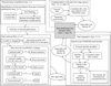 |
Fig. 2 Schematic workflow representation of the data curation process described in Sect. 2. |
| In the text | |
|
Fig. 3 Examples of SEDs from our database for different types of YSOs From top to bottom: a Class 0, a Class I, a Flat-Spectrum, a Class II. a Class III, and a Herbig AeBe star. See YSO classes discussion in Sect. 3.3. Photometric data collated by us is plotted in coloured symbols, while data points retrieved by processing data from the VizieR-SED tool are plotted contoured in black. The grey area shows the wavelength range used for deriving αIR indices in Sect. 3.3. |
| In the text | |
|
Fig. 4 Top: number of photometric data points in the SEDs collated into the NEMESIS YSO catalogue for the OSFC. Bottom: percentage of SEDs containing data points at a given wavelength range. |
| In the text | |
|
Fig. 5 Distribution IR spectral indices, αIR, estimated for sources in the NEMESIS Catalogue of YSOs in the OSFC using all photometric data available in the wavelength range 2–24 µm. Dotted lines show the limits between classes (Table 1). |
| In the text | |
|
Fig. 6 Comparison of αIR indices derived in this study (Fig. 5) with literature values from: (a) Koenig et al. (2015), (b) Großschedl et al. (2019), (c) Megeath et al. (2012), (d) Getman et al. (2017). Dashed lines reflect a 1:1 equivalence. Dotted-black lines show the limit between YSO classes adopted in this study (Table 1). |
| In the text | |
|
Fig. 7 Top: distribution of log g values collated into the NEMESIS Catalogue of YSOs in the OSFC (Sect. 3.5). Bottom: general distribution of EW values for absorption lines collected as gravity proxy. The dotted red line reflects the continuum level. Violins are shown at a fixed width for improving visualisation. Violin’s internal dotted lines reflect distributions’ first and third quartiles, and dashed lines reflect their median. |
| In the text | |
|
Fig. 8 Distribution of EWs for lines related to material inflow, out-flow and accretion in YSOs (Sect. 3.6). The dotted red line reflects the continuum level. Violins are shown at a fixed width for improving visualisation. Violin’s internal dotted lines reflect distributions’ first and third quartiles, and dashed lines reflect their median. |
| In the text | |
|
Fig. 9 Incidence of different multiplicity labels included in the NEME-SIS Catalogue of YSOs in the OSFC. Light grey bars show labels collected as part of the historical compilation (Sect. 4.1), black bars show labels collected from binary-focussed catalogues (Sect. 4.2), dark gray bars show labels attributed using Gaia DR3 data (Sect. 4.4), and red bars show labels attributed using big data approaches (Sect. 4.3). |
| In the text | |
|
Fig. 10 Distribution of the number of neighbours around sources in the NEMESIS Catalogue of YSOs in the OSFC. Results for a searching radius of 2″ are shown in red, and 5″ in black. |
| In the text | |
|
Fig. 11 RUWE as a function of variability amplitude (AGproxy) in Gaia DR3. A sample of YSOs (without known binaries and restricted to RUWE < 2.5) is divided into four magnitude bins, with different rolling quartiles shown in the left (first quartile), middle (median), and right (third quartile) panels. In all panels, the yellow dashed region and black-dashed line show the threshold for selection of unresolved pairs with RUWE adopted in this study. |
| In the text | |
|
Fig. 12 Gaia DR3 CMD for sources in the NEMESIS Catalogue of YSOs in the OSFC (shown as black dots). Blue lines show isochrones for 1 Myr (continuous line), 10 Myr (dashed line) and 1 Gyr (dotted line). The reddening direction is indicated by the black arrow, which has an AV = 1 mag length. Left: massive stars (Sect. 5.2.1) are shown as green dots. Likely MS and post-MS contaminants in our catalogue are shown as purple dots below a 20 Myr isochrone (yellow-dashed). Middle: sources are coloured by their Giant probability derived with a RF binary classifier in Appendix E. Right: sources with log ɡ collated from spectroscopic surveys (Sect. 2.3) are shown with coloured by their log ɡ measurement (Sect. 5.2.2). |
| In the text | |
|
Fig. 13 Colour-colour diagram for the yPS1 − W2cat vs. ɡPS1 − zPS1, which are two of the features used in the Extragalactic classifier discussed in Appendix E. The colour bar reflects the derived probability of a source being likely extragalactic. Black circles show extragalactic sources reported in the literature. |
| In the text | |
|
Fig. A.1 Confusion matrices for the training for the RF classifier for AllWISE’s W3 (left) and W4 (right). The top figure shows the confusion matrix for the W3 band, and the bottom figure shows the confusion matrix for the W4 band. |
| In the text | |
|
Fig. A.2 Distribution of reliability probability of AllWISE W3 and W4 magnitudes for sources in the field of the OSFC. |
| In the text | |
|
Fig. B.1 Comparison of αIR-indices estimated with (2–24 µm) and without (2–5 µm) illustrating the effect of mid-IR data availability into reported αIR-indices. Top: αIR,2–5 µm vs αIR,2–24 µm. Bottom: Fraction of under-sampled classification recovered as a function of disc class normalised by the number of sources in each class classified with the αIR,2–24 µm index. |
| In the text | |
|
Fig. E.1 Confusion matrices for the extragalactic (Left) and giant (Right) RF classifiers normalised over true labels. |
| In the text | |
|
Fig. E.2 Distribution of probabilities of sources in the field of the OSFC being extragalactic (top) and giants (bottom). The red dotted line shows the threshold for classification. |
| In the text | |
Current usage metrics show cumulative count of Article Views (full-text article views including HTML views, PDF and ePub downloads, according to the available data) and Abstracts Views on Vision4Press platform.
Data correspond to usage on the plateform after 2015. The current usage metrics is available 48-96 hours after online publication and is updated daily on week days.
Initial download of the metrics may take a while.