| Issue |
A&A
Volume 702, October 2025
|
|
|---|---|---|
| Article Number | A99 | |
| Number of page(s) | 10 | |
| Section | Stellar structure and evolution | |
| DOI | https://doi.org/10.1051/0004-6361/202554260 | |
| Published online | 10 October 2025 | |
A complex network approach to TESS light curves of δ Sct stars
1
Instituto de Astrofísica de Andalucía (CSIC), Glorieta de la Astronomía s/n, E-18008 Granada, Spain
2
Department of Physics, University of Guilan, 41335–1914 Rasht, Iran
3
Department of Physics, Faculty of Science, University of Zanjan, 45371-38791 Zanjan, Iran
⋆ Corresponding authors: This email address is being protected from spambots. You need JavaScript enabled to view it.
; This email address is being protected from spambots. You need JavaScript enabled to view it.
Received:
25
February 2025
Accepted:
8
August 2025
Abstract
Context. Complex systems are characterised by many highly interconnected dynamical units that exhibit non-linear properties. The type of pulsating stars known as δ Sct stars have intrinsic brightness variations that require non-linear models to be described comprehensively. These stars span a broad range of properties, from low to high amplitudes, as well as a broad range of complex features. We applied the complex network approach to δ Sct stars as non-linear complex systems.
Aims. Differences among the constructed networks, which might appear in the network metrics of low-amplitude and high-amplitude δ Sct stars, can indicate intrinsic asteroseismic differences that are essential for classification of pulsating stars. Additionally, the relations between the asteroseismic parameters and network metrics (such as degree or clustering distributions) can lead us to a better understanding of pulsating stars dynamics.
Methods. By using the horizontal visibility algorithm, we mapped the TESS light curves of 69 δ Sct stars to undirected horizontal visibility graphs (HVGs), where the graph nodes represent the light curve points. This allowed us to measure the morphological characteristics of HVGs, such as the distribution of links between nodes (degree distribution) and the average fraction of triangles around each node (average clustering coefficient).
Results. The average clustering coefficients for HADS and LADS display two different linear correlations with the peak-to-peak amplitude of the TESS light curves that naturally separates them into two groups. This novel approach enabled us to obtain this result without having to use an ad hoc criterion, for the first time. Exponential fits on HVG degree distributions for both HADS and LADS stars offer indices that suggest correlated stochastic generating processes for δ Sct light curves. By applying the theoretical expression for the HVGs degree distribution of random time series, we have the ability to distinguish significant pulsations from the background noise, which could become a practical tool in frequency analyses of stars going forward.
Key words: asteroseismology / methods: data analysis / stars: oscillations / stars: variables: δ Scuti
© The Authors 2025
 Open Access article, published by EDP Sciences, under the terms of the Creative Commons Attribution License (https://creativecommons.org/licenses/by/4.0), which permits unrestricted use, distribution, and reproduction in any medium, provided the original work is properly cited.
This article is published in open access under the Subscribe to Open model. This email address is being protected from spambots. You need JavaScript enabled to view it. to support open access publication.
1. Introduction
Space telescopes such as Convection, Rotation and planetary Transits (CoRoT, Baglin et al. 2009), Kepler (Gilliland et al. 2010), and Transiting Exoplanet Survey Satellite (TESS, Ricker et al. 2015) provide the most accurate light curves for seismic and exoplanets investigations. The ultra-high precision of these satellites reveals an unprecedented detail in the sinusoidal distortions of Cepheid (Christy 1964), RR Lyrae (Christy 1966), δ Sct (Stellingwerf 1980), SPB, and γ Dor stars (Kurtz et al. 2015). These are caused by non-linear mechanisms within pulsators that produce asymmetric light curves, typically with sharp ascents and slow descents of luminosity. Combination frequencies and harmonics can also appear in the frequency domain as a consequence of the non-linear response of the stellar envelope to the excited oscillations (Lares-Martiz 2022). Amplitude modulation (Bowman & Kurtz 2014), mode coupling (Barceló Forteza et al. 2015), tidally excited perturbations, binarity, and planet effects (Steindl et al. 2021), along with the non-linear driving mechanisms of modes, are complex features seen in the light curves of such stars. In the context of δ Sct stars (and particularly high-amplitude δ Sct subclass called HADS), the non-linear effects in pulsations are very significant. δ Sct stars are pulsating stars that have spectral types A0-F5 and effective temperatures between 6500 K and 9500 K. They pulsate in low-order pressure modes and they have dominant pulsation frequencies in the range of 5–80 d−1. In particular, δ Sct stars have masses in a range of 1.2 and 2.5 solar masses and they are an ideal class of pulsators for the study of different phenomena in stellar physics, since they are placed in a transition region between the fastest rotators1 among low-mass solar-like stars, with thick convective envelopes, and the slowest rotators among high-mass stars, with large convective cores and radiative envelopes (Breger 2000a; Aerts et al. 2010).
The HADS stars are classified in population I of δ Sct stars with V band amplitude ≥0.3 mag and also v sin i ≤ 30 km s−1 (Breger 2000b). In addition, Suárez et al. (2002) found a clear correlation between v sin i and oscillation amplitudes. The frequency spectrum of HADS stars mostly shows only one, two, or three independent modes, which are probably radial. This can be used to characterise these stars through period ratios versus period diagrams (Suárez et al. 2006). On the other hand, low-amplitude δ Sct stars (called LADS) pulsate in several modes with V band amplitudes of ≤0.1 mag that could be a result of their greater rotational velocities (v sin i ≃ 306 km s−1) (Breger 2007; Chang et al. 2013; Bedding et al. 2020), as detailed in Appendix A. In δ Sct stars, the well-known κ mechanism, which operates in zones of partial ionisation of hydrogen and helium, can drive low-order radial and nonradial modes of the low spherical degree to measurable amplitudes (opacity-driven unstable modes). In lower temperature δ Sct stars, near the red edge of the instability strip with substantial outer convection zones, the selection mechanism of modes with observable amplitudes could be affected by induced fluctuations of the turbulent convection. Some studies suggested the opacity-driven unstable p modes, in which non-linear processes limit their amplitudes, while intrinsically stable stochastically driven (solar-like) p modes can be excited simultaneously in the same δ Sct star (Houdek et al. 1999; Samadi et al. 2002; Antoci et al. 2011; Antoci 2014). Due to small-amplitude nonradial modes in δ Sct light curves, categorising the HADS and LADS stars is challenging.
A complex system is composed of a large number of highly interconnected individual dynamical units that exhibit emergent collective characteristics. The complex network approach could be used to classify features with the same characteristics (e.g. the degree distribution, average clustering coefficient, and shortest path length) and quantify the complexity of dynamic systems (Newman 2003, 2010; Boccaletti et al. 2006; Barabási & Pósfai 2016).
Complex network analyses have been widely applied for distinguishing individual and collective features in many different disciplines, ranging from non-linear science to biology (Barabasi & Oltvai 2004), economics (Souma et al. 2003), engineering (Ghimire et al. 2020), earthquakes (Baiesi & Paczuski 2004; Pastén et al. 2018; Vogel et al. 2020), Solar physics (Daei et al. 2017; Gheibi et al. 2017; Lotfi et al. 2020; Mohammadi et al. 2021), and stellar light curves (Muñoz & Garcés 2021). Graph theory as a powerful mathematical tool is used for creating the complex networks. In this work, we exploit the visibility graph method in order to transform light curves into complex networks (Lacasa et al. 2008). By mapping the time series into a horizontal visibility graph (Luque et al. 2009), we can capture the essential characteristics of the features into distinct individual categories.
Here, we study the characteristics of HADS and LADS stars by mapping the light curves into the graphs (or networks) using the horizontal visibility algorithm. We study the networks local and global characteristics (node degree distribution, clustering coefficients, path length, etc.) for HADS and LADS stars. Section 2 explains the sample of stars that we have used from public TESS data sets. Section 3 discusses the HVG algorithm. In Sect. 4 we show the results of the complex network analysis and discuss the insight they can provide in δ Sct stars studies. Section 5 remarks on the important findings of this study.
2. Data
TESS is the high-precision photometric instrument from NASA intended for the pursuit of Neptune- or sub-Neptune-sized planets. It scans the sky in sectors with a size of 24° ×96°, where each sector tracks two orbits of the satellite around the Earth and Moon (or about 27 days on average). TESS observes hundreds of thousands of stars at 600–1000 nm bands in a short cadence of 2 minutes and a long cadence of 30 minutes and the data are collected into Mikulski Archive for Space Telescopes (MAST)2 as both target pixels and light curve files (Ricker et al. 2015; Sullivan et al. 2015; Feinstein et al. 2019). Since a network map of a light curve requires numerous data points to obtain a picture of the fine structure details, we developed a network approach for short cadence TESS observations. Short-cadence light curves provide us with enough data points for making stable and reliable networks; in addition, they have Nyquist frequencies well above δ Sct frequencies ranges (5–80 d−1). We collected our HADS star (listed in Table B.1) from the literature and LADS stars are selected from the multimode δ Sct stars studied in (Hasanzadeh et al. 2021), listed in Table B.2. Then, we queried the pre-search data conditioning (PDC) SAP flux of light curves for 31 HADS (Table B.1) and 38 LADS (Table B.2) stars, by using the Python Lightkurve package (Lightkurve Collaboration 2018). To correct for systematic trends, the mean flux value is subtracted for each sector. Since the systematic correction tools (such as CBV-corrector) do not show significant changes in the results, we did not insist on using them.
We used the gap-filled light curves for measuring the dependence of the average shortest path length with the size of the light curves (see Sect. 4.1). Since this metric is sensitive to the size of the light curves, we filled the gaps in order to factor out their effect for different lengths of light curves. Gaps appearing in the middle of each sector, with a duration of about one day, are caused by the downlink of TESS data to Earth for processing (see TESS Instrument Handbook from Vanderspek et al. 2018 for details). To avoid the gap effects, light curves can be gap-filled by applying MIARMA (Pascual-Granado et al. 2015a, 2018), which is an open-source3 code based on interpolation using ARMA models. Then, we performed tests on three different datasets from the same light curve: original data with gaps, gap-filled data, and cut light curve (a segment corresponding to the first 6527 data points with no gap). Our tests showed that gaps can affect degree distributions, but the cut light curves behave the same as gap-filled light curves (see a comparison with Fig. C.1). Therefore, we decided to use the cut light curves for our degree distribution analyses. We also found that the average clustering shows a stable behaviour for the size of cut light curves, so we used the same-size cut light curves for the average clustering study (see Fig. 3).
3. Methods
Complex network analysis is a helpful tool for studying the characteristics of natural complex systems such as δ Sct stars, which evolve via complex dynamics. In this section, we describe how the light curves of our HADS and LADS sample stars are mapped to horizontal visibility graphs and how the graph degree distributions are characterised by different distribution functions.
3.1. Network representation of a stellar light curve
A horizontal visibility graph (HVG) focussing on the interactions of system elements is one of the visibility algorithms for building a network for a time series (Lacasa et al. 2008; Lacasa & Toral 2010; Luque et al. 2009). In mapping a time series such as a stellar light curve to a network (or a graph) via the horizontal visibility algorithm, each light curve point presents a node (vertex) in the equivalent graph. Only horizontal lines of sight between the times series points can determine the connection between the network nodes, then the nodes can be connected in pairs by lines (edges or links). Figure 1 illustrates all the connections for the first six points of the light curve (first six nodes in the equivalent graph) through undirected HVG algorithms for HD 112063 (TIC 9591460).
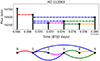 |
Fig. 1. Horizontal visibilities for the first six points of the TESS light curve of HD 112063 (TIC 9591460) δ Sct star when the points satisfy Eq. (1), shown in the upper panel. The nodes are connected in the equivalent undirected HVG based on the horizontal visibility lines, shown in the bottom panel. |
In an undirected HVG, node (ta, ya) connects to (tb, yb) if in the light curve an arbitrary point (tc, yc) such that ta < tc < tb satisfies the condition
 (1)
(1)
In the network approach, we consider networks (or graphs) instead of complex systems. A set of local and global metrics reflect particular features of these systems. Local metrics describe individual nodes or edges, along with global metrics interpret the graph as a whole. We briefly define the node degree, clustering coefficient, shortest path length, and transitivity properties of an HVG network below.
-
Degree of nodes: the node degree of a network is one of the local metrics that measures the centrality of each node. The degree of an individual node is defined as the number of edges linked to that node. Centrality displays the most influential nodes with effective connectivity through the network. In the current work, we consider the distribution of all degree of nodes for every HVG of the stellar light curve.
-
Average clustering: local and average clustering coefficients are network metrics that indicate the tendency of nodes neighbours to be clustered. The local clustering coefficient of every single node measures the fraction of complete triangles to not-completed ones including the node. It is a number between 0 and 1, such that 0 means there is no connection between the node neighbours and 1 means all neighbours are fully connected. The average clustering can be obtained by taking an average of these local values.
-
Transitivity: a global clustering coefficient that determines the density of triangles in a complex network. Transitivity is a global metric that measures the fraction of triples with their third edge serving to complete the triangle.
-
Average shortest path length: this path is another global metric for complex networks that defines the average number of links as the shortest paths for all pairs of nodes (Newman 2003, 2010; Boccaletti et al. 2006; Acosta-Tripailao et al. 2021).
3.2. Exponential distribution fits
Lacasa & Toral (2010) showed that a given time series, independent of the generating probability function, maps to an HVG with an exponential degree distribution that can be applied to explore the dynamic nature of the complex system. In this method, the exponential index (λ) can indicate the stochastic or chaotic characterisation of the generating process of the time series. We fit an exponential function (Eq. (2)) on the probability density function (PDF) of node degrees of the HVGs obtained from the light curves, expressed as
 (2)
(2)
In HVG degree distributions described by the Eq. (2), indices λ < ln(3/2) are related to more chaotic systems, while λ > ln(3/2) means that the system is governed by correlated stochastic processes that are less unpredictable. Indices equal to ln(3/2) describes an uncorrelated random process time series (Lacasa & Toral 2010; Zou et al. 2019).
We examined a hypothesis test based on Kolmogorov-Smirnov test. The null hypothesis supposes no significant difference between the degree distribution of nodes and the exponential model. However, the alternative hypothesis assumes a substantial difference between the degree distribution of nodes and the model. We calculate a p-value to decide whether or not the exponential distribution hypothesis is compatible with the distributions. A p-value lower than the threshold of 0.05 rejects the null hypothesis (H0) showing that the exponential distribution is ruled out. We cannot deny H0 for a p-value higher than the threshold of 0.05.
3.3. Lognormal distribution fits
We also applied the maximum likelihood estimation to obtain the fit parameters of a lognormal model to the HVG degree distributions due to the relation between the lognormal distributions and multiplicative mechanisms. A lognormal distribution can describe the multiplicative process with independent varying parameters (Bazarghan et al. 2008; Farhang et al. 2022), which might take place in systems having fractal features (Pietronero & Siebesma 1986), akin to what is studied for δ Sct light curves (de Franciscis et al. 2018, 2019).
The lognormal probability density function for discrete variables is introduced by
 (3)
(3)
with
 (4)
(4)
where μ and σ are the lognormal parameters. By examining a hypothesis test based on Kolmogorov–Smirnov test, we cannot reject H0 for a p-value higher than the threshold of 0.05.
4. Results and discussion
The characteristics describing the complexity of δ Sct stars can be investigated via network analysis. We applied the HVG algorithms to investigate the characteristics of 31 HADS (Table B.1) and 38 LADS (Table B.2), respectively.
4.1. δ Sct networks
Figure 2 represents the average shortest path length for the HVG of the gap-filled light curves for AD Cmi (HADS) and HD 21190 or TIC 348772511 (LADS) compared with the random network. Figure 2 shows that the average shortest path length of both stars has significantly deviated from the average shortest path length of a random network. Luque et al. (2009) proved that the HVG’s average shortest path length for any random time series is independent of the generating probability function and has a logarithmic dependence with the number of time series data points (N): 1.3log(N)−1.7. The linear dependency of the average shortest path length to the logarithm of light curve size for both cases indicated the small-world behaviour of networks (Watts & Strogatz 1998). We observed a similar behaviour for all target stars of Tables B.1 and B.2. The small-world behaviour for δ Sct stars network shows that the high peaks at the light curve are connected to several neighbouring small peaks and the other high peaks at the light curve. In the context of complex networks, small-world networks have been explored in several studies (Watts & Strogatz 1998; Mathias & Gopal 2001; Latora & Marchiori 2001).
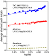 |
Fig. 2. Average shortest path length of the HVGs versus the logarithm of light curve sizes for TIC 348772511 or HD 21190 as a LADS star, AD Cmi as a HADS star, and an equivalent random network indicated by blue circles, red triangles, and olive dashed line, respectively. The fitted line for HD 21190 (blue line) and AD Cmi star (red line) deviates from the random network. |
Figure 3 depicts the average clustering coefficients of HVGs versus the light curve sizes for HADS (red lines), LADS (blue lines) stars, and also for their equivalent random networks which are so-called small worlds. The average clustering coefficient changes for small light curve sizes until a quasi-stable network is formed, and then the average clustering coefficient remains approximately constant. We cut our light curve at 6527 data points (or 9.2 days) which is shown by a black dashed line, where the average clustering property of networks seems stable and this light curve size can be used for our analysis. The size of 6527 data points (or 9.2 days) comes from the smallest segment size among our 69 light curves that does not have any gap. By considering the distribution of average clustering coefficients at the cut-line, the HVG average clustering coefficients of LADS accumulate around 0.62, which is slightly greater than 0.54 as the peak of average clustering coefficients for HADS; in addition, all stars display a considerable separation from equivalent random networks. The average clustering for equivalent small-world random networks (CR) is calculated by measuring the average node degree of each network, then divided by the number of network nodes (CR= average degree of nodes divided by number of nodes) (Watts & Strogatz 1998; Gheibi et al. 2017).
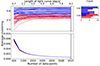 |
Fig. 3. HVG average clustering coefficients versus the graph sizes for HADS (red lines), LADS (blue lines) stars in up-left panel, and for their equivalent random networks in down-left panel. The distribution of average clustering coefficients at the size of 6527 nodes shows different maximum values for HADS (0.62) and LADS (0.54) in the up-right panel. |
Figure 4 presents the dependency of HVGs average clustering coefficients on the peak-to-peak amplitude of TESS light curves. The variety of average clustering coefficients between the same-size networks of LADS and HADS is differentiable by considering the peak-to-peak amplitudes in Fig. 4. LADS stars (blue circles) occupy higher average clustering values with a tiny range of low peak-to-peak amplitudes; however, HADS stars (red triangles) occupy lower average clustering values with higher peak-to-peak amplitudes. Average clustering is a parameter defined in the time domain which is closely related to the presence of a fine structure in the light curves (i.e. roughness). This fine structure can only be represented by a high number of frequency components (e.g. Iacobello et al. 2018). In Fig. 4, the dependence of average clustering with the peak-to-peak amplitudes shows that LADS light curves generally have a higher average clustering coefficient and it decreases for higher amplitudes. Since pulsation mode energies are also higher for higher peak-to-peak amplitude, this evidence points to a transition from high to low energies injected by the star in the oscillations favouring a few high-amplitude radial modes (low average clustering in HADS) in contrast to a high number of low-amplitude non-radial modes (high average clustering in LADS). The green circle is a LADS star (TIC 7808834) that is located nearer the transition between high clustering (LADS) and low clustering (HADS). To this end, this specific target merits an in-depth frequency analysis. Furthermore, the green triangle shows ρ Pup, which has a mono-mode HADS properties in the Fourier parameters, but its amplitude in different filters is lower than what would be expected for HADS (Nardetto et al. 2014). The current analysis with average clustering coefficient can confirm ρ Pup displays HADS properties.
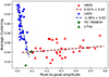 |
Fig. 4. Scatter plot of HVG average clustering versus the peak-to-peak amplitude of TESS light curves can separate the HADS (red triangles) and LADS (blue circles) in two clusters. Two linear functions (dashed lines) describe the dependency of Average clustering and peak-to-peak amplitude values as morphological parameters in network and light curve respectively. |
Figures 5 and 6 show PDFs and CDFs of degrees for HVG nodes of three HADS and three LADS stars, respectively. We fit the exponential distribution described in Sect. 3.2, to the HVG degree distributions in red lines with p-values quite higher than 0.05. Our analysis shows the robustness of exponential fits in the framework of the study Lacasa & Toral (2010), offering several hints on the physical meaning for distributions and the value of indices. Exponential indices can distinguish between the stochastic or chaotic nature of the dynamics that generate the stellar light curve as people investigate in other fields of study (Ghimire et al. 2020; Braga et al. 2016). Concerning the corresponding spatial processes of energy accumulation and discharge, exponential distributions have been found in time series for grain density of different self-organising criticality (SOC) sand-pile models (Kaki et al. 2022). By applying a robust linear regression on the logarithm of the PDF for HVG node degrees that allows two parameters to be fit as the slope and the intercept, we were able to obtain slopes higher than λ = ln(3/2). The fact that these exponential indices are higher than ln(3/2) = 0.41 might mean that the stellar brightness variations are governed by the correlated stochastic process. We calculated the exponential fits for the range of degrees k ∈ [4, +∞], with the corresponding normalisation (black dashed line PDF of node degrees in Figs. 5 and 6). We refer to Tables B.1 and B.2 for exponential indices, uncertainties, and p-values.
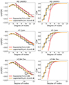 |
Fig. 5. Logarithm of PDF (first column) and CDF (second column) for the HVGs nodes degree for three HADS (HD 146953, PT Com, and V1384 Tau) stars. Exponential fits (red lines) and lognormal distributions (orange lines) are plotted on their normalised distributions in solid and dashed lines, respectively. |
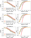 |
Fig. 6. Logarithm of PDF (first column) and CDF (second column) for the HVGs node degrees for three LADS (TIC 329153513, TIC 348772511, and TIC 459908110) stars. Exponential fits (red lines) and lognormal distributions (orange lines) are plotted on their normalised distributions in solid and dashed lines, respectively. |
In addition, we fit the PDFs and CDFs of degrees for HVG nodes of light curves with lognormal models explained in Sect. 3.3, obtaining high p-values and two distribution parameters with negligible uncertainties (Tables B.1 and B.2). In Figs. 5 and 6, the lognormal distributions are plotted in orange lines. We recall that a lognormal distribution is induced by some multiplicative stochastic process, for instance, a product of many independent stochastic variables,  . Its logarithm is a sum of many independent stochastic variables,
  , which is characterised by a Gaussian distribution. Using a heuristic argument, we observe that if node t in the HVG is linked to node t + τ, then in the corresponding time series, the height h of all nodes {t+1,…,t+τ−1} has to be lower than the height of t and t + τ. Thus, the probability P(t → t + τ) of having a link in the network between t and t + τ conditionally depends on the product
  of suitable probability functions
  of all the heights in between; in other words, it depends on the whole time story of the signal, whose values may follow distributions from independent stochastic variables. This probability P(t → t + τ) recalls a multiplicative process. Observationally, lognormal distributions have been obtained in some studies of different energetic surface phenomena in solar physics (for example Alipour et al. 2022; Farhang et al. 2022). Furthermore, we could not discard a power law behaviour for high values of degree, since (in some conditions) a lognormal distribution could switch to a power-law distribution (Mitzenmacher 2004). Following the product of probabilities argument of the former paragraph, for some specific distributions of height, PDF results in the sum of lognormal distributions, which would have essentially a lognormal body, but a power law distribution in the tail. Even in the presence of a single lognormal, if σ is an appreciable amount of the range of degree we are observing, we can confound the lognormal with power law. Finally, a small change in the constraints of multiplicative process allows for a power law distribution. As long as there is a bounded minimum that acts as a lower reflective barrier to the multiplicative model, it will yield a power law instead of a lognormal distribution. Power law distributions have been measured in models and observation of energy discharges process, such as in VG for the number of sunspots versus time Zou et al. (2014), as well as HVG for avalanche sizes in the classical SOC BTW model Adami et al. (2024).
4.2. White noise signature in the HVG networks
Luque et al. (2009) showed that the degree of nodes (k ≥ 2) for the HVG map of an uncorrelated random time series follows the theoretical exponential distribution of Eq. (5), which can be obtained from Eq. (2) when λ = ln(3/2), expressed as
 (5)
(5)
They also showed that this theoretical expression is independent of the probability distribution from which the random time series was created. Using Eq. (5), we can obtain the theoretical cumulative distribution function (CDFT) as
 (6)
(6)
The complementary cumulative distribution function (CCDF) is useful for describing the tail distributions and is related to CDF as CCDF = 1-CDF.
Figure 7 represents the PDF (top panel) and the CCDF (bottom panel) of the degrees of the HVG nodes of a Gaussian random noise with 6527 data points (the same size as our light curves) and the theoretical expression (Eqs. (5) and (6)). We expect the HVG degree distribution for any random time series with arbitrarily generated probability distribution would excellently match the theoretical expression. The Kolmogorov-Smirnov distance (KSD) is a measurement used to quantify the distance between distributions. The KSD is given by KSD = sup(|CDFdata − CDFT|), where CDFdata is the empirical cumulative distribution function (Mahmoud 2000) for the HVG degree distribution of time series. The KSD is distributed around 0.003 for various random time series with a size of 6527 data points. We suggest KSD = 0.003 as a useful criterion for distinguishing pure Gaussian white noise with a size of 6527 data points.
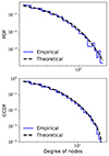 |
Fig. 7. PDF (upper panel) and CCDF (bottom panel) of the degrees of the HVG nodes of a Gaussian random time series with 6527 data points (blue line) and the theoretical functions expressed in Eqs. (5) and (6) respectively (black dashed line). |
To understand out the role played by noise on the HVG parameters of a light curve, we simulated a synthetic single-frequency time series with a size of 6527 data points in the presence of white noise with a variety of signal-to-noise ratio (S/N). The zero-S/N corresponds to a zero-amplitude signal with random Gaussian white noise (such as Fig. 2). Using the power of signal (Ps) and noise (Pn), the S/N is given by
 (7)
(7)
Figure 8 shows the KSD values for the HVG degree distributions of this synthetic noisy time series with various S/Ns. The KSD is about 0.0040 ± 0.0014 for extremely low S/Ns and it increases with increasing S/N. Increasing the S/N to slightly over than 0.1, we find the KSD becomes significantly higher than the noise network. The lower S/Ns corresponded to the lower oscillation amplitudes in the noisy background. Therefore, KSD of the HVG degree distribution of time series or light curves may be a valuable criterion for the frequency pre-whitening process. In other words, if the HVG degree distribution for a light curve residual is matched with the theoretical expression for an uncorrelated random time series, the frequency cleaning is expected to cease (see also Sect. 4.1).
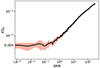 |
Fig. 8. KSD values versus the S/N for the HVG degree distributions of synthetic time series with a size of 6527 data points. The red-shaded area shows the standard deviation of KSD for several white noises. |
Figure 9 displays the CCDF of the degree nodes of the HVG networks for the same HADS star of Fig. 5 and LADS stars of Fig. 6 in the left and right columns, respectively. The Kolmogorov–Smirnov distance KSD between the HVG degree distribution of random model (black dashed line) of Eq. (6) and the HVG degree distribution of pre-whitened residuals for light curve sizes of 6527 data points were computed. The pre-whitened residuals were obtained by using SigSpec (Reegen 2012), where only the dominant frequency is removed (blue line) and all significant frequencies with S/N > 4 have been removed (red line). The green distribution corresponds to the degree distribution of the HVG of the original light curves where all frequencies are present. After removing all mode frequencies (S/N > 4), for the noisy residual of HD 146953, PT Com, and V1384 Tau, the KSD values of 0.006, 0.003, and 0.007 were obtained, respectively. Also, the KSD values for TIC 329153513, TIC 384772511, and TIC 459908110 were calculated as 0.003, 0.006, and 0.008, respectively. These results imply that the highest peak frequency is not the only mode for these HADS stars. Thus, reducing most of the oscillation modes from the δ Sct light curves gives a primarily noisy residual that approximately obeys the degree of nodes of an uncorrelated random time series.
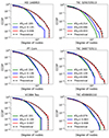 |
Fig. 9. HVG degree distributions of three HADS light curves (HD 146953, PT Com, V1384 Tau) in the left column and three LADS light curves (TIC 329153513, TIC 348772511, and TIC 459908110) in the right column. These distributions are shown in the context of all frequencies (green), in absence of the dominant frequency (blue), and in the absence of all significant frequencies (red). The black dashed line shows the theoretical expression for random series (see Eq. (6)). The KSD is presented for these three stages of pre-whitening for each star. Note: it is getting smaller and quite close to the value of 0.0040 ± 0.0014. |
The KSD about 0.004 ± 0.0014 would be a helpful criterion for verifying noisy (white) residuals by removing oscillations of a pulsating star light curve. The next steps are extending this method to other stars and applying a network approach to identify coloured noise in the residuals of the pre-whitening process.
5. Conclusions
Here, we investigate the network characteristics for δ Sct stars as non-linear complex systems. We focus on the undirected HVG’s local and global metrics to discuss the properties of HADS and LADS stars (69 sample stars listed in Tables B.1 and B.2). Our main conclusions are given below.
-
The linear dependency of the HVG average shortest path length to the logarithm of the size of δ Sct light curves (Fig. 2). This behaviour for δ Sct stars indicates the small-world complex networks with non-random properties. This small-world property implies that the peaks of the stellar flux light curves connect with some small close peaks and are then linked to other significant peaks along the light curves.
-
The average clustering coefficients of the HVGs for δ Sct stars deviate from random models and they are also different for HADS and LADS (Fig. 3). The scattering of average clustering coefficient and peak-to-peak amplitude of HADS and LADS stars can be used to separate two δ Sct subclasses in two overlapping clusters (Fig. 4) that generally follow two linear behaviours. The lower clustering coefficient for most HADS stars indicates the simpler light curve (containing one, two, or three independent modes then having a smoother light curve). In contrast, the higher clustering for LADS cases is a signature of the more complicated and rough light curve (including multiple oscillation modes and a higher chance of becoming triangles in the equivalent graph). In summary, the average clustering coefficient as a measure to the light-curve roughness in the time domain, in a similar way as connectivities were explored in (Pascual-Granado et al. 2015b), might be able to explain the higher injected energy to the HADS pulsations.
-
The nodes degree distribution of HVG networks (Figs. 5 and 6) for δ Sct stars obey the exponential distributions with indices higher than λ = ln(3/2) indicating the presence of correlated stochastic process in δ Sct light curves. The lognormal behaviour for the light curve of δ Sct stars networks also suggests a mechanism of a multiplicative generative process.
-
We find that the Kolmogorov–Smirnov distance (KSD) between the HVG nodes degree distribution of a δ Sct light curve and the analytical expression for an uncorrelated random model (with arbitrary random generation) can be an essential measure for cleaning frequencies to obtain the noisy residual of pulsating stars. The tiny KSD for a residual light curve after cleaning the frequencies may be a valuable criterion for validating the frequency analysis of pulsating stars (see Fig. 9).
In conclusion, even if in our study offers several pieces of evidence to support the exponential distribution formulation for a PDF that could be used to characterise the stochastic and chaotic behaviour of the light curves (and also study the corresponding pre-whitening cascade), our time series are short and the populations for k degree statistics have poor sampling with respect to other numerical studies (Lacasa & Toral 2010; Kaki et al. 2022; Adami et al. 2024). Further studies with longer time series are needed to either strengthen the KSD distances as a pre-whitening criterion or to verify the presence of lognormal and/or power-law distributions, as well as the underlying physical conditions where they emerge.
Noting, however, that cool stars are typically slower rotators than hot stars because their thick convective envelope undergoes angular momentum loss during their evolution (see e.g. van Saders & Pinsonneault 2013). So while rotation periods for hot stars can be less of one day, for cool stars it can become several weeks or months.
Acknowledgments
This manuscript includes data collected by the TESS mission, which are publicly available from the Mikulski Archive for Space Telescopes (MAST). Funding for the TESS mission is provided by the NASA Explorer Program. We acknowledge financial support from project PID2019-107061GB-C63 from the ‘Programas Estatales de Generación de Conocimiento y Fortalecimiento Científico y Tecnológico del Sistema de I+D+i y de I+D+i Orientada a los Retos de la Sociedad’, from project PID2023-149439NB-C42 from the ‘Proyectos de Generación de Conocimiento’ and from the Severo Ochoa grant CEX2021-001131-S funded by MICIU/AEI/10.13039/501100011033 and FEDER, EU.
References
- Acosta-Tripailao, B., Pastén, D., & Moya, P. S. 2021, Entropy, 23, 470 [NASA ADS] [CrossRef] [Google Scholar]
- Adami, V., Masoomy, H., & Nattagh-Najafi, M. 2024, ArXiv e-prints [arXiv:2412.12290] [Google Scholar]
- Aerts, C., Christensen-Dalsgaard, J., & Kurtz, D. W. 2010, Asteroseismology (Netherlands: Springer) [Google Scholar]
- Alipour, N., Safari, H., Verbeeck, C., et al. 2022, A&A, 663, A128 [NASA ADS] [CrossRef] [EDP Sciences] [Google Scholar]
- Antoci, V. 2014, in Precision Asteroseismology, eds. J. A. Guzik, W. J. Chaplin, G. Handler, & A. Pigulski, IAU Symp., 301, 333 [Google Scholar]
- Antoci, V., Handler, G., Campante, T. L., et al. 2011, Nature, 477, 570 [Google Scholar]
- Baglin, A., Auvergne, M., Barge, P., et al. 2009, in Transiting Planets, eds. F. Pont, D. Sasselov, & M. J. Holman, IAU Symp., 253, 71 [NASA ADS] [Google Scholar]
- Baiesi, M., & Paczuski, M. 2004, Phys. Rev. E, 69, 066106 [Google Scholar]
- Barabasi, A.-L., & Oltvai, Z. N. 2004, Nat. Rev. Genet., 5, 101 [Google Scholar]
- Barabási, A.-L., & Pósfai, M. 2016, Network Science (Cambridge: Cambridge University Press) [Google Scholar]
- Barceló Forteza, S., Michel, E., Roca Cortés, T., & García, R. A. 2015, A&A, 579, A133 [NASA ADS] [CrossRef] [EDP Sciences] [Google Scholar]
- Bazarghan, M., Safari, H., Innes, D. E., Karami, E., & Solanki, S. K. 2008, A&A, 492, L13 [NASA ADS] [CrossRef] [EDP Sciences] [Google Scholar]
- Bedding, T. R., Murphy, S. J., Hey, D. R., et al. 2020, Nature, 581, 147 [NASA ADS] [CrossRef] [Google Scholar]
- Boccaletti, S., Latora, V., Moreno, Y., Chavez, M., & Hwang, D.-U. 2006, Phys. Rep., 424, 175 [Google Scholar]
- Bowman, D. M., & Kurtz, D. W. 2014, MNRAS, 444, 1909 [NASA ADS] [CrossRef] [Google Scholar]
- Braga, A., Alves, L., Costa, L., et al. 2016, Phys. A: Stat. Mech. Appl., 444, 1003 [Google Scholar]
- Breger, M. 2000a, Balt. Astron., 9, 149 [Google Scholar]
- Breger, M. 2000b, ASP Conf. Ser., 210, 3 [NASA ADS] [Google Scholar]
- Breger, M. 2007, Commun. Asteroseismol., 150, 25 [NASA ADS] [CrossRef] [Google Scholar]
- Chang, S.-W., Protopapas, P., Kim, D.-W., & Byun, Y.-I. 2013, Astron. J., 145, 132 [Google Scholar]
- Christy, R. F. 1964, Rev. Mod. Phys., 36, 555 [NASA ADS] [CrossRef] [Google Scholar]
- Christy, R. F. 1966, ApJ, 144, 108 [Google Scholar]
- Daei, F., Safari, H., & Dadashi, N. 2017, ApJ, 845, 36 [Google Scholar]
- de Franciscis, S., Pascual-Granado, J., Suárez, J. C., García Hernández, A., & Garrido, R. 2018, MNRAS, 481, 4637 [Google Scholar]
- de Franciscis, S., Pascual-Granado, J., Suárez, J. C., et al. 2019, MNRAS, 487, 4457 [Google Scholar]
- Farhang, N., Shahbazi, F., & Safari, H. 2022, ApJ, 936, 87 [NASA ADS] [CrossRef] [Google Scholar]
- Feinstein, A. D., Montet, B. T., Foreman-Mackey, D., et al. 2019, PASP, 131, 094502 [Google Scholar]
- Gheibi, A., Safari, H., & Javaherian, M. 2017, ApJ, 847, 115 [NASA ADS] [CrossRef] [Google Scholar]
- Ghimire, G. R., Jadidoleslam, N., Krajewski, W. F., & Tsonis, A. A. 2020, Front. Water, 2, 17 [Google Scholar]
- Gilliland, R. L., Brown, T. M., Christensen-Dalsgaard, J., et al. 2010, PASP, 122, 131 [Google Scholar]
- Hasanzadeh, A., Safari, H., & Ghasemi, H. 2021, MNRAS, 505, 1476 [NASA ADS] [CrossRef] [Google Scholar]
- Houdek, G., Balmforth, N. J., Christensen-Dalsgaard, J., & Gough, D. O. 1999, A&A, 351, 582 [NASA ADS] [Google Scholar]
- Iacobello, G., Scarsoglio, S., & Ridolfi, L. 2018, Phys. Lett. A, 382, 1 [Google Scholar]
- Kaki, B., Farhang, N., & Safari, H. 2022, Sci. Rep., 12, 16835 [Google Scholar]
- Kurtz, D. W., Shibahashi, H., Murphy, S. J., Bedding, T. R., & Bowman, D. M. 2015, MNRAS, 450, 3015 [NASA ADS] [CrossRef] [Google Scholar]
- Lacasa, L., & Toral, R. 2010, Phys. Rev. E, 82, 036120 [Google Scholar]
- Lacasa, L., Luque, B., Ballesteros, F., Luque, J., & Nuno, J. C. 2008, PNAS, 105, 4972 [Google Scholar]
- Lares-Martiz, M. 2022, Front. Astron. Space Sci., 9, 301 [Google Scholar]
- Latora, V., & Marchiori, M. 2001, Phys. Rev. Lett., 87, 198701 [Google Scholar]
- Lightkurve Collaboration (Cardoso, J. V. d. M., et al.) 2018, Astrophysics Source Code Library [record ascl:1812.013] [Google Scholar]
- Lotfi, N., Javaherian, M., Kaki, B., Darooneh, A. H., & Safari, H. 2020, Chaos, 30, 043124 [Google Scholar]
- Luque, B., Lacasa, L., Ballesteros, F., & Luque, J. 2009, Phys. Rev. E, 80, 046103 [NASA ADS] [CrossRef] [Google Scholar]
- Mahmoud, H. 2000, Sorting: A Distribution Theory, Wiley Series in Discrete Mathematics and Optimization (Wiley) [Google Scholar]
- Mathias, N., & Gopal, V. 2001, Phys. Rev. E, 63, 021117 [Google Scholar]
- Mitzenmacher, M. 2004, Internet Math., 1, 226 [CrossRef] [Google Scholar]
- Mohammadi, Z., Alipour, N., Safari, H., & Zamani, F. 2021, J. Geophys. Res.: Space Phys., 126, e28868 [Google Scholar]
- Muñoz, V., & Garcés, N. E. 2021, Plos one, 16, e0259735 [Google Scholar]
- Nardetto, N., Poretti, E., Rainer, M., et al. 2014, A&A, 561, A151 [NASA ADS] [CrossRef] [EDP Sciences] [Google Scholar]
- Newman, M. E. 2003, SIAM Rev., 45, 167 [CrossRef] [MathSciNet] [Google Scholar]
- Newman, M. 2010, Networks: An Introduction (OUP Oxford) [Google Scholar]
- Pascual-Granado, J., Garrido, R., & Suárez, J. C. 2015a, A&A, 575, A78 [NASA ADS] [CrossRef] [EDP Sciences] [Google Scholar]
- Pascual-Granado, J., Garrido, R., & Suárez, J. C. 2015b, A&A, 581, A89 [NASA ADS] [EDP Sciences] [Google Scholar]
- Pascual-Granado, J., Suárez, J. C., Garrido, R., et al. 2018, A&A, 614, A40 [NASA ADS] [CrossRef] [EDP Sciences] [Google Scholar]
- Pastén, D., Czechowski, Z., & Toledo, B. 2018, Chaos, 28, 083128 [Google Scholar]
- Pietronero, L., & Siebesma, A. P. 1986, Phys. Rev. Lett., 57, 1098 [Google Scholar]
- Reegen, P. 2012, Commun. Asteroseismol., 163, 3 [Google Scholar]
- Ricker, G. R., Winn, J. N., Vanderspek, R., et al. 2015, J. Astron. Telesc. Instrum. Syst., 1, 014003 [Google Scholar]
- Samadi, R., Goupil, M. J., & Houdek, G. 2002, A&A, 395, 563 [NASA ADS] [CrossRef] [EDP Sciences] [Google Scholar]
- Souma, W., Fujiwara, Y., & Aoyama, H. 2003, Phys. A: Stat. Mech. Appl., 324, 396 [Google Scholar]
- Steindl, T., Zwintz, K., & Bowman, D. M. 2021, A&A, 645, A119 [NASA ADS] [CrossRef] [EDP Sciences] [Google Scholar]
- Stellingwerf, R. F. 1980, in Nonradial and Nonlinear Stellar Pulsation, eds. H. A. Hill, & W. A. Dziembowski (Germany: Springer), 125, 50 [Google Scholar]
- Suárez, J. C., Michel, E., Pérez Hernández, F., et al. 2002, A&A, 390, 523 [NASA ADS] [CrossRef] [EDP Sciences] [Google Scholar]
- Suárez, J. C., Garrido, R., & Goupil, M. J. 2006, A&A, 447, 649 [NASA ADS] [CrossRef] [EDP Sciences] [Google Scholar]
- Sullivan, P. W., Winn, J. N., Berta-Thompson, Z. K., et al. 2015, ApJ, 809, 77 [Google Scholar]
- van Saders, J. L., & Pinsonneault, M. H. 2013, ApJ, 776, 67 [Google Scholar]
- Vanderspek, R., Doty, J. P., Fausnaugh, M., et al. 2018, TESS Instrument Handbook v0.1, https://archive.stsci.edu/missions/tess/doc/TESS_Instrument_Handbook_v0.1.pdf [Google Scholar]
- Vogel, E. E., Brevis, F. G., Pastén, D., et al. 2020, Nat. Hazards Earth Syst. Sci., 20, 2943 [Google Scholar]
- Watts, D. J., & Strogatz, S. H. 1998, Nature, 393, 440 [CrossRef] [Google Scholar]
- Zou, Y., Small, M., Liu, Z., & Kurths, J. 2014, New J. Phys., 16, 013051 [Google Scholar]
- Zou, Y., Donner, R. V., Marwan, N., Donges, J. F., & Kurths, J. 2019, Phys. Rep., 787, 1 [Google Scholar]
Appendix A: HADS and LADS differences in the time domain
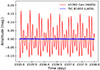 |
Fig. A.1. Three-day light curves of a HADS (V1393 Cen) and a LADS (TIC 81003) observed by TESS, respectively in red and blue. |
Appendix B: Degree distributions fitting parameters
HADS stars accompanied with the λ indices of exponential fits and their uncertainties, the p-value of exponential fits, the μ and σ of the lognormal fits, and the p-values of lognormal fits.
LADS stars accompanied with the λ indices of exponential fits and their uncertainties, the p-value of exponential fits, the μ and σ of the lognormal fits and, the p-values of lognormal fits.
Appendix C: Degree distribution differences in original, gap-filled, and cut light curves
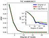 |
Fig. C.1. PDF of HVG node degrees for original light curve (solid blue), cut light curve (solid red), and gap-filled light curve (dashed green) of TIC 448892817. The distributions with logarithmic scale show the differences when the gaps exist. |
All Tables
HADS stars accompanied with the λ indices of exponential fits and their uncertainties, the p-value of exponential fits, the μ and σ of the lognormal fits, and the p-values of lognormal fits.
LADS stars accompanied with the λ indices of exponential fits and their uncertainties, the p-value of exponential fits, the μ and σ of the lognormal fits and, the p-values of lognormal fits.
All Figures
|
Fig. 1. Horizontal visibilities for the first six points of the TESS light curve of HD 112063 (TIC 9591460) δ Sct star when the points satisfy Eq. (1), shown in the upper panel. The nodes are connected in the equivalent undirected HVG based on the horizontal visibility lines, shown in the bottom panel. |
| In the text | |
|
Fig. 2. Average shortest path length of the HVGs versus the logarithm of light curve sizes for TIC 348772511 or HD 21190 as a LADS star, AD Cmi as a HADS star, and an equivalent random network indicated by blue circles, red triangles, and olive dashed line, respectively. The fitted line for HD 21190 (blue line) and AD Cmi star (red line) deviates from the random network. |
| In the text | |
|
Fig. 3. HVG average clustering coefficients versus the graph sizes for HADS (red lines), LADS (blue lines) stars in up-left panel, and for their equivalent random networks in down-left panel. The distribution of average clustering coefficients at the size of 6527 nodes shows different maximum values for HADS (0.62) and LADS (0.54) in the up-right panel. |
| In the text | |
|
Fig. 4. Scatter plot of HVG average clustering versus the peak-to-peak amplitude of TESS light curves can separate the HADS (red triangles) and LADS (blue circles) in two clusters. Two linear functions (dashed lines) describe the dependency of Average clustering and peak-to-peak amplitude values as morphological parameters in network and light curve respectively. |
| In the text | |
|
Fig. 5. Logarithm of PDF (first column) and CDF (second column) for the HVGs nodes degree for three HADS (HD 146953, PT Com, and V1384 Tau) stars. Exponential fits (red lines) and lognormal distributions (orange lines) are plotted on their normalised distributions in solid and dashed lines, respectively. |
| In the text | |
|
Fig. 6. Logarithm of PDF (first column) and CDF (second column) for the HVGs node degrees for three LADS (TIC 329153513, TIC 348772511, and TIC 459908110) stars. Exponential fits (red lines) and lognormal distributions (orange lines) are plotted on their normalised distributions in solid and dashed lines, respectively. |
| In the text | |
|
Fig. 7. PDF (upper panel) and CCDF (bottom panel) of the degrees of the HVG nodes of a Gaussian random time series with 6527 data points (blue line) and the theoretical functions expressed in Eqs. (5) and (6) respectively (black dashed line). |
| In the text | |
|
Fig. 8. KSD values versus the S/N for the HVG degree distributions of synthetic time series with a size of 6527 data points. The red-shaded area shows the standard deviation of KSD for several white noises. |
| In the text | |
|
Fig. 9. HVG degree distributions of three HADS light curves (HD 146953, PT Com, V1384 Tau) in the left column and three LADS light curves (TIC 329153513, TIC 348772511, and TIC 459908110) in the right column. These distributions are shown in the context of all frequencies (green), in absence of the dominant frequency (blue), and in the absence of all significant frequencies (red). The black dashed line shows the theoretical expression for random series (see Eq. (6)). The KSD is presented for these three stages of pre-whitening for each star. Note: it is getting smaller and quite close to the value of 0.0040 ± 0.0014. |
| In the text | |
|
Fig. A.1. Three-day light curves of a HADS (V1393 Cen) and a LADS (TIC 81003) observed by TESS, respectively in red and blue. |
| In the text | |
|
Fig. C.1. PDF of HVG node degrees for original light curve (solid blue), cut light curve (solid red), and gap-filled light curve (dashed green) of TIC 448892817. The distributions with logarithmic scale show the differences when the gaps exist. |
| In the text | |
Current usage metrics show cumulative count of Article Views (full-text article views including HTML views, PDF and ePub downloads, according to the available data) and Abstracts Views on Vision4Press platform.
Data correspond to usage on the plateform after 2015. The current usage metrics is available 48-96 hours after online publication and is updated daily on week days.
Initial download of the metrics may take a while.