| Issue |
A&A
Volume 702, October 2025
|
|
|---|---|---|
| Article Number | A178 | |
| Number of page(s) | 20 | |
| Section | Stellar structure and evolution | |
| DOI | https://doi.org/10.1051/0004-6361/202554416 | |
| Published online | 21 October 2025 | |
Investigating the metallicity dependence of the mass-loss rate relation of red supergiants
1
IAASARS, National Observatory of Athens, 15236
Penteli, Greece
2
National and Kapodistrian University of Athens, 15784
Athens, Greece
3
Institute of Astrophysics FORTH, 71110
Heraklion, Greece
4
Physics Department, University of Crete, 71003
Heraklion, Greece
5
Institute for Astronomy, University of Edinburgh, Blackford Hill, Edinburgh, EH9 3HJ
UK
6
Jet Propulsion Laboratory, California Institute of Technology, 4800 Oak Grove Drive, Pasadena, CA, 91109
USA
7
UK Astronomy Technology Centre, Royal Observatory, Blackford Hill, Edinburgh, EH9 3HJ
UK
8
IPAC, California Institute of Technology, 1200 E. California Blvd., Pasadena, CA, 91125
USA
9
Department of Physics, Maynooth University, Maynooth, Co. Kildare, Ireland
⋆ Corresponding author: This email address is being protected from spambots. You need JavaScript enabled to view it.
Received:
7
March
2025
Accepted:
1
August
2025
Abstract
Context. Red supergiants (RSGs) are cool and evolved massive stars exhibiting enhanced mass loss compared to their main sequence phase, affecting their evolution and fate. However, despite recent advances, the theory of the wind-driving mechanism is not well established and the metallicity dependence has not been determined.
Aims. We aim to uniformly measure the mass-loss rates of large samples of RSGs in different galaxies with −0.7 ≲ [Z]≲0 to investigate whether there is a potential correlation with metallicity.
Methods. We collected photometry from the ultraviolet to the mid-infrared for all our RSG candidates to construct their spectral energy distribution (SED). Our final sample includes 893 RSG candidates in the Small Magellanic Cloud (SMC), 396 in NGC 6822, 527 in the Milky Way, 1425 in M31, and 1854 in M33. Each SED was modelled using the radiative transfer code DUSTY under the same assumptions to derive the mass-loss rate.
Results. The mass-loss rates range from approximately 10−9 M⊙ yr−1 to 10−5 M⊙ yr−1, with an average value of 1.5 × 10⁻⁷ M⊙ yr−1. We provide a new mass-loss rate relation as a function of luminosity and effective temperature for both the SMC and Milky Way and compare our mass-loss rates with those derived in the Large Magellanic Cloud (LMC). The turning point in the mass-loss rate versus luminosity relation differs by around 0.2 dex between the LMC and SMC. The mass-loss rates of the Galactic RSGs at log(L/L⊙) < 4.5 are systematically lower than those determined in the other galaxies, possibly due to uncertainties in the interstellar extinction. We find 60–70% of the RSGs to be dusty, while 14% of the LMC and 2% of the SMC RSGs are significantly dusty. The results for M31 and M33 are inconclusive because of significant blending of sources at distances above 0.5 Mpc, given the resolution of Spitzer, which compromises the mid-IR photometry.
Conclusions. Overall, we find similar mass-loss rates among the galaxies, indicating no strong correlation with metallicity other than the location of the turning point. More accurate mid-IR photometry is needed to determine the metallicity dependence.
Key words: circumstellar matter / stars: evolution / stars: late-type / stars: massive / stars: mass-loss / supergiants
© The Authors 2025
 Open Access article, published by EDP Sciences, under the terms of the Creative Commons Attribution License (https://creativecommons.org/licenses/by/4.0), which permits unrestricted use, distribution, and reproduction in any medium, provided the original work is properly cited.
This article is published in open access under the Subscribe to Open model. This email address is being protected from spambots. You need JavaScript enabled to view it. to support open access publication.
1. Introduction
Red supergiants (RSGs) are cool evolved massive stars with initial masses of 8 ≲ Minit ≲ 30 M⊙ (Meynet & Maeder 2003; Heger et al. 2003). They exhibit enhanced mass loss (van Loon 2025) compared to the main sequence phase. Their winds affect the stellar evolution, their fate, the resulting type of supernovae (Eldridge et al. 2013; Yoon et al. 2017; Beasor et al. 2021; Zapartas et al. 2025), and the resulting mass of the compact object. Additionally, the winds contribute to the chemical enrichment of a galaxy, enriching it with gas and dust and contributing to star formation.
There are several hypotheses and explanations about the driving mechanism of the RSG winds, but no concrete theory yet. Radial pulsations and the highly convective envelope of RSGs are expected to contribute to this mechanism (Yoon & Cantiello 2010). However, Arroyo-Torres et al. (2015) showed that these factors alone cannot lift enough material for dust condensation. Recent studies suggest that atmospheric turbulence dominantly drives the RSG mass loss (Josselin & Plez 2007; Ohnaka et al. 2017; Kee et al. 2021). Previous empirical studies have shown that the mass-loss rates are between  for a range of luminosities (e.g. de Jager et al. 1988; van Loon et al. 2005; Goldman et al. 2017; Beasor et al. 2020; Humphreys et al. 2020; Beasor & Smith 2022; Yang et al. 2023; Antoniadis et al. 2024). These studies rely on the emission of the dust shell around the RSG in the infrared, which appears as an excess in the observed spectral energy distribution (SED). Tracing mass loss from atomic hydrogen, through the detection of the 21 cm H I line (Gérard et al. 2024), would be a more direct method. Given the weakness of the line, such a measurement has not been achieved yet.
In Antoniadis et al. (2024), we showed that the discrepancies in the mass-loss rate by two to three orders of magnitude for the same luminosity between some of these works arise from the different assumptions about the RSG mass loss mechanism and dust shell properties. We also studied one of the largest samples of RSGs to provide a more accurate mass-loss rate prescription than those that are commonly used in stellar evolution models, which are dated and based on only a few dust-enshrouded RSGs (e.g. de Jager et al. 1988; van Loon et al. 2005). Gas-dependent methods, either using CO molecular emission (Decin et al. 2024) or theoretical models (Kee et al. 2021; Fuller & Tsuna 2024), agree with our results in Antoniadis et al. (2024), providing stronger support for the assumptions we used. Zapartas et al. (2025) show that implementing prescriptions, which predict high mass-loss rates (∼10−4 M⊙ yr−1), strips off the envelope of luminous RSGs, driving them to hotter temperatures before their collapse. This can explain the low number of luminous observed RSGs but is inconsistent with the lack of luminous, yellow supernova progenitors (see Fig. 8 in Zapartas et al. 2025). Thus, quiescent steady-state RSG winds cannot strip the star of the hydrogen-rich envelope (this inability to strip was also suggested in Beasor et al. 2020). Instead, a superwind phase or outbursts occurring throughout the RSG lifetime (e.g. Decin et al. 2006; Montargès et al. 2021; Dupree et al. 2022; Munoz-Sanchez et al. 2024) or binary interaction (e.g. Ercolino et al. 2024) are necessary to strip the RSG envelope.
In contrast to the winds of hot stars that are line-driven and for which a dependence on metallicity is well established (e.g. Vink et al. 2001; Vink & de Koter 2005; Puls et al. 2008; Vink 2022), the effect of metallicity on the mass loss of RSGs is not yet clear. Previous studies found little to no effect of metallicity on the mass-loss rates, comparing results between sources from the Milky Way (MW) and the Magellanic Clouds (van Loon et al. 2005; Groenewegen et al. 2009; Mauron & Josselin 2011; Jones et al. 2012; Goldman et al. 2017). However, these studies were based on dust-enshrouded stars, including AGB stars, and either had small samples or did not analyse the different samples uniformly and comprehensively. Metallicity can affect the formation of dust around the star, and hence the radiation pressure on the dust grains, and the terminal outflow velocity (e.g. Goldman et al. 2017), but how dominant this factor is in the RSG wind is as of yet unknown. Finally, recent theoretical models of the RSG wind (Kee et al. 2021; Fuller & Tsuna 2024) did not find a strong direct dependence on metallicity. However, these studies did not investigate any indirect effects of metallicity, such as its impact on the dust shell and the RSG radius, which could contribute to the wind.
This paper aims to uniformly derive the mass-loss rates of RSGs in different metallicity environments, in the range −0.7 ≲ [Z]≲0, to determine the metallicity dependence of the RSG winds. We present an analysis of large RSG samples from the Small Magellanic Cloud (SMC), NGC 6822, the MW, M31, and M33. We then compare the results with our result for the Large Magellanic Cloud (LMC) from Antoniadis et al. (2024). In Sect. 2, we describe the sample selection for each galaxy, and in Sect. 3, we present the models and fitting methodology. We demonstrate the results in Sect. 4 and discuss and compare them in Sect. 5. Finally, we present a summary in Sect. 6.
2. Sample
To investigate the effect of metallicity on RSG mass loss, we selected Local Group galaxies with a large number of RSGs that span a range of metallicities with photometric surveys over a broad wavelength range. These include the SMC ([Z]≃ − 0.75 ± 0.3; Davies et al. 2015; Choudhury et al. 2018), NGC 6822 ([Z]= − 0.5 ± 0.2; Muschielok et al. 1999; Venn et al. 2001; Patrick et al. 2015), the MW ([Z]≃0 ± 0.2; Anders et al. 2017), M31 ([Z]≃0.13; Zurita & Bresolin 2012), and M33 ([Z]≃ − 0.18 ± 0.2; Uan et al. 2009). The results from these galaxies were then compared to the results from the LMC ([Z]= − 0.37 ± 0.14; Davies et al. 2015) from our previous study (Antoniadis et al. 2024).
2.1. SMC
We used the RSG sample from Yang et al. (2023), which is a combination of the Yang et al. (2020) and Ren et al. (2021) RSG catalogues and consists of 2121 RSG candidates, selected through photometric criteria. We additionally removed the binary RSGs from Patrick et al. (2022). Binarity could affect the assumed spherical symmetry of the dust shell, and the hot companion could destroy part of the dust, leading to an inaccurate estimation of the mass-loss rate. However, the binary candidates did not significantly affect the results in the LMC (Antoniadis et al. 2024). In this study, we removed them to have more secure mass-loss rate estimates. We used the photometry provided in the catalogue, replacing the Gaia EDR3 astrometry and photometry with Gaia DR3 (Gaia Collaboration 2016, 2023). We also excluded photometry brighter than the saturation limit of the VISTA Magellanic Cloud Survey (VMC), J ≤ 12 mag and Ks ≤ 11.5 mag. Then, we required that each source has at least one observation at a wavelength of λ > 8 μm to better constrain the infrared emission of the dust shell with our models. Furthermore, we excluded five sources with extreme values of Gaia DR3 proper motion or parallax, which are not consistent with the distribution of the sample, indicating that they are foreground stars. The final number of RSG candidates is 893. Finally, to correct for the foreground Galactic extinction, we assumed RV = 3.1 and E(B − V) = 0.04 mag (Massey et al. 2007) and the extinction law and the Aλ/AV values from Wang & Chen (2019) for each band.
2.2. Milky Way
We used the RSG catalogue from Healy et al. (2024), a compilation of literature spectroscopic RSGs and a Gaia-based method (i.e. based on the colour and magnitude of the stars in the Gaia bands). We added optical photometry from SkyMapper DR2 (Onken et al. 2019), mid-IR photometry from AllWISE (Cutri et al. 2021) with a signal-to-noise ratio of S/N > 3 in all bands, and from the Spitzer Enhanced Imaging Products (SEIP)1 with SExtractor flags ≤4 in the IRAC bands. We required there to be available photometry in at least one band in the optical, the near-IR, and the mid-IR (≥8 μm) for each source. In addition, sources that have binary flags in Healy et al. (2024) were removed. The final sample is reduced to 527 (from 651) RSGs after applying these constraints. In the case of the Galactic RSGs, we used the provided values of AV from Healy et al. (2024) to correct the foreground interstellar extinction and the values of Aλ/AV from Wang & Chen (2019) for the corresponding bands.
2.3. NGC 6822
For NGC 6822, we compiled the sample of RSG candidates from Yang et al. (2021) and Ren et al. (2021), including 234 and 465 photometric RSG candidates, respectively. We cross-matched their co-ordinates within 1″ to remove duplicates. Nally et al. (2024) identified RSG candidates using James Webb Space Telescope (JWST) photometric observations, covering the central part of the galaxy. After applying a cut at 17.4 mag on the F200W filter to exclude low-luminosity sources, we found 82 new RSG candidates that did not exist in the two previously mentioned catalogues.
We used the photometry from different surveys in Yang et al. (2021) and Ren et al. (2021), but when data were missing, we added or updated photometric data from the following surveys: Gaia DR3; Pan-STARRS1 (Chambers et al. 2016), AllWISE with ccf = 0, ex = 0 or 1 and S/N > 3 in all bands; Spitzer (Khan et al. 2015); and JWST (Nally et al. 2024). We did not use the WISEW3, W4 and Spitzer [24] bands because the angular resolution of these filters is 6.5″, 12″, and 6″, respectively, where 6″ corresponds to a radius of around 13.1 pc at the distance of NGC 6822. This led to unusually high fluxes in these bands, possibly due to blending or contamination from nearby sources. Lenkić et al. (2024) found that a large number of Spitzer-identified young stellar objects (YSOs) in this galaxy are not recovered in the JWST data due to blending, even though the case of RSGs may not be the same since they are brighter sources.
The tip of the red giant branch (TRGB) of NGC 6822 was estimated to be at 17.36 mag (Hirschauer et al. 2020) in the K band. We applied a cut at K = 16.9 mag to the sources from Ren et al. (2021), following Yang et al. (2021), to be consistent between the two samples. We additionally used the boundary at Spitzer [3.6] = 17.16 mag from Hirschauer et al. (2020), which also defines the TRGB. Only one of the sources had [3.6] mag above that limit. Then, we applied the J − K versus K cuts from Yang et al. (2021) to the photometry of all instruments available and removed the sources that did not pass the photometric constraints of at least one instrument. For the sources that did not have JWST mid-infrared photometry, we required that they at least have Spitzer [8.0]. This may not be ideal to constrain the SED during the model fitting, but as we show in the Appendix A, it can give sufficient results for the LMC (although with larger uncertainties).
We removed foreground sources using the Gaia DR3 astrometry and the method described in Maravelias et al. (2025) (similar to Maravelias et al. 2022). We additionally removed one flagged source as a quasar candidate from Gaia. Our final sample for NGC 6822 consists of 396 RSG candidates. Finally, we implemented the extinction law and values from Wang & Chen (2019) for each band with RV = 3.1 and E(B − V) = 0.22 mag (Massey et al. 2007) to correct for foreground extinction. Table 1 presents all the photometric surveys and filters used, whenever available, in each galaxy to construct the SEDs.
Photometric surveys and filters used for the SEDs in each galaxy.
2.4. M31 and M33
Wang et al. (2021) derived the mass-loss rates of more than 1000 RSG candidates near solar metallicity in M31 and M33. We used their catalogues with near-IR photometry, adding observations from Gaia DR3, AllWISE, and Spitzer (Khan et al. 2015; Khan 2017). We corrected for foreground extinction as in the other galaxies, using E(B − V) = 0.06 and 0.05 mag for M31 and M33, respectively (Massey et al. 2007). Initially, we attempted to model and recalculate the mass-loss rates with our assumptions to compare with the other galaxies. However, we found that the Spitzer and WISE photometry is not reliable at these distances (0.7 ≲ d ≲ 0.9 Mpc), providing abnormally high fluxes in the mid-IR, especially in the [24] band. We show some example SEDs in app:m31. Javadi et al. (2015) also found that the photometry of the Spitzer MIPS instrument was unreliable in M33, possibly affected by nearby sources. Javadi et al. (2013) derived mass-loss rates for RSGs in M33 using Spitzer photometry up to [8.0], which has a better resolution (∼2″) than the MIPS [24]. We tried this approach, but still found similar mass-loss rates to those we present in Appendix B. Since we are not able to evaluate the quality of the photometry, for example by comparing with data from a higher resolution instrument, and without being able to constrain the SED at longer wavelengths, we do not present these results here.
2.5. Luminosity and effective temperature
We calculated the luminosity, L, of each source by integrating its observed SED using a distance of d = 62.44 ± 1.28 kpc for the SMC (Graczyk et al. 2020), d ≃ 0.45 ± 0.01 Mpc for NGC 6822 (Górski et al. 2011; Zgirski et al. 2021), and the distances provided in Healy et al. (2024) using the estimations from Bailer-Jones et al. (2021) for the Galactic RSGs, based on the Gaia DR3 astrometry. Considering the photometric and distance errors, the log(L/L⊙) uncertainty for the RSGs in the SMC and NGC 6822 is ∼0.03 dex.
It should be mentioned that we found a luminosity of log(L/L⊙) ∼ 6 for RW Cep using a distance estimate of  kpc from Bailer-Jones et al. (2021). However, RW Cep is considered to be a member of Cep OB1 association (Melnik & Dambis 2020) at a distance of 3.4 kpc (Rate et al. 2020) or the Berkeley 94 star cluster at a distance of 3.9 kpc (Delgado et al. 2013). Thus, we adopted a distance value of 3.9 kpc for this RSG, with 3.4 and 6.7 the lower and upper limits, respectively. This demonstrates the uncertainties in the distance estimations from Bailer-Jones et al. (2021).
We used empirical relations to calculate the effective temperatures, Teff, for the SMC (Britavskiy et al. 2019):
 (1)
(1)
with an error of 140 K, and for NGC 6822 the Z-dependent relation calibrated from synthetic models from de Wit et al. (2024) (see their Table 5). In the case of Galactic RSGs, we used the Teff provided by Healy et al. (2024) which is an estimation from the spectral type, with an average error of 160 K. We present the luminosity and effective temperature distributions in a Hertzsprung–Russell (HR) diagram for all galaxies including the LMC from Antoniadis et al. (2024) along with density histograms in Fig. 1. The lines represent indicative evolutionary tracks for four different initial masses at metallicities of Z = 0.2 Z⊙ or [Z]= − 0.7 using POSYDON (Fragos et al. 2023; Andrews et al. 2024), which is a grid of MESA models (Paxton et al. 2011, 2013, 2015, 2018, 2019).
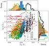 |
Fig. 1. HR diagram of the RSG samples in the LMC (blue circles), SMC (orange crosses), MW (black squares), and the NGC 6822 (green triangles). Four POSYDON evolutionary tracks for [Z]= − 0.7 and [Z] = 0 are shown in red and dotted dark red lines, respectively, and the points indicate intervals of 10 000 yr. The upper and right panels show the density histograms (areas equal to 1) of the effective temperature and luminosity, respectively. |
At lower metallicities we find higher Teff, which is expected from theory (e.g. Maeder & Meynet 2001) and has been verified from observations (e.g. Tabernero et al. 2018; González-Torà et al. 2021). However, the Teff of the Galactic RSGs can be quite uncertain since it is an estimation from the spectral type. In addition, if the spectral classifications originate from optical wavelengths, which have the TiO bands as a diagnostic, Teff could appear systematically lower (see Davies et al. 2013). The differences in luminosity between the galaxies, especially at the lower limit, originate from the different cuts and selection criteria in each galaxy. We expect most of the sources with log(L/L⊙) < 4 to be lower-mass stars; therefore, we do not consider them further.
3. Dust shell models
We used the 1D radiative transfer code DUSTY (V4)2 (Ivezić & Elitzur 1997) to model the SED of each RSG. DUSTY solves the radiative transfer equations for a central source in a spherically symmetric dust shell and we assumed that the shell extends to 104 times the inner radius, Rin. We describe the parameters and assumptions used in more detail in Antoniadis et al. (2024). We assumed a constant terminal outflow velocity, v∞, scaled with the luminosity defined in Antoniadis et al. (2024) and density distribution of the dust shell proportional to the radius as ρ ∝ r−2.
The mass-loss rate was calculated as
 (2)
(2)
where a/QV is the ratio of the dust grain radius over the extinction efficiency in the V band, ρd is the bulk density, Rin is the inner shell radius, and rgd is the gas-to-dust ratio (Beasor & Davies 2016). We assumed an average rgd for each galaxy;  (Roman-Duval et al. 2014; Clark et al. 2023) for the SMC and the typical value of
  for the MW, while in Antoniadis et al. (2024) we used rgd ≃ 300 (Clark et al. 2023). Since there is no measurement of rgd in NGC 6822 and it scales with metallicity (e.g. van Loon 2000; Li et al. 2019; Clark et al. 2023), we assumed that
  for this galaxy. We also used some nominal values for the uncertainties on rgd because they vary between studies.
We assumed a modified Mathis-Rumpl-Nordsieck (MRN) grain size distribution of n(a)∝a−q for amin ≤ a ≤ amax (Mathis et al. 1977), with amin = 0.1 μm, amax = 1 μm, and q = 3. Finally, we used the MARCS model atmospheres (Gustafsson et al. 2008) as input SEDs for the central source with typical parameters for RSGs and a metallicity of [Z]= − 0.75 for the SMC, [Z]= − 0.5 for NGC 6822, and [Z] = 0 for the MW.
We fitted the models with the observations calculating the minimum modified χ2,  (Yang et al. 2023),
![Mathematical equation: $$ \begin{aligned} \chi ^2_{\rm mod}=\frac{1}{N-p-1} \sum {\frac{[1-F(\mathrm{Model}, \lambda )/F(\mathrm{Obs}, \lambda )]^2}{F(\mathrm{Model}, \lambda )/F(\mathrm{Obs}, \lambda )}}, \end{aligned} $$](/articles/aa/full_html/2025/10/aa54416-25/aa54416-25-eq9.gif) (3)
(3)
where F(λ) is the flux at a specific wavelength, N is the number of photometric data points for each source, and p is the number of free parameters. The error models were defined as those within the minimum χmod2 + 0.002, a crude estimation of the errors from the fitting procedure, following the reasoning from Beasor et al. (2020) as we described in Antoniadis et al. (2024).
Figure 2 shows example SEDs of RSGs from each of the three galaxies of our sample. The excess at around 10 μm indicates the presence of silicate dust. The observed near-IR photometry was below the model in many model fittings of the Galactic RSGs, which we attribute to difficulties in estimating the interstellar extinction within the MW or the distance of the RSG.
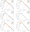 |
Fig. 2. Examples of SED fits of SMC (top row), Galactic (middle), and NGC 6822 (bottom row) RSGs. The orange diamonds show the observations and the black line is the best-fit model consisting of the attenuated flux (dashed light blue), the scattered flux (dash-dotted grey), and dust emission (dotted brown). The top left corner includes the co-ordinates of each source in degrees. Notes: All SED fit figures are available in an electronic form via https://zenodo.org/records/16736627. |
4. Results
We obtained the dust shell properties from the best-fit DUSTY models to the observed SEDs. One of the most significant properties is the optical depth, τV, which indicates how dusty a RSG is and is needed to calculate the mass-loss rate (see Eq. (2)). Figure 3 shows the histogram of the minimum χmod2 for all the galaxies of our study (and log(L/L⊙) > 4). Using the χmod2 distribution of the LMC (Antoniadis et al. 2024), which is the largest sample, we consider a good fit one with χmod2 < 1.4, the limit at roughly 3σχ2, where the standard deviation in the LMC is σχ2 = 0.41 (Antoniadis et al. 2024). We limit our results to the best-fit models with this constraint. The Galactic RSGs have a significant fraction of bad fits (39%), mainly due to uncertainties in the distance and interstellar extinction estimations. We present the dereddened photometry, the Gaia astrometry, the derived stellar and dust shell properties, and the mass-loss rates of RSGs in the SMC, MW, and NGC 6822 in the corresponding tables in Appendix C.
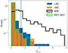 |
Fig. 3. Distribution of the minimum χmod2 for the LMC (blue bar), SMC (orange bar), MW (black line), and NGC 6822 (green line). The vertical dashed line indicates the considered limit for a good fit at χmod2 = 1.4. |
Figure 4 shows the distribution of τV for each galaxy. The LMC has more RSGs with higher values of τV than NGC 6822 and the SMC. This implies thicker dust shells and more dust production, which is expected in higher-metallicity environments. We interpret the unusually high τV values for M31 and M33 as resulting from the contamination from nearby sources due to the insufficient angular resolution of Spitzer at that distance (6″ corresponds to a radius of ∼20 pc). Thus, the derived mass-loss rates in Wang et al. (2021) were significantly affected by this factor and are not accurate. We demonstrate our results for these two galaxies in Appendix B and do not consider them further.
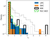 |
Fig. 4. Distribution of the minimum τV for the RSGs in the LMC (blue bar), SMC (orange bar), MW (black line), and NGC 6822 (dashed green line). The dashed and dash-dotted histograms correspond to the RSGs in M31 and M33, respectively. |
4.1. SMC
We recalculated the Ṁ of the RSGs in the SMC from Yang et al. (2023) using similar assumptions among samples to compare with the rest of the galaxies. In Fig. 5, we demonstrate the Ṁ versus L and the median absolute deviation (MAD) of W1 band from NEOWISE epoch photometry versus L for SMC. We observed a turning point or kink at around log(L/L⊙) = 4.65 and a correlation of Ṁ versus L as in Yang et al. (2023) (see their Fig. 15).
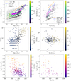 |
Fig. 5. Top: mass-loss rates vs. luminosity for SMC (left) and MW (right). The colour bar shows the Teff. The grey triangles represent the upper limits, and the open circles indicate the RSGs with spectral classifications. The magenta points correspond to the prediction of the derived Ṁ(L,Teff) relation. The dashed blue lines show the prescription from Beasor et al. (2020) for initial masses of 10 and 20 M⊙ and the dash-dotted orange line is the one from de Jager et al. (1988). Middle: MAD of W1 band vs luminosity diagram for the SMC (left) and the MW (right). The colour bar shows the mass-loss rate. Bottom: mass-loss rates vs the effective temperature for the SMC (left) and the MW (right) indicating the luminosity with colour. |
We derived a broken Ṁ relation as a function of L and Teff, similar to Antoniadis et al. (2024),
 (4)
(4)
where Ṁ is the mass-loss rate in M⊙ yr−1, L is the luminosity in L⊙, and Teff is the effective temperature in K. Table 2 includes the best-fit parameters. Figure 5 shows the prediction of the relation and the observed anti-correlation of Ṁ with Teff. We derived the relation without considering the non-dusty RSGs (upper limits with τV < 0.002, grey triangles). We also applied a cut at log(L/L⊙) = 4, approximately above the least luminous RSG with a spectroscopic classification and around the corresponding L for an 8 M⊙ star, where RSGs dominate over the lower-mass stars (see also Massey et al. 2021 and our discussion in Sect. 5.1). This limit can be slightly higher (around 4.2), but regardless, the slope does not change up to the position of the kink.
The steep dependence on the Teff is mainly because the Teff was calculated using the relation from Britavskiy et al. (2019), based on i-band measurements from Tabernero et al. (2018), which shows a steep correlation with the (J − Ks)0 colour. In addition, since the dispersion is large, the error on c2 is high. Taking into account the error on the measured Teff for each RSG, the exact value of c2 can have high uncertainties, but one can also use an average value for Teff for an L-only dependent Ṁ relation. However, our Teff dependence reproduces the results well and partly accounts for the dispersion. Mass-loss rate prescriptions are usually extrapolated to the yellow phase up to 10,000 K, but we do not suggest using our Teff dependence above around 4500 K as it would lead to negligible mass-loss rates. Using a nominal Teff to create an L-only dependent relation is more appropriate for that regime.
Furthermore, we compare our results with the prescriptions from Beasor et al. (2020) (corrected by Beasor et al. 2023) and de Jager et al. (1988). Finally, the fraction of RSGs without dust is 40% (this is an upper limit because they can reach τV > 0.002 considering the errors) and the fraction of optically thick or dusty RSGs (τV > 0.1) is 2%.
4.2. Milky Way
We show the corresponding Ṁ versus L diagram for Galactic RSGs from Healy et al. (2024) in the right panel of Fig. 5. The Ṁ is systematically lower than the other galaxies, mainly at log(L/L⊙) < 4.5. We denote with grey points those with JHKs photometry significantly lower than the best-fit model SED, as in the middle left in Fig. 2, which could result in an underestimated Ṁ, and we did not consider those in our analysis. The three outliers with high Ṁ and log(L/L⊙) < 4.5 and the three dust-free sources near log(L/L⊙) = 3 lie in ‘Region E’, denoted as less likely RSGs in Healy et al. (2024). The fraction of RSGs without dust is 32%. The middle panel of Fig. 5 also shows the MAD diagram of W1 versus L. Contrary to the LMC and SMC corresponding results, we do not observe any correlation with luminosity in this case.
Healy et al. (2024) estimated the effective temperatures from the average spectral classification. This may not be an accurate measurement, but we can still see the anti-correlation with Ṁ in the bottom part of Fig. 5. This figure also presents our derived Ṁ(L,Teff) from Eq. (4) with magenta points (using only those with a good fit of the JHKs), with best-fit parameters c1 = 1.22 ± 0.1, c2 = −24.98 ± 3.25, and c3 = −13.58 ± 0.4. The derived Ṁ relation is more uncertain than those in the LMC or SMC. The data are scarcer at high L in the MW, and the exact value of c2 can be less accurate since the Teff is estimated from the spectral type. An average value for Teff can also be used to remove its dependence.
4.3. NGC 6822
Finally, we present the Ṁ versus L of the RSG candidates in NGC 6822 in Fig. 6. We denote with orange circles the sources that have JWST Mid-Infrared Instrument (MIRI)photometry, providing more accurate results for the estimation of Ṁ. However, most sources with JWST MIRI have log(L/L⊙) < 4, and are likely lower-mass stars and not RSGs. The uncertainties are large for those without MIRI observations because their SED is constrained up to 8 μm, above which wavelength the dust emission becomes significant. The grey points indicate those without MIRI observations and log(L/L⊙) < 4, at which point the results become even more uncertain. We also show the RSGs with spectral classifications from Massey (1998), Levesque & Massey (2012), Patrick et al. (2015), and de Wit et al. (2025) and compare with the prescriptions from de Jager et al. (1988) and Beasor et al. (2020). The fraction of the RSGs without dust is 37% and the fraction of dusty RSGs is 8%.
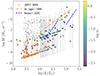 |
Fig. 6. Derived mass-loss rate as a function of the luminosity of each RSG candidate in NGC 6822. The colour bar shows the best-fit τV. RSGs with spectral classifications are outlined in black. Orange circles denote the sources that have JWST MIRI photometry. Dashed blue lines show the prescription from Beasor et al. (2020) for initial masses of 10 and 20 M⊙; the dash-dotted orange line is from de Jager et al. (1988). |
We also used a machine-learning (ML) algorithm to predict the Spitzer [24] photometry using the other Spitzer bands. In this way, we were able to constrain the model SED better. The Ṁ for luminous RSGs agrees with our result without the ML-predicted [24] band. This agreement supports our findings using observations up to [8.0]. The less luminous RSGs resulted in lower Ṁ but agreed within the uncertainties with our main result. We present the method and result in Appendix A.
We did not derive a Ṁ(L,Teff) relation for this galaxy because of the large uncertainties and there is no clear correlation with Teff. Since the metallicity is similar to the SMC, one can use our derived relation for that case. In addition, we did not find a significant correlation of the MAD of W1 with L or Ṁ because the errors of the NEOWISE W1 photometry for this galaxy are high compared to the MAD value.
5. Discussion
This work is a first step to extend the study of Yang et al. (2023) and Antoniadis et al. (2024) and uniformly study the mass-loss rates of large samples of RSGs in different metallicity environments, i.e. different galaxies. Overall, the values per luminosity bin do not vary significantly. In Antoniadis et al. (2024), we examined the effect of varying assumptions on the mass-loss mechanism and dust shell properties to resolve the large discrepancy between different studies. We chose the optimal parameters based on theory and observational constraints. However, many uncertainties can still arise, as we briefly mention in Sect. 5.3 and in more detail in Antoniadis et al. (2024).
Figure 7 compares the results from all galaxies3. The red points indicate the results from Decin et al. (2024) for five Galactic RSGs using gas diagnostics (CO rotational line emission). Their method is independent and does not rely on the properties of the dust and the SED fitting, which can lead to several uncertainties. Their results agree with ours, providing stronger support for the assumptions we used (e.g. steady-state wind, grain sizes). We found on average lower Ṁ in all galaxies than the most commonly used prescription from de Jager et al. (1988), but within the uncertainties and with a steeper slope at log(L/L⊙)≳4.5. Our results seem to agree with Beasor et al. (2023), who followed similar assumptions. Furthermore, Fuller & Tsuna (2024) developed a theoretical model for RSG mass loss, and their results agree with ours at log(L/L⊙)≳4.5. For a detailed discussion on the comparison between our results and other past works, see Antoniadis et al. (2024).
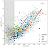 |
Fig. 7. Comparison of the mass-loss rates from all the galaxies studied: the LMC (blue circles), SMC (orange crosses), MW (black squares), and NGC 6822 (green triangles). The red points denote mass-loss rates derived from gas diagnostics. The solid lines show the prescription from Beasor et al. (2020) for initial masses of 10 and 20 M⊙, and the dash-dotted line is the relation from de Jager et al. (1988). The transparent symbols for MW and NGC 6822 indicate uncertain results. The shaded region includes stars with log(L/L⊙) < 4, which are less likely RSGs. |
We found systematically lower rates for our Galactic RSGs, mainly at log(L/L⊙)≲4.5. This may be due to uncertainties in the distances, which result in uncertain L. Furthermore, estimating the interstellar extinction within the MW is also difficult and additionally contributes to these uncertainties. In case the extinction is underestimated in the near-IR or overestimated in the optical, the models will not accurately reproduce the observed SED and result in low τV, as in the SED shown in the middle left panel of Fig. 2. To assess this issue, we obtained the extinction values using the 3D dust extinction maps from Lallement et al. (2022) and Vergely et al. (2022)4 and we found no significant differences from those presented in Healy et al. (2024).
5.1. Enhancement of mass loss: Kink
We found the position of the turning point or kink for the SMC at approximately log(L/L⊙) = 4.655 as in Yang et al. (2023), in which they used radiatively driven winds as the mass-loss mechanism assumption. This turning point is around 0.2 dex higher than the LMC. One factor that could contribute to this difference is that a lower-Z star results in a higher L for the same initial mass, as we also discussed in Antoniadis et al. (2024). Although not clear, the turning point seems to lie at the same L for NGC 6822, which is expected if it is Z-dependent. Notably, there is no clear turning point for the results in the MW, possibly due to the small number of RSGs and their higher uncertainties. There seems to be an enhancement of mass loss at roughly log(L/L⊙) = 5, as was also noticed in the Galactic sample by Humphreys et al. (2020). Furthermore, the variability of the Galactic RSGs remains roughly constant with L (see Fig. 5). This might indicate contamination of the NEOWISE photometry for several sources, making the variability not evident.
A parameter that could be responsible for the observed kink is the gas-to-dust ratio, rgd. van Loon (2025) suggests that rgd could be systematically higher for low-luminosity RSGs, meaning that the kink appears due to the assumed constant value for the whole range of L. More specifically, hotter and earlier-type RSGs could form less dust, leading to a higher rgd and vice versa. We expected this effect to also cause a noticeable shift in the Ṁ versus Teff relation, but we did not observe such a shift. In addition, according to the measurements presented in Goldman et al. (2017), rgd appears to be proportional to L, although those authors did not explicitly claim this. Other parameters could affect the rgd, so its correlation with L is not clear. The kink may also arise from a combination of different factors, such as the L/M ratio, as is suggested by Vink & Sabhahit (2023). Thus, it is difficult to determine the relevance of rgd to the kink without additional measurements of this parameter with respect to L.
We investigated whether contamination from giant stars could cause the kink, since the samples in the LMC, SMC, and NGC 6822 are photometrically classified. Asymptotic-giant-branch (AGB) stars have high mass-loss rates and could appear at the higher end of Ṁ versus L at log(L/L⊙)≲4.5, creating an artificial turning point or kink (although AGB stars also span a wide range of Ṁ similar to RSGs). We assessed this in two ways. First, we examined the mass-loss rate relation of confirmed RSGs (i.e. with spectral classifications) in the SMC and LMC to verify the turning point. In the LMC, there are not many spectroscopic observations at log(L/L⊙)≲4.4, so, in this case, we cannot distinguish a kink. In the SMC, there are more observations at log(L/L⊙)≲4.6 to confirm the presence of a kink. We show Ṁ versus L and the MAD diagram for the SMC in Figs. 8 and 9. In both figures, especially in the MAD diagram of W1, we observe a turning point at log(L/L⊙)≃4.65, although in the Ṁ(L) relation the uncertainties of the Ṁ are significant. The presence of the kink for the spectrally classified RSGs implies that AGB contamination is not causing it. We demonstrate the fitted relation on the spectroscopic data assuming a broken law or a linear relation for the SMC in Appendix D.
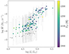 |
Fig. 8. Mass-loss rates of RSGs in the SMC with spectroscopic classifications from the literature. Triangles indicate upper limits and the colour indicates the effective temperature using Eq. (1). |
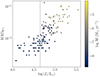 |
Fig. 9. Median-absolute-deviation (MAD) diagram of W1 band of RSGs in the SMC with spectroscopic classifications from the literature. The colour indicates the corresponding mass-loss rates. The vertical dashed line shows the position of the kink from Fig. 5 at log(L/L⊙) = 4.65. |
Second, we quantified the contamination from giant stars with the same colours as RSGs in the MW to use it as a probe for the other galaxies. Healy et al. (2024) compiled both a catalogue of all spectrally classified K and M-type stars in the MW and a final catalogue consisting of only RSGs. This means that the initial sample included AGB stars with similar Teff (and colour) as RSGs. Since our RSG samples in the LMC and SMC are defined from colour-magnitude diagrams (CMDs), i.e. the colour of the sources, we used their full (“all late-type bright stars”) catalogue to calculate the fraction of RSGs over the total number of all K or M-type stars in the MW in the range 3.6 ≤ log(L/L⊙) < 4.5. Figure 10 presents this fraction as a function of L. We found that RSGs consist of around 70% of the total sample at log(L/L⊙) = 4 and this fraction increases with increasing L. At 3.8 ≤ log(L/L⊙) < 4, the fraction drops to around 20–40%. We should note that the same initial mass corresponds to a higher L at lower metallicity. This means that the corresponding fraction of 70% RSGs at log(L/L⊙) ∼ 4 in the MW could be around log(L/L⊙) ∼ 4.3 for the LMC or 4.4 for the SMC.
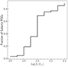 |
Fig. 10. Fraction of the Galactic RSGs from Healy et al. (2024) over the total number of K or M-type bright stars from their initial sample. |
According to Healy et al. (2024), their sources at 3.36 < log(L/L⊙) < 3.92 at what they defined as ‘Region C’ in the HR diagram (see their Figs. 4 and 5) consist of intermediate-mass AGB stars, which are 4.9% of the total AGB sample, and lower-mass (∼9 M⊙) RSGs, which consist of almost 0% of the total RSG sample6. However, they mention that this region is biased against observations of RSGs. Hence, it is difficult to robustly quantify the AGB contamination in this range of L and probe it to the corresponding region in the LMC and SMC. Furthermore, we estimated the mass-loss rates for the whole catalogue of all bright late-type stars from Healy et al. (2024) to examine if an artificial turning point is created from AGB stars and we found no such indication. Similarly, Goldman et al. (2017) included lower-L Galactic AGB stars and higher-L LMC RSGs in their study but did not observe a turning point to justify such an argument (see their Fig. 20).
Finally, Neugent et al. (2020) mention that the strong AGB contamination is up to log(L/L⊙) = 4 in M31, above which point there is a distinct stellar population in the J − Ks CMD (see their Fig. 8). This limit could be around 4.2–4.3 if we want to be more conservative. Our analysis shows that the AGB contamination cannot be that significant to create an artificial kink. Further spectroscopic observations at 4 < log(L/L⊙) < 4.5 of our studied LMC and SMC photometric RSG samples would resolve this issue.
5.2. The metallicity dependence
Overall, we found no strong correlation between the mass-loss rate and metallicity. Considering the uncertainties of the results from the MW, it is difficult to determine the metallicity dependence of RSG mass loss accurately. The shift of the kink by around 0.2 dex in luminosity between the LMC and SMC might be due to metallicity, as is also mentioned by Wen et al. (2024). However, we could attribute part of it to the different resulting luminosity for the same initial mass at a different metallicity. We compare the distribution of Ṁ for each galaxy for log(L/L⊙) > 4.5, so that we remove all the uncertainties or biases regarding the kink, in Fig. 11. The distributions seem to agree without clear differences. However, the LMC has several sources with higher Ṁ. Table 3 presents the median and mean values of the Ṁ and other parameters for each galaxy. Correspondingly, Fig. 12 shows the median, Ṁ, as a function of Z for all RSGs (log(L/L⊙) > 4) and for high L RSGs (log(L/L⊙) > 4.5). The error bars on the y axis correspond to the deviation on the median. The median, Ṁ, of the LMC appears to be slightly higher than the SMC, likely due to the position of the turning point at lower L creating a steeper slope after that point. However, everything lies within the uncertainties of the gas-to-dust ratio, which is significant for the SMC, and the dispersion of the Ṁ.
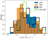 |
Fig. 11. Distribution of the mass-loss rate of RSGs with log(L/L⊙) > 4.5 for the LMC (blue bar), SMC (orange bar), MW (black line), and NGC 6822 (dashed green line). |
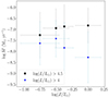 |
Fig. 12. Median mass-loss rate vs. metallicity for each galaxy of our study and two luminosity ranges. |
Finally, we performed a Kolmogorov–Smirnov (KS) test on the Ṁ distributions with log(L/L⊙) > 4.5 to assess if two samples originate from the same distribution. We found a p value of 5 × 10⁻⁵ for the LMC and SMC, indicating a significant difference, implying a Z-dependence. However, this may not be completely valid for two reasons. First, the KS test is more sensitive close to the centres of the distributions, rather than the whole shapes. Second, the different positions of the kink and the assumption of an average gas-to-dust ratio could contribute to that difference. The combinations of the other galaxies result in p > 0.1, so we cannot reject the null hypothesis.
Previous studies (van Loon et al. 2005; Groenewegen et al. 2009; Goldman et al. 2017) concluded that metallicity had little to no effect on the Ṁ studying samples consisting of both RSGs and AGB stars. However, these studies had significantly smaller samples than ours. In addition, Mauron & Josselin (2011) suggested a scaling of  to the de Jager et al. (1988) relation derived from Galactic RSGs. However, they considered small samples of RSGs in the SMC and LMC from Bonanos et al. (2010), who estimated the mass-loss rates using a different method from de Jager et al. (1988).
Metallicity could affect the dust-driven wind. Kee et al. (2021) developed a theoretical model for the RSG mass loss assuming turbulent pressure as the dominant mechanism behind it, which is not strongly dependent on metallicity. However, metallicity affects dust production and if radiation pressure on the dust grains becomes important, metallicity could play a role. Similarly, the theoretical model of Fuller & Tsuna (2024) does not directly depend on metallicity, but they did not investigate its role on the dust shell. Finally, Goldman et al. (2017) found a metallicity correlation with the outflow velocity but the effect was mostly cancelled out with the anti-correlation of the gas-to-dust ratio.
More dust is expected to form in higher-metallicity environments. In Fig. 4, we observe that τV increases with increasing Z, which is also depicted in the mean τV in Table 3. Figure 13 demonstrates the distribution of the dust-production rate, Ṁd, for RSGs with log(L/L⊙) > 4, which we calculated from Eq. (2), removing the factor of rgd. As in the distribution of τV, the dust-production rate is higher with increasing Z. However, this is not clear for the Galactic RSGs, which have a wide range of Ṁd, and it is quite low, especially at log(L/L⊙) < 4.5 compared to the other galaxies. This could arise from the uncertainties of the Galactic RSG results we mentioned and the reason that the data are scarcer at high L compared to the SMC and LMC. The trend of Ṁd with Z becomes clearer at log(L/L⊙) > 4.5, as we examined. Furthermore, considering dusty RSGs to be those with τV > 0.1, we found 14% of the RSGs in the LMC and 2% of the RSGs in the SMC to be dusty. This agrees with the value of 12% reported by de Wit et al. (2024) for RSGs at subsolar metallicity (defining the dusty ones as [3.6]−[4.5]> 0.1 mag). Finally, we show mid-IR colour (related to dust emission) diagrams with respect to the Ṁ in app:colour.
Properties of RSGs with log(L/L⊙) > 4 in each galaxy
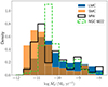 |
Fig. 13. Distribution of the dust-production rate of RSGs with log(L/L⊙) > 4 for the LMC (blue bar), SMC (orange bar), MW (black line), and NGC 6822 (dashed green line). |
5.3. Caveats
The caveats regarding the estimation of mass-loss rates from the properties of the dust shell, the SED fitting, and the different assumptions (grain size, gas-to-dust ratio, wind mechanism) have been described in Antoniadis et al. (2024). We assumed a uniform average value of rgd, which can vary within a galaxy and for RSGs with different L, especially in the SMC where it can reach values of up to around 10 000 (Clark et al. 2023). We also assumed an average Z, which can vary between RSGs in the same host galaxy (e.g. Davies et al. 2015). Nevertheless, we could distinguish the overall trend by studying large populations of RSGs. There seems to be a negligible upward trend in Fig. 12. However, if the Z dependence is minor compared to the mentioned uncertainties in Ṁ, it becomes more difficult to accurately compare RSGs from different galaxies and draw a concrete conclusion.
6. Summary
We compared the mass-loss rates of the largest sample of RSGs in four galaxies with different metallicity environments: the SMC, MW, NGC 6822, and the LMC; the results of the LMC were from Antoniadis et al. (2024). We measured the dust shell properties and mass-loss rates by fitting the observed SEDs with models from the radiative transfer code DUSTY. The mass-loss rates range from approximately 10−9 M⊙ yr−1 to 10−5 M⊙ yr−1, with an average value of around 1.5 × 10⁻⁷ M⊙ yr−1. There is no evidence of a significant correlation with metallicity, apart from the shift of the kink by 0.2 dex in the Ṁ(L) relation between the LMC and SMC. Concerning the sample of Galactic RSGs, there is no clear indication of a kink. However, the results from the Galactic RSGs are inconclusive due to uncertainties in the distance and interstellar extinction estimations, while the results of NGC 6822 have uncertainties due to worse mid-IR photometric quality from Spitzer at that distance.
We derived Ṁ relations as a function of L and Teff for the SMC and MW, and relations using only the spectroscopic RSGs in the LMC and SMC. We excluded the upper limits in the derivation of these relations; thus, they are valid for RSGs with dust (τV ≥ 0.002). The Ṁ(L) relation of the spectroscopic RSGs in the SMC indicates the presence of a kink, but more observations are needed to confirm it. Using the sample from Healy et al. (2024), we showed that RSGs dominate the stellar population at log(L/L⊙) > 4 in the MW, implying that the kink does not arise from AGB contamination. However, this limit may be at a higher L for lower metallicities. Moreover, we confirmed that metallicity affects the formation of dust by showing that the optical depth of the dust shell of RSGs in higher-Z galaxies is larger on average. This could mean that radiation pressure on the dust shell becomes more significant at higher Z and would result in higher mass-loss rates if this force were dominant in the driving of the wind.
Considering the dust properties of the RSG sample, we found that 30–40% of the RSGs in all the galaxies do not have any dust, most of which have log(L/L⊙)≲4.7. Also, 14% of the RSGs in the LMC and 2% of the RSGs in the SMC were found to be significantly dusty (τV > 0.1). Finally, we studied RSG samples in M31 and M33, but the Spitzer photometry, especially at [24], becomes unreliable at these distances (d > 0.5 Mpc). JWST data will enable RSGs in galaxies of different metallicities to be investigated with higher-quality mid-IR photometry and resolve the metallicity dependence of the RSG mass-loss rates.
Data availability
All SED fit figures are available in an electronic form via https://zenodo.org/records/16736627. Tables C.1, C.2, and C.3 are available at the CDS via https://cdsarc.cds.unistra.fr/viz-bin/cat/J/A+A/702/A178
The foreground extinction correction for AKARI S11 in Antoniadis et al. (2024) was incorrect, leading to a slight overestimation of the Ṁ for the sources that had this photometric data point. Those sources were around 30% of the total catalogue of the LMC, and we found that it did not affect the overall trend of the Ṁ(L) relation. Figure 7 shows the results for the corrected value.
Available through the G-Tomo tool https://explore-platform.eu/sda/g-tomo
We refer to the position of the kink as the point where the higher end of Ṁ creates a “turn” as a function of L. Due to the dispersion of Ṁ at a specific L, this point occupies the region around 4.6 < log(L/L⊙) < 5.
Healy et al. (2024) reports these values but in their Fig. 4 there are 5 out of 156 RSGs, which would correspond to around 3%. This applies similarly to the AGB stars and their fractions, which are probably typos. In any case, for our discussion, these regions consist of small fractions of RSGs and intermediate-mass AGB stars.
These values correspond to the mean values from all available resources as found in the NED - NASA/IPAC Extragalactic Database (accessed, July 24, 2024), for each galaxy. They might slightly differ from the distances used in the main part of the paper, but do not affect the result.
The mean values for the SMC and NGC 6822 are 9.60 mag and 10.19 mag for IRAC1, 9.59 mag and 10.03 mag for IRAC2, 9.45 mag and 9.90 mag for IRAC3, 9.34 mag and 9.86 mag for IRAC4, 9.02 mag and 7.36 mag for MIPS [24] band, for each galaxy, respectively. The mean values of the JWST [21] band (yellow) and our predictions for [24] (red) are found at 10.29 mag and 9.58 mag, respectively.
Acknowledgments
KA, AZB, GMS, and GM acknowledge funding support from the European Research Council (ERC) under the European Union’s Horizon 2020 research and innovation program (“ASSESS”, Grant agreement No. 772086). EZ acknowledges support from the Hellenic Foundation for Research and Innovation (H.F.R.I.) under the “3rd Call for H.F.R.I. Research Projects to Support Post-Doctoral Researchers” (Project No: 7933). This work is based in part on observations made with the NASA/ESA/CSA James Webb Space Telescope. The data were obtained from the Mikulski Archive for Space Telescopes at the Space Telescope Science Institute, which is operated by the Association of Universities for Research in Astronomy, Inc., under NASA contract NAS 5-03127 for JWST. These observations are associated with program #1234. We thank Stephan de Wit for his presence and feedback throughout a significant part of this work, Emma Beasor and Nathan Smith for valuable discussions regarding the analysis of the results, Sarah Healy for answering questions about their Galactic RSG catalogue, and Despina Hatzidimitriou for discussions on the results. Finally, we thank the referee, Dr. Jacco van Loon, for his valuable comments and suggestions.
References
- Anders, F., Chiappini, C., Minchev, I., et al. 2017, A&A, 600, A70 [NASA ADS] [CrossRef] [EDP Sciences] [Google Scholar]
- Andrews, J. J., Bavera, S. S., Briel, M., et al. 2024, ArXiv e-prints [arXiv:2411.02376] [Google Scholar]
- Antoniadis, K., Bonanos, A. Z., de Wit, S., et al. 2024, A&A, 686, A88 [NASA ADS] [CrossRef] [EDP Sciences] [Google Scholar]
- Arroyo-Torres, B., Wittkowski, M., Chiavassa, A., et al. 2015, A&A, 575, A50 [NASA ADS] [CrossRef] [EDP Sciences] [Google Scholar]
- Bailer-Jones, C. A. L., Rybizki, J., Fouesneau, M., Demleitner, M., & Andrae, R. 2021, AJ, 161, 147 [Google Scholar]
- Beasor, E. R., & Davies, B. 2016, MNRAS, 463, 1269 [NASA ADS] [CrossRef] [Google Scholar]
- Beasor, E. R., & Smith, N. 2022, ApJ, 933, 41 [NASA ADS] [CrossRef] [Google Scholar]
- Beasor, E. R., Davies, B., Smith, N., et al. 2020, MNRAS, 492, 5994 [Google Scholar]
- Beasor, E. R., Davies, B., & Smith, N. 2021, ApJ, 922, 55 [NASA ADS] [CrossRef] [Google Scholar]
- Beasor, E. R., Davies, B., Smith, N., et al. 2023, MNRAS, 524, 2460 [Google Scholar]
- Bonanos, A. Z., Lennon, D. J., Köhlinger, F., et al. 2010, AJ, 140, 416 [NASA ADS] [CrossRef] [Google Scholar]
- Britavskiy, N., Lennon, D. J., Patrick, L. R., et al. 2019, A&A, 624, A128 [NASA ADS] [CrossRef] [EDP Sciences] [Google Scholar]
- Chambers, K. C., Magnier, E. A., Metcalfe, N., et al. 2016, ArXiv e-prints [arXiv:1612.05560] [Google Scholar]
- Choudhury, S., Subramaniam, A., Cole, A. A., & Sohn, Y. J. 2018, MNRAS, 475, 4279 [NASA ADS] [CrossRef] [Google Scholar]
- Clark, C. J. R., Roman-Duval, J. C., Gordon, K. D., et al. 2023, ApJ, 946, 42 [NASA ADS] [CrossRef] [Google Scholar]
- Cutri, R. M., Wright, E. L., Conrow, T., et al. 2021, VizieR Online Data Catalog: II/328 [Google Scholar]
- Davies, B., Kudritzki, R.-P., Plez, B., et al. 2013, ApJ, 767, 3 [Google Scholar]
- Davies, B., Kudritzki, R.-P., Gazak, Z., et al. 2015, ApJ, 806, 21 [NASA ADS] [CrossRef] [Google Scholar]
- de Jager, C., Nieuwenhuijzen, H., & van der Hucht, K. A. 1988, A&AS, 72, 259 [NASA ADS] [Google Scholar]
- de Wit, S., Bonanos, A. Z., Antoniadis, K., et al. 2024, A&A, 689, A46 [NASA ADS] [CrossRef] [EDP Sciences] [Google Scholar]
- de Wit, S., Muñoz-Sanchez, G., Maravelias, G., et al. 2025, A&A, 698, A279 [NASA ADS] [CrossRef] [EDP Sciences] [Google Scholar]
- Decin, L., Hony, S., de Koter, A., et al. 2006, A&A, 456, 549 [NASA ADS] [CrossRef] [EDP Sciences] [Google Scholar]
- Decin, L., Richards, A. M. S., Marchant, P., & Sana, H. 2024, A&A, 681, A17 [NASA ADS] [CrossRef] [EDP Sciences] [Google Scholar]
- Delgado, A. J., Djupvik, A. A., Costado, M. T., & Alfaro, E. J. 2013, MNRAS, 435, 429 [Google Scholar]
- Dupree, A. K., Strassmeier, K. G., Calderwood, T., et al. 2022, ApJ, 936, 18 [NASA ADS] [CrossRef] [Google Scholar]
- Eldridge, J. J., Fraser, M., Smartt, S. J., et al. 2013, MNRAS, 436, 774 [NASA ADS] [CrossRef] [Google Scholar]
- Ercolino, A., Jin, H., Langer, N., & Dessart, L. 2024, A&A, 685, A58 [NASA ADS] [CrossRef] [EDP Sciences] [Google Scholar]
- Fragos, T., Andrews, J. J., Bavera, S. S., et al. 2023, ApJS, 264, 45 [NASA ADS] [CrossRef] [Google Scholar]
- Fuller, J., & Tsuna, D. 2024, Open J. Astrophys., 7, 47 [CrossRef] [Google Scholar]
- Gaia Collaboration (Prusti, T., et al.) 2016, A&A, 595, A1 [NASA ADS] [CrossRef] [EDP Sciences] [Google Scholar]
- Gaia Collaboration (Vallenari, A., et al.) 2023, A&A, 674, A1 [NASA ADS] [CrossRef] [EDP Sciences] [Google Scholar]
- Gérard, E., van Driel, W., Matthews, L. D., et al. 2024, A&A, 692, A54 [NASA ADS] [CrossRef] [EDP Sciences] [Google Scholar]
- Goldman, S. R., van Loon, J. T., Zijlstra, A. A., et al. 2017, MNRAS, 465, 403 [Google Scholar]
- González-Torà, G., Davies, B., Kudritzki, R.-P., & Plez, B. 2021, MNRAS, 505, 4422 [CrossRef] [Google Scholar]
- Górski, M., Pietrzyński, G., & Gieren, W. 2011, AJ, 141, 194 [Google Scholar]
- Graczyk, D., Pietrzyński, G., Thompson, I. B., et al. 2020, ApJ, 904, 13 [Google Scholar]
- Groenewegen, M. A. T., Sloan, G. C., Soszyński, I., & Petersen, E. A. 2009, A&A, 506, 1277 [NASA ADS] [CrossRef] [EDP Sciences] [Google Scholar]
- Gustafsson, B., Edvardsson, B., Eriksson, K., et al. 2008, A&A, 486, 951 [NASA ADS] [CrossRef] [EDP Sciences] [Google Scholar]
- Healy, S., Horiuchi, S., Colomer Molla, M., et al. 2024, MNRAS, 529, 3630 [NASA ADS] [CrossRef] [Google Scholar]
- Heger, A., Fryer, C. L., Woosley, S. E., Langer, N., & Hartmann, D. H. 2003, ApJ, 591, 288 [CrossRef] [Google Scholar]
- Hirschauer, A. S., Gray, L., Meixner, M., et al. 2020, ApJ, 892, 91 [Google Scholar]
- Humphreys, R. M., Helmel, G., Jones, T. J., & Gordon, M. S. 2020, AJ, 160, 145 [NASA ADS] [CrossRef] [Google Scholar]
- Ivezić, Z., & Elitzur, M. 1997, MNRAS, 287, 799 [CrossRef] [Google Scholar]
- Javadi, A., van Loon, J. T., Khosroshahi, H., & Mirtorabi, M. T. 2013, MNRAS, 432, 2824 [NASA ADS] [CrossRef] [Google Scholar]
- Javadi, A., Saberi, M., van Loon, J. T., et al. 2015, MNRAS, 447, 3973 [Google Scholar]
- Jones, O. C., Kemper, F., Sargent, B. A., et al. 2012, MNRAS, 427, 3209 [Google Scholar]
- Josselin, E., & Plez, B. 2007, A&A, 469, 671 [NASA ADS] [CrossRef] [EDP Sciences] [Google Scholar]
- Kee, N. D., Sundqvist, J. O., Decin, L., de Koter, A., & Sana, H. 2021, A&A, 646, A180 [NASA ADS] [CrossRef] [EDP Sciences] [Google Scholar]
- Khan, R. 2017, ApJS, 228, 5 [NASA ADS] [CrossRef] [Google Scholar]
- Khan, R., Stanek, K. Z., Kochanek, C. S., & Sonneborn, G. 2015, ApJS, 219, 42 [NASA ADS] [CrossRef] [Google Scholar]
- Lallement, R., Vergely, J. L., Babusiaux, C., & Cox, N. L. J. 2022, A&A, 661, A147 [NASA ADS] [CrossRef] [EDP Sciences] [Google Scholar]
- Lenkić, L., Nally, C., Jones, O. C., et al. 2024, ApJ, 967, 110 [CrossRef] [Google Scholar]
- Levesque, E. M., & Massey, P. 2012, AJ, 144, 2 [CrossRef] [Google Scholar]
- Li, Q., Narayanan, D., & Davé, R. 2019, MNRAS, 490, 1425 [CrossRef] [Google Scholar]
- Li, Z.-W., Yang, M., Jiang, B., & Ren, Y. 2025, ApJ, 979, 208 [Google Scholar]
- Maeder, A., & Meynet, G. 2001, A&A, 373, 555 [NASA ADS] [CrossRef] [EDP Sciences] [Google Scholar]
- Maravelias, G., Bonanos, A. Z., Antoniadis, K., et al. 2025, A&A, submitted [arXiv:2504.01232] [Google Scholar]
- Maravelias, G., Bonanos, A. Z., Tramper, F., et al. 2022, A&A, 666, A122 [NASA ADS] [CrossRef] [EDP Sciences] [Google Scholar]
- Massey, P. 1998, ApJ, 501, 153 [Google Scholar]
- Massey, P. 2002, ApJS, 141, 81 [NASA ADS] [CrossRef] [Google Scholar]
- Massey, P., Neugent, K. F., Levesque, E. M., Drout, M. R., & Courteau, S. 2021, AJ, 161, 79 [NASA ADS] [CrossRef] [Google Scholar]
- Massey, P., Olsen, K. A. G., Hodge, P. W., et al. 2007, AJ, 133, 2393 [Google Scholar]
- Mathis, J. S., Rumpl, W., & Nordsieck, K. H. 1977, ApJ, 217, 425 [Google Scholar]
- Mauron, N., & Josselin, E. 2011, A&A, 526, A156 [CrossRef] [EDP Sciences] [Google Scholar]
- Melnik, A. M., & Dambis, A. K. 2020, MNRAS, 493, 2339 [NASA ADS] [CrossRef] [Google Scholar]
- Meynet, G., & Maeder, A. 2003, A&A, 404, 975 [NASA ADS] [CrossRef] [EDP Sciences] [Google Scholar]
- Montargès, M., Cannon, E., Lagadec, E., et al. 2021, Nature, 594, 365 [Google Scholar]
- Munoz-Sanchez, G., de Wit, S., Bonanos, A. Z., et al. 2024, A&A, 690, A99 [NASA ADS] [CrossRef] [EDP Sciences] [Google Scholar]
- Muschielok, B., Kudritzki, R. P., Appenzeller, I., et al. 1999, A&A, 352, L40 [NASA ADS] [Google Scholar]
- Nally, C., Jones, O. C., Lenkić, L., et al. 2024, MNRAS, 531, 183 [NASA ADS] [CrossRef] [Google Scholar]
- Neugent, K. F., Levesque, E. M., Massey, P., Morrell, N. I., & Drout, M. R. 2020, ApJ, 900, 118 [CrossRef] [Google Scholar]
- Ohnaka, K., Weigelt, G., & Hofmann, K. H. 2017, Nature, 548, 310 [Google Scholar]
- Onken, C. A., Wolf, C., Bessell, M. S., et al. 2019, PASA, 36, e033 [Google Scholar]
- Patrick, L. R., Evans, C. J., Davies, B., et al. 2015, ApJ, 803, 14 [Google Scholar]
- Patrick, L. R., Thilker, D., Lennon, D. J., et al. 2022, MNRAS, 513, 5847 [Google Scholar]
- Paxton, B., Bildsten, L., Dotter, A., et al. 2011, ApJS, 192, 3 [Google Scholar]
- Paxton, B., Cantiello, M., Arras, P., et al. 2013, ApJS, 208, 4 [Google Scholar]
- Paxton, B., Marchant, P., Schwab, J., et al. 2015, ApJS, 220, 15 [Google Scholar]
- Paxton, B., Schwab, J., Bauer, E. B., et al. 2018, ApJS, 234, 34 [NASA ADS] [CrossRef] [Google Scholar]
- Paxton, B., Smolec, R., Schwab, J., et al. 2019, ApJS, 243, 10 [Google Scholar]
- Puls, J., Vink, J. S., & Najarro, F. 2008, A&ARv, 16, 209 [NASA ADS] [CrossRef] [Google Scholar]
- Rate, G., Crowther, P. A., & Parker, R. J. 2020, MNRAS, 495, 1209 [NASA ADS] [CrossRef] [Google Scholar]
- Ren, Y., Jiang, B., Yang, M., Wang, T., & Ren, T. 2021, ApJ, 923, 232 [NASA ADS] [CrossRef] [Google Scholar]
- Roman-Duval, J., Gordon, K. D., Meixner, M., et al. 2014, ApJ, 797, 86 [NASA ADS] [CrossRef] [Google Scholar]
- Tabernero, H. M., Dorda, R., Negueruela, I., & González-Fernández, C. 2018, MNRAS, 476, 3106 [NASA ADS] [CrossRef] [Google Scholar]
- Uan, V., Urbaneja, M. A., Kudritzki, R.-P., et al. 2009, ApJ, 704, 1120 [CrossRef] [Google Scholar]
- van Loon, J. T. 2000, A&A, 354, 125 [NASA ADS] [Google Scholar]
- van Loon, J. T. 2025, Galaxies, 13, 72 [Google Scholar]
- van Loon, J. T., Cioni, M. R. L., Zijlstra, A. A., & Loup, C. 2005, A&A, 438, 273 [NASA ADS] [CrossRef] [EDP Sciences] [Google Scholar]
- Venn, K. A., Lennon, D. J., Kaufer, A., et al. 2001, ApJ, 547, 765 [NASA ADS] [CrossRef] [Google Scholar]
- Vergely, J. L., Lallement, R., & Cox, N. L. J. 2022, A&A, 664, A174 [NASA ADS] [CrossRef] [EDP Sciences] [Google Scholar]
- Vink, J. S. 2022, ARA&A, 60, 203 [NASA ADS] [CrossRef] [Google Scholar]
- Vink, J. S., & de Koter, A. 2005, A&A, 442, 587 [NASA ADS] [CrossRef] [EDP Sciences] [Google Scholar]
- Vink, J. S., & Sabhahit, G. N. 2023, A&A, 678, L3 [NASA ADS] [CrossRef] [EDP Sciences] [Google Scholar]
- Vink, J. S., de Koter, A., & Lamers, H. J. G. L. M. 2001, A&A, 369, 574 [NASA ADS] [CrossRef] [EDP Sciences] [Google Scholar]
- Wang, S., & Chen, X. 2019, ApJ, 877, 116 [Google Scholar]
- Wang, T., Jiang, B., Ren, Y., Yang, M., & Li, J. 2021, ApJ, 912, 112 [NASA ADS] [CrossRef] [Google Scholar]
- Wen, J., Yang, M., Gao, J., et al. 2024, ApJS, 275, 33 [Google Scholar]
- Yang, M., Bonanos, A. Z., Jiang, B., et al. 2021, A&A, 647, A167 [NASA ADS] [CrossRef] [EDP Sciences] [Google Scholar]
- Yang, M., Bonanos, A. Z., Jiang, B.-W., et al. 2020, A&A, 639, A116 [NASA ADS] [CrossRef] [EDP Sciences] [Google Scholar]
- Yang, M., Bonanos, A. Z., Jiang, B., et al. 2023, A&A, 676, A84 [NASA ADS] [CrossRef] [EDP Sciences] [Google Scholar]
- Yoon, S.-C., & Cantiello, M. 2010, ApJ, 717, L62 [NASA ADS] [CrossRef] [Google Scholar]
- Yoon, S.-C., Dessart, L., & Clocchiatti, A. 2017, ApJ, 840, 10 [NASA ADS] [CrossRef] [Google Scholar]
- Zapartas, E., de Wit, S., Antoniadis, K., et al. 2025, A&A, 697, A167 [NASA ADS] [CrossRef] [EDP Sciences] [Google Scholar]
- Zgirski, B., Pietrzyński, G., Gieren, W., et al. 2021, ApJ, 916, 19 [NASA ADS] [CrossRef] [Google Scholar]
- Zurita, A., & Bresolin, F. 2012, MNRAS, 427, 1463 [NASA ADS] [CrossRef] [Google Scholar]
Appendix A: Using machine learning for Spitzer [24] in NGC 6822
Contamination is a key issue for the MIPS [24] band for Spitzer. Especially at larger distances (d > 0.5 Mpc) the angular resolution for this band results in unreliable photometric measurements, due to the blending of sources. Therefore, the number of sources with valuable and trustworthy measurements decreases dramatically. Hence, we applied a ML method to predict the [24] photometry using the Spitzer IRAC-band values. We first built and explored the efficiency of a ML regressor in the LMC and the SMC independently, before applying the final trained model on NGC 6822.
We used 2218 and 892 sources for the LMC and SMC from Antoniadis et al. (2024) and this work, respectively. First, we removed all sources with negative and zero values in any of the Spitzer bands. This resulted in 1291 sources in the LMC and 320 in the SMC. Although this decreased our samples, we secured informative measurements across all bands. That allowed us to create the mock samples with missing [24] band values. We optimised our models with these samples since we calculated their performance by comparing our predictions with the true values. We examined different metrics, but we chose the Mean Relative Error (MRE), which provides an estimate of how well our model is performing, and the R2 score, which estimates how well the model generalizes to unseen data (i.e. to avoid overfitting).
We opted to use directly the magnitudes of Spitzer bands for the SMC case as features. For technical reasons, it was better to work with positive numbers. To consider the distance effects on magnitudes for the LMC and NGC 6822, we converted their magnitudes to the distance of the SMC according to their distance moduli (i.e. 18.88 mag, 18.47 mag, and 23.50 mag for the SMC, LMC, and NGC 6822, respectively7).
As baseline models, we examined several classical approaches to missing data imputation, such as replacing the missing values with the mean or the median value of [24] band, derived from all sources without missing values (achieving an MRE of ∼19.5%). Then we tested various ML methods, such as linear regression, random forest, extra trees, and XGBoost, as well as a stacking approach in which the predictions of a method, e.g. random forest, are used as an input to a linear regressor. We kept 30% of each original sample separate to use as a test sample. The rest (70%) of the samples were used for the training and the optimisation through a randomised 5-fold cross-validation technique to accelerate implementation and enhance accuracy compared to the classic approach of a full-grid cross-validation. All these methods easily achieved MRE ∼3% and R2 ∼0.9, outperforming the baseline models.
From the methods mentioned above, the best results were obtained from a stacking approach (random forest and linear regression) when working with the SMC and LMC independently, and the extra trees method when combining the two samples, achieving MREs of 3.3%, 3.5%, and 3.2%, respectively. For the final application, we opted to use the model trained on the SMC, since this model achieved the best MRE and R2 score on the (independent) test sample. Furthermore, its metallicity is similar to that of NGC 6822. There were 396 NGC 6822 sources, but only 88 had [24] band values on which we could test our model. We estimated our performance at MRE ∼5%. However, the R2 score (∼0.3) was low for the corresponding number of sources, indicating a rather poor performance. This compelling different result alerted us to potential issues with the photometry.
Indeed, when examining the Spitzer magnitude distributions for NGC 6822 we noticed that although the distributions of the IRAC bands were similar to the ones of the LMC and SMC, the distribution of [24] was significantly off. We compare the SMC and NGC 6822 distributions in Fig. A.1. Due to the increased distance of NGC 6822 and the large spatial resolution of MIPS, there is significant blending of the sources, leading to brighter photometry. To verify that our hypothesis is correct, we took advantage of the JWST [21] band (F2100W filter) in this galaxy (Nally et al. 2024). Although data was available for 12 sources (yellow histogram in Fig. A.1), their values lie where we would expect them compared to the SMC Spitzer [24]. From these sources, only four had Spitzer data. Consequently, using our model we predicted values of MIPS [24] band with a relative error of 7.5%, 11.2%, 3%, and 23.5% compared to the JWST [21] band (considered as the true value). Collectively, the final estimate of our performance is an MRE ∼11% (with an improved value for R2 ∼0.4 for these four sources)8.
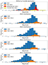 |
Fig. A.1. Distribution of different Spitzer bands for the SMC (blue) and NGC 6822 (orange). The red histogram shows the predicted MIPS [24] band and the yellow demonstrates the JWST [21] band. The values for NGC 6822 were corrected for the distance difference between the two galaxies. |
We derived the mass-loss rates and we present the results with respect to luminosity and the best-fit optical depth in Fig. A.2. In the cases where JWST mid-IR photometry existed, we did not use the ML [24] predicted values. Comparing Fig. A.2 with Fig. 6, we notice that a significant number of RSGs at 4 < log(L/L⊙) ≲ 4.7 have now lower Ṁ appearing as dust-free, but they agree within the errors. The more luminous RSGs almost agree and 4 RSGs that appeared as low Ṁ outliers in Fig. 6, now follow the rest of the distribution.
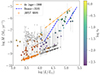 |
Fig. A.2. Same as Fig. 6 but using the ML predicted photometry for Spitzer [24] in the SED fitting procedure to derive the mass-loss rate. |
Finally, we examined the sample of RSGs presented in our previous study in the LMC (Antoniadis et al. 2024), to investigate if it is secure to use photometry at bands up to 8 μm, as we did in our main result for NGC 6822. To achieve this, we calculated the ratio of the derived Ṁ using photometry in all bands in the LMC over the Ṁ using photometry up to Spitzer [8.0]. We found that the two Ṁ agree within an order of magnitude for the majority of RSGs at log(L/L⊙) > 4. The median value of the ratio is 1.4 and the mean is 7.4, driven by some outliers. We demonstrate this result in Fig. A.3. Thus, there is more confidence in our derived Ṁ of RSGs in the NGC 6822 than our estimated errors presented in Fig. 6.
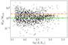 |
Fig. A.3. Ratio of the derived Ṁ using photometry in all bands over the derived Ṁ using photometry up to 8 μm for RSGs in the LMC. The green dashed line demonstrates the ratio of 1. The dotted and dot-dashed orange lines indicate the median (at 1.4) and mean for log(L/L⊙) > 4, respectively. |
Appendix B: M31 and M33
We computed the mass-loss rates of the RSG candidates in M31 and M33 from the sample of Wang et al. (2021). We show example SEDs of RSGs in M31 and M33 in Fig. B.1 and B.2, respectively. The Spitzer photometry indicates abnormally high infrared excess compared to the other galaxies at closer distance, especially at [24], which is also seen in the example SEDs (blending in Spitzer photometry for M33 was also found by Javadi et al. 2015). Correspondingly, Fig. B.3 and B.4 demonstrate the resulting Ṁ versus L in M31 and M33. It has to be mentioned that Wang et al. (2021) found higher Ṁ than our work. The main reason is that they assumed an MRN grain size distribution in the range of [0.01, 1] which would result in higher Ṁ by a factor of 20-30 (see Antoniadis et al. 2024) and used the relation for the outflow speed for the LMC from Goldman et al. (2017), which is steep and also results in higher Ṁ.
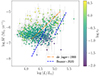 |
Fig. B.3. Mass-loss rate as a function of the luminosity of each RSG candidate in M31. The colour bar shows the best-fit τV. The lines are the same as in Fig. 6. |
Appendix C: RSG catalogues and results
Properties and derived parameters of the RSG candidates in the SMC.
Properties and derived parameters of the RSGs in the MW.
Properties and derived parameters of the RSG candidates in the NGC 6822.
Appendix D: Spectroscopic RSGs in the LMC and SMC
We used the spectroscopic RSGs from the LMC and SMC to determine whether there is a turning point in the Ṁ versus L relation. However, there are insufficient spectroscopic RSGs in the literature for the LMC at low L to determine a turning point. Figure D.1 shows the result from the LMC and our derived linear relation using Eq. 4.
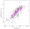 |
Fig. D.1. Mass-loss rates of RSGs in the LMC with spectroscopic classifications from the literature. Triangles indicate upper limits. The magenta points represent the prediction from fitted Ṁ(L,Teff) relation. |
The SMC has more data at low L than the LMC. Thus, we fitted both a linear relation and a broken law to examine which reproduces the measured Ṁ better. Table D.1 presents the best-fit coefficients of Eq. (4) for the spectroscopic RSGs in the LMC and SMC. Figure D.2 shows the derived linear relation and the residuals for the SMC, and Fig. D.3 the corresponding relation and residuals using a broken-law at log(L/L⊙) = 4.65. Finally, the upper limit for the fraction of dust-free spectroscopic RSGs in the SMC is 20%. We should note that the value of c2 for the SMC broken law for log(L/L⊙) = 4.65 is positive, not showing an anti-correlation with Teff, as we would expect, and with substantial error. This is probably because of the low number of spectroscopic RSGs at that range and should not be considered. We suggest using the relation assuming an average Teff or the derived Ṁ relation for the whole sample of RSGs in the SMC, presented in our main results.
Best-fit parameters of Eq. (4) for the spectroscopic RSGs in the LMC and SMC.
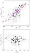 |
Fig. D.2. Top: Mass-loss rates of RSGs in the SMC with spectroscopic classifications from the literature. Triangles indicate upper limits. Bottom: Residual Ṁ values, defined as |

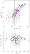 |
Fig. D.3. Top: Mass-loss rates of RSGs in the SMC with spectroscopic classifications from the literature. Triangles indicate upper limits. Bottom: Residual Ṁ values, defined as |

Appendix E: Mass-loss rates as a function of mid-infrared colours
Figure E.1 presents the mass-loss rates of RSGs with log(L/L⊙) > 4 as a function of different mid-IR colours (corrected for foreground extinction). We have shown that dust production is correlated with metallicity, which affects the mid-IR excess, and it is also known that the intrinsic colour of RSGs is metallicity dependent (e.g. Li et al. 2025). The dashed and dotted vertical lines in the top left panel of Fig. E.1 indicate the median values at Ṁ < 10−7 M⊙ yr−1 for the LMC and SMC, respectively, which differ by 0.07 mag. The turn at Ṁ > 10−7 M⊙ yr−1 becomes sharper at higher metallicity. The results from NGC 6822 are more dispersed due to the worse quality of Spitzer photometry at that distance but seem to agree with the SMC. This turn and the trend with metallicity is clearer in Fig. E.1 because the W3 band is connected with the silicate bump at around 10 μm. However, the open squares show the Ṁ of the Galactic RSGs with not well-fit near-IR photometry to the models, which could be underestimated, as we have mentioned.
The bottom right panel of Fig. E.1 shows the luminosity as a function of the Ks − W3 colour. According to Beasor & Smith (2022), Ks − W3 > 3.4 mag indicates candidate dust-enshrouded RSGs. These RSGs consist of roughly 0.6% of our total sample or RSGs with WISE3 photometry. We should mention that the samples of RSG candidates in the LMC and SMC could be biased against the inclusion of dust-enshrouded stars due to the photometric selection criteria. Nevertheless, we found a similar fraction considering only the Galactic RSGs. The sample may still not be complete, but it supports the argument from Beasor & Smith (2022) of the extreme scarcity of such RSGs.
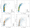 |
Fig. E.1. Top: Mass-loss rate as a function of colour for the LMC (blue), SMC (orange), and NGC 6822 (green triangles). The dashed and dotted vertical lines on the left panel indicate the median values at log(Ṁ/(M⊙ yr−1)) < −7 for the LMC and SMC, respectively. Bottom: Colour mass-loss rate (left) and colour luminosity (right) diagrams for the LMC (blue), SMC (orange), and MW (grey squares). The open squares indicate the more uncertain Ṁ in the MW with not well-fit JHKs photometry. The dashed vertical line shows the limit above which there are candidate dust-enshrouded RSGs. |
All Tables
All Figures
|
Fig. 1. HR diagram of the RSG samples in the LMC (blue circles), SMC (orange crosses), MW (black squares), and the NGC 6822 (green triangles). Four POSYDON evolutionary tracks for [Z]= − 0.7 and [Z] = 0 are shown in red and dotted dark red lines, respectively, and the points indicate intervals of 10 000 yr. The upper and right panels show the density histograms (areas equal to 1) of the effective temperature and luminosity, respectively. |
| In the text | |
|
Fig. 2. Examples of SED fits of SMC (top row), Galactic (middle), and NGC 6822 (bottom row) RSGs. The orange diamonds show the observations and the black line is the best-fit model consisting of the attenuated flux (dashed light blue), the scattered flux (dash-dotted grey), and dust emission (dotted brown). The top left corner includes the co-ordinates of each source in degrees. Notes: All SED fit figures are available in an electronic form via https://zenodo.org/records/16736627. |
| In the text | |
|
Fig. 3. Distribution of the minimum χmod2 for the LMC (blue bar), SMC (orange bar), MW (black line), and NGC 6822 (green line). The vertical dashed line indicates the considered limit for a good fit at χmod2 = 1.4. |
| In the text | |
|
Fig. 4. Distribution of the minimum τV for the RSGs in the LMC (blue bar), SMC (orange bar), MW (black line), and NGC 6822 (dashed green line). The dashed and dash-dotted histograms correspond to the RSGs in M31 and M33, respectively. |
| In the text | |
|
Fig. 5. Top: mass-loss rates vs. luminosity for SMC (left) and MW (right). The colour bar shows the Teff. The grey triangles represent the upper limits, and the open circles indicate the RSGs with spectral classifications. The magenta points correspond to the prediction of the derived Ṁ(L,Teff) relation. The dashed blue lines show the prescription from Beasor et al. (2020) for initial masses of 10 and 20 M⊙ and the dash-dotted orange line is the one from de Jager et al. (1988). Middle: MAD of W1 band vs luminosity diagram for the SMC (left) and the MW (right). The colour bar shows the mass-loss rate. Bottom: mass-loss rates vs the effective temperature for the SMC (left) and the MW (right) indicating the luminosity with colour. |
| In the text | |
|
Fig. 6. Derived mass-loss rate as a function of the luminosity of each RSG candidate in NGC 6822. The colour bar shows the best-fit τV. RSGs with spectral classifications are outlined in black. Orange circles denote the sources that have JWST MIRI photometry. Dashed blue lines show the prescription from Beasor et al. (2020) for initial masses of 10 and 20 M⊙; the dash-dotted orange line is from de Jager et al. (1988). |
| In the text | |
|
Fig. 7. Comparison of the mass-loss rates from all the galaxies studied: the LMC (blue circles), SMC (orange crosses), MW (black squares), and NGC 6822 (green triangles). The red points denote mass-loss rates derived from gas diagnostics. The solid lines show the prescription from Beasor et al. (2020) for initial masses of 10 and 20 M⊙, and the dash-dotted line is the relation from de Jager et al. (1988). The transparent symbols for MW and NGC 6822 indicate uncertain results. The shaded region includes stars with log(L/L⊙) < 4, which are less likely RSGs. |
| In the text | |
|
Fig. 8. Mass-loss rates of RSGs in the SMC with spectroscopic classifications from the literature. Triangles indicate upper limits and the colour indicates the effective temperature using Eq. (1). |
| In the text | |
|
Fig. 9. Median-absolute-deviation (MAD) diagram of W1 band of RSGs in the SMC with spectroscopic classifications from the literature. The colour indicates the corresponding mass-loss rates. The vertical dashed line shows the position of the kink from Fig. 5 at log(L/L⊙) = 4.65. |
| In the text | |
|
Fig. 10. Fraction of the Galactic RSGs from Healy et al. (2024) over the total number of K or M-type bright stars from their initial sample. |
| In the text | |
|
Fig. 11. Distribution of the mass-loss rate of RSGs with log(L/L⊙) > 4.5 for the LMC (blue bar), SMC (orange bar), MW (black line), and NGC 6822 (dashed green line). |
| In the text | |
|
Fig. 12. Median mass-loss rate vs. metallicity for each galaxy of our study and two luminosity ranges. |
| In the text | |
|
Fig. 13. Distribution of the dust-production rate of RSGs with log(L/L⊙) > 4 for the LMC (blue bar), SMC (orange bar), MW (black line), and NGC 6822 (dashed green line). |
| In the text | |
|
Fig. A.1. Distribution of different Spitzer bands for the SMC (blue) and NGC 6822 (orange). The red histogram shows the predicted MIPS [24] band and the yellow demonstrates the JWST [21] band. The values for NGC 6822 were corrected for the distance difference between the two galaxies. |
| In the text | |
|
Fig. A.2. Same as Fig. 6 but using the ML predicted photometry for Spitzer [24] in the SED fitting procedure to derive the mass-loss rate. |
| In the text | |
|
Fig. A.3. Ratio of the derived Ṁ using photometry in all bands over the derived Ṁ using photometry up to 8 μm for RSGs in the LMC. The green dashed line demonstrates the ratio of 1. The dotted and dot-dashed orange lines indicate the median (at 1.4) and mean for log(L/L⊙) > 4, respectively. |
| In the text | |
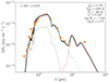 |
Fig. B.1. Example SEDs of two RSGs in M31. Symbols and lines are same as Fig. 2. |
| In the text | |
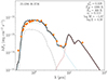 |
Fig. B.2. Example SEDs of two RSGs in M33. Symbols and lines are same as Fig. 2. |
| In the text | |
|
Fig. B.3. Mass-loss rate as a function of the luminosity of each RSG candidate in M31. The colour bar shows the best-fit τV. The lines are the same as in Fig. 6. |
| In the text | |
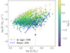 |
Fig. B.4. Same as Fig. B.3, but for M33. |
| In the text | |
|
Fig. D.1. Mass-loss rates of RSGs in the LMC with spectroscopic classifications from the literature. Triangles indicate upper limits. The magenta points represent the prediction from fitted Ṁ(L,Teff) relation. |
| In the text | |
|
Fig. D.2. Top: Mass-loss rates of RSGs in the SMC with spectroscopic classifications from the literature. Triangles indicate upper limits. Bottom: Residual Ṁ values, defined as |
| In the text | |
|
Fig. D.3. Top: Mass-loss rates of RSGs in the SMC with spectroscopic classifications from the literature. Triangles indicate upper limits. Bottom: Residual Ṁ values, defined as |
| In the text | |
|
Fig. E.1. Top: Mass-loss rate as a function of colour for the LMC (blue), SMC (orange), and NGC 6822 (green triangles). The dashed and dotted vertical lines on the left panel indicate the median values at log(Ṁ/(M⊙ yr−1)) < −7 for the LMC and SMC, respectively. Bottom: Colour mass-loss rate (left) and colour luminosity (right) diagrams for the LMC (blue), SMC (orange), and MW (grey squares). The open squares indicate the more uncertain Ṁ in the MW with not well-fit JHKs photometry. The dashed vertical line shows the limit above which there are candidate dust-enshrouded RSGs. |
| In the text | |
Current usage metrics show cumulative count of Article Views (full-text article views including HTML views, PDF and ePub downloads, according to the available data) and Abstracts Views on Vision4Press platform.
Data correspond to usage on the plateform after 2015. The current usage metrics is available 48-96 hours after online publication and is updated daily on week days.
Initial download of the metrics may take a while.