| Issue |
A&A
Volume 702, October 2025
|
|
|---|---|---|
| Article Number | A29 | |
| Number of page(s) | 8 | |
| Section | Stellar structure and evolution | |
| DOI | https://doi.org/10.1051/0004-6361/202554548 | |
| Published online | 29 September 2025 | |
NLTE spectral modelling for a carbon-oxygen and helium white dwarf merger as a Ca-rich transient candidate
1
School of Mathematics and Physics, Queen’s University Belfast, University Road, Belfast BT7 1NN, UK
2
Heidelberger Institut für Theoretische Studien, Schloss-Wolfsbrunnenweg 35, D-69118 Heidelberg, Germany
3
Cosmic Dawn Center (DAWN), Denmark
4
Niels Bohr Institute, University of Copenhagen, Jagtvej 155A, DK-2200 Copenhagen N, Denmark
5
School of Physics, Trinity College Dublin, The University of Dublin, Dublin 2, Ireland
6
GSI Helmholtzzentrum für Schwerionenforschung, Planckstraße 1, 64291 Darmstadt, Germany
7
Zentrum für Astronomie der Universität Heidelberg, Astronomisches Rechen-Institut, Mönchhofstraße 12–14, 69120 Heidelberg, Germany
8
Zentrum für Astronomie der Universität Heidelberg, Institut für Theoretische Astrophysik, Philosophenweg 12, 69120 Heidelberg, Germany
9
Max-Planck-Institut für Astrophysik, Karl-Schwarzschild-Str. 1, D-85748 Garching, Germany
⋆ Corresponding author: This email address is being protected from spambots. You need JavaScript enabled to view it.
Received:
14
March
2025
Accepted:
27
July
2025
Abstract
We carried out NLTE (non local thermodynamic equilibrium) radiative transfer simulations to determine whether an explosion during the merger of a carbon-oxygen (CO) white dwarf (WD) with a helium (He) WD can reproduce the characteristic Ca II/[Ca II] and He I lines observed in Ca-rich transients. Our study is based on a 1D representation of a hydrodynamic simulation of a 0.6 M⊙ CO+0.4 M⊙ He WD merger. We calculated both the photospheric and nebular-phase spectra, including treatment for non-thermal electrons, as is required for accurate modelling of He I and [Ca II]. Consistent with Ca-rich transients, our simulation predicts a nebular spectrum dominated by emission from [Ca II] 7291, 7324 Å and the Ca II near-infrared (NIR) triplet. The photospheric-phase synthetic spectrum also exhibits a strong Ca II NIR triplet, prominent optical absorption due to He I 5876 Å and He I 10830 Å in the NIR, which is commonly observed for Ca-rich transients. Overall, our results therefore suggest that CO+He WD mergers are a promising channel for Ca-rich transients. However, the current simulation overpredicts some He I features, in particular both He I 6678 and 7065 Å, and shows a significant contribution from Ti II, which results in a spectral energy distribution that is substantially redder than most Ca-rich transients at peak. Additionally, the Ca II nebular emission features are too broad. Future work should investigate if these discrepancies can be resolved by considering full 3D models and exploring a range of CO+He WD binary configurations.
Key words: radiative transfer / methods: numerical / supernovae: general / white dwarfs
© The Authors 2025
 Open Access article, published by EDP Sciences, under the terms of the Creative Commons Attribution License (https://creativecommons.org/licenses/by/4.0), which permits unrestricted use, distribution, and reproduction in any medium, provided the original work is properly cited.
This article is published in open access under the Subscribe to Open model. This email address is being protected from spambots. You need JavaScript enabled to view it. to support open access publication.
1. Introduction
Ca-rich transients (see e.g. Taubenberger 2017 for a review) are a class of faint and fast-evolving supernovae (SNe) first observed in the early 2000s (Filippenko et al. 2003). They are primarily characterised by strong [Ca II] emission and weaker [O I] emission in their nebular spectra1 (Perets et al. 2010; Sullivan et al. 2011; Kasliwal et al. 2012; Valenti et al. 2014; Lunnan et al. 2017; De et al. 2018). Other properties include peak luminosities that lie between those of novae and SNe (∼ − 14 to −17 mag), fast photometric evolution, and early evolution to the nebular phase (Kasliwal et al. 2012). The spectroscopic properties of Ca-rich transients are diverse, with some more similar to Type Ia SNe and others more similar to Type Ibc SNe (De et al. 2020).
The progenitors of Ca-rich transients are still unknown. However, the fact that they are typically found in remote locations in old host environments (Perets et al. 2010; Foley 2015; Lunnan et al. 2017) suggests older progenitors that involve white dwarfs (WDs) in binary systems. Various models have been proposed to explain Ca-rich transients, including helium (He) shell detonations (e.g. Perets et al. 2010; Shen et al. 2010; Waldman et al. 2011; Woosley & Kasen 2011), tidal disruptions of WDs either in a compact object binary (e.g. Margalit & Metzger 2016; Zenati et al. 2023) or by an intermediate-mass black hole (e.g. Rosswog et al. 2009; Sell et al. 2015), and ultra-stripped core-collapse SNe (e.g. Kawabata et al. 2010; see e.g. Shen et al. 2019 for a review).
In a previous work we presented a 3D hydrodynamic simulation of the merger of a 0.4 M⊙ He WD and a 0.6 M⊙ carbon-oxygen (CO) WD (Morán-Fraile et al. 2024). During the merger, the He WD is tidally disrupted and the CO WD becomes engulfed in a massive He ‘shell’. As the orbit of the accreting material intersects with itself, efficiently transporting angular momentum outwards, a region that is overdense relative to the surrounding gas develops. Compression and shear between this overdense region and the surface of the CO WD result in a He detonation ∼400 s after the He WD was initially disrupted. The detonation wave propagates through the He shell that surrounds the CO WD, sending shocks inside it. The convergence of these shocks ignites a C detonation that propagates outwards and burns the CO material. Overall, the thermonuclear explosion resulting from this double detonation mechanism ejected 1 M⊙ of material, synthesised 0.01 M⊙ of 56Ni, and did not leave behind any remnant. Photospheric phase radiative transfer simulations of the model predicted a faint transient (Mbol ≈ −15.7) with light curves and spectra that resembled those of Ca-rich transients, including a prominent Ca II near-infrared (NIR) triplet feature, as is observed in the photospheric spectra of such events. This suggests that such mergers are a possible progenitor system of Ca-rich transients.
However, open questions remain. The Morán-Fraile et al. (2024) radiative transfer simulation was unable to reproduce the strong feature around 5900 Å that is observed in the majority of Ca-rich transients, interpreted as either the He I 5876 Å line or the Na I 5890, 5896 Å doublet (Na I D). The lack of He features predicted, despite the significant He mass in the model ejecta (0.3 M⊙), was not unexpected, as the radiative transfer simulation utilised an approximate NLTE (non local thermodynamic equilibrium) treatment for the plasma conditions that did not include treatment for non-thermal electrons. As the temperatures of the ejecta of thermonuclear SNe are insufficient to thermally excite He I, it is these non-thermal electrons that dominate the population of the excited states of He I such that spectral features can appear (Chugai 1987; Lucy 1991; Hachinger et al. 2012). The approximate NLTE treatment of the plasma conditions also means the simulation becomes increasingly unreliable beyond the photospheric phase. As such, no predictions of the nebular phase spectra, by which Ca-rich transients are most readily identified, were possible from that simulation.
Here, we present full NLTE photospheric and nebular phase radiative transfer simulations, including treatment for non-thermal electrons, for a 1D spherical average of the 0.6 M⊙ CO+0.4 M⊙ He WD merger model. In particular, our aim is to predict whether He I lines form in the photospheric phase and if the nebular spectra display the prominent Ca II emission observed for Ca-rich transients. We describe our model ejecta structure and our radiative transfer setups for the photospheric and nebular phase simulations in Sect. 2. We present our photospheric and nebular phase spectra in Sect. 3 before discussing the model predictions and comparing them with observed Ca-rich transients in Sect. 4. Finally, we present our conclusions in Sect. 5.
2. Numerical methods
2.1. NLTE and non-thermal radiative transfer
The radiative transfer simulations are carried out using the time-dependent Monte Carlo radiative transfer code ARTIS2 (Sim 2007; Kromer & Sim 2009; Bulla et al. 2015; Shingles et al. 2020). ARTIS follows the methods of Lucy (2002, 2003, 2005) and is based on dividing the radiation field into indivisible energy packet Monte Carlo quanta (packets hereafter). Here, we utilise the full NLTE and non-thermal capabilities added to ARTIS by Shingles et al. (2020). This includes a NLTE population and ionisation solver and treatment for collisions with non-thermal leptons. These improvements both extend the validity of our radiative transfer simulations to the nebular phase and allow the spectral contribution of He to be predicted. To follow the energy distribution of high-energy leptons, which result from nuclear decays and Compton scattering of γ-rays, ARTIS solves the Spencer-Fano equation (as framed by Kozma & Fransson 1992). Auger electrons are allowed to contribute to heating, the ionisation and excitation of bound electrons by non-thermal collisions is also included. ARTIS utilises the full Monte Carlo photon-packet trajectories to obtain a rate estimator for each photoionisation cross-section included while a parameterised radiation field is used to estimate bound-bound transition rates. The atomic datasets we use are based on the compilation of CMFGEN (Hillier 1990; Hillier & Miller 1998) and are similar to that described by Shingles et al. (2020) but with some additional species and ions including atomic data for Ca IV, Ti II, Ti III, Co I and Ni I from the most recent compilation of CMFGEN (see Blondin et al. 2023). In our photospheric phase simulation we include He I-III, C I-IV, O I-IV, Na I-III, Ne I-III, Mg I-III, Al I-IV, Si I-IV, S I-IV, Ar I-IV, Ca I-V, Ti II-IV, Cr I-V, Fe I-V, Co II-V, and Ni II-V, while we also include Co I and Ni I in our nebular phase simulation. We note that there is no Ti I data in our atomic dataset. We do not expect Ti I to become the dominant ion in our simulations (we do include both Ca I and Cr I, which remain subdominant ions at all times). However, it is possible that Ti I could contribute to the spectrum in the later phases we consider when the temperature and ionisation state are low. However, we do not expect that this would significantly impact our principle conclusions on the formation of He I and Ca II features.
To cover both the photospheric and nebular phases, we performed two separate simulations because a significantly greater number of packets are required when simulating the nebular phase (a factor of ∼40; see below). This is because we start with the packets representing gamma-rays and positrons arising from radioactive decays (Kromer & Sim 2009). During the simulation these packets can be reprocessed to UVOIR wavelengths from which we ultimately extract the spectra. Owing to the optically thin conditions in the nebular phase, the fraction of the gamma-ray packets that are reprocessed is much smaller, meaning we require a much larger total number of packets in order to achieve good statistics in the required wavebands. Fortunately however, the number of interactions per packets in this optically thin regime is relatively small, meaning this increase in total number of packets does not present a computational problem.
We utilised 5 × 10⁷ packets for the photospheric phase simulation, which describes the evolution from 1 to 40 d post explosion with logarithmically spaced time steps (Δlog(t) = 0.013). The initial time steps were treated in local thermodynamic equilibrium (LTE) and at time step 12 (1.1 d) the NLTE solver was switched on. We adopted a grey approximation in optically thick cells (those with a grey optical depth greater than 1000).
We initialised the nebular phase simulation at 25 d post explosion and followed the spectroscopic evolution using 2 × 10⁹ packets until 70 d post explosion with logarithmically spaced time steps (Δlog(t) = 0.0037). The initial time steps of the nebular phase simulation were also treated in LTE and the NLTE solver was switched on at time step 12 (28 d).
2.2. CO He WD merger ejecta model
For this work, we utilised the WD merger model of Morán-Fraile et al. (2024), who simulated the merger of a 0.4 M⊙ He WD and a 0.6 M⊙ CO WD. This simulation was carried out using the AREPO code (Springel 2010; Pakmor et al. 2011, 2016; Weinberger et al. 2020), which solves the ideal magnetohydrodynamic equations on an unstructured moving Voronoi mesh using Newtonian self-gravity, including a Helmholtz equation of state Timmes & Swesty (2000). A 55 isotope nuclear reaction network, using the JINA reaction rates Cyburt et al. (2010) was coupled to the hydrodynamical solver. The simulation was stopped when the ejecta reaches homologous expansion, around 100 s after the explosion takes place. Using a larger 384 isotope network, the 106 Lagrangian tracer particles included in the simulation were post-processed to obtain precise nucleosynthetic yields (Seitenzahl et al. 2010; Pakmor et al. 2012; Seitenzahl & Townsley 2017). For further details on the model, we refer the reader to Morán-Fraile et al. (2024).
While ARTIS is capable of multi-dimensional simulations, owing to the increased computational cost of including our full NLTE treatment, we worked in 1D for this first exploratory study and employed a spherically averaged model. The full 3D model has clear asymmetries (see Morán-Fraile et al. 2024 or Kozyreva et al. 2024) that likely impact the strengths and shapes of spectral features. However, the 1D average preserves the main characteristics of the model, which allowed us to address the key questions of whether He I and [Ca II] line formation are plausible. We constructed our 1D model by spherically averaging the 3D hydrodynamic simulation into 87 radial bins. The composition of this 1D ejecta model is presented in Table 1 and shown in Fig. 1 along with the energy deposition profiles at the epochs we present spectra for. From Fig. 1 we can see that because the He distribution extends to low velocities there is significant overlap between where the He is present in the ejecta and where the deposition is taking place.
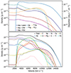 |
Fig. 1. Bottom panel: model ejecta composition at 160 s after explosion for key species in the simulation. Top panel: energy deposition profiles for the three epochs we show spectra for. Overplotted for reference are the density profiles of He and key radioisotopes that we track the decay chain energy deposition for in the simulation. |
Compositions of key species in our radiative transfer input model (in solar masses) at 160 s post explosion.
3. Results
Figures 2 and 3 show the optical and NIR spectra predicted by our simulations. We display three epochs with the r-max and +20 d r-max spectra taken from our photospheric phase simulation and the +45 d r-max spectrum taken from our nebular phase simulation3.
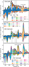 |
Fig. 2. Optical spectroscopic evolution of our model from peak until the early nebular phase. The last species with which packets interacted before they left the simulation are indicated with different colours. Contributions to emission are plotted on the positive axis, and contributions to absorption on the negative axis. For reference, key lines are labelled along with their rest wavelength (given in Å). The dashed lines indicate the wavelengths of absorptions from the prominent optical He I lines. |
3.1. Optical spectroscopic evolution
The peak r-band optical spectrum of our simulation (see Fig. 2) predicts strong optical He I features (He I 5876, 6678 and 7065 Å) with He I 5876 Å producing the strongest feature. This is a key difference to our previous radiative transfer simulation of the model (Morán-Fraile et al. 2024), which did not include treatment for non-thermal electrons and thus could not address whether He I spectral features are expected to form.
The Ca II NIR triplet, which appears around 8300 Å, is the strongest individual feature in the peak spectrum. Additionally, there is a very significant contribution from Ti II and Cr II that covers almost the entire optical wavelength range. The substantial absorption, in particular from Ti II, bluewards of ∼5000 Å and subsequent redistribution of this flux to redder wavelengths results in a relatively red spectral energy distribution (SED) at peak. There is a clear contribution from the O I 7773 Å line at peak along with small contributions from intermediate-mass elements such as Si and S. Only very weak contributions from iron group elements are predicted.
At 20 d post r-band peak, our simulation is already starting to show signs of a transition to the nebular phase with strong emission features typically associated with nebular phase spectra beginning to form. The spectrum still shows a very substantial contribution from Ti II while the spectral contribution of Cr II is significantly reduced. There is almost a complete suppression of flux bluewards of ∼5000 Å due to line blanketing primarily from Ti II. The Ca II NIR triplet remains the strongest individual feature at this epoch showing very substantial emission. The simulation also predicts a strong emission feature around 7300 Å. Although this feature appears to be almost entirely dominated by Ti II 7355 Å with a small contribution to emission from forbidden [Ca II] 7291, 7324 Å (see Fig. 2), a significant amount of the underlying emission is actually attributed to [Ca II] with this emission then impacted by scattering and fluorescence from the Ti II 7355 Å line.
The optical He I features predicted in the peak spectrum are again present although the strength of the He I lines are reduced relative to peak. In particular, the strong feature at ∼5700 Å that is almost entirely a result of He I 5876 Å absorption in the peak spectrum is now a blend of He I 5876 Å and Na I D lines with Na I contributing strongly to the formation of this feature, particularly in emission. This can primarily be attributed to variation in the ionisation state of Na. At peak, less than 10−6 of the total Na in the ejecta is Na I. However, by 20 d post peak this has increased to as much as 10−3 in certain parts of the model ejecta. Variation in the distribution of Na in our model ejecta (see Fig. 1) may also be contributing, with Na only present in very small amounts in the very outer and inner ejecta but showing a significant increase in relative composition between ∼3000 and 10 000 km s−1. As the photosphere recedes deeper into the ejecta with time, the spectrum forming region therefore evolves to overlap with this part of the ejecta that is richer in Na. There remains a relatively strong contribution from O I 7773 Å at 20 d post peak while there are still clear contributions from intermediate-mass elements and only weak contributions from iron group elements to the model spectrum.
By 45 d post peak, our simulated optical spectrum becomes dominated by emission redwards of 6000 Å although there is still significant absorption, particulary bluewards of this, mainly due to Ti II and Fe I. The most prominent spectral features are the Ca II NIR triplet and the forbidden [Ca II] 7291, 7324 Å emission feature, which appear around 8700 and 7300 Å, respectively. While the majority of the underlying emission for these features is from Ca II and [Ca II] respectively, both features are still clearly impacted by scattering and fluorescence from allowed transitions (primarily Fe I, TiII, and Mg I for the NIR triplet and Ti II and Ca I for the [Ca II] feature).
Ti II remains a key species in the spectrum, contributing significantly across a range of wavelengths spanning the entire optical spectrum. There is a significant increase in the contributions of neutral species such as Fe I, Ca I, Cr I, SiI, and Co I. This is a result of the reduced ionisation state of the simulation at this epoch. In particular, Fe I has a substantial contribution across a wide range of optical wavelengths and the Fe I feature predicted at ∼5500 Å, which also has contributions from Co I and Ni I, is the most prominent feature in the spectrum other than the Ca II/[Ca II] features discussed above. The complex of emission features predicted by the simulation between ∼6000 and 7000 Å is also primarily attributed to the blended contributions of neutral species (Fe I, Ca I, Cr I, and Co I).
3.2. NIR spectroscopic evolution
The most prominent feature in the peak NIR spectrum predicted by our simulation is the strong He I 10 830 Å absorption feature (see Fig. 3), while there is also a clear He I 20 587 Å absorption feature. We note that substantial ejected He masses, such as the ∼0.3 M⊙ ejected for our model, are likely required for a He I 20587 Å feature to appear: previous ARTIS simulations of CO WD explosions, ejecting ∼0.04 M⊙ of He, predicted clear He I 10 830 Å features, but no obvious He I 20 587 Å feature formed (Collins et al. 2023; Callan et al. 2025). A prominent Ca II 11 839, 11 950 Å absorption feature is also present at ∼11 500 Å. The NIR spectrum is dominated by Ti II emission for wavelengths shorter than ∼16 000 Å while redwards of this He I provides the greatest contribution to the spectrum.
At 20 days post peak, the NIR spectrum starts to show emission features more typical of the nebular phase. He I 10 830 Å remains the strongest spectral feature predicted by the simulation in the NIR and the He I 20 587 Å feature is still clearly present. The Ca II absorption at ∼11 500 Å has disappeared by this epoch but there is still significant emission from Ti II. There is also an increased contribution from neutral species, in particular Si I and Ca I.
At 45 d post peak, clear He I 10 830 and 20 587 Å features are still predicted despite no optical He features being present in the simulation by this epoch. The single strongest feature at this epoch is the strong emission feature at ∼12 000 Å. This feature is primarily attributed to Fe I but there is a also a contribution from Si I. A prominent Al I feature also appears at ∼13 500 Å.
We note, for the small number of Ca-rich transients that have NIR spectral observations, a clear feature is present at wavelengths consistent with our predicted He I 10 830 Å feature (Valenti et al. 2014; Galbany et al. 2019; Jacobson-Galán et al. 2020a; Yadavalli et al. 2024) for observations spanning from before peak until 40 d post peak. Additionally, the Ca-rich transient SN 2019ehk (Jacobson-Galán et al. 2020a) shows a feature consistent with the predicted He I 20 587 Å feature.
4. Comparison to observations
We now present spectral comparisons with observed Ca-rich transients focusing on the key Ca II and He I features. Given that we are only comparing the observations to a single 1D model, and that there is substantial spectral diversity displayed by Ca-rich transients (see e.g. De et al. 2020), we cannot expect our current model to fully account for all features in the observations, or explain their variations. In the following we show, however, that our simulations do predict the Ca II/[Ca II] and He I features, which are characteristic of Ca-rich transients.
4.1. Model comparisons with observations at peak
As can be seen from Fig. 4 there are very few spectral features at peak that are consistently present in the spectra of observed Ca-rich transients. There are, however, two features that are effectively ubiquitous in their peak optical spectra: the Ca II NIR triplet and the absorption feature attributed to either the He I 5876 Å or Na I D lines. Our simulation predicts a Ca II NIR triplet at peak with a strength and velocity generally consistent with that observed in the spectra of Ca-rich transients (although, as expected, there is variation in the quality of agreement depending on which Ca-rich transient we compare with). A clear He I 5876 Å feature is also predicted, which has a strength comparable to the observed feature present around 5700 Å and also has a velocity that is in most cases consistent with that of the observed feature (but we note the deepest absorption of the predicted feature is at too high a velocity compared to the feature observed for SN 2019ehk).
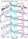 |
Fig. 4. Spectroscopic comparisons around peak of our simulated spectra with the observed Ca-rich transients SN 2012hn (Valenti et al. 2014), SN 2019ehk (Jacobson-Galán et al. 2020b; Nakaoka et al. 2021), SN 2010et (Kasliwal et al. 2012), SN PTF11kmb (Lunnan et al. 2017), and SN iPTF16hgs (De et al. 2018). The model epochs are relative to the Sloan r-band peak and have been chosen to match the epochs of each observed spectrum relative to either the Sloan r-band or the Bessel R-band peak. For reference, the strong optical He I features, attributed to the He I 5876, 6678, and 7065 Å lines, are highlighted in cyan and the Ca II NIR triplet is highlighted in pink. |
Our simulation predicts He I 6678 and 7065 Å absorption features that are noticeably stronger than features at corresponding wavelengths in the observed Ca-rich transients we compare to in Fig. 4, with the exception of SN PTF11kmb. The SED at peak predicted by our simulation is noticeably redder than the Ca-rich transients we compare to, other than SN 2012hn. As noted above, the red SED of our simulation is a result of significant absorption by Ti II at wavelengths bluer than ∼5000 Å and subsequent redistribution of this flux to redder wavelengths. The impact of Ti II in the spectra of Ca-rich transients shows substantial variation (see e.g. De et al. 2020) with some events showing very little evidence of Ti II at peak while others show the same clear Ti II absorption trough at ∼4300 Å predicted by our simulation (see Fig. 4). The Ti in our simulation is produced almost entirely in the He detonation. Therefore, although there are some Ca-rich transients with comparable He I 6678 and 7065 Å line strengths and similarly red SEDs to our model, it is likely that the He (and Ti) mass of the model we investigate here is towards the high end of what would be expected for Ca-rich transients. We do however note that the He and Ti distributions vary strongly for different lines of sight as the ejecta show significantly asymmetric structures (see e.g. Kozyreva et al. 2024 Figures 3 and 4). Such viewing angle effects are not captured by the spherically averaged model investigated here. Additionally, the strength of the He and Ti features can be impacted by factors relevant to their ionisation state such as the distribution of 56Ni in the ejecta, which also varies significantly with viewing angle in the 3D ejecta model. As such, future work is required to investigate whether different lines of sight in the 3D ejecta model can explain the variation in optical He I and Ti II line strengths displayed by Ca-rich transients.
4.2. Model comparisons with observations in the nebular phase
As can be seen from Fig. 5, the nebular phase spectrum predicted by our simulation is dominated by the strong [Ca II] and Ca II emission features at around 7300 and 8700 Å, respectively. The simulated features have comparable strengths and velocities to the features observed in the nebular phase spectra of Ca-rich transients. However, our simulation predicts the Ca II NIR triplet emission to be stronger than the [Ca II] 7291, 7324 Å emission while these features have roughly equivalent strengths in the observed spectra4. Additionally, while we note the observed Ca II emission features show clear variations in their widths and velocities between different Ca-rich transients (see Fig. 5), our simulation predicts Ca II features that are too broad relative to the observations.
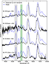 |
Fig. 5. Nebular phase spectroscopic comparisons of our simulated spectra at 45 d post r-band peak and the observed Ca-rich transients SN 2021gno (Jacobson-Galán et al. 2022; Ertini et al. 2023), SN 2022oqm (Yadavalli et al. 2024), SN 2019ehk (Jacobson-Galán et al. 2020b; Nakaoka et al. 2021), and SN PTF12bho (Lunnan et al. 2017) at similar epochs. The epochs of the observations are relative to the Sloan r-band or Bessel R-band peak. For reference, the dashed grey line is plotted between the rest wavelengths of the key [Ca II] 7291, 7324 Å lines, the Fe I emission feature predicted by the simulation is highlighted in grey, and the location of the [O I] 6300, 6364 Å feature commonly observed for Ca-rich transients is highlighted in green. |
From Fig. 5 we can see that the [Ca II] emission feature shows at least some level of asymmetry for all the observed Ca-rich transients and in the case of SN 2022oqm even appears to show a blue shift. This suggests multi-dimensional structures are present in these observations. However, we note our 1D simulation also appears to show a blue shift in the [Ca II] feature but this is actually attributed to the feature being partially blended with Ti II and Ca I. Future 3D radiative transfer simulations should therefore be carried out in order to investigate how the widths, velocity shifts and shapes of the Ca II features vary with viewing angle.
Bluewards of 7000 Å the observed Ca-rich transients show very substantial variation in their nebular phase spectra and as such the model has varying success in matching the observed spectra over this wavelength range. One feature that appears to be common to all the observations that we compare with here is the emission feature around 5500 Å, which the model attributes primarily to Fe I emission. Other than SN 2022oqm, all the Ca-rich transients which we compare to have an emission feature around 6300 Å attributed to [O I] 6300, 6364 Å. However, while the simulation predicts such an emission feature, the contribution of [O I] 6300, 6364 Å is quite minimal, with blended emission from a variety of species including Fe I, Cr I, Ca I, and Co I driving the formation of the feature (see Fig. 2). While this suggests the [O I] 6300, 6364 Å feature is not a clean diagnostic at this epoch, it will become more reliable at later times as forbidden emission increasingly dominates over the contribution of allowed transitions to the spectrum.
5. Conclusions
We have carried out 1D NLTE radiative transfer simulations, including treatment for non-thermal electrons, covering the photospheric and nebular phase for the merger of a 0.6 M⊙ CO+0.4 M⊙ He WD. Our aim was to establish whether the He I and Ca II/[Ca II] features characteristic of Ca-rich transients are predicted, and we find that they are. In particular, the simulation yields (i) a nebular spectrum dominated by emission from [Ca II] 7291, 7324 Å and the Ca II NIR triplet, and (ii) a peak spectrum that exhibits a strong Ca II NIR triplet and a prominent absorption feature at ∼5700 Å attributed to He I 5876 Å in our simulation.
Our simulation also predicts clear He I 10 830 and 20 587 Å features, which provide the best diagnostic of He in the model: in contrast to the optical He features, they are present at all epochs simulated and persist into the nebular phase. Although there are relatively few NIR observations of Ca-rich transients, existing observations do display a prominent feature at wavelengths similar to our predicted He I 10 830 Å feature (Valenti et al. 2014; Galbany et al. 2019; Jacobson-Galán et al. 2020a; Yadavalli et al. 2024) for observations spanning from before peak until 40 d post peak and SN 2019ehk also shows the He I 20 587 Å feature (Jacobson-Galán et al. 2020a).
Therefore, we conclude that low-mass CO WD + He WD mergers are promising Ca-rich transient candidates. However, it is not yet clear whether such models can account for the full range of observed objects in this class of transients. Our model shows a strong spectral contribution from Ti II at all epochs resulting in an SED at peak that is substantially redder than the majority of Ca-rich transients. The strong [Ca II]/Ca II emission features that dominate our simulated nebular spectra are too broad relative to observations, and the He I 6678, 7065 Å absorption features predicted at peak appear to be more prominent than in the majority of Ca-rich transients. Interestingly the simulations presented by Zenati et al. (2023) for a CO WD disrupted by a hybrid HeCO WD also produce nebular spectra with strong [Ca II] but in contrast do not display any strong contributions from He. Therefore, taken together, these different WD mergers can produce a family of transients that are unified by strong [Ca II] in their nebular spectra but show substantial variation in the strength of He spectral features predicted.
Future work should investigate whether the discrepancies between our model and observations can be resolved. In particular, the He and Ti distributions vary significantly with the line of sight in the 3D hydrodynamic merger simulation, suggesting that observer orientation may be important. The strength of He and Ti features can also be impacted by factors relevant to their ionisation state such as the distribution of 56Ni in the ejecta, which also shows significant variation with viewing angle in the 3D ejecta model. Additionally, the [Ca II] feature can show asymmetric profiles and, in some cases, blue shifts for observed Ca-rich transients, which may indicate that a multi-dimensional structure is present. Future multi-dimensional NLTE radiative transfer simulations should therefore be carried out to investigate if variation between lines of sight in the 3D ejecta model can better capture the variety observed for the Ca-rich class.
Ca-rich transients show a variation of approximately three magnitudes in peak r-band brightness. Therefore, further hydrodynamic merger simulations should be carried out to explore if systems with different combinations of CO and He WD masses can robustly explode and result in a diversity in peak brightness that can cover the variation observed for the Ca-rich class. Additionally, if systems with a lower mass He WD can explode, this should result in a reduction in the He and Ti ejected in the explosion. Future simultaneous optical and NIR observations (e.g. from SOXS; Schipani et al. 2018) will be ideal for the testing of such models as they will be able to capture both the overall SED and the key He I NIR features.
A substantial amount of Ca is not necessarily required to excite the nebular Ca II lines (Shen et al. 2019; Jacobson-Galán et al. 2020b; Polin et al. 2019). However, we use ‘Ca-rich’ throughout as it is the term that appears most commonly in the literature.
The spectra presented here will be made available on the Heidelberg supernova model archive HESMA (Kromer et al. 2017, https://hesma.h-its.org)
Radiative excitation still plays a role in the simulation at this time, which keeps the NIR triplet relatively strong.
Acknowledgments
FPC and SAS would like to acknowledge support from the UK Science and Technology Facilities Council (STFC, grant number ST/X00094X/1). This work used the DiRAC Memory Intensive service (Cosma8) at Durham University, managed by the Institute for Computational Cosmology on behalf of the STFC DiRAC HPC Facility (https://www.dirac.ac.uk/). The DiRAC service at Durham was funded by BEIS, UKRI and STFC capital funding, Durham University and STFC operations grants. DiRAC is part of the UKRI Digital Research Infrastructure. The authors gratefully acknowledge the Gauss Centre for Supercomputing e.V. (https://www.gauss-centre.eu/) for funding this project by providing computing time through the John von Neumann Institute for Computing (NIC) on the GCS Supercomputer JUWELS at Jülich Supercomputing Centre (JSC). AH is a fellow of the International Max Planck Research School for Astronomy and Cosmic Physics at the University of Heidelberg (IMPRS-HD) and acknowledges financial support from IMPRS-HD. This work has received funding from the European Union’s Horizon Europe research and innovation programme under the Marie Skłodowska-Curie grant agreement No. 101152610. LJS acknowledges support by the European Research Council (ERC) under the European Union’s Horizon 2020 research and innovation program (ERC Advanced Grant KILONOVA No. 885281). JMP acknowledges the support of the Department for Economy (DfE). This work received support from the European Research Council (ERC) under the European Union’s Horizon 2020 research and innovation programme under grant agreement No. 759253 and 945806, the Klaus Tschira Foundation, and the High Performance and Cloud Computing Group at the Zentrum für Datenverarbeitung of the University of Tübingen, the state of Baden-Württemberg through bwHPC and the German Research Foundation (DFG) through grant no INST 37/935-1 FUGG. The authors acknowledge support by the state of Baden-Württemberg through bwHPC and the German Research Foundation (DFG) through grant INST 35/1597-1 FUGG. This work was supported by the Deutsche Forschungsgemeinschaft (DFG, German Research Foundation) – RO 3676/7-1, project number 537700965, and by the European Union (ERC, ExCEED, project number 101096243). Views and opinions expressed are, however, those of the authors only and do not necessarily reflect those of the European Union or the European Research Council Executive Agency. Neither the European Union nor the granting authority can be held responsible for them. SAS thanks the Cosmic Dawn Center / Niels Bohr Institute (University of Copenhagen) who hosted his sabbatical visit during which part of this work was carried out. NumPy and SciPy (Oliphant 2007), Matplotlib (Hunter 2007) and ARTISTOOLS (https://github.com/artis-mcrt/artistools/) (Shingles et al. 2025) were used for data processing and plotting.
References
- Blondin, S., Dessart, L., Hillier, D. J., Ramsbottom, C. A., & Storey, P. J. 2023, A&A, 678, A170 [NASA ADS] [CrossRef] [EDP Sciences] [Google Scholar]
- Bulla, M., Sim, S. A., & Kromer, M. 2015, MNRAS, 450, 967 [Google Scholar]
- Callan, F. P., Collins, C. E., Sim, S. A., et al. 2025, MNRAS, 539, 1404 [Google Scholar]
- Chugai, N. N. 1987, Sov. Astron. Lett., 13, 282 [NASA ADS] [Google Scholar]
- Collins, C. E., Sim, S. A., Shingles, L. J., et al. 2023, MNRAS, 524, 4447 [Google Scholar]
- Cyburt, R. H., Amthor, A. M., Ferguson, R., et al. 2010, ApJS, 189, 240 [NASA ADS] [CrossRef] [Google Scholar]
- De, K., Kasliwal, M. M., Cantwell, T., et al. 2018, ApJ, 866, 72 [NASA ADS] [CrossRef] [Google Scholar]
- De, K., Kasliwal, M. M., Tzanidakis, A., et al. 2020, ApJ, 905, 58 [NASA ADS] [CrossRef] [Google Scholar]
- Ertini, K., Folatelli, G., Martinez, L., et al. 2023, MNRAS, 526, 279 [NASA ADS] [CrossRef] [Google Scholar]
- Filippenko, A. V., Chornock, R., Swift, B., et al. 2003, IAU Circ., 8159, 2 [NASA ADS] [Google Scholar]
- Foley, R. J. 2015, MNRAS, 452, 2463 [Google Scholar]
- Galbany, L., Ashall, C., Höflich, P., et al. 2019, A&A, 630, A76 [NASA ADS] [CrossRef] [EDP Sciences] [Google Scholar]
- Hachinger, S., Mazzali, P. A., Taubenberger, S., et al. 2012, MNRAS, 422, 70 [NASA ADS] [CrossRef] [Google Scholar]
- Hillier, D. J. 1990, A&A, 231, 116 [NASA ADS] [Google Scholar]
- Hillier, D. J., & Miller, D. L. 1998, ApJ, 496, 407 [NASA ADS] [CrossRef] [Google Scholar]
- Hunter, J. D. 2007, Comput. Sci. Eng., 9, 90 [NASA ADS] [CrossRef] [Google Scholar]
- Jacobson-Galán, W. V., Margutti, R., Kilpatrick, C. D., et al. 2020a, ApJ, 898, 166 [CrossRef] [Google Scholar]
- Jacobson-Galán, W. V., Polin, A., Foley, R. J., et al. 2020b, ApJ, 896, 165 [Google Scholar]
- Jacobson-Galán, W. V., Venkatraman, P., Margutti, R., et al. 2022, ApJ, 932, 58 [CrossRef] [Google Scholar]
- Kasliwal, M. M., Kulkarni, S. R., Gal-Yam, A., et al. 2012, ApJ, 755, 161 [NASA ADS] [CrossRef] [Google Scholar]
- Kawabata, K. S., Maeda, K., Nomoto, K., et al. 2010, Nature, 465, 326 [Google Scholar]
- Kozma, C., & Fransson, C. 1992, ApJ, 390, 602 [NASA ADS] [CrossRef] [Google Scholar]
- Kozyreva, A., Morán-Fraile, J., Holas, A., et al. 2024, A&A, 684, A97 [NASA ADS] [CrossRef] [EDP Sciences] [Google Scholar]
- Kromer, M., & Sim, S. A. 2009, MNRAS, 398, 1809 [Google Scholar]
- Kromer, M., Ohlmann, S., & Röpke, F. K. 2017, Mem. Soc. Astron. It., 88, 312 [NASA ADS] [Google Scholar]
- Lucy, L. B. 1991, ApJ, 383, 308 [NASA ADS] [CrossRef] [Google Scholar]
- Lucy, L. B. 2002, A&A, 384, 725 [NASA ADS] [CrossRef] [EDP Sciences] [Google Scholar]
- Lucy, L. B. 2003, A&A, 403, 261 [NASA ADS] [CrossRef] [EDP Sciences] [Google Scholar]
- Lucy, L. B. 2005, A&A, 429, 19 [NASA ADS] [CrossRef] [EDP Sciences] [Google Scholar]
- Lunnan, R., Kasliwal, M. M., Cao, Y., et al. 2017, ApJ, 836, 60 [Google Scholar]
- Margalit, B., & Metzger, B. D. 2016, MNRAS, 461, 1154 [Google Scholar]
- Morán-Fraile, J., Holas, A., Röpke, F. K., Pakmor, R., & Schneider, F. R. N. 2024, A&A, 683, A44 [NASA ADS] [CrossRef] [EDP Sciences] [Google Scholar]
- Nakaoka, T., Maeda, K., Yamanaka, M., et al. 2021, ApJ, 912, 30 [NASA ADS] [CrossRef] [Google Scholar]
- Oliphant, T. E. 2007, Comput. Sci. Eng., 9, 10 [NASA ADS] [CrossRef] [Google Scholar]
- Pakmor, R., Bauer, A., & Springel, V. 2011, MNRAS, 418, 1392 [NASA ADS] [CrossRef] [Google Scholar]
- Pakmor, R., Edelmann, P., Röpke, F. K., & Hillebrandt, W. 2012, MNRAS, 424, 2222 [Google Scholar]
- Pakmor, R., Springel, V., Bauer, A., et al. 2016, MNRAS, 455, 1134 [Google Scholar]
- Perets, H. B., Gal-Yam, A., Mazzali, P. A., et al. 2010, Nature, 465, 322 [NASA ADS] [CrossRef] [Google Scholar]
- Polin, A., Nugent, P., & Kasen, D. 2019, ApJ, 873, 84 [Google Scholar]
- Rosswog, S., Ramirez-Ruiz, E., & Hix, W. R. 2009, ApJ, 695, 404 [NASA ADS] [CrossRef] [Google Scholar]
- Schipani, P., Campana, S., Claudi, R., et al. 2018, in Ground-based and Airborne Instrumentation for Astronomy VII, eds. C. J. Evans, L. Simard, & H. Takami, SPIE Conf. Ser., 10702, 107020F [Google Scholar]
- Seitenzahl, I. R., & Townsley, D. M. 2017, Nucleosynthesis in Thermonuclear Supernovae [Google Scholar]
- Seitenzahl, I. R., Röpke, F. K., Fink, M., & Pakmor, R. 2010, MNRAS, 407, 2297 [NASA ADS] [CrossRef] [Google Scholar]
- Sell, P. H., Maccarone, T. J., Kotak, R., Knigge, C., & Sand, D. J. 2015, MNRAS, 450, 4198 [CrossRef] [Google Scholar]
- Shen, K. J., Kasen, D., Weinberg, N. N., Bildsten, L., & Scannapieco, E. 2010, ApJ, 715, 767 [Google Scholar]
- Shen, K. J., Quataert, E., & Pakmor, R. 2019, ApJ, 887, 180 [NASA ADS] [CrossRef] [Google Scholar]
- Shingles, L. J., Sim, S. A., Kromer, M., et al. 2020, MNRAS, 492, 2029 [NASA ADS] [CrossRef] [Google Scholar]
- Shingles, L. J., Collins, C. E., Holas, A., Callan, F., & Sim, S. 2025, artistools https://github.com/artis-mcrt/artistools [Google Scholar]
- Sim, S. A. 2007, MNRAS, 375, 154 [NASA ADS] [CrossRef] [Google Scholar]
- Springel, V. 2010, MNRAS, 401, 791 [Google Scholar]
- Sullivan, M., Kasliwal, M. M., Nugent, P. E., et al. 2011, ApJ, 732, 118 [Google Scholar]
- Taubenberger, S. 2017, Handbook of Supernovae, 317 [Google Scholar]
- Timmes, F. X., & Swesty, F. D. 2000, ApJS, 126, 501 [NASA ADS] [CrossRef] [Google Scholar]
- Valenti, S., Yuan, F., Taubenberger, S., et al. 2014, MNRAS, 437, 1519 [NASA ADS] [CrossRef] [Google Scholar]
- Waldman, R., Sauer, D., Livne, E., et al. 2011, ApJ, 738, 21 [Google Scholar]
- Weinberger, R., Springel, V., & Pakmor, R. 2020, ApJS, 248, 32 [Google Scholar]
- Woosley, S. E., & Kasen, D. 2011, ApJ, 734, 38 [Google Scholar]
- Yadavalli, S. K., Villar, V. A., Izzo, L., et al. 2024, ApJ, 972, 194 [Google Scholar]
- Zenati, Y., Perets, H. B., Dessart, L., et al. 2023, ApJ, 944, 22 [NASA ADS] [CrossRef] [Google Scholar]
All Tables
Compositions of key species in our radiative transfer input model (in solar masses) at 160 s post explosion.
All Figures
|
Fig. 1. Bottom panel: model ejecta composition at 160 s after explosion for key species in the simulation. Top panel: energy deposition profiles for the three epochs we show spectra for. Overplotted for reference are the density profiles of He and key radioisotopes that we track the decay chain energy deposition for in the simulation. |
| In the text | |
|
Fig. 2. Optical spectroscopic evolution of our model from peak until the early nebular phase. The last species with which packets interacted before they left the simulation are indicated with different colours. Contributions to emission are plotted on the positive axis, and contributions to absorption on the negative axis. For reference, key lines are labelled along with their rest wavelength (given in Å). The dashed lines indicate the wavelengths of absorptions from the prominent optical He I lines. |
| In the text | |
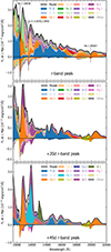 |
Fig. 3. Same as Fig. 2 but for the NIR spectroscopic evolution of the model. |
| In the text | |
|
Fig. 4. Spectroscopic comparisons around peak of our simulated spectra with the observed Ca-rich transients SN 2012hn (Valenti et al. 2014), SN 2019ehk (Jacobson-Galán et al. 2020b; Nakaoka et al. 2021), SN 2010et (Kasliwal et al. 2012), SN PTF11kmb (Lunnan et al. 2017), and SN iPTF16hgs (De et al. 2018). The model epochs are relative to the Sloan r-band peak and have been chosen to match the epochs of each observed spectrum relative to either the Sloan r-band or the Bessel R-band peak. For reference, the strong optical He I features, attributed to the He I 5876, 6678, and 7065 Å lines, are highlighted in cyan and the Ca II NIR triplet is highlighted in pink. |
| In the text | |
|
Fig. 5. Nebular phase spectroscopic comparisons of our simulated spectra at 45 d post r-band peak and the observed Ca-rich transients SN 2021gno (Jacobson-Galán et al. 2022; Ertini et al. 2023), SN 2022oqm (Yadavalli et al. 2024), SN 2019ehk (Jacobson-Galán et al. 2020b; Nakaoka et al. 2021), and SN PTF12bho (Lunnan et al. 2017) at similar epochs. The epochs of the observations are relative to the Sloan r-band or Bessel R-band peak. For reference, the dashed grey line is plotted between the rest wavelengths of the key [Ca II] 7291, 7324 Å lines, the Fe I emission feature predicted by the simulation is highlighted in grey, and the location of the [O I] 6300, 6364 Å feature commonly observed for Ca-rich transients is highlighted in green. |
| In the text | |
Current usage metrics show cumulative count of Article Views (full-text article views including HTML views, PDF and ePub downloads, according to the available data) and Abstracts Views on Vision4Press platform.
Data correspond to usage on the plateform after 2015. The current usage metrics is available 48-96 hours after online publication and is updated daily on week days.
Initial download of the metrics may take a while.