| Issue |
A&A
Volume 702, October 2025
|
|
|---|---|---|
| Article Number | A114 | |
| Number of page(s) | 25 | |
| Section | Extragalactic astronomy | |
| DOI | https://doi.org/10.1051/0004-6361/202554943 | |
| Published online | 14 October 2025 | |
The WISSH quasar project
XII. X-ray view of the most luminous quasi-stellar objects at Cosmic Noon
1
Max-Planck-Institut für Radioastronomie, Auf dem Hügel 69, 53121 Bonn, Germany
2
Dipartimento di Fisica e Astronomia “Augusto Righi”, Università degli Studi di Bologna, Via P. Gobetti 93/2, 40129 Bologna, Italy
3
INAF – Osservatorio di Astrofisica e Scienza dello Spazio, Via P. Gobetti 93/3, 40129 Bologna, Italy
4
INAF – Osservatorio Astronomico di Roma, Via Frascati 33, 00040 Monte Porzio Catone, Italy
5
INAF–OAA, Osservatorio Astrofisico di Arcetri, Largo E. Fermi 5, 50127 Firenze, Italy
6
Space Science Data Center, Agenzia Spaziale Italiana, Via del Politecnico snc, 00133 Roma, Italy
7
Dipartimento di Matematica e Fisica, Università Roma Tre, Via della Vasca Navale 84, 00146 Roma, Italy
8
INAF – Istituto di Astrofisica Spaziale e Fisica Cosmica Milano, Via A. Corti 12, 20133 Milano, Italy
9
Dipartimento di Fisica, Università di Trieste, Via Alfonso Valerio 2, 34127 Trieste, Italy
10
INAF–OAT, Osservatorio Astronomico di Trieste, Via Tiepolo 11, 34131 Trieste, Italy
11
INAF – Istituto di Astrofisica e Planetologia Spaziali, Via Fosso del Cavaliere 100, 00133 Roma, Italy
12
Scuola Normale Superiore, Piazza dei Cavalieri 7, 56126 Pisa, Italy
13
IFPU – Institute for Fundamental Physics of the Universe, Via Beirut 2, 34151 Trieste, Italy
14
Dipartimento di Fisica “G. Occhialini”, Università degli Studi di Milano-Bicocca, Piazza della Scienza 3, 20126 Milano, Italy
15
Department of Physics, Informatics and Mathematics, University of Modena and Reggio Emilia, 41125 Modena, Italy
16
Department of Physics, Middlebury College, Middlebury, VT, 05753
USA
17
Cahill Center for Astronomy and Astrophysics, California Institute of Technology, 1200 California Boulevard, Pasadena, CA, 91125
USA
18
Physics Department, Tor Vergata University of Rome, Via della Ricerca Scientifica 1, 00133 Rome, Italy
19
INFN – Rome Tor Vergata, Via della Ricerca Scientifica 1, 00133 Rome, Italy
20
Centro de Astrobiología (CAB), CSIC-INTA, Camino Bajo del Castillo s/n, 28692 Villanueva de la Cañada, Madrid, Spain
21
Istituto Nazionale di Astrofisica INAF IASF Palermo, Via Ugo La Malfa 153, Palermo, 90146
Italy
⋆ Corresponding author: This email address is being protected from spambots. You need JavaScript enabled to view it.
Received:
1
April
2025
Accepted:
31
July
2025
Abstract
Aims. To improve our knowledge of the nuclear emission of luminous quasi-stellar objects (QSOs) at Cosmic Noon, we studied the X-ray emission of the WISE/SDSS-selected hyper-luminous (WISSH) QSO sample. It consists of 85 broad-line active galactic nuclei (AGN) with bolometric luminosities Lbol > few × 1047 erg s−1 at z ≈ 2 − 4. Our goal is to characterise their X-ray spectral properties and investigate the relation between the X-ray luminosity and the energy output in other bands. To this end, we compared the nuclear properties of powerful QSOs with those derived for the majority of the AGN population.
Methods. We were able to perform X-ray spectral analysis for about one-half of the sample. For 16 sources, we applied the hardness ratio analysis, while for the remaining sources we estimated their 2 − 10 keV intrinsic luminosity L2 − 10; only 8 sources were not detected.
Results. We report a large dispersion in L2 − 10 despite the narrow distribution in Lbol, 2500 Å intrinsic luminosity L2500 Å, and 6 μm intrinsic luminosity λL6 μm of WISSH QSOs (approximately one-third of the sources classified as X-ray-weak QSOs). This suggests that the properties of the X-ray corona and inner accretion flow in hyper-luminous QSOs can be significantly different from those of typical less powerful AGN. The distribution of the X-ray spectral index does not differ from that of AGN at lower redshift and lower Lbol, and does not depend on the Eddington ratio (λEdd) and X-ray weakness. The majority of WISSH QSOs, for which it was possible to estimate the presence of intrinsic absorption (≈65% of the sample), exhibit little to no obscuration (i.e. column density NH ≤ 5 × 1022 cm−2). Among the X-ray obscured sources, we find some blue QSOs without broad absorption lines (BALs) that fall within the ‘forbidden region’ of the Log(NH)−Log(λEdd) plane, which is typically occupied by dust-reddened QSOs and is associated with intense feedback processes. Additionally, we confirm a significant correlation between L2 − 10 and velocity shift of the CIV emission line, a tracer of nuclear ionised outflows.
Conclusions. Multi-wavelength observations of the broad-line WISSH quasars at Cosmic Noon and, in particular, their complete X-ray coverage, allow us to properly investigate the accretion disk–corona interplay to the highest luminosity regime. The distribution of bolometric corrections kbol and X-ray–to–optical indices αOX of the WISSH quasars is strikingly broad, suggesting that caution should be exercised when using Lbol, L2500 Å, and λL6 μm to estimate the X-ray emission of individual luminous QSOs.
Key words: galaxies: active / galaxies: high-redshift / quasars: general / quasars: supermassive black holes / X-rays: galaxies
Member of the International Max Planck Research School (IMPRS) for Astronomy and Astrophysics at the Universities of Bonn and Cologne.
© The Authors 2025
 Open Access article, published by EDP Sciences, under the terms of the Creative Commons Attribution License (https://creativecommons.org/licenses/by/4.0), which permits unrestricted use, distribution, and reproduction in any medium, provided the original work is properly cited.
This article is published in open access under the Subscribe to Open model.
Open Access funding provided by Max Planck Society.
1. Introduction
The X-ray emission from an active galactic nucleus (AGN) carries valuable information on the physical properties of the material distributed over sub-parsec scales around the central supermassive black hole (SMBH; e.g. Turner & Miller 2009), due to inverse Compton scattering of UV accretion disk photons with electrons in the corona. The X-ray spectrum of broad-line Type 1 AGN in the ≈0.3 − 10 keV band can be described by a power law with a slope of Γ ≈ 1.7 − 2. It typically exhibits absorption features due to the presence of ionised outflowing material along the line of sight to the nucleus, with a broad distribution in velocity, distance from the SMBH, ionisation state, and column density (e.g. Krongold et al. 2003; McKernan et al. 2007; Yamada et al. 2024, and references therein). The vast majority of AGN show an extra-continuum emission below 2 keV, called the soft excess, likely related to warm Comptonisation or relativistically blurred reflection from the inner accretion disk (e.g. Miniutti & Fabian 2004; Kubota & Done 2018). Moreover, emission features, such as Fe K emission lines and the broad Compton hump component, which result from fluorescence and reflection off the accretion disk and other sub-parsec material, are also commonly detected above 6 keV (e.g. Matt et al. 1991; Patrick et al. 2012). This picture has basically emerged from an extensive study of local, X-ray-bright, low- to moderate-luminosity AGN with a bolometric luminosity Lbol < 1046 erg s−1 (e.g. Reynolds & Fabian 1995; Ricci et al. 2017).
Our knowledge of the X-ray properties of luminous (Lbol ≥ 1047 erg s−1), highly accreting quasi-stellar objects (QSOs) shining at Cosmic Noon (i.e. z ≈ 2 − 4) is less accurate due to the lack of high-quality X-ray spectra for these distant sources. Nonetheless, during the past two decades XMM-Newton and Chandra observations have provided a large amount of high-z QSOs detected in X-rays. The combination of X-ray data from local AGN and distant QSOs highlights several trends: (i) the intensity of the Fe K line and Compton hump in luminous AGN is weaker than in low-luminosity sources; (ii) the relative contribution of the luminosity in the 2 − 10 keV band (L2 − 10) to Lbol (which approximately corresponds to the UV luminosity in these luminous AGN) progressively decreases as a function of Lbol; (iii) the ratio of the mid-infrared (MIR) luminosity (typically measured at 6 μm) to X-ray luminosity diminishes for increasing Lbol; (iv) a correlation exists between the strength and blueshift of the C IV emission line at 1550 Å, and the X-ray–to–optical index, defined as  (Tananbaum et al. 1979), where L2 keV and L2500 Å are the monochromatic luminosities at 2 keV and 2500 Å, respectively; (v) a sizeable fraction ( ≈ 30%) of luminous QSOs exhibit intrinsic X-ray weakness, i.e. the difference between the measured αOX and that expected from the αOX − Log(L2500 Å) relation is Δ(αOX)≲ − (0.2 − 0.3) (e.g. Vignali et al. 2003; Bianchi et al. 2007; Just et al. 2007; Stern 2015; Zappacosta et al. 2018, 2020; Nardini et al. 2019; Duras et al. 2020; Timlin et al. 2020). These findings highlight the importance of strengthening our understanding of the X-ray properties of luminous high-z QSOs, as well as their complex relationships with other multi-wavelength nuclear parameters. This holds significant potential for uncovering largely unexplored aspects of the accreting SMBH phenomenon, which have remained elusive due to the challenges in obtaining reliable systematic X-ray and multi-band data for such distant AGN populations.
It is widely recognised that luminous QSOs (i.e. highly accreting, billion-solar-mass SMBHs) play a crucial role in the evolution of massive galaxies during Cosmic Noon. In these sources, strong AGN-driven feedback is expected to significantly influence both SMBH growth and star formation activity within the host galaxy (e.g. Silk & Rees 1998; Fiore et al. 2017; Choi et al. 2018; Gaspari et al. 2020; Byrne et al. 2024). Motivated by these results, we have embarked on a comprehensive multi-band investigation on a large sample of broad-line WISE/SDSS-selected hyper-luminous (WISSH) QSOs at z ≈ 2 − 4 (Saccheo et al. 2023). Our goal is to shed light on their nuclear properties, the presence and power of multi-scale multi-phase outflows generated by their huge bolometric radiative output (i.e. Lbol ≈ 1047 − 48 erg s−1), and their host galaxies. The study of these QSOs has revealed the common presence of ionised gas winds, typically with very high velocities relative to the bulk of AGN, at various distances from the central SMBH. Their host galaxies appear to be in a growth phase, with star formation rates of SFR ≈ 102 − 3 M⊙/yr, disturbed kinematics, and that preferentially reside in high-density environments surrounded by companions. The molecular gas content of these host galaxies is typically lower than that of main-sequence galaxies with the same IR luminosity. This combination of a small cold gas reservoir and high SFR suggests that host galaxies of WISSH QSOs may be the progenitors of giant quiescent elliptical galaxies (e.g. Bischetti et al. 2017, 2018, 2021; Duras et al. 2017; Vietri et al. 2018; Bruni et al. 2019; Vietri et al. 2022).
In this paper we extend the initial results on the X-ray properties of a sub-sample of WISSH QSOs reported in Martocchia et al. (2017) and Zappacosta et al. (2020), by presenting the analysis of the X-ray observations that are available for all 85 sources in the sample. The paper is organised as follows. Section 2 describes the X-ray observations used in our investigation and the data reduction. Section 3 presents the X-ray data analysis techniques used depending on the number of collected X-ray photons. The main results are presented in Section 4. In Section 5 we discuss the fraction of intrinsically X-ray-weak sources among QSOs, the relation between some X-ray spectral properties and the Eddington ratio (i.e. the ratio of Lbol to the Eddington luminosity λEdd = Lbol/LEdd), and the comparison with the X-ray properties of QSOs at z > 6. Finally, the summary and our conclusions are given in Section 6. Throughout this work we adopt H0 = 70, Ωm = 0.27, and ΩΛ = 0.73 (Bennett et al. 2013).
2. Observations and data reduction
2.1. Data presentation
All 85 WISSH sources have been observed by Chandra and/or XMM-Newton. Specifically, 53 and 4 objects have single Chandra and XMM-Newton observations, respectively, while 28 have been targeted multiple times (see Figure 1). The complete dataset is presented in Table A.1. In Sections 3 and 4, we consider for each source only the observation with the highest number of X-ray photons.
 |
Fig. 1. X-ray coverage of the WISSH sample. |
We present new proprietary Chandra observations for 44 sources (PI: E. Piconcelli; Prop. ID: 23700190; Cycle 23), which complete the WISSH sample X-ray coverage. We also made use of two proprietary XMM-Newton observations of WISSH59 (PI: C. Pinto), in which the QSO is not the target. Chandra and XMM-Newton archival observations for the remaining 41 sources (Martocchia et al. 2017) were re-analysed to provide a homogeneous analysis of the entire WISSH sample. Finally, for WISSH57, showing peculiar properties in the Chandra spectrum, a Swift-XRT follow-up observation is also presented.
2.2. Chandra observations
We downloaded the data from the Chandra Data Archive1 and reprocessed them through the chandra_repro task using CIAO2 4.14 package with CALDB 4.9.8. Applying the dmcopy tool, we filtered the data and produced an image in the 0.3 − 7 keV energy range. We inspected the image with SAOIMAGEDS93 to define the extraction regions, selecting circular regions of radii ≈2 arcsec and ≈11 − 42 arcsec for the source and background, respectively. The source extraction region was defined to correspond to ≈90% of the encircled energy fraction, while the background one was selected to be free of sources and close enough to the target to be representative of the background in the source extraction region. Once the source and background regions were identified, spectral extraction was performed with CIAO task specextract, which also produces the Auxiliary Response File (ARF) and the Redistribution Matrix File (RMF).
2.3. XMM-Newton observations
EPIC pn Observation Data Files (ODFs) were downloaded from XMM-Newton Science Archive4 (XSA). We reprocessed them using version 20.0.0 of the XMM-Newton SAS (Gabriel et al. 2004) and produced the event files through the epproc task. Extracting the light curve in the 10 − 12 keV energy range, we checked for possible presence of flaring background, typically attributed to soft protons. Accordingly, the event files were filtered with either espfilt or gtigen tool, producing Good Time Interval (GTI) tables, and light curves were re-extracted. Finally, we created cleaned event files in the energy range 0.3 − 10 keV. A circular region of radius ≈10 − 15 arcsec (corresponding to ≈70% of the encircled energy fraction) was used for the source. This choice limits the background contribution and is well suited for relatively faint X-ray sources. A circular region of radius ≈15 − 55 arcsec was used for the background, instead. Spectra were extracted through the XMM-Newton SAS meta-task especget, which runs also the arfgen, rmfgen and backscale tasks. Thus, ARF and RMF matrices are calculated, and the source and background extraction region are re-scaled to obtain the spectra.
2.4. Swift-XRT observation
The Swift-XRT observations of WISSH57 have been performed in photon counting (PC) readout mode. Data were first reprocessed thanks to the on-the-fly facilities developed by the ASI-SSDC and included in the NASA-HEASARC HEASOFT package5 (version v6.31.1). The data processing relied on the XRTDAS software package and the standard calibration, filtering processing steps were taken, and the calibration files available CALDB (version 20220803) used. For each of the three exposure available for WISSH57, the source spectrum was extracted using a circle of 20-pixel (≈47 arcsec) radius centred on the target. The background was computed adopting a circular region with a radius of 40 pixels centred on a blank area. The resulting spectra were stacked.
3. Data analysis
Depending on the number of detected X-ray photons, the sources were divided into three groups as follows:
-
39 QSOs with ≥20 net (i.e. background-subtracted) counts;
-
16 QSOs with 5 < net counts < 20;
-
30 QSOs with ≤5 net counts (8 of them are undetected).
Their X-ray properties are presented in the following sections. For all parameters, errors and upper limits are reported at 1σ and 90% confidence level, respectively.
3.1. Analysis of the HC-WISSH sub-sample
In this paper we refer to > 5 counts sources as the High-Counts WISSH (HC-WISSH) sub-sample.
3.1.1. Analysis of QSOs with ≥20 counts: spectral fitting
For the QSOs corresponding to ≥20 counts (maximum value: ≈2500 counts; median value: ≈140 counts), we performed basic/moderate-quality spectral analysis. Thus, we derived the continuum X-ray properties (Γ and the intrinsic column density NH), along with the observed 0.5 − 10 keV flux (F0.5 − 10) and the intrinsic 2 − 10 keV luminosity, through the X-ray spectral fitting package XSPEC (Arnaud 1996). Errors on F0.5 − 10 and L2 − 10 were calculated using the cflux and clumin tools in XSPEC. These are convolution models to calculate the flux of all the components included in the best fit spectral model.
We grouped spectral points to one count/bin with the grppha tool of the FTOOLS package6. Cash statistics with direct background subtraction (C-stat in XSPEC; Cash 1979; Wachter et al. 1979) was used for the spectral fitting. We initially adopted a power law model modified by Galactic absorption (see Table B.1), which translates into an XSPEC model of the form phabs*po. We also tested the presence of intrinsic absorption by adding a zphabs multiplicative component. For about one-third of the analysed QSOs, this addition yielded to an improvement in the fit quality with respect to the power law model by > 95% confidence level using an F-test. We therefore included an absorption component in the best fit model used to calculate fluxes and luminosities reported in Table B.1. If an additional intrinsic obscuring component was not significantly required, an upper limit is reported in the NH column of Table B.1. As an example, in Figure 2a we report the Chandra spectrum of WISSH47. We detect ≈130 counts for this source in the 0.3 − 7 keV energy range, which is representative of the median number of counts for the ≥20 net counts sub-sample, and find a significant NH (i.e. > 95% confidence). Figure 2b shows the NH − Γ confidence contours using the best fit model.
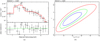 |
Fig. 2. (a) Chandra spectrum (re-binned for display purposes) of WISSH47 (z = 2.6987). We detect about 130 counts for this source and measure significant intrinsic absorption. The residuals are defined as (data – model) in units of σ. (b) NH − Γ contour plot for the best fit model of WISSH47. The blue, green, and red curves represent the 68%, 90%, and 99% confidence levels, respectively. |
3.1.2. Analysis of QSOs with 5 < counts < 20: hardness ratio analysis
For the QSOs detected with 5 − 20 photons, we derived the number of soft (0.5 − 2 keV, S) and hard (2 − 10 keV, H) source and background photons. These values, normalised by the different source and background extraction areas, were required to derive the hardness ratio (HR)
 (1)
(1)
through the Bayesian Estimator of Hardness Ratio (BEHR) (Park et al. 2006). BEHR is especially useful in Poissonian regimes, where the background subtraction is not a good solution, as correctly deals with the non-Gaussian nature of the error propagation, whether or not the source is detected in both bands. Then, we constrained intrinsic NH comparing the measured HR with the values from simulated absorbed power law models with fixed Γ = 1.8 (Piconcelli et al. 2005), which also take into account the sources redshift. NH was considered to be significant when its 1σ lower boundary was not consistent with zero, otherwise upper limits on NH were derived. One-fourth of the objects in the sub-sample exhibit a significant NH.
We calculated F0.5 − 10 through Chandra WEBPIMMS7, assuming Γ = 1.8 and the Galactic absorption. L2 − 10 was derived as
 (2)
(2)
where dL is the luminosity distance8,  (derived using WEBPIMMS) is the 2 − 10 keV flux corrected for Galactic and intrinsic absorption, z is the source redshift and Γ = 1.8. Results are reported in Table B.2.
3.2. Analysis of QSOs with ≤5 counts and non-detections
We adopted the binomial method of Weisskopf et al. (2007) (see their Appendix A.3) and derived the probability distribution function of net counts, to test whether the sources having ≤5 counts could be considered detected or not. The nominal value of the net counts coincides with the peak of the probability distribution. As in Section 3.1.2, we derived F0.5 − 10 through WEBPIMMS, assuming Γ = 1.8 and the Galactic absorption. L2 − 10 were obtained from Equation (2), assuming NH = 5 × 1022 cm−2, which is the median value for the 14 absorbed sources in the HC-WISSH sample9; their values with and without NH change, on average, by ≈7%. Results are reported in Table B.3. Only 8 sources result to be undetected (detection significance is at 99% confidence level).
3.3. QSOs with multiple observations
For the 28 out of 85 QSOs that have multiple observations (see Figure 1), we evaluated possible changes in terms of NH, observed 0.5 − 2 keV flux (F0.5 − 2) and observed 2 − 10 keV flux (F2 − 10). We did not consider Γ variability, as we do not have a spectroscopic estimate of this parameter for all of the observations; moreover, even when available, it has non-negligible uncertainties. We report the most significant cases of variability, set to > 2σ confidence level for what concerns NH variability (to spot candidate changing look AGN) and to > 3σ confidence level for flux variability. Results are presented in detail in Appendix C. In particular:
-
two QSOs (WISSH59 and WISSH69) show intrinsic NH variability of up to an order of magnitude (as fast as ≈40 days rest-frame in case of WISSH59);
-
four QSOs (WISSH13, WISSH33, WISSH35 and WISSH63) show F0.5 − 2 variability (as fast as ≈9 days rest-frame in case of WISSH35);
-
three QSOs (WISSH70, WISSH82 and WISSH83) show both F0.5 − 2 and F2 − 10 variability (as fast as ≈120 days rest-frame in case of WISSH83).
We also checked for possible coincidence of WISSH objects with the eROSITA eRASS1 Main catalogue sources (Merloni et al. 2024). We find seven cross-identifications (i.e. WISSH14, WISSH27, WISSH29, WISSH37, WISSH49, WISSH54, WISSH60) within a 5 arcsec radius. Comparing the 0.2 − 2.3 keV fluxes (eROSITA sensitivity is maximum in this band), we find a > 3σ variability over ≈6 years rest frame for WISSH60, which has a high detection significance both in Chandra and eROSITA observation. Even assuming Γ = 1.7 as for eROSITA, only WISSH60 exhibits a flux variation > 3σ.
Finally, as the WISSH57 Chandra observation exhibits a particularly steep Γ = 2.80 ± 0.32, we submitted a request for a follow-up observation with Swift-XRT. The observation yields a more standard  . Although possibly tracing a rapid (≈4 months rest-frame) spectral change, the photon index variability is < 3σ due to the large uncertainties affecting both measurements.
4. Results
4.1. Intrinsic absorption, X-ray luminosity and X-ray bolometric correction
Figure 3 shows the NH distribution derived for the HC-WISSH sub-sample. The bulk ( ≈ 76%) of the sources exhibits low level of intrinsic absorption (NH < 1022 cm−2). We note, however, that ≈15% of the QSOs are strongly obscured (NH ≥ 1023 cm−2). Sources for which the power law model with no absorption represents the best fit are included in the bin NH < 5 × 1021 cm−2 (orange bar). For each QSO, the intrinsic L2 − 10 was derived by correcting for nuclear obscuration NH. In Figure 4, L2 − 10 is shown as a function of Lbol, taken from Saccheo et al. (2023) who performed multi-band SED fitting after correcting for dust extinction for all WISSH sources. The scaled axis highlights the large L2 − 10 distribution compared to the narrow Lbol distribution.
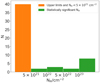 |
Fig. 3. Intrinsic column density distribution for the HC-WISSH sample. Sources for which the power law model represents the best fit (i.e. unobscured) are included in the bin NH < 5 × 1021 cm−2. |
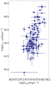 |
Fig. 4. Log(L2 − 10) as a function of Lbol for the entire WISSH sample. |
We also calculated the hard X-ray bolometric correction kbol = L2 − 10/Lbol. In Figure 5, the kbol of WISSH QSOs is reported as a function of Lbol, along with other low- and high-Lbol AGN samples from literature. We distinguished between broad absorption line (BAL) and non-BAL WISSH objects (as listed in Bruni et al. 2019, and shown as indigo and purple stars, respectively), since a sizeable fraction of BAL sources has been found to be intrinsically X-ray weak (e.g. Luo et al. 2014; Vito et al. 2018). The XMM-COSMOS sample of 343 Type 1 AGN presented by Lusso et al. (2010, L10 hereafter), which constitutes the bulk of low-luminosity AGN, is shown with yellow dots. The 22 SUBWAYS QSOs and Type 1 AGN with Lbol > 1045 erg s−1 from Matzeu et al. (2023) can be seen as red dots. Light blue triangles correspond to the 14 radio-quiet high-λEdd (λEdd ≳ 1) sources at z ≈ 0.5 published by Laurenti et al. (2022). The sample of luminous and intrinsically blue QSOs at z ≈ 3 presented by Trefoloni et al. (2023), for which constrained L2 − 10, Γ, λEdd, and CIV line velocity values are available, is shown as pink squares. The black solid line represents the relation that Duras et al. (2020) (D20, hereafter) found fitting Type 1 sources only, while the black dashed curves correspond to the 0.26 dex spread of the same relation.
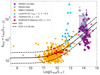 |
Fig. 5. Bolometric correction as a function of Log(Lbol). WISSH BAL and non-BAL QSOs are shown as indigo and purple stars, respectively. The XMM-COSMOS sample of 343 Type 1 AGN presented by L10 is represented by yellow dots; it covers a wide range of redshifts (0.04 < z < 4.25) and X-ray luminosities (40.6 ≤ Log(L2 − 10/erg s−1)≤45.3). The 22 SUBWAYS QSOs and Type 1 AGN at intermediate redshifts (0.1 ≲ z ≲ 0.4) from Matzeu et al. (2023) can be seen as red dots. Light blue triangles correspond to the 14 radio-quiet high-λEdd (λEdd ≳ 1) QSOs at 0.4 ≤ z ≤ 0.75 presented by Laurenti et al. (2022). The sample of luminous and intrinsically blue QSOs at z ≈ 3 presented by Trefoloni et al. (2023), for which constrained L2 − 10, Γ, λEdd, and CIV line velocity values are available, are shown as pink squares. The black solid and dashed lines correspond to D20 best fit to Type 1 sources and its 0.26 dex spread, respectively. |
The huge spread of WISSH QSOs in the kbol − Log(Lbol) plane was already apparent (although with half of the current sources) in Martocchia et al. (2017). This spread looks more evident due to the relatively narrow range of Lbol sampled by WISSH objects. Figure 6a shows the ratio of the observed kbol to the expected values at the same Lbol measured using the D20 relation (kbol/kbol, D20; symbols are the same as in Figure 5). WISSH BAL QSOs are mainly (≈56%) located above the D20 relation including its spread: at a given Lbol, they are more often characterised by relatively weak X-ray emission. Nonetheless, non-negligible fractions of ≈41% and ≈3% of WISSH BAL QSOs fall within and below D20 spread, respectively. Conversely, non-BAL objects are more equally distributed: ≈31% above, ≈30% within and ≈39% below the best fit relation. To summarise, only ≈34% of the whole WISSH sample falls within the prediction of the D20 relation (including its spread), while ≈66% is distributed above ( ≈ 41%) or below ( ≈ 25%) it. The complete distribution for WISSH QSOs is visible in Figure 6b, where BAL and non-BAL sources are reported as indigo and purple bars, respectively.
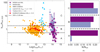 |
Fig. 6. (a) Ratio of measured kbol values to expected kbol values from D20 as a function of Log(Lbol). WISSH QSOs are compared to literature samples; the symbols are the same as in Figure 5. The two black dashed lines correspond to the 0.26 dex spread of D20 best fit to Type 1 sources. (b) Distribution of WISSH QSOs kbol with respect to the D20 relation, including its spread (black horizontal dashed lines), i.e. being below, within, or above it. BAL and non-BAL sources are represented as indigo and purple bars, respectively. |
4.2. Distribution of αOX and the fraction of X-ray-weak WISSH QSOs
We derived αOX for WISSH QSOs using L2500 Å from Saccheo et al. (2023). Figure 7 displays the αOX − Log(L2500 Å) plane, where WISSH QSOs are compared to literature samples. Symbols are the same as in Figure 5. The relations by Martocchia et al. (2017), L10 and Just et al. (2007) (black dashed, solid and dotted line, respectively) are also reported as representative of the numerous literature works. The WISSH sample occupies the bottom-right region of the plane, meaning that luminous QSOs are among the X-ray-weakest sources. This result is expected, given the indications of Figure 5, where high kbol, corresponding to low αOX values, implies a low coronal X-ray contribution to the overall AGN emission, i.e. most of the accretion-related luminosity comes from the accretion disk in the UV band (but see also models of Kubota & Done 2018). As in the kbol − Log(Lbol) plane, WISSH QSOs broadly follow the decreasing αOX trend at increasing L2500 Å, as proposed by previous papers and already observed by Martocchia et al. (2017), though with lower statistics.
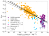 |
Fig. 7. X-ray–to–optical index (αOX) as a function of Log(L2500#x2004;Å). WISSH QSOs are compared to literature samples; the symbols are the same as in Figure 5. The black dashed, solid, and dotted lines are the best fits from Martocchia et al. (2017), L10, and Just et al. (2007), respectively. In particular, L10 fit XMM-COSMOS data only; Just et al. (2007) consider 34 QSOs of their core sample, 332 sources from Steffen et al. (2006), and 14 from Shemmer et al. (2006); and Martocchia et al. (2017) consider XMM-COSMOS objects, 23 optically selected QSOs from the Palomar-Green (PG) Bright QSO Survey of the complete sample by Laor et al. (1994) and the 41 WISSH QSOs with available X-ray data at the time of the publication. |
Measuring the offset between the observed values (αOX) and those expected from L10 relation (αOX, L10) at a given L2500 Å, one can define Δ(αOX) as
 (3)
(3)
This quantity can be used to point out X-ray-weak sources, characterised by Δ(αOX)≤ − 0.2 (Luo et al. 2015). Figure 8 shows the Δ(αOX) distribution of WISSH QSOs (see also Table E.1). About 31% of them falls under the X-ray-weak category, which is highlighted by the grey-shaded area in Figure 8. It is evident that BAL and non-BAL QSOs are differently distributed. The Kolmogorov-Smirnov test results in p = 0.003, which rejects the two-sided null-hypothesis probability that the two distributions are derived from the same parent distribution at 3σ confidence level. In particular, Δ(αOX) value is below the adopted threshold for ≈47% and ≈20% of BAL and non-BAL objects, respectively. X-ray-weak sources are therefore much more common among BAL objects than non-BAL ones. In case of QSOs with multiple X-ray observations (see Section 3.3), we report no X-ray weak to X-ray normal (or vice versa) transitions.
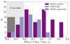 |
Fig. 8. Δ(αOX) = αOX − αOX, L10 distribution. αOX, L10 refers to the value derived from the L10 relation at a given L2500 Å. The BAL and non-BAL QSOs are represented as indigo and purple bars, respectively. The grey bar is for undetected sources, which have all been included in the X-ray-weakest bin. The grey-shaded area highlights the locus of X-ray-weak sources. |
4.3. Photon index distribution
To provide a deeper investigation of the possible origin of X-ray weakness in the presence of an absorbing column density, we searched for a possible correlation between Γ and Δ(αOX). Indeed, additional absorption, if not included in the X-ray spectral analysis, would result in X-ray-weak AGN to have a flatter photon index.
We only considered the sources with ≥20 photons, for which we derived Γ through X-ray spectral analysis. In Figure 9a, Γ is derived applying a power law model modified by Galactic absorption, while in Figure 9b we also take into consideration the presence of intrinsic absorption (see Section 3.1.1). The main variations occur at the lowest Δ(αOX): the suppression of the soft X-ray emission by intrinsic NH causes both Γ flattening and X-ray weakening with respect to the optical/UV emission. However, once the best spectral model is applied (Figure 9b), the Pearson correlation test only results in p = 0.01, i.e. Δ(αOX) and Γ correlate at less than 3σ significance level. Although we cannot rule out the possibility of additional obscuration among the X-ray-weakest sources, it is clear that the roughly uniform spectral shape as a function of Δ(αOX) makes it unlikely that extra-absorption is responsible for the X-ray-weak phenomenon in our sample.
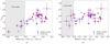 |
Fig. 9. X-ray photon index as a function of Δ(αOX) for the sources with ≥20 counts. (a) Γobs derived using a power law model modified by Galactic absorption. (b) Cold absorption component included in the spectral model used to derive Γ (see Section 3.1.1). The BAL and non-BAL QSOs are represented as indigo and purple dots, respectively. The grey-shaded areas highlight the locus of X-ray-weak sources. |
For 36 sources (≈42% of WISSH QSOs), a black hole mass (MBH) estimate is available (Bischetti et al. 2017; Vietri et al. 2018, and in prep.). MBH were derived through a single epoch virial method relation (Bongiorno et al. 2014), which depends on the Hβ line Full Width at Half Maximum (FWHMHβ) and the continuum luminosity at 5100 Å (λLλ):
 (4)
(4)
The systematic uncertainty in the Log(MBH) determination is estimated to be about 0.3 dex (Bongiorno et al. 2014). From the MBH values, we calculated the Eddington luminosity, which spans the range LEdd ≈ 3 × 1047 − 3 × 1048 erg s−1. Having both LEdd and Lbol, we derived the Eddington ratios λEdd. This results in a range between 0.2 and 2.9, with a median value 0.6. These numbers indicate a high-accretion regime, as expected for the most luminous QSOs at Cosmic Noon (e.g. Hopkins et al. 2007; Merloni & Heinz 2008; Delvecchio et al. 2014).
For the 19 WISSH sources which have both an available MBH and ≥20 photons to perform X-ray spectral analysis, we also studied Γ as a function of λEdd. This relation may be expected as higher λEdd corresponds to more intense disk emission, thus a more efficient coronal Compton cooling, which leads to a softer (i.e. steeper) photon index (e.g. Haardt & Maraschi 1991, 1993; Pounds et al. 1995; Fabian et al. 2015; Cheng et al. 2020). The results are shown in Figure 10, where symbols for literature samples are the same as in Figure 5. WISSH sources are represented as blue stars, while the black solid, dashed, dotted and dash-dotted lines correspond to Liu et al. (2021) and Brightman et al. (2013) relations, and two models (BCES bisector and FITEXY method) from Trakhtenbrot et al. (2017), respectively. In order to quantify the distribution in the Γ − Log(λEdd) plane, we fitted a linear model to the data in a Bayesian framework using the python package linmix (Kelly 2007). The Pearson correlation test results in p = 0.07, suggesting no significant correlation. This highlights the importance of populating the plane with high-λEdd QSOs.
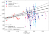 |
Fig. 10. X-ray photon index as a function of Log(λEdd). Only WISSH QSOs with ≥20 photons (i.e. with X-ray spectral analysis), for which an estimate of MBH is available are considered. The symbols are the same as in Figure 5, with the exception of WISSH sources, which are represented as blue stars. The black solid, dashed, dotted, and dash-dotted lines correspond to the Liu et al. (2021) and Brightman et al. (2013) relations, and two models (BCES bisector and FITEXY method) from Trakhtenbrot et al. (2017), respectively. Specifically, Liu et al. (2021) consider 47 AGN with both super- and sub-Eddington accretion rates from the sample compiled by the SEAMBH collaboration (Du et al. 2018). Brightman et al. (2013) use 69 broad-line AGN from the extended Chandra Deep Field South and COSMOS surveys. Trakhtenbrot et al. (2017) refer to 228 hard X-ray selected AGN at 0.01 < z < 0.5, drawn from the Swift/BAT AGN Spectroscopic Survey (BASS, Baumgartner et al. 2013). |
4.4. The Log(NH)−Log(λEdd) diagram
In the context of studying AGN evolution from an early, dust-reddened, obscured phase to a later, blue and unobscured one, Fabian et al. (2008) introduced the Log(NH)−Log(λEdd) plane. Specifically, they identified a region of this plane which can be associated with a transitional blow-out phase in AGN evolution, during which the nuclear source, previously obscured, is set free from absorbing gas thanks to AGN-driven feedback via nuclear winds. In this scenario, the high-NH/high-λEdd conditions correspond to a ‘forbidden region’ in the plane (grey-shaded in Figure 11). Following Fabian et al. (2008) and Ishibashi et al. (2018), they assumed a dusty gas of partially ionised hydrogen, and took into consideration the trapping of reprocessed radiation by dusty gas. In Figure 11, maximal- and no-photon trapping regimes are represented as a black solid and dashed line, respectively.
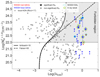 |
Fig. 11. Intrinsic column density (derived assuming Γ = 1.8) as a function of Log(λEdd). QSOs from the HC-WISSH sample with available MBH are plotted. WISSH BAL objects are contoured with a turquoise line. X-ray-weak QSOs (Δ(αOX) < − 0.2) are surrounded with a green circle. Blue and red QSOs are shown in the corresponding colour. Stars correspond to sources for which intrinsic absorption is significantly detected (see Sections 3.1.1 and 3.1.2). QSOs from Ricci et al. (2017) are shown as grey crosses. Black solid and dashed lines are Ishibashi et al. (2018) and Fabian et al. (2008) relations, derived from a maximal- and no-photon trapping model, respectively. The black horizontal dotted line indicates NH = 1022 cm−2. |
We populated the Log(NH)−Log(λEdd) plane combining the available information on MBH and NH of the sources from the HC-WISSH sample. To better constrain NH, we fixed the X-ray continuum slope to Γ = 1.8 (e.g. Piconcelli et al. 2005), since it does not vary significantly within its uncertainties, as shown in Figure 9b. Specifically, WISSH sources exhibit an average photon index Γ = 1.88 ± 0.29 (where the reported error is the dispersion of the distribution). The vast majority of WISSH objects are optically classified as blue sources, while only seven QSOs (i.e. WISSH25, WISSH34, WISSH40, WISSH49, WISSH58, WISSH66, WISSH74) exhibit a colour excess E(B − V)≥0.15, accordingly to Saccheo et al. (2023), and can be classified as dust-reddened broad-line sources. Figure 11 reports WISSH BAL objects contoured with a turquoise line. X-ray-weak QSOs (Δ(αOX) < − 0.2) are surrounded with a green circle. Blue and red QSOs are shown in the corresponding colour. Stars correspond to sources for which intrinsic absorption is significantly detected (see Sections 3.1.1 and 3.1.2). Sources from the large sample of local AGN presented by Ricci et al. (2017) are also reported (grey crosses) and typically populate the Log(NH)−Log(λEdd) plane outside the forbidden region. All but one of WISSH sources with significantly detected NH located in the forbidden region are blue QSOs. Surprisingly, among them, non-BAL QSOs are X-ray-weak sources, while BAL QSOs show Δ(αOX) > − 0.2. Finally, unlike what is commonly found for red QSOs (e.g. Lansbury et al. 2020), WISSH40 falls outside the forbidden region.
4.5. X-ray versus mid-infrared luminosity
The X-ray and MIR emissions are strictly connected in QSOs. The former is coronal emission of accretion disk Comptonised photons, and the latter is due to reprocessed accretion disk emission being thermalised by the dusty torus. Thus, a positive correlation is expected in the X-ray – MIR luminosity plane (e.g. Gandhi et al. 2009). By construction, all 85 WISSH QSOs have been detected in the WISE 3.3 μm band, from which the luminosity at 6 μm (λL6 μm in Table E.1) can be recovered applying a correction derived from the mean SED of the sample (Saccheo et al. 2023). This allowed us to study the X-ray–MIR relation in the highest luminosity regime, while most of previous works focused on the low-luminosity regime (e.g. Lutz et al. 2004; Fiore et al. 2009; Lanzuisi et al. 2009; Mateos et al. 2015; but see also Stern 2015, S15 hereafter, and Chen et al. 2017).
Figure 12a shows the intrinsic L2 − 10 as a function of λL6 μm. WISSH BAL and non-BAL objects are indigo and purple stars, respectively, while grey dots are AGN from the samples of Lanzuisi et al. (2009), Mateos et al. (2015) and S15. The black solid, dashed and dotted lines are S15, Lanzuisi et al. (2009) and Chen et al. (2017) relations, respectively. Despite the limited range in terms of Log(λL6 μm) due to the sample selection, WISSH sources cover a wide range of Log(L2 − 10). Nonetheless, they seem to agree with the luminosity-dependent trends found by S15 and Chen et al. (2017), who report a flattening at the highest MIR luminosities. Since the MIR luminosity in AGN is strongly linked to the reprocessing of UV accretion disk emission, this behaviour has been interpreted within the framework of the αOX − LUV relation (e.g. Chen et al. 2017).
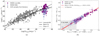 |
Fig. 12. (a) Intrinsic 2 − 10 keV luminosity as a function of λL6 μm. WISSH BAL and non-BAL objects are shown as indigo and purple stars, respectively, while the grey dots represent various comparison samples from Lanzuisi et al. (2009), Mateos et al. (2015), and S15. The black solid, dashed, and dotted lines correspond to the relation by S15, Lanzuisi et al. (2009), and Chen et al. (2017), respectively; (b) Δ(αOX) as a function of the L2 − 10 offset of WISSH QSOs from the relation by S15 (Δ6 μm, X). WISSH BAL and non-BAL objects are indigo and purple dots, respectively. The grey-shaded area highlights the X-ray-weak region of the plane. The dispersion around the best fit (solid red line) is given by plotting ≈200 realisations considering the values of slope and intercept within 1σ of the sampled marginalised posterior distribution. |
Similarly to the derivation of Δ(αOX), we studied the offset of WISSH QSOs measured Log(L2 − 10) from the one expected from S15 relation Log(L2 − 10, S15):
 (5)
(5)
In Figure 12b, Δ6 μm, X is compared to Δ(αOX). WISSH BAL and non-BAL objects are indigo and purple dots, respectively. We fitted the positive correlation with a first order model using the hierarchical Bayesian model linmix (see Section 4.3), resulting in the following tight relation:
 (6)
(6)
This robust relation (p = 3 × 10−50; Pearson correlation coefficient rP = 0.97; see Figure D.1a and Table D.1) makes it possible to translate the Δ(αOX)-based definition of X-ray-weak sources into the Δ6 μm, X parameter, resulting in Δ6 μm, X ≤ −0.52. The X-ray-weak region of the Δ(αOX)−Δ6 μm, X plane is highlighted by the grey-shaded area. We notice that once L2500 Å and λL6 μm are known, both Equations (3) and (5) can be expressed as a function of L2 − 10 (assuming a photon index, e.g. Γ ≈ 1.8 − 2, to estimate L2 − 10 from L2 keV). Therefore, L2 − 10 can be derived through Equation (6). This would provide less ambiguous results, thanks to the narrow distribution of the sources in the Δ(αOX)−Δ6 μm, X plane compared to the spread exhibited by WISSH QSOs in the Log(L2 − 10)−Log(λL6 μm) plane. In addition, the comparison between L2 − 10 and the observed 2 − 10 keV luminosity can provide an estimate of the intrinsic NH.
4.6. The Log(L2 − 10)−vCIV and Δ(αOX)−vCIV relations
A weak but significant correlation has been reported between αOX and Δ(αOX), and CIV emission line blueshift (tracing the velocity of BLR-scale ionised winds) (e.g. Kruczek et al. 2011; Richards et al. 2011; Ni et al. 2018; Vietri et al. 2018; Timlin et al. 2020), suggesting a link between the shape of the AGN SED and the capability of accelerating winds from the nuclear region. This is not surprising, as it is worth noting that a substantial ionising flux, such as QSO X-ray emission, can overionise the gas surrounding the accreting SMBH, thereby preventing the launch of strong nuclear winds (e.g. Proga 2007, and references therein). Nonetheless, given their large radiative output and high accretion rate, the most luminous AGN (Lbol ≥ 1047 erg s−1) are expected to give rise to the most powerful winds (e.g. Faucher-Giguère & Quataert 2012; Giustini & Proga 2019; Ward et al. 2024) as supported by a wealth of observations over the last decade (e.g. Fiore et al. 2017; Vietri et al. 2018; Meyer et al. 2019; Perrotta et al. 2019; Musiimenta et al. 2023).
Interestingly, Zappacosta et al. (2020) reported the discovery of a relation between L2 − 10 and CIV blueshift, based on a small sub-sample of WISSH QSOs. Due to the narrow UV luminosity range covered by the WISSH sources, this supports a scenario in which faster nuclear outflows are unequivocally associated with high-luminosity QSOs that exhibit weaker X-ray emission. We further investigated this relation by taking advantage of the wide X-ray coverage of WISSH QSOs presented in Section 3 and the increase in the number of WISSH QSOs with measured CIV velocity vCIV10 (Vietri et al., in prep.). We did not consider BAL objects because of absorption features preventing a proper estimate of the CIV emission line properties. As shown in Figure 13 (top panel), we confirm the presence of a strong (rP = 0.77) and highly significant (p = 5 × 10⁻⁶) correlation between Log(L2 − 10) and vCIV. In order to quantify the distribution in the Log(L2 − 10)−vCIV plane, we fitted a linear model to the data using the hierarchical Bayesian model linmix (see Section 4.3), resulting in Log(L2 − 10) = (1.84 ± 0.34)×10−4vCIV + (46.08 ± 0.14).
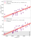 |
Fig. 13. Intrinsic 2 − 10 keV luminosity (top panel) and Δ(αOX) (bottom panel) as a function of CIV velocity vCIV. WISSH non-BAL objects are shown as purple dots. The dispersion around the best fits (solid red lines) is given by plotting ≈200 realisations considering the values of slope and intercept within 1σ of the sampled marginalised posterior distribution (see Figures D.1b and D.1c, and Table D.1 for further details). |
We also confirm the presence of a robust correlation (p = 4 × 10⁻⁶; rP = 0.82) between Δ(αOX) and vCIV for WISSH QSOs (Figure 13, bottom panel). Using linmix, we obtain Δ(αOX) = (7.01 ± 1.19)×10−5vCIV + (0.22 ± 0.05).
5. Discussion
5.1. Fraction of X-ray-weak sources among luminous QSOs
WISSH QSOs are ideal sources for probing the extreme ends of Lbol, L2500 Å and λL6 μm distributions, and they encompass the most extreme values of kbol, αOX and λEdd within the AGN population, as shown in Figures 5, 7, 10 and 12a. WISSH sources follow the kbol − Log(Lbol) and αOX − Log(L2500 Å) trends derived from samples of AGN at lower luminosities, confirming that L2 − 10 becomes relatively weak with increasing AGN luminosity. This suggests that the accretion disk – X-ray corona coupling is not subject to a sudden change for the bulk of the most luminous AGN population, but instead evolves consistently with what predicted by the well-known kbol − Log(Lbol) and αOX − Log(L2500 Å) relations. Nevertheless, it is clear from Figures 5, 7 and 12a that WISSH QSOs exhibit distinctive distributions. Due to their selection, these sources cover a narrow range of Lbol, L2500 Å and λL6 μm values. Despite this, they show a highly dispersed distribution of kbol, αOX and Δ6 μm, X values. It is worth noting that the complete X-ray coverage of WISSH has been crucial in revealing this feature, which was only suggested by Martocchia et al. (2017) based on a smaller sample of sources with X-ray data.
We adopted the threshold Δ(αOX)≤ − 0.2 from Luo et al. (2015) to identify X-ray-weak QSOs. About 31% of WISSH sources fall below the threshold: specifically, ≈43% of BAL and ≈20% of non-BAL QSOs (Figure 8). Therefore, although the fraction of intrinsically X-ray-weak sources is much higher in BAL QSOs, this phenomenon is also present in a sizeable fraction of normal QSOs, suggesting it must be considered relevant for the entire population of highly accreting and luminous AGN, in agreement to the results presented by Nardini et al. (2019) and Laurenti et al. (2022).
A large λEdd value seems to have a key role in triggering a weak state of the X-ray corona. The launch of powerful nuclear winds due to the increasing importance of radiation pressure can affect (and, possibly, remove) the innermost part of the accretion disk (i.e. the source of optical/UV seed photons) which is believed to be surrounded by the X-ray corona. X-ray weakness compared to UV emission is therefore fundamental to avoid nuclear gas over-ionisation, which would prevent radiation pressure from producing radiatively driven winds (e.g. Proga 2003, 2007; Leighly 2004; Xu et al. 2024). Figure 13 supports this scenario for WISSH objects, showing that the QSOs with the most negative Δ(αOX) values typically host the fastest nuclear ionised winds.
The physical and geometrical properties of the inner accretion disk can be different in high-λEdd environments, as the enhanced radiation pressure driven by photon trapping favours the presence of slim (i.e. geometrically thick) accretion flow characterised by a low radiation efficiency (e.g. Abramowicz et al. 1988; Cao & Gu 2022). Furthermore, size and location of the X-ray corona itself could depend on the accretion rate and trigger intrinsic X-ray weakness due to a significant reduction of the active region and/or strong light bending, as suggested by Miniutti et al. (2012). Recent simulations of high-λEdd AGN presented by Pacucci & Narayan (2024) show that the X-ray SED may depend on the SMBH spin and on the inclination of our line of sight, due to the presence of a puffed-up structure of the hot inner accretion flow in these sources. Slowly spinning SMBHs are associated with the X-ray-weakest sources with extremely steep (i.e. Γ > 3) SEDs. In case of spinning SMBHs, the effect of the viewing angle is important for observing stronger X-ray emission and a continuum with flatter slopes as the inclination decreases. Inayoshi et al. (2024) recently argued that X-ray weakness of AGN with high-λEdd accretion disks can be related to the presence of a warm X-ray corona with large optical depth which produces a significant softening of the X-ray continuum, leading to hard X-ray flux reduction. This steepening of the X-ray spectral slope is not observed in WISSH QSOs (see Figure 9). However, most of the X-ray-weak sources in the WISSH sample do not have a measured Γ and, therefore, it is not possible to completely rule out this scenario. Similarly, we cannot exclude that part of the X-ray continuum emission is scattered off our line of sight by a highly ionised medium with large NH and small covering factor, as suggested by Laurenti et al. (2022).
Finally, multiple X-ray observations of some WISSH QSOs offered the opportunity to detect possible transitions from an intrinsic X-ray-weak state to a normal state (and vice versa) over very different timescales (i.e. from a few days to years). However, none of those sources underwent such change, as reported in Appendix C. Future well-designed campaigns to monitor the X-ray emission of WISSH QSOs will be useful to shed light on the occurrence of these transitions, their timescales, the fraction of persistent, intrinsically X-ray-weak sources among the most luminous QSOs, and the duration of the X-ray-weak phase. These insights are essential for providing constraints, which are currently unavailable, to improve our understanding of the accretion disk – corona system in AGN with high accretion rates on SMBHs with MBH > 109 M⊙.
5.2. The Γ − Log(λEdd) relation
The claim of a strong and tight correlation between Γ and λEdd has been reported by many papers in the last two decades (e.g. Shemmer et al. 2008; Risaliti et al. 2009; Brightman et al. 2013; Liu et al. 2021). This has garnered great interest, as it offers the remarkable opportunity to estimate MBH from high-quality X-ray observations for a large number of AGN and, potentially, even for narrow-line Type 2 objects, for which single-epoch relations cannot be used (but see Ricci et al. 2022). A popular interpretation for this relation is that the enhanced flux of UV seed photons from the accretion disk in highly accreting AGN causes a stronger cooling of the X-ray corona and, in turn, a softening of the X-ray spectrum. However, the existence of a strong dependence of Γ on λEdd has been questioned by Trakhtenbrot et al. (2017) based on their study of a large sample of local AGN drawn from the BASS survey, which benefits from broad-band, high-quality X-ray spectral data. Specifically, they reported a weak correlation with a flatter slope compared to previous studies, and emphasised the significant amount of scatter in the Γ distribution. Laurenti et al. (2022) confirmed such large scatter in their investigation of the X-ray spectral properties of a sample of z ≈ 0.3 − 0.6 QSOs with λEdd ≈ 1.
We studied Γ as a function of λEdd for the 19 sources with both ≥20 X-ray counts and available Hβ-derived MBH. It is evident from Figure 10 that Γ values around Log(λEdd)≈0 are highly dispersed and no clear correlation is observed. Indeed, a substantial fraction (≈30%) of WISSH QSOs with ≥20 counts exhibit intrinsically flatter Γ values (Γ ≈ 1.2 − 1.7) than those predicted by previously published relations (e.g. Risaliti et al. 2009; Shemmer et al. 2008; Brightman et al. 2013). These relations typically predict Γ ≈ 2 − 2.3 for AGN with Log(λEdd)≈0. Our result extends the findings presented by Martocchia et al. (2017) and is similar to those reported by Trefoloni et al. (2023) for a sample of optically bright, luminous QSOs at Cosmic Noon.
It is worth noting that recent studies have shown that, in case of luminous QSOs and highly accreting-AGN, the real size of the BLR could likely be smaller than the one derived from the popular BLR radius – luminosity relationships (e.g. Du et al. 2015, 2016; GRAVITY Collaboration 2024; Li et al. 2025). Therefore, λEdd of WISSH QSOs in Figure 10 could be underestimated by a factor of a few, as they were derived using Equation (4). This would make the mismatch with the Γ − Log(λEdd) relations in Figure 10 even more evident.
The wide range of Γ values may be a further indication of possible differences in the physical and geometrical properties of the inner accretion disk and the hot corona in the QSO population (e.g. Kubota & Done 2018), as well as differences in the micro-meso feeding mechanisms (e.g. Bondi-like vs. chaotic cold accretion; Gaspari & Sądowski 2017). In this context, the findings presented by Laurenti et al. (2024) are particularly relevant. This recent study considered several samples of AGN with high-quality X-ray spectra to populate the Γ − Log(λEdd) plane with sources spanning a wide range of redshifts, black hole masses and luminosities. By investigating a possible dependence on MBH or Lbol, Laurenti et al. (2024) reported that the Γ − Log(λEdd) correlation is significant only for objects with either MBH ≲ 108 M⊙ or Lbol ≲ 1045.5 erg s−1, i.e. Seyfert-like AGN. This result, combined with the limited quality and spectral range of early studies on high-z QSOs, may provide an explanation for the contradictory findings reported in these earlier works compared to those obtained for WISSH and other recent studies on luminous QSOs.
5.3. Blue QSOs in the forbidden region of the Log(NH)−Log(λEdd) plane
The Log(NH)−Log(λEdd) plane can be interpreted in the framework of AGN evolution. Consequently to a wet merger (i.e. between gas-rich galaxies), QSOs likely face a heavily obscured, high-Eddington accretion phase, which triggers intense feedback processes, eventually sweeping up most of nuclear gas (e.g. Gaspari et al. 2014). Then, sources enter an unobscured regime during which less-intense accretion and star formation occur, evolving towards a passive red galaxy phase (e.g. Hopkins et al. 2008a,b).
Dust-obscured red QSOs (see Section 4.4), thought to be experiencing the obscured-accretion phase in the AGN evolutionary scenario, are expected to occupy the forbidden area in the Log(NH)−Log(λEdd) plane (e.g. Stacey et al. 2022; Glikman et al. 2024). We find that two WISSH red QSOs with available NH and Hβ-derived MBH (highlighted with encircled symbols in Figure 11) are likely located in the blow-out region: in particular, we notice the presence of WISSH58, which is well constrained to lie in the forbidden region, and WISSH34, which shows an extreme NH upper limit (i.e. NH ≤ 5 × 1023 cm−2).
Interestingly, all of the five blue WISSH sources (both BAL and non-BAL) with significant X-ray absorption also occupy the forbidden region. This number might be even larger since there are other blue QSOs with an upper limit on NH consistent with 1022 cm−2 or higher. Future deeper X-ray observations will be able to shed light on their nuclear properties. These blue QSOs in the blow-out phase possibly share the feedback and environment properties of red objects, and may represent an intermediate phase of the transition between red obscured QSOs and blue unobscured sources. A different nature for obscuring material in red and blue QSOs has also been suggested: dust-rich large-scale gas would be responsible for the extinction of the former, while dust-free small-scale medium would be the cause of obscuration for the latter (e.g. Maiolino et al. 2001; Mizukoshi et al. 2024). Blue AGN in the forbidden region were also reported by Ballo et al. (2014). Unlike WISSH QSOs, they found narrow-line AGN at z ≈ 0.5 − 1, highlighting the fact that the forbidden region may be populated by sources with very different nuclear properties.
In particular, among the blue QSOs in the forbidden region, we find non-BAL QSOs. The non-BAL nature of these sources suggests a different origin for the X-ray absorber rather than being outflowing gas, as is typically the case in BAL objects. On the other hand, they possibly represent a late stage of the blow-out phase. Assuming the median λEdd value derived for WISSH QSOs with measured MBH as representative for the sources with no MBH (given the narrow Log(λEdd) distribution of WISSH objects), in the HC-WISSH sample we find that seven (one of which is X-ray weak) and five more sources fall within and below the forbidden area, respectively.
5.4. Comparison with z > 6 QSOs
The WISSH sample naturally bridges the gap between low-z QSOs and the most distant luminous QSOs detected at the Epoch of Reionisation. Consequently, it is particularly interesting to compare their X-ray properties with those derived for z ≥ 6 QSOs. Tortosa et al. (2024) recently published the results of the X-ray spectral analysis of the 21 QSOs at z > 6 with the best X-ray coverage available so far (i.e. detected with at least 30 counts). These highly accreting objects show MBH ≈ 109 − 1010 M⊙ and Lbol ≈ 1047 − 1048 erg s−1 and, therefore, can be meaningfully compared with WISSH objects.
Figure 14 shows the distributions of L2 − 10, kbol/kbol, D20, and Γ for the two samples. They approximately span the same range of intrinsic X-ray luminosity, i.e. 1045 ≲ L2 − 10/erg s−1 ≲ 1046, although most of z > 6 objects show L2 − 10 ≈ (1 − 3)×1045 erg s−1 (Figure 14a). This results in a more clustered kbol/kbol, D20 distribution for z > 6 QSOs (Figure 14b). Consequently, the large fraction of intrinsically X-ray-weak sources in the WISSH sample does not seem to be present in these QSOs shining in the early Universe (less than 1 Gyr old).
 |
Fig. 14. (a) Intrinsic 2 − 10 keV luminosity, (b) kbol/kbol, D20, and (c) photon index distributions. The histograms show the comparison between WISSH sources with ≥20 counts (green) and a sample of QSOs at z > 6 from Tortosa et al. (2024) (orange). |
The distributions of the X-ray photon index are strikingly different: indeed, the distant QSOs typically exhibit Γ ≥ 2.2, with an average value of Γ ≈ 2.40 ± 0.4211 from Tortosa et al. (2024) sample, which is not consistent with that derived for WISSH sources, showing a mean slope of 1.88 ± 0.2911 (Figure 14c). This confirms the intriguing presence of a significantly steeper X-ray continuum in z > 6 QSOs compared to AGN at lower z, regardless of their bolometric luminosity, as pointed out by Zappacosta et al. (2023). Madau & Haardt (2024) recently proposed peculiar properties of the X-ray corona to account for such steep Γ in distant QSOs. In particular, they suggested that in these high-λEdd sources undergoing a specific evolutionary phase, the corona may be embedded in a funnel-like geometry which enhances the density of seed UV photons, resulting in a cooler corona and a steeper X-ray slope than in normal AGN, for which the source of seed photon is only the underlying disk. However, another prediction of the Madau & Haardt (2024) scenario is the intrinsic X-ray weakness of these high-z/high-λEdd objects, which is instead not observed for QSOs in the Tortosa et al. (2024) sample. Interestingly, bearing in mind the limited number of sources, X-ray-weak WISSH QSOs shown in Figure 9 are not characterised by a steep X-ray continuum.
6. Conclusions and future perspectives
The present work constitutes one of the largest systematic investigations of the X-ray properties of sources at the brightest end of the AGN luminosity function. We presented the results of X-ray observations of all 85 QSOs in the WISSH sample. About ≈90% of these Type 1 sources were detected. We successfully performed X-ray spectral analysis on approximately one-half of the sample. For 16 sources, we used the hardness ratio analysis to derive the intrinsic column density NH, and thus the 2 − 10 keV intrinsic luminosity L2 − 10. For the remaining objects, we estimated L2 − 10 assuming Γ = 1.8 and NH = 5 × 1022 cm−2, which is the median value measured for the absorbed sources in the HC-WISSH sample (see Section 3). Our main results can be summarised as follows:
-
We estimated the presence of intrinsic absorption for the sources belonging to the HC-WISSH sample (≈65% of the entire WISSH sample). The vast majority of them exhibit little to no obscuration (i.e. NH ≤ 1022 cm−2). We populated the Log(NH)−Log(λEdd) plane with the HC-WISSH sources for which Hβ-based MBH are estimated. Remarkably, we find all five blue WISSH QSOs, both broad absorption line (BAL) and non-BAL sources, showing significant X-ray absorption within the forbidden area of this plane. This region is indeed typically occupied by dust-reddened QSOs and is associated with an early short-lived blow-out evolutionary phase driven by intense feedback processes.
-
The complete X-ray coverage of the WISSH sample allows us to perform a systematic investigation of X-ray variability at the highest bolometric luminosity (Lbol) at Cosmic Noon. Variability in the observed 0.5 − 2 keV and 2 − 10 keV flux (F0.5 − 2 and F2 − 10, respectively; with statistical significance > 3σ) is found in three QSOs. F0.5 − 2-only variability (> 3σ significance level) is found in four QSOs. NH variability (> 2σ significance level) down to 40-day rest-frame timescales is found in two QSOs, which may be considered good candidates for the changing look QSO population (thus far mostly sampled at lower luminosities and redshifts; e.g. Risaliti et al. 2009; but see also Vito et al. 2025).
-
WISSH QSOs broadly follow the well-established trends in the kbol − Log(Lbol) and αOX − Log(L2500 Å) planes. They predict progressively decreasing ratios of L2 − 10 to Lbol, L2500 Å, and λL6 μm, which indicate a diminishing relative contribution of X-ray luminosity to the UV and bolometric values with respect to lower-luminosity samples. However, the distribution of kbol and αOX values reported for WISSH sources is strikingly broad, suggesting that caution should be exercised when using Lbol, L2500 Å, and λL6 μm to estimate X-ray emission of individual luminous QSOs (Lbol ≥ 1047 erg s−1).
-
About one-third of WISSH QSOs exhibit Δ(αOX)≤ − 0.2, thus classifying them as intrinsically X-ray-weak AGN (assuming that absorption is totally accounted for). Specifically, the fraction of X-ray-weak sources is ≈47% among our BAL QSOs and ≈20% among non-BAL QSOs (see Figure 8).
-
Once we define Δ6 μm, X as the difference between L2 − 10 and the X-ray luminosity expected from the S15 relation (L2 − 10, S15), a very tight correlation emerges in the Δ(αOX)−Δ6 μm, X plane (see Section 4.5). Therefore, if L2500 Å and λL6 μm are known, this can be used to robustly derive L2 − 10 from the X-ray–to–MIR comparison. Moreover, the comparison between L2 − 10 and the observed 2 − 10 keV luminosity can provide an estimate of the intrinsic NH.
-
The distribution of X-ray continuum slope of WISSH QSOs is similar for AGN at lower z and lower Lbol (with an average value of Γ ≈ 1.9), and does not depend on X-ray weakness, suggesting that un-modelled extra-absorption is not the primary cause for X-ray weakness in our sample. Among objects at Cosmic Noon, we confirm the extreme rarity of Γ values as steep as those commonly found in the limited sample of luminous QSO at z > 6 observed with good X-ray statistics to date.
-
WISSH QSOs, for which both Γ and Hβ-based MBH have been measured, exhibit a significant dispersion in the Γ − Log(λEdd) plane (see Figure 10).
-
We confirm the existence of a significant correlation between L2 − 10 and CIV emission line velocity vCIV (see Section 4.6), as previously claimed by Zappacosta et al. (2020) for a smaller sub-sample of WISSH QSOs.
The diversity of X-ray emission (in L2 − 10 and in Γ) shown by WISSH QSOs, in contrast to their narrow distributions in bolometric, UV, and MIR luminosity, clearly points to a range of physical and geometrical properties of the inner accretion flow in these luminous highly accreting AGN. Gaining a deeper understanding of the causes behind this diversity is therefore a priority for future studies on luminous QSOs. To shed new light on this, a promising approach is performing high-quality X-ray spectroscopy and monitoring of the X-ray-weakest sources (kbol ≳ 500 − 600) to investigate potential spectral and temporal behaviours characteristic of this peculiar AGN phase. It is important to note that recent models proposed to explain the X-ray weakness of high-λEdd sources predict very steep spectral slopes (i.e. Γ > 3), which are not observed in our sample. However, these models typically consider AGN with MBH ≈ 106 − 7 M⊙, i.e. several orders of magnitude lower than those reported for WISSH QSOs. As suggested by Laurenti et al. (2024), MBH may be a key parameter in determining the X-ray spectral properties of high-λEdd AGN. Furthermore, the comparison with the sample of z > 6 QSOs by Tortosa et al. (2024), which covers MBH and Lbol ranges similar to the WISSH QSOs ranges, indicates significant differences in their X-ray spectral properties and, in turn, a possible evolution in the inner accretion flow within the population of highly accreting QSOs powered by MBH > 109 M⊙ SMBHs along cosmic time.
A deeper understanding of the nuclear properties driving the Log(L2 − 10)−vCIV relation shown in Figure 13 is highly desirable as it links accretion and ejection phenomena over accretion disk scales. The most powerful ionised winds are typically found in sources with the lowest L2 − 10 and Δ(αOX) values, which may indicate that a strong X-ray output could significantly impact the launch of UV winds due to over-ionisation of the gas surrounding the continuum source. Interestingly, Rankine et al. (2020) and Yi et al. (2020) recently proposed a scenario whereby blueshifted CIV emission and BALs could represent different manifestations of the same outflow seen at different lines of sight. Our results seems to support this scenario as the fraction of X-ray-weak sources among WISSH QSOs with BAL or high vCIV is similarly high.
The results emerging from our extensive investigation of WISSH QSO X-ray properties triggered the recently awarded XMM-Newton Heritage and Multi-year ‘WISSH QSOs-Focused UFO Legacy sample (WISSHFUL)’ programme (2.3 Ms; PI: G. Lanzuisi), which also benefits from (quasi-)simultaneous NuSTAR coverage. Specifically, the WISSHFUL programme will target the 15 X-ray brightest WISSH QSOs with allocated long exposure times ranging from 60 to 220 ks per target. This project will allow us to place stronger constraints on the X-ray continuum (hence Γ and NH distributions) of WISSH QSOs, detect X-ray outflowing winds using good photon-statistics data, and extend the variability studies over long timescales.
Finally, thanks to the ongoing multi-frequency radio campaign using JVLA and GMRT observations for the entire WISSH sample (PI: G. Bruni), it will be possible to conduct an innovative study of their nuclear properties by combining X-ray, optical, and radio data for a large sample of highly luminous AGN at Cosmic Noon.
Calculated from https://astro.ucla.edu/~wright/CosmoCalc.html
We excluded WISSH59, which exhibits an exceptionally high intrinsic absorption.
vCIV is defined as the velocity at the 50th percentile of the total flux.
The reported error is the dispersion of the distribution.
Acknowledgments
The scientific results reported in this article are based to a significant degree on observations made by the Chandra X-ray Observatory, and XMM-Newton, an ESA science mission with instruments and contributions directly funded by ESA Member States and NASA. The research has made use of data obtained from the Chandra Data Archive provided by the Chandra X-ray Center (CXC). Data analysis was performed with the XMM-Newton SAS and CXC CIAO software packages. Support for this work was provided by the National Aeronautics and Space Administration through Chandra Award Number GO2-23087X issued by the Chandra X-ray Center, which is operated by the Smithsonian Astrophysical Observatory for and on behalf of the National Aeronautics Space Administration under contract NAS8-03060. We acknowledge financial support from the Bando Ricerca Fondamentale INAF Large Grant 2022 “Toward an holistic view of the Titans: multi-band observations of z > 6 QSOs powered by greedy supermassive black holes”. We thank the anonymous referee for the constructive comments that helped to improve the manuscript. We also acknowledge E. Ros for the useful suggestions. FT and ML acknowledges funding from the European Union – Next Generation EU, PRIN/MUR 2022 (2022K9N5B4). MG acknowledges support from the ERC Consolidator Grant BlackHoleWeather (101086804). EB acknowledges financial support from INAF under the Large Grant 2022 “The metal circle: a new sharp view of the baryon cycle up to Cosmic Dawn with the latest generation IFU facilities”. FS acknowledges financial support from the PRIN MUR 2022 2022TKPB2P – BIG-z, Ricerca Fondamentale INAF 2023 Data Analysis grant “ARCHIE ARchive Cosmic HI & ISM Evolution”, Ricerca Fondamentale INAF 2024 under project “ECHOS” MINI-GRANTS RSN1. MB acknowledges support from INAF project 1.05.12.04.01 – MINI-GRANTS di RSN1 “Mini-feedback” and from UniTs under FVG LR 2/2011 project D55-microgrants23 “Hyper-gal”. GM is funded by Spanish MICIU/AEI/10.13039/501100011033 and ERDF/EU grant PID2023-147338NB-C21. CP acknowledge funding by the European Union – Next Generation EU, Mission 4 Component 1 CUP C53D23001330006. EG acknowledges the generous support of the Cottrell Scholar Award through the Research Corporation for Science Advancement. EG is grateful to the Mittelman Family Foundation for their generous support. LZ acknowledges support from the European Union – Next Generation EU, PRIN/MUR 2022 2022TKPB2P – BIG-z. LZ acknowledges partial support by grant NSF PHY-2309135 to the Kavli Institute for Theoretical Physics (KITP).
References
- Abramowicz, M. A., Czerny, B., Lasota, J. P., & Szuszkiewicz, E. 1988, ApJ, 332, 646 [Google Scholar]
- Arnaud, K. A. 1996, ASP Conf. Ser., 101, 17 [Google Scholar]
- Ballo, L., Severgnini, P., Ceca, R. D., et al. 2014, MNRAS, 444, 2580 [Google Scholar]
- Baumgartner, W. H., Tueller, J., Markwardt, C. B., et al. 2013, ApJS, 207, 19 [Google Scholar]
- Bennett, C. L., Larson, D., Weiland, J. L., et al. 2013, ApJS, 208, 54 [Google Scholar]
- Bianchi, S., Guainazzi, M., Matt, G., & Fonseca Bonilla, N. 2007, A&A, 467, 1432 [Google Scholar]
- Bischetti, M., Piconcelli, E., Vietri, G., et al. 2017, A&A, 598, A122 [NASA ADS] [CrossRef] [EDP Sciences] [Google Scholar]
- Bischetti, M., Piconcelli, E., Feruglio, C., et al. 2018, A&A, 617, A82 [NASA ADS] [CrossRef] [EDP Sciences] [Google Scholar]
- Bischetti, M., Feruglio, C., Piconcelli, E., et al. 2021, A&A, 645, A33 [NASA ADS] [CrossRef] [EDP Sciences] [Google Scholar]
- Bongiorno, A., Maiolino, R., Brusa, M., et al. 2014, MNRAS, 443, 2077 [NASA ADS] [CrossRef] [Google Scholar]
- Brightman, M., Silverman, J. D., Mainieri, V., et al. 2013, MNRAS, 433, 2485 [Google Scholar]
- Bruni, G., Piconcelli, E., Misawa, T., et al. 2019, A&A, 630, A111 [NASA ADS] [CrossRef] [EDP Sciences] [Google Scholar]
- Byrne, L., Faucher-Giguère, C.-A., Wellons, S., et al. 2024, ApJ, 973, 149 [Google Scholar]
- Cao, X., & Gu, W.-M. 2022, ApJ, 936, 141 [Google Scholar]
- Cash, W. 1979, ApJ, 228, 939 [Google Scholar]
- Chen, C.-T. J., Hickox, R. C., Goulding, A. D., et al. 2017, ApJ, 837, 145 [Google Scholar]
- Cheng, H., Liu, B. F., Liu, J., et al. 2020, MNRAS, 495, 1158 [CrossRef] [Google Scholar]
- Choi, E., Somerville, R. S., Ostriker, J. P., Naab, T., & Hirschmann, M. 2018, ApJ, 866, 91 [NASA ADS] [CrossRef] [Google Scholar]
- Delvecchio, I., Gruppioni, C., Pozzi, F., et al. 2014, MNRAS, 439, 2736 [NASA ADS] [CrossRef] [Google Scholar]
- Du, P., Hu, C., Lu, K.-X., et al. 2015, ApJ, 806, 22 [NASA ADS] [CrossRef] [Google Scholar]
- Du, P., Lu, K.-X., Zhang, Z.-X., et al. 2016, ApJ, 825, 126 [CrossRef] [Google Scholar]
- Du, P., Zhang, Z.-X., Wang, K., et al. 2018, ApJ, 856, 6 [NASA ADS] [CrossRef] [Google Scholar]
- Duras, F., Bongiorno, A., Piconcelli, E., et al. 2017, A&A, 604, A67 [NASA ADS] [CrossRef] [EDP Sciences] [Google Scholar]
- Duras, F., Bongiorno, A., Ricci, F., et al. 2020, A&A, 636, A73 [NASA ADS] [CrossRef] [EDP Sciences] [Google Scholar]
- Fabian, A. C., Vasudevan, R. V., & Gandhi, P. 2008, MNRAS, 385, L43 [NASA ADS] [CrossRef] [Google Scholar]
- Fabian, A. C., Lohfink, A., Kara, E., et al. 2015, MNRAS, 451, 4375 [Google Scholar]
- Faucher-Giguère, C.-A., & Quataert, E. 2012, MNRAS, 425, 605 [Google Scholar]
- Fiore, F., Puccetti, S., Brusa, M., et al. 2009, ApJ, 693, 447 [NASA ADS] [CrossRef] [Google Scholar]
- Fiore, F., Feruglio, C., Shankar, F., et al. 2017, A&A, 601, A143 [NASA ADS] [CrossRef] [EDP Sciences] [Google Scholar]
- Gabriel, C., Denby, M., Fyfe, D. J., et al. 2004, ASP Conf. Ser., 314, 759 [Google Scholar]
- Gandhi, P., Horst, H., Smette, A., et al. 2009, A&A, 502, 457 [NASA ADS] [CrossRef] [EDP Sciences] [Google Scholar]
- Gaspari, M., & Sądowski, A. 2017, ApJ, 837, 149 [NASA ADS] [CrossRef] [Google Scholar]
- Gaspari, M., Brighenti, F., Temi, P., & Ettori, S. 2014, ApJ, 783, L10 [NASA ADS] [CrossRef] [Google Scholar]
- Gaspari, M., Tombesi, F., & Cappi, M. 2020, Nat. Astron., 4, 10 [Google Scholar]
- Giustini, M., & Proga, D. 2019, A&A, 630, A94 [NASA ADS] [CrossRef] [EDP Sciences] [Google Scholar]
- Glikman, E., LaMassa, S., Piconcelli, E., Zappacosta, L., & Lacy, M. 2024, MNRAS, 528, 711 [NASA ADS] [CrossRef] [Google Scholar]
- GRAVITY Collaboration (Amorim, A., et al.) 2024, A&A, 684, A167 [NASA ADS] [CrossRef] [EDP Sciences] [Google Scholar]
- Haardt, F., & Maraschi, L. 1991, ApJ, 380, L51 [Google Scholar]
- Haardt, F., & Maraschi, L. 1993, ApJ, 413, 507 [Google Scholar]
- Hopkins, P. F., Richards, G. T., & Hernquist, L. 2007, ApJ, 654, 731 [Google Scholar]
- Hopkins, P. F., Cox, T. J., Kereš, D., & Hernquist, L. 2008a, ApJS, 175, 390 [Google Scholar]
- Hopkins, P. F., Hernquist, L., Cox, T. J., & Kereš, D. 2008b, ApJS, 175, 356 [Google Scholar]
- Inayoshi, K., Kimura, S., & Noda, H. 2024, PASJ, submitted [arXiv:2412.03653] [Google Scholar]
- Ishibashi, W., Fabian, A. C., Ricci, C., & Celotti, A. 2018, MNRAS, 479, 3335 [CrossRef] [Google Scholar]
- Just, D. W., Brandt, W. N., Shemmer, O., et al. 2007, ApJ, 665, 1004 [Google Scholar]
- Kelly, B. C. 2007, ApJ, 665, 1489 [Google Scholar]
- Krongold, Y., Nicastro, F., Brickhouse, N. S., et al. 2003, ApJ, 597, 832 [NASA ADS] [CrossRef] [Google Scholar]
- Kruczek, N. E., Richards, G. T., Gallagher, S. C., et al. 2011, ApJ, 142, 130 [Google Scholar]
- Kubota, A., & Done, C. 2018, MNRAS, 480, 1247 [Google Scholar]
- Lansbury, G. B., Banerji, M., Fabian, A. C., & Temple, M. J. 2020, MNRAS, 495, 2652 [Google Scholar]
- Lanzuisi, G., Piconcelli, E., Fiore, F., et al. 2009, A&A, 498, 67 [NASA ADS] [CrossRef] [EDP Sciences] [Google Scholar]
- Laor, A., Fiore, F., Elvis, M., Wilkes, B. J., & McDowell, J. C. 1994, ApJ, 435, 611 [NASA ADS] [CrossRef] [Google Scholar]
- Laurenti, M., Piconcelli, E., Zappacosta, L., et al. 2022, A&A, 657, A57 [NASA ADS] [CrossRef] [EDP Sciences] [Google Scholar]
- Laurenti, M., Tombesi, F., Vagnetti, F., et al. 2024, A&A, 689, A337 [NASA ADS] [CrossRef] [EDP Sciences] [Google Scholar]
- Leighly, K. M. 2004, ApJ, 611, 125 [Google Scholar]
- Li, Y. R., Shangguan, J., Wang, J. M., et al. 2025, ApJ, 988, 42 [Google Scholar]
- Liu, H., Luo, B., Brandt, W. N., et al. 2021, ApJ, 910, 103 [Google Scholar]
- Luo, B., Brandt, W. N., Alexander, D. M., et al. 2014, ApJ, 794, 70 [Google Scholar]
- Luo, B., Brandt, W. N., Hall, P. B., et al. 2015, ApJ, 805, 122 [Google Scholar]
- Lusso, E., Comastri, A., Vignali, C., et al. 2010, A&A, 512, A34 [NASA ADS] [CrossRef] [EDP Sciences] [Google Scholar]
- Lutz, D., Maiolino, R., Spoon, H. W. W., & Moorwood, A. F. M. 2004, A&A, 418, 465 [NASA ADS] [CrossRef] [EDP Sciences] [Google Scholar]
- Madau, P., & Haardt, F. 2024, ApJ, 976, L24 [Google Scholar]
- Maiolino, R., Marconi, A., Salvati, M., et al. 2001, A&A, 365, 28 [NASA ADS] [CrossRef] [EDP Sciences] [Google Scholar]
- Martocchia, S., Piconcelli, E., Zappacosta, L., et al. 2017, A&A, 608, A51 [NASA ADS] [CrossRef] [EDP Sciences] [Google Scholar]
- Mateos, S., Carrera, F. J., Alonso-Herrero, A., et al. 2015, MNRAS, 449, 1422 [Google Scholar]
- Matt, G., Perola, G. C., & Piro, L. 1991, A&A, 247, 25 [NASA ADS] [Google Scholar]
- Matzeu, G. A., Brusa, M., Lanzuisi, G., et al. 2023, A&A, 670, A182 [Google Scholar]
- McKernan, B., Yaqoob, T., & Reynolds, C. S. 2007, MNRAS, 379, 1359 [NASA ADS] [CrossRef] [Google Scholar]
- Merloni, A., & Heinz, S. 2008, MNRAS, 388, 1011 [NASA ADS] [Google Scholar]
- Merloni, A., Lamer, G., Liu, T., et al. 2024, A&A, 682, A34 [NASA ADS] [CrossRef] [EDP Sciences] [Google Scholar]
- Meyer, R. A., Bosman, S. E. I., & Ellis, R. S. 2019, MNRAS, 487, 3305 [Google Scholar]
- Miniutti, G., & Fabian, A. C. 2004, MNRAS, 349, 1435 [NASA ADS] [CrossRef] [Google Scholar]
- Miniutti, G., Brandt, W. N., Schneider, D. P., et al. 2012, MNRAS, 425, 1718 [NASA ADS] [CrossRef] [Google Scholar]
- Mizukoshi, S., Minezaki, T., Sameshima, H., et al. 2024, MNRAS, 532, 666 [Google Scholar]
- Musiimenta, B., Brusa, M., Liu, T., et al. 2023, A&A, 679, A84 [NASA ADS] [CrossRef] [EDP Sciences] [Google Scholar]
- Nardini, E., Lusso, E., Risaliti, G., et al. 2019, A&A, 632, A109 [NASA ADS] [CrossRef] [EDP Sciences] [Google Scholar]
- Ni, Q., Brandt, W. N., Luo, B., et al. 2018, MNRAS, 480, 5184 [NASA ADS] [Google Scholar]
- Pacucci, F., & Narayan, R. 2024, ApJ, 976, 96 [NASA ADS] [CrossRef] [Google Scholar]
- Park, T., Kashyap, V. L., Siemiginowska, A., et al. 2006, ApJ, 652, 610 [Google Scholar]
- Patrick, A. R., Reeves, J. N., Porquet, D., et al. 2012, MNRAS, 426, 2522 [NASA ADS] [CrossRef] [Google Scholar]
- Perrotta, S., Hamann, F., Zakamska, N. L., et al. 2019, MNRAS, 488, 4126 [Google Scholar]
- Piconcelli, E., Jimenez-Bailón, E., Guainazzi, M., et al. 2005, A&A, 432, 15 [NASA ADS] [CrossRef] [EDP Sciences] [Google Scholar]
- Pounds, K. A., Done, C., & Osborne, J. P. 1995, MNRAS, 277, L5 [NASA ADS] [Google Scholar]
- Proga, D. 2003, ApJ, 585, 406 [NASA ADS] [CrossRef] [Google Scholar]
- Proga, D. 2007, ASP Conf. Ser., 373, 267 [NASA ADS] [Google Scholar]
- Rankine, A. L., Hewett, P. C., Banerji, M., & Richards, G. T. 2020, MNRAS, 492, 4553 [CrossRef] [Google Scholar]
- Reynolds, C. S., & Fabian, A. C. 1995, MNRAS, 273, 1167 [NASA ADS] [CrossRef] [Google Scholar]
- Ricci, C., Trakhtenbrot, B., Koss, M. J., et al. 2017, Nature, 549, 488 [NASA ADS] [CrossRef] [Google Scholar]
- Ricci, F., Treister, E., Bauer, F. E., et al. 2022, ApJS, 261, 8 [NASA ADS] [CrossRef] [Google Scholar]
- Richards, G. T., Kruczek, N. E., Gallagher, S. C., et al. 2011, ApJ, 141, 167 [Google Scholar]
- Risaliti, G., Young, M., & Elvis, M. 2009, ApJ, 700, L6 [NASA ADS] [CrossRef] [Google Scholar]
- Saccheo, I., Bongiorno, A., Piconcelli, E., et al. 2023, A&A, 671, A34 [NASA ADS] [CrossRef] [EDP Sciences] [Google Scholar]
- Shemmer, O., Brandt, W. N., Schneider, D. P., et al. 2006, ApJ, 644, 86 [NASA ADS] [CrossRef] [Google Scholar]
- Shemmer, O., Brandt, W. N., Netzer, H., Maiolino, R., & Kaspi, S. 2008, ApJ, 682, 81 [Google Scholar]
- Silk, J., & Rees, M. J. 1998, A&A, 331, L1 [NASA ADS] [Google Scholar]
- Stacey, H. R., Costa, T., McKean, J. P., et al. 2022, MNRAS, 517, 3377 [NASA ADS] [CrossRef] [Google Scholar]
- Steffen, A. T., Strateva, I., Brandt, W. N., et al. 2006, ApJ, 131, 2826 [Google Scholar]
- Stern, D. 2015, ApJ, 807, 129 [Google Scholar]
- Tananbaum, H., Avni, Y., Branduardi, G., et al. 1979, ApJ, 234, L9 [Google Scholar]
- Timlin, J. D., Brandt, W. N., Ni, Q., et al. 2020, MNRAS, 492, 719 [Google Scholar]
- Tortosa, A., Zappacosta, L., Piconcelli, E., et al. 2024, A&A, 691, A235 [NASA ADS] [CrossRef] [EDP Sciences] [Google Scholar]
- Trakhtenbrot, B., Ricci, C., Koss, M. J., et al. 2017, MNRAS, 470, 800 [NASA ADS] [CrossRef] [Google Scholar]
- Trefoloni, B., Lusso, E., Nardini, E., et al. 2023, A&A, 677, 23 [Google Scholar]
- Turner, T. J., & Miller, L. 2009, A&ARv, 17, 47 [Google Scholar]
- Vietri, G., Piconcelli, E., Bischetti, M., et al. 2018, A&A, 617, A81 [NASA ADS] [CrossRef] [EDP Sciences] [Google Scholar]
- Vietri, G., Misawa, T., Piconcelli, E., et al. 2022, A&A, 668, A87 [NASA ADS] [CrossRef] [EDP Sciences] [Google Scholar]
- Vignali, C., Brandt, W. N., Schneider, D. P., et al. 2003, AJ, 125, 2876 [NASA ADS] [CrossRef] [Google Scholar]
- Vito, F., Brandt, W. N., Luo, B., et al. 2018, MNRAS, 479, 5335 [Google Scholar]
- Vito, F., Brandt, W. N., Comastri, A., et al. 2025, A&A, 694, L16 [NASA ADS] [CrossRef] [EDP Sciences] [Google Scholar]
- Wachter, K., Leach, R., & Kellogg, E. 1979, ApJ, 230, 274 [NASA ADS] [CrossRef] [Google Scholar]
- Ward, S. R., Costa, T., Harrison, C. M., & Mainieri, V. 2024, MNRAS, 533, 1733 [Google Scholar]
- Weisskopf, M. C., Wu, K., Trimble, V., et al. 2007, ApJ, 657, 1026 [Google Scholar]
- Xu, Y., Pinto, C., Rogantini, D., et al. 2024, A&A, 687, A179 [NASA ADS] [CrossRef] [EDP Sciences] [Google Scholar]
- Yamada, S., Kawamuro, T., Mizumoto, M., et al. 2024, ApJS, 274, 8 [NASA ADS] [CrossRef] [Google Scholar]
- Yi, W., Zuo, W., Yang, J., et al. 2020, ApJ, 893, 95 [NASA ADS] [CrossRef] [Google Scholar]
- Zappacosta, L., Comastri, A., Civano, F., et al. 2018, ApJ, 854, 33 [Google Scholar]
- Zappacosta, L., Piconcelli, E., Giustini, M., et al. 2020, A&A, 635, L5 [NASA ADS] [CrossRef] [EDP Sciences] [Google Scholar]
- Zappacosta, L., Piconcelli, E., Fiore, F., et al. 2023, A&A, 678, A201 [NASA ADS] [CrossRef] [EDP Sciences] [Google Scholar]
Appendix A: Log of the X-ray observations
Log of the X-ray observations considered in this study.
Appendix B: Data analysis results
WISSH QSOs with ≥20 X-ray net (i.e. background-subtracted) counts.
WISSH QSOs with 5 − 20 X-ray net (i.e. background-subtracted) counts.
WISSH QSOs with ≤5 X-ray net (i.e. background-subtracted) counts.
Appendix C: Variable QSOs
As described in Section 3.3, 28 sources have multiple observations, thus allowing us to search for possible variations in terms of NH and flux. For what concerns NH variability, we find a possible > 2σ variations in WISSH59 and WISSH69 over a rest-frame time interval ranging from ≈380 to ≈40 days. Figure C.1 and Table C.1 summarise the X-ray parameters from different epochs. A > 3σ variability in the soft (0.5 − 2 keV) flux occurs in WISSH13, WISSH33, WISSH35 and WISSH63 over a rest-frame time interval ranging from ≈1000 to 9 days. Figure C.2 and Table C.2 summarise X-ray parameters from different epochs. A > 3σ variability in the soft and hard (2 − 10 keV) flux occurs in WISSH70, WISSH82 and WISSH83 over a rest-frame time interval ranging from ≈1000 to 7 days. Figure C.3 and Table C.3 summarise X-ray parameters from different epochs.
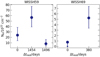 |
Fig. C.1. Intrinsic column density as a function of rest-frame time interval for the WISSH QSOs with multiple X-ray observations exhibiting > 2σ NH variability. |
WISSH QSOs with multiple X-ray observations showing > 2σ NH variability.
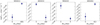 |
Fig. C.2. 0.5 − 2 keV flux as a function of rest-frame time interval for the four WISSH QSOs with multiple X-ray observations exhibiting > 3σ F0.5 − 2 variability. |
WISSH QSOs with multiple X-ray observations showing > 3σ F0.5 − 2 variability.
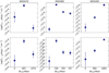 |
Fig. C.3. 0.5 − 2 keV (top panels) and 2 − 10 keV (bottom panels) flux as a function of rest-frame time interval for the three WISSH QSOs with multiple X-ray observations exhibiting > 3σ F0.5 − 2 and F2 − 10 variability. |
WISSH QSOs with multiple X-ray observations showing > 3σ F0.5 − 2 and F2 − 10 variability.
Appendix D: Corner plots for the best fit parameters
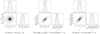 |
Fig. D.1. Corner plot of the best fit parameters in Sections 4.5 and 4.6. The correlation parameters are reported in Table D.1. The blue, green, and red contours show the 1σ, 2σ, and 3σ confidence level, respectively. |
Correlation parameters of the best fit relations in Sections 4.5 and 4.6.
Appendix E: Summary of the results
λL6 μm, kbol, αOX and Δ(αOX) for each QSO in the WISSH sample.
All Tables
WISSH QSOs with multiple X-ray observations showing > 3σ F0.5 − 2 variability.
WISSH QSOs with multiple X-ray observations showing > 3σ F0.5 − 2 and F2 − 10 variability.
All Figures
|
Fig. 1. X-ray coverage of the WISSH sample. |
| In the text | |
|
Fig. 2. (a) Chandra spectrum (re-binned for display purposes) of WISSH47 (z = 2.6987). We detect about 130 counts for this source and measure significant intrinsic absorption. The residuals are defined as (data – model) in units of σ. (b) NH − Γ contour plot for the best fit model of WISSH47. The blue, green, and red curves represent the 68%, 90%, and 99% confidence levels, respectively. |
| In the text | |
|
Fig. 3. Intrinsic column density distribution for the HC-WISSH sample. Sources for which the power law model represents the best fit (i.e. unobscured) are included in the bin NH < 5 × 1021 cm−2. |
| In the text | |
|
Fig. 4. Log(L2 − 10) as a function of Lbol for the entire WISSH sample. |
| In the text | |
|
Fig. 5. Bolometric correction as a function of Log(Lbol). WISSH BAL and non-BAL QSOs are shown as indigo and purple stars, respectively. The XMM-COSMOS sample of 343 Type 1 AGN presented by L10 is represented by yellow dots; it covers a wide range of redshifts (0.04 < z < 4.25) and X-ray luminosities (40.6 ≤ Log(L2 − 10/erg s−1)≤45.3). The 22 SUBWAYS QSOs and Type 1 AGN at intermediate redshifts (0.1 ≲ z ≲ 0.4) from Matzeu et al. (2023) can be seen as red dots. Light blue triangles correspond to the 14 radio-quiet high-λEdd (λEdd ≳ 1) QSOs at 0.4 ≤ z ≤ 0.75 presented by Laurenti et al. (2022). The sample of luminous and intrinsically blue QSOs at z ≈ 3 presented by Trefoloni et al. (2023), for which constrained L2 − 10, Γ, λEdd, and CIV line velocity values are available, are shown as pink squares. The black solid and dashed lines correspond to D20 best fit to Type 1 sources and its 0.26 dex spread, respectively. |
| In the text | |
|
Fig. 6. (a) Ratio of measured kbol values to expected kbol values from D20 as a function of Log(Lbol). WISSH QSOs are compared to literature samples; the symbols are the same as in Figure 5. The two black dashed lines correspond to the 0.26 dex spread of D20 best fit to Type 1 sources. (b) Distribution of WISSH QSOs kbol with respect to the D20 relation, including its spread (black horizontal dashed lines), i.e. being below, within, or above it. BAL and non-BAL sources are represented as indigo and purple bars, respectively. |
| In the text | |
|
Fig. 7. X-ray–to–optical index (αOX) as a function of Log(L2500#x2004;Å). WISSH QSOs are compared to literature samples; the symbols are the same as in Figure 5. The black dashed, solid, and dotted lines are the best fits from Martocchia et al. (2017), L10, and Just et al. (2007), respectively. In particular, L10 fit XMM-COSMOS data only; Just et al. (2007) consider 34 QSOs of their core sample, 332 sources from Steffen et al. (2006), and 14 from Shemmer et al. (2006); and Martocchia et al. (2017) consider XMM-COSMOS objects, 23 optically selected QSOs from the Palomar-Green (PG) Bright QSO Survey of the complete sample by Laor et al. (1994) and the 41 WISSH QSOs with available X-ray data at the time of the publication. |
| In the text | |
|
Fig. 8. Δ(αOX) = αOX − αOX, L10 distribution. αOX, L10 refers to the value derived from the L10 relation at a given L2500 Å. The BAL and non-BAL QSOs are represented as indigo and purple bars, respectively. The grey bar is for undetected sources, which have all been included in the X-ray-weakest bin. The grey-shaded area highlights the locus of X-ray-weak sources. |
| In the text | |
|
Fig. 9. X-ray photon index as a function of Δ(αOX) for the sources with ≥20 counts. (a) Γobs derived using a power law model modified by Galactic absorption. (b) Cold absorption component included in the spectral model used to derive Γ (see Section 3.1.1). The BAL and non-BAL QSOs are represented as indigo and purple dots, respectively. The grey-shaded areas highlight the locus of X-ray-weak sources. |
| In the text | |
|
Fig. 10. X-ray photon index as a function of Log(λEdd). Only WISSH QSOs with ≥20 photons (i.e. with X-ray spectral analysis), for which an estimate of MBH is available are considered. The symbols are the same as in Figure 5, with the exception of WISSH sources, which are represented as blue stars. The black solid, dashed, dotted, and dash-dotted lines correspond to the Liu et al. (2021) and Brightman et al. (2013) relations, and two models (BCES bisector and FITEXY method) from Trakhtenbrot et al. (2017), respectively. Specifically, Liu et al. (2021) consider 47 AGN with both super- and sub-Eddington accretion rates from the sample compiled by the SEAMBH collaboration (Du et al. 2018). Brightman et al. (2013) use 69 broad-line AGN from the extended Chandra Deep Field South and COSMOS surveys. Trakhtenbrot et al. (2017) refer to 228 hard X-ray selected AGN at 0.01 < z < 0.5, drawn from the Swift/BAT AGN Spectroscopic Survey (BASS, Baumgartner et al. 2013). |
| In the text | |
|
Fig. 11. Intrinsic column density (derived assuming Γ = 1.8) as a function of Log(λEdd). QSOs from the HC-WISSH sample with available MBH are plotted. WISSH BAL objects are contoured with a turquoise line. X-ray-weak QSOs (Δ(αOX) < − 0.2) are surrounded with a green circle. Blue and red QSOs are shown in the corresponding colour. Stars correspond to sources for which intrinsic absorption is significantly detected (see Sections 3.1.1 and 3.1.2). QSOs from Ricci et al. (2017) are shown as grey crosses. Black solid and dashed lines are Ishibashi et al. (2018) and Fabian et al. (2008) relations, derived from a maximal- and no-photon trapping model, respectively. The black horizontal dotted line indicates NH = 1022 cm−2. |
| In the text | |
|
Fig. 12. (a) Intrinsic 2 − 10 keV luminosity as a function of λL6 μm. WISSH BAL and non-BAL objects are shown as indigo and purple stars, respectively, while the grey dots represent various comparison samples from Lanzuisi et al. (2009), Mateos et al. (2015), and S15. The black solid, dashed, and dotted lines correspond to the relation by S15, Lanzuisi et al. (2009), and Chen et al. (2017), respectively; (b) Δ(αOX) as a function of the L2 − 10 offset of WISSH QSOs from the relation by S15 (Δ6 μm, X). WISSH BAL and non-BAL objects are indigo and purple dots, respectively. The grey-shaded area highlights the X-ray-weak region of the plane. The dispersion around the best fit (solid red line) is given by plotting ≈200 realisations considering the values of slope and intercept within 1σ of the sampled marginalised posterior distribution. |
| In the text | |
|
Fig. 13. Intrinsic 2 − 10 keV luminosity (top panel) and Δ(αOX) (bottom panel) as a function of CIV velocity vCIV. WISSH non-BAL objects are shown as purple dots. The dispersion around the best fits (solid red lines) is given by plotting ≈200 realisations considering the values of slope and intercept within 1σ of the sampled marginalised posterior distribution (see Figures D.1b and D.1c, and Table D.1 for further details). |
| In the text | |
|
Fig. 14. (a) Intrinsic 2 − 10 keV luminosity, (b) kbol/kbol, D20, and (c) photon index distributions. The histograms show the comparison between WISSH sources with ≥20 counts (green) and a sample of QSOs at z > 6 from Tortosa et al. (2024) (orange). |
| In the text | |
|
Fig. C.1. Intrinsic column density as a function of rest-frame time interval for the WISSH QSOs with multiple X-ray observations exhibiting > 2σ NH variability. |
| In the text | |
|
Fig. C.2. 0.5 − 2 keV flux as a function of rest-frame time interval for the four WISSH QSOs with multiple X-ray observations exhibiting > 3σ F0.5 − 2 variability. |
| In the text | |
|
Fig. C.3. 0.5 − 2 keV (top panels) and 2 − 10 keV (bottom panels) flux as a function of rest-frame time interval for the three WISSH QSOs with multiple X-ray observations exhibiting > 3σ F0.5 − 2 and F2 − 10 variability. |
| In the text | |
|
Fig. D.1. Corner plot of the best fit parameters in Sections 4.5 and 4.6. The correlation parameters are reported in Table D.1. The blue, green, and red contours show the 1σ, 2σ, and 3σ confidence level, respectively. |
| In the text | |
Current usage metrics show cumulative count of Article Views (full-text article views including HTML views, PDF and ePub downloads, according to the available data) and Abstracts Views on Vision4Press platform.
Data correspond to usage on the plateform after 2015. The current usage metrics is available 48-96 hours after online publication and is updated daily on week days.
Initial download of the metrics may take a while.