| Issue |
A&A
Volume 702, October 2025
|
|
|---|---|---|
| Article Number | A167 | |
| Number of page(s) | 12 | |
| Section | The Sun and the Heliosphere | |
| DOI | https://doi.org/10.1051/0004-6361/202555104 | |
| Published online | 24 October 2025 | |
Solar models with protosolar accretion and turbulent mixing
1
Department of Physics, Kurume University, 67 Asahimachi, Kurume, Fukuoka, 830-0011
Japan
2
Université Côte d’Azur, Observatoire de la Côte d’Azur, CNRS, Laboratoire Lagrange, Bd de l’Observatoire, CS 34229, 06304
Nice cedex 4, France
3
STAR Institute, Université de Liège, Liège, Belgium
⋆ Corresponding author: This email address is being protected from spambots. You need JavaScript enabled to view it.
Received:
10
April
2025
Accepted:
21
August
2025
Abstract
Context. Over the last two decades, no standard solar model (SSM) has been able to reproduce all observational data, resulting in active discussions regarding the so-called solar modeling problem. A recent study suggests that the accretion from the protosolar disk onto the proto-Sun could have left a large compositional gradient in the solar interior, in agreement with the low-metallicity (Z) solar surface and the high-Z solar core suggested by spectroscopic and neutrino observations, respectively. In addition, recent analyses have reported low lithium but high beryllium abundances on the solar surface; SSMs predict Li abundances that differ by ∼30σ from the observed value.
Aims. We develop solar models and compare them with the Li and Be abundance constraints.
Methods. We examined the effect of accretion and turbulent mixing below the base of the surface convective zone. We computed ∼200 solar evolutionary models for each case using target quantities to optimize input parameters, similar to the SSM framework.
Results. We confirm that turbulent mixing helps reproduce the surface Li and Be abundances within ∼0.6σ by boosting burning. This suppresses gravitational settling, leading to a better matching of the He surface abundance (≲0.3σ) and a smaller compositional gradient. We derive a new protosolar helium abundance, Yproto = 0.2651 ± 0.0035. Turbulent mixing decreases the central metallicity (Zcenter) by ≈4.4%; meanwhile, our previous study suggests that accretion increases Zcenter by essentially the same percentage. Unfortunately, the reduction in Zcenter implies that our models do not reproduce constraints on observed neutrino fluxes, with differences of 6.2σ for 8B and 2.7σ for CNO.
Conclusions. Including turbulent mixing in solar models appears indispensable to reproducing the observed atmospheric abundances of Li and Be. However, the resulting tensions in terms of neutrino fluxes, even in the models with protosolar accretion, show that the solar modeling problem remains, at least partly. We suggest that improved electron screening, as well as other microscopic properties, may help alleviate this problem. An independent confirmation of the neutrino fluxes as measured by the Borexino experiment would also be extremely valuable.
Key words: accretion / accretion disks / neutrinos / Sun: evolution / Sun: interior / Sun: abundances / protoplanetary disks
© The Authors 2025
 Open Access article, published by EDP Sciences, under the terms of the Creative Commons Attribution License (https://creativecommons.org/licenses/by/4.0), which permits unrestricted use, distribution, and reproduction in any medium, provided the original work is properly cited.
This article is published in open access under the Subscribe to Open model. This email address is being protected from spambots. You need JavaScript enabled to view it. to support open access publication.
1. Introduction
The Sun is a benchmark star for stellar structure and evolution theory. Much effort has been put into spectroscopic, helioseismic, and neutrino observations, resulting in constraints that have been used to test theoretical models. Over the last two decades, standard solar models (SSMs; Christensen-Dalsgaard et al. 1996), which are solar models constructed with standard input physics, have not been able to reproduce the surface metallicity (Zsurf), sound speed profile, and neutrino fluxes simultaneously (Vinyoles et al. 2017; Buldgen et al. 2019; Christensen-Dalsgaard 2021). This so-called solar modeling problem (or solar abundance problem) has been actively discussed in the community, with a clear solution yet to be found.
Concerning the solar modeling problem, two processes have drawn attention. The fit to the helioseismic constraints of the sound speed (cs) profile at the base of the surface convective zone (BCZ) can be significantly improved by an increase in opacity of ∼10% (e.g., Christensen-Dalsgaard et al. 2009; Villante 2010; Bailey et al. 2015; Buldgen et al. 2019; Kunitomo & Guillot 2021). In addition, the proto-Sun grew via accretion from the protosolar disk, where the planets were formed, but SSMs do not include the protosolar phase. Planet formation theory predicts that dust grains drift rapidly in the disk, and thus the dust-to-gas ratio (i.e., metallicity) of the accretion flow onto the proto-Sun must have been variable (see Kunitomo & Guillot 2021, hereafter KG21). The variable metallicity of accretion (Zaccretion; in particular, the low metallicity of the final phases of accretion) implies that the metallicity of the proto-Sun and thus the central metallicity (Zcenter) of the present-day Sun are higher than usually assumed (KG21). The higher Zcenter affects the thermal structure of the solar core and, thus, its neutrino fluxes. Kunitomo et al. (2022, hereafter KGB22) demonstrated for the first time that the models that include an ad hoc opacity increase and a variable Zaccretion reproduce all three constraints (Zsurf, cs, and neutrinos) simultaneously.
The abundance of light elements (i.e., lithium and beryllium) has been the subject of several recent studies (Amard et al. 2016; Eggenberger et al. 2022; Buldgen et al. 2025a; Yang et al. 2025). These elements are burned at relatively low temperatures, ∼2.5 million K (MK hereafter) for Li and ∼3.5 MK for Be, and thus their abundances are tied to internal mixing process. Comparisons to the meteoritic constraints for the Solar System primordial abundances (A(7Li) = 3.27 ± 0.03 dex and A(9Be) = 1.31 ± 0.04 dex; Lodders 2021)1 indicate that, at the surface of the present-day Sun, Li is depleted by > 2 dex (A(7Li)⊙ = 0.96 dex; Wang et al. 2021, see Table 1) whereas Be is only slightly depleted, by ∼0.1 dex (A(9Be)⊙ = 1.21 dex; Amarsi et al. 2024). Thus, in the solar interior, a mixing process must operate beyond the Li-burning region (≲0.65 R⊙) but should not reach the Be-burning region (∼0.55 R⊙).
Observational constraints of the present-day Sun.
Eggenberger et al. (2022) have shown that the Li abundance and rotation profile can be reproduced by rotational mixing, namely rotation-induced hydrodynamic and magnetohydrodynamic instabilities such as circulation, shear mixing, and magnetic Tayler instabilities (see also Buldgen et al. 2024). This is not the case for SSMs, which predict a value that differs by 30σ from the observed A(7Li)⊙ (see Fig. 6 of Eggenberger et al. 2022). However, the rotational mixing in Eggenberger et al. (2022) is too deep to reproduce A(9Be)⊙. Yang et al. (2025) examined another implementation of rotational mixing but were unable to reproduce the latest values of A(7Li)⊙ and A(9Be)⊙ simultaneously (Wang et al. 2021; Amarsi et al. 2024). Instead, a more localized shallow turbulent mixing is preferred (Buldgen et al. 2025a).
Therefore, the question of the present article is: If we consider protosolar accretion, an increase in the interior opacities, and turbulent mixing, can we reproduce Zsurf, cs, neutrino fluxes, and the Li and Be abundances simultaneously? This paper is organized as follows: we describe the computation method in Sect. 2, present the results in Sect. 3 (the evolution of surface Li and Be abundances, the metallicity profile at the solar age, and neutrino fluxes), discuss the origin of turbulent mixing and various effects on neutrino fluxes in Sect. 4, and summarize our results in Sect. 5.
2. Model
We simulated solar models with the Modules for Experiments in Stellar Astrophysics (MESA) stellar evolution code (version 12115), including the effects of protosolar accretion and turbulent mixing. For details, we refer the reader to the Paxton et al. papers and our previous papers (Kunitomo et al. 2017, 2018, KG21, and KGB22). Below, we summarize the computational method and the updates in this study. We mainly focus on protosolar accretion, turbulent mixing, opacity increase, abundance scale, and optimization.
Figure 1 illustrates two crucial physical processes of this paper, namely protosolar accretion with variable composition and turbulent mixing in the radiative zone. The proto-Sun grew by accretion from the protosolar disk, where planets were formed. Planets were formed by the coagulation of dust grains in the disk. Once the dust grains became centimeter-sized, which are called pebbles, they rapidly migrated onto the proto-Sun due to the frictional force with the disk gas. This led to an increase in the metallicity of the accreted gas, Zaccretion. We call this the “pebble wave phenomenon”. In contrast, in the late phase, the disk gas became depleted in heavy elements (i.e., metals) due to the drift or the filtration by proto-giant planets (Guillot et al. 2014). Thus, a variable composition of the accreted gas is a natural consequence of recent planet formation theory (see KG21 and references therein). We also computed models with steady Zaccretion (i.e., constant primordial metallicity, Zproto, over time), which correspond to the cases with no planet formationprocesses.
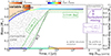 |
Fig. 1. Schematic illustration showing the structure evolution (panel a; the so-called Kippenhahn diagram) and the Dmix profile at the solar age (panel b) of our fiducial model, K2-MZvar-TM (see Table 2). The convective zones are depicted as a cloudy region. The color of the shade in panel a shows Zaccretion. The two lines at the stellar surface and center illustrate metallicity by color. The two dashed green lines the locations at temperatures 2.5 × 10⁶ and 3.5 × 10⁶ K, indicative of Li and Be burning, respectively. |
We adopted a Zaccretion model following KG21 (see their Fig. 4): Zaccretion = Zproto in the earliest phase (until stellar mass, M⋆, reaches M1), Zaccretion increases up to Zacc,max during the pebble-wave phase (M1 < M⋆ < M2), and then Zaccretion = 0 in the late phase. For simplicity, in the models with variable Zaccretion, we adopted M1, M2, and Zacc,max values from the best model in KG21, K2-MZvar-A2-12 (M1 = 0.90 M⊙, M2 = 0.96 M⊙, and Zacc,max = 0.065; see their Table A.1). Simulations start with a 0.1 M⊙ seed, mass accretion rate, Ṁacc, decreases with time following Hartmann et al. (1998), and accretion stops at 10 Myr (see Fig. 3 of KG21).
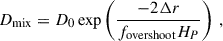
For turbulent mixing, we followed Proffitt & Michaud (1991) and Buldgen et al. (2025a); thus, the diffusion coefficient in the radiative core in the main sequence (MS) is given by
 (1)
(1)
where ρ is the density, r is the radius, RCZ is the radius at the BCZ, DT is the diffusion coefficient at the BCZ, and n is a power-law index. We turned on mixing at 30 Myr2. Buldgen et al. (2025a, see their Table 3) investigated a wide range of n and DT sets and found that A(7Li)⊙ and A(9Be)⊙ can be well reproduced if n ∼ 3 − 6 and DT ∼ 3000 − 10 000 cm2/s. In this study we adopted n = 4 and DT = 5000 cm2/s for the models that include mixing.
As for the other internal mixing processes, convection is treated by the mixing-length theory (Cox & Giuli 1968). Overshooting is not considered except for the K2-fov models, as in KG21 and KGB22 (see Appendix B). Gravitational setting is included (Thoul et al. 1994)3. Radiative levitation is not considered.
The opacity in the solar BCZ condition remains uncertain and is actively discussed. As in KG21, we considered opacity increase at around the BCZ as
 (2)
(2)
where4
![Mathematical equation: $$ \begin{aligned} \delta _\kappa = A_2\,\exp \left[ -\frac{ \left( \log (T/\mathrm{K}) -b_2\right)^2}{2c_2^2} \right]. \end{aligned} $$](/articles/aa/full_html/2025/10/aa55104-25/aa55104-25-eq8.gif) (3)
(3)
We adopted b2 = 6.45 and c2 = 0.18 (Le Pennec et al. 2015; see also Fig. A.1), and T is the temperature. We determined the free parameter A2 to be 10% from a parameter study with the K2-A2 models and adopted this value for all other models. We note that this value is similar to 12% used in KG21 and KGB22 (see Appendix A), and close to the suggestions by experiments (4–10%; Bailey et al. 2015) and helioseismic analyses (∼10% at ∼2 MK; Buldgen et al. 2025b). We refer the reader to KG21 and references therein for more details.
In this study we adopted the solar abundance scale in Asplund et al. (2021, hereafter AAG21) instead of the Asplund et al. (2009, hereafter AGSS09) scale used by KG21 and KGB22. Therefore, we used the different target (Z/X)surf value, corresponding opacity tables, A2 value, and initial seed, from KG21 and KGB22 (see Table 1 and Appendix A for more details).
Table 2 summarizes the settings of the simulation models under a variety of settings (e.g., with and without turbulent mixing, variable or steady Zaccretion). We optimized input parameters using the downhill simplex method (Nelder & Mead 1965). In this study, we used (Z/X)surf, L⋆, and Teff (surface abundance ratio of metals to hydrogen, luminosity, and effective temperature, respectively; see Table 1) as target values in order to iteratively calibrate αMLT, Yproto, and Zproto (mixing-length parameter, primordial helium abundance, and primordial metallicity, respectively). Thus, N = M = 3, where N and M are the numbers of target values and input parameters, respectively. In optimization, the reduced χ2 value with N = 3 is minimized (see Eq. (8) of KG21). When we examined the quality of the solution, we also calculated χ2N = 6 by adding the surface helium abundance Ysurf, the location of the convective-radiative boundary RCZ, and root-mean-square sound speed rms(δcs) (see Fig. A.1), or χ2N = 8 by further adding the surface Li abundance A(7Li), and the surface Be abundance A(9Be) (see Table C.2).
Settings of optimization simulations.
3. Results
In this section we show the evolutions of surface He, Li, and Be abundances, the metallicity profile, and neutrino fluxes, focusing on the models K2-MZvar-TM, K2-MZvar, K2-TM, and K2 (see Table 2).
Figure 2 shows the evolutions of Ysurf, surface A(7Li), and surface A(9Be). The models with turbulent mixing (K2-TM and K2-MZvar-TM; solid lines) reproduce the three observations within 0.6σ, as in Buldgen et al. (2025a). The gradual depletion of the A(7Li) values of solar-type stars (Carlos et al. 2019; Dumont et al. 2021, and references therein) is also well reproduced by the models with the mixing. In models without turbulent mixing (K2 and K2-MZvar; dashed lines), helium settling is too efficient and the observed Ysurf is not well reproduced (1.4σ and 1.2σ, respectively). Li and Be are not burned and thus their abundances are too high at the solar age (∼30σ and ∼2σ, respectively). In these models, the slight decreases in A(7Li) and A(9Be) are driven by gravitational settling, not nuclear burning. Because He, Li, and Be depletion occurs in the MS, this behavior is independent of the protosolar accretion history.
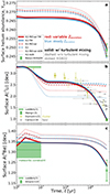 |
Fig. 2. Evolution of the surface abundances of helium (panel a), lithium (b), and beryllium (c). The red and blue lines show the models with variable and steady Zaccretion, respectively. The solid and dashed lines show the models with and without turbulent mixing, respectively. The dotted lines show the models from KGB22 (with AGSS09 abundances, without turbulent mixing but with overshooting). See Table 2 for more details. The green points show the observational constraints of the present-day Sun (see Table 1). The green shades show the meteoritic constraints (Lodders 2021) arbitrarily extending from 1 to 10 Myr. The crosses and small circles in panel b show the observed A(7Li) values of clusters (Dumont et al. 2021) and individual stars (Carlos et al. 2019), respectively, that are younger than the Sun. |
Lithium is depleted by ∼0.6 dex from 3 to 15 Myr. This is because the temperature at the BCZ exceeds 2.5 MK (see Fig. 1a), and thus Li is burned (but limited due to the short timescale; see also Eggenberger et al. 2022; Buldgen et al. 2023). The best models of KGB22 (dotted lines) deplete Li more (up to ∼1.3 dex) in the pre-MS because they include overshooting (see Appendix B).
We note the variety in the initial Li and Be abundances. In the calibration procedure (see Sect. 2), the primordial metallicity Zproto is treated as a free parameter. Since we adopted the abundance scale of AAG21, the initial Li and Be abundances were also adjusted accordingly during the calibration. Nevertheless, the initial A(7Li) and A(9Be) in the models with turbulent mixing agree with the meteoritic constraints provided by Lodders (2021).
Figure 3 shows the present-day metallicity profile. The turbulent mixing is apparent below the BCZ: the metallicity jumps at the BCZ in the models without it because of gravitational settling, whereas turbulent mixing smooths the metallicity profile down to ∼0.5 R⊙. This corresponds to the extent from the BCZ (= 0.713 R⊙) reached by diffusion by the solar age. The diffusion timescale tmix at a scale Δr is estimated as
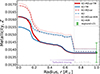 |
Fig. 3. Solar metallicity profile at the present day of the six models shown in Fig. 2. The dashed vertical line shows the BCZ. See Fig. B.2 for the Dmix profile. |
 (4)
(4)
The central metallicity, Zcenter, is also lower because gravitational settling is suppressed. In models with variable and steady Zaccretion, the turbulent mixing decreases Zcenter by 4.4% and 4.3%, respectively. The finding in KG21, that is, variable Zaccretion can increase Zcenter by up to ∼5%, is still valid even for the models with turbulent mixing (4.4%). Therefore, the effects of variable Zaccretion and turbulent mixing are counterbalanced: the model with turbulent mixing and variable Zaccretion has almost the same Zcenter as the model with steady Zaccretion withoutmixing.
The lower Zcenter due to turbulent mixing directly impacts neutrino fluxes. Figure 4 shows that the new models with turbulent mixing (orange points) do not reproduce the observed neutrino fluxes. Their Φ(8B) and Φ(7Be) are lower than for themodels without turbulent mixing (brown) and for the observations. These fluxes are strongly sensitive to the central temperature Tcenter ( and
and  ; Bahcall & Ulmer 1996); thus, the lower fluxes come from the lower Tcenter. There are two reasons for the lower Tcenter: the lower Zcenter due to the fact that mixing reduces the central opacity and Tcenter as well. In addition, turbulent mixing suppresses helium settling, leading to a lower mean molecular weight at the center, μcenter. For the hydrostatic equilibrium (pressure ∝ Tρ/μ), this leads to the lower Tcenter.
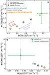 |
Fig. 4. Solar neutrino fluxes. The stars and circles show the models with variable and steady Zaccretion, respectively. Orange and brown illustrate the models with and without turbulent mixing, respectively. Blue shows the models from KGB22 (with AGSS09 abundances and without turbulent mixing). The points with error bars are the observational constraints (Table 1). The dotted cyan error bar shows an old constraint from Borexino Collaboration (2020). |
Figure 4b shows that turbulent mixing reduces Φ(CNO). This flux is also highly sensitive to both Tcenter and Zcenter. Both a lower Tcenter and a lower Zcenter lead to a lower Φ(CNO) in the models with mixing. By contrast, the Φ(pp) is higher. This flux depends on Xcenter2, where Xcenter is the central hydrogen abundance. Because of inefficient helium settling, Xcenter is higher. We note that the lower Tcenter is counterbalanced by a higher Xcenter and thus the observed luminosity, L⊙, is well reproduced. As a result, the neutrino fluxes of model K2-TM (with mixing and steady Zaccretion; orange circle in Fig. 4) are far from the observations: Φ(8B), Φ(7Be)), Φ(pp), and Φ(CNO) are within 7.9σ, 1.5σ, 1.8σ, and 3.1σ.
KGB22 find that a higher Zcenter due to variable Zaccretion leads to higher neutrino fluxes, matching the observations. The fluxes of our fiducial model with turbulent mixing with variable Zaccretion (K2-MZvar-TM; orange star) are indeed closer to observations compared to K2-TM. Thus, the fact that a higher Zcenter due to variable Zaccretion leads to higher neutrino fluxes remains valid in the models with turbulent mixing. However, the effect of accretion is not sufficient: model K2-MZvar-TM is distant from the observations by 6.2σ for Φ(8B), 1.2σ for Φ(7Be), 1.6σ for Φ(pp), and 2.7σ for Φ(CNO). In particular, Φ(8B) and Φ(CNO) still poorly match observations. Therefore, we conclude that, although variable Zaccretion is still a key process to explain the neutrino fluxes, we need another physical process (Sect. 4) to reproduce at the same time the light element abundances, A(7Li)⊙ and A(9Be)⊙, and the neutrino fluxes.
Here we explain why the models in KGB22 (blue) have higher Φ(8B) and Φ(7Be) than the new models without mixing (brown) even though these models have similar Zcenter (Fig. 3). This results from a higher Tcenter in the KGB22 models, which is caused by a higher μcenter. The increase in μcenter originates from a higher central helium abundance Ycenter, which in turn results from the extended calibration: KGB22 adopted six input parameters (N = 6), including Ysurf. Since the KGB22 models do not include turbulent mixing, gravitational helium settling is efficient. To match the observed Ysurf, the initial abundance Yproto has to be higher (see Fig. 2a), and thus the bulk Y and Ycenter are also higher. From the comparison with the models with N = 3 and AGSS09 abundances, we confirmed this calibration effect: these models with steady or variable Zaccretion have slightly lower Ycenter, Φ(8B), and Φ(7Be) values than models K2 or K2-MZvar.
4. Discussions
4.1. Origin of turbulent mixing
It has been noted since the 1990s that turbulent mixing at the BCZ is missing from the SSMs (Christensen-Dalsgaard et al. 1996). Its exact physical origin is yet unknown, as the BCZ is the place of multiple physical phenomena that could lead to additional mixing of chemicals. Brun et al. (2002) link thismixing to the presence of the solar tachocline, which coincides with the BCZ. More recently, Eggenberger et al. (2022) constructed solar models including circulation, shear instability, and magnetic Tayler instability. These models could be calibrated to reproduce the Li depletion observed in the Sun. However, the revision of the Be abundance (Amarsi et al. 2024) showed that only a small amount of Be was burned at the solar age, implying a shallow depth of turbulent mixing at the BCZ. This was shown to be in disagreement with models including the effects of rotation (Buldgen et al. 2024, 2025a), as models including circulation, shear instability, and magnetic Tayler instability present an extended mixed region down to ∼0.4 R⊙, while observations of Be forbid a mixing below ∼0.6 R⊙. It is unclear yet whether the depletion of Li and Be is directly linked to the flat rotation profile in the solar radiative interior (down to ∼0.2 R⊙; Couvidat et al. 2003) and there is no consensus on the underlying physical mechanism responsible for angular momentum transport in the solar interior.
One might think that overshooting is the origin of the mixing below the BCZ. KGB22 adopted diffusive overshooting, which enhances Li depletion in the pre-MS phase (Sect. 3). Indeed, with a more efficient diffusive overshooting, A(7Li)⊙ can be reproduced (Fig. B.1b). However, the observed gradual decrease in the surface A(7Li) of solar-type stars cannot be reproduced, and a slight decrease in A(9Be) from the protosolar phase to the present-day, which observations suggest, is also not made. We discuss the effect of diffusive overshooting in Appendix B in more detail.
Although the diffusive overshooting model (Herwig 2000) is widely used, other overshooting models have also been discussed. Zhang et al. (2019) suggested that the inclusion of an overshooting model could solve the sound speed discrepancies and the Li depletion. However, while the sound speed can be corrected, the model of Zhang et al. (2019) does not allow us to correct the density profile in the convective envelope (see model OV09Ne in their Fig. 1). Recent works by Baraffe et al. (2021) and Baraffe et al. (2022) have shown that convective penetration is not expected to fully correct the sound speed anomaly and extend deep enough to burn both Li and Be based on multidimensional hydrodynamic simulations. Zhang et al. (2023) have suggested another overshooting model and tested it on asteroseismic observations of a B-type star. The application of this new model to the case of the base of the solar convective envelope could have an impact on the depletion of Li and Be.
4.2. Solar evolutionary models with rotation
In this study we considered turbulent mixing below the BCZ (Proffitt & Michaud 1991; Buldgen et al. 2025a, see Sect. 2). Although this is likely to be related to rotational mixing, the exact underlying process is still under debate (Sect. 4.1). In this study, we did not solve angular momentum evolution and instead adopted an empirical mixing model in nonrotating solar models. In addition to the physical origin of the mixing, there is also a practical numerical issue in the treatment of meridional circulation. In principle, the circulation should be calculated using an advective term in the angular momentum transport equation, and some stellar evolution codes follow this implementation, such as GENEC (Eggenberger et al. 2022), Cesam2k20 (Marques et al. 2013; Manchon et al., in preparation), and STAREVOL (Palacios et al. 2006; Decressin et al. 2009). However, due to numerical difficulties, others, such as MESA (Paxton et al. 2013), PARSEC (Nguyen et al. 2022), and YREC (Yang et al. 2025), treat circulation as a diffusion term (see discussions in Potter et al. 2012; Salaris & Cassisi 2017). In the future, rotating solar models should be developed and reproduce self-consistently all the solar observations (i.e., (Z/X)surf, cs profile, neutrino fluxes, Li and Be abundances, and rotation profile; Eggenberger et al. 2022), as well as be consistent with asteroseismic constraints on the internal rotation (e.g., Buldgen & Eggenberger 2023; Dumont 2023).
Regarding rotational mixing, the initial rotation rate is a key parameter. The protoplanetary disk can regulate the rotation period of pre-MS stars via star-disk interaction (so-called disk-locking; see, e.g., Amard & Matt 2023; Takasao et al. 2025). The longer disk lifetime leads to a slow rotator, which may have a stronger shear in the interior and thus a more efficient Li depletion (Eggenberger et al. 2012). Also, the long disk lifetime is likely to lead to a higher chance of giant planet formation. Bouvier (2008) suggested a possible link between Li abundance and exoplanet occurrence rate. This link should be investigated in more detail in future work.
4.3. Li depletion by cold accretion
We note the effect of protostellar accretion on Li depletion. Accretion affects the thermal evolution of protostars (e.g., Hartmann et al. 1997; Kunitomo et al. 2017). Baraffe & Chabrier (2010) found that if the accretion entropy is quite low (so-called cold accretion scenario), the stellar interior is hot enough to quickly deplete Li in the accretion phase (see also Tognelli et al. 2020). However, Kunitomo et al. (2017) concluded from a comparison with young clusters on the Hertzsprung–Russell diagram that most stars should not have experienced cold accretion. Furthermore, again, this scenario does not explain the observed gradual decrease in A(7Li) of solar-type stars.
4.4. A new protosolar helium abundance
Figure 2a and Table C.1 show that the models with turbulent mixing that reproduce the constraints on the observed atmospheric abundances of lithium and beryllium have a protosolar helium abundance (Yproto) ranging from 0.2648 to 0.2659. Reporting the uncertainty on the present-day solar atmospheric helium abundance from Basu & Antia (2004) to the values above, we find a revised value Yproto = 0.2654 ± 0.0035. This is lower than the value derived from classical evolution models of the Sun, Yproto ∼ 0.278 ± 0.006 (Serenelli & Basu 2010).
Figure 5 demonstrates that turbulent mixing lowers the estimated Yproto value. Turbulent mixing suppresses gravitational helium settling, and thus model K2-MZvar-TM has a low Yproto value and successfully reproduces the present-day Ysurf constraint. Although the non-accreting model noacc-noov from KG21 that includes standard atomic diffusion (i.e., no overshooting and turbulent mixing) also reproduces Ysurf, this model has a high Yproto value5 within the range suggested by Serenelli & Basu (2010) and causes efficient helium settling.
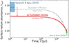 |
Fig. 5. Evolution of Ysurf in model K2-MZvar-TM (solid red line) and a non-accreting model from KG21 with standard atomic diffusion (i.e., no overshooting and with turbulent mixing; dashed gray) starting with a high Yproto value within the range suggested by Serenelli & Basu (2010, blue shaded region). Turbulent mixing suppresses gravitational settling and thus leads to a reduced Yproto value. |
While the inclusion of additional mixing at the BCZ leads to an incompatibility with neutrino fluxes (Sect. 4.5), they do reproduce the surface He, Li and Be abundances at the age of the Sun better than SSMs (see Fig. 2 and Table C.2). Therefore, it appears that our description of the efficiency of mixing at the BCZ is more realistic than that of SSMs. This implies that the value we provide for Yproto can be considered quite reliable but should be revised after any potential future improvements to the physical ingredients of solar models.
The constraint on Yproto from solar modeling is a key ingredient for interior models of Jupiter and Saturn (Guillot 2005): The precise determination of the masses and shapes of these planets (and therefore their mean density) implies that the bulk abundance of heavy elements (all elements other than hydrogen and helium) that is inferred to be present in the interiors of these planets is inversely correlated to Yproto. Recently, the precise measurements of the masses and gravitational moments by Juno in Jupiter (Iess et al. 2018) and Cassini in Saturn (Iess et al. 2019) have led to a decisive tightening of the constraints on interior models. This has resulted in tensions between a very low value of the enrichment in heavy elements in the outer envelopes of these planets, as favored by interior models, compared to atmospheric constraints from spectroscopy and in situ measurements that yield clear enrichments over solar values (see Mankovich & Fuller 2021; Howard et al. 2023; Guillot et al. 2023, and references therein).
Models of Jupiter and Saturn (e.g., Guillot et al. 2018) have so far relied on the constraint derived from classical evolution models of the Sun (Yproto ∼ 0.278 ± 0.006; see above), while our new value is lower by 0.0126, equivalent to a global enrichment in heavy elements by approximately one-time solar value. Using this revised value may help ease some of the tension between interior models and spectroscopy, although for Jupiter this effect will be limited by the fact that the helium abundance in the planet’s atmosphere has been precisely measured by the Galileo probe (von Zahn et al. 1998).
4.5. Explaining the neutrino fluxes
Our models with turbulent mixing have lower Φ(8B), Φ(7Be), and Φ(CNO) than the observed constraints, even in the case with variable Zaccretion (Fig. 4). We discuss hereafter several effects that might account for this disagreement: input physics (nuclear reactions, opacity, solar winds, and variable Zaccretion model) and observations’ uncertainties (particularly on CNO neutrinos).
Neutrino fluxes can be influenced by the ingredients of solar models, including the formalism used for electron screening, nuclear reaction rates, and opacities. Electron screening seems to be the most promising avenue; the current formalism applied in all stellar evolution codes is that of static screening, which neglects the velocity differences between electrons and ions. Recently, Däppen (2024) wrote a brief review of the current state of the issue, highlighting that this effect still needs to be studied in detail as it impacts core conditions and neutrino fluxes, potentially leading to higher central temperature and metallicity in calibrated solar models. Updated nuclear reaction rates have been recently published (Solar Fusion III; Acharya et al. 2024) and could slightly modify the values found by calibrated solar models. Regarding opacities, the physical origin of the observed differences between theoretical computations and the measurement of Bailey et al. (2015) and Nagayama et al. (2019) is still unknown, and measurements at higher temperatures and electron densities have not been achieved yet. Therefore, the measured differences cannot be reliably extrapolated to conditions deeper in the Sun, implying that the expected impact on the solar core conditions and the neutrino fluxes is yet unknown. All three effects remain potential progress avenues that would alter the comparisons between solar models and neutrino experiments.
Zhang et al. (2019, see their Fig. 18) showed showed that solar winds can increase Zcenter (see also Sackmann & Boothroyd 2003; Wood et al. 2018). Both observational and theoretical studies have suggested that the young Sun had more vigorous winds than presently (Wood et al. 2005; Suzuki et al. 2013). If solar winds are metal-rich (e.g., first ionization potential effect), then the metallicity gradient becomes larger with time. This scenario is interesting, but the history of mass-loss rate and composition evolution is still quite uncertain. This needs to be investigated in more detail in the future (Buldgen et al. 2025c).
The variable Zaccretion increases Φ(8B), Φ(7Be), and Φ(CNO). In this study we used the same Zaccretion model as in the best model of KGB22 (i.e., M1 = 0.90 M⊙, M2 = 0.96 M⊙, and Zacc,max = 0.065). This is determined by complex dust dynamics in the protosolar disk. Moreover, we fixed the abundance scale to AAG21 and changed the metallicity, but each element can behave differently. If we expand the model further to treat the abundance of each element in the accretion flow, the central CNO abundance (and thus CNO neutrino fluxes) may increase. An interdisciplinary study integrating knowledge from solar and stellar physics, planet formation theory, disk chemistry, and Solar-System studies will be needed in the future.
Finally, we note that although truly substantial efforts have been made on the observational side, the interpretation of the observed neutrino fluxes is still challenging. In particular, CNO neutrinos have been detected only in the Borexino experiment. We also note that the Φ(CNO) constraint has been updated: the new constraint (green circle in Fig. 4b; Basilico et al. 2023) is slightly lower than the previous one (cyan dotted error bar; Borexino Collaboration 2020,  ) but has a much smaller uncertainty. Both constraints were derived from the data of the Borexino experiments, but different analysis techniques were used. The best model in KGB22 agreed with the old constraint by 0.99σ, while the new constraint leads to a worse value of 2.11σ. The best model in this paper, K2-MZvar-TM, has 1.2σ and 2.7σ, respectively. Given the direct impact of a revision of the precision of the observational constraints on the conclusions drawn on solar models, an independent measurement of Φ(CNO) would be a strong confirmation of the current observed disagreements.
5. Conclusion
The structure and evolution of the Sun have usually been tested via comparisons with the observations of surface metallicity, helioseismic constraints, and neutrino fluxes. Our previous study, KGB22, showed that protosolar accretion can lead to an increase in the central metallicity by up to ≈5%, thus significantly improving the agreement between theoretical and measured neutrino fluxes. Since KGB22, recent refinements of the lithium and beryllium abundances on the solar surface have highlighted the importance of turbulent mixing in the solar interior. This led us to develop solar models that include both protosolar accretion and turbulent mixing to account for the measured surface Li and Be abundances.
Our models with turbulent mixing reproduce the observed He, Li, and Be abundances well, within 0.3σ, 0.6σ, and 0.5σ, respectively, consistent with previous studies (Buldgen et al. 2025a). This is a significant improvement from models without mixing, which reproduce them within ∼1.4σ, ∼30σ, and ∼2.0σ, respectively. The difference comes from two effects of the mixing: it promotes nuclear burning, thereby depleting Li and Be, and suppresses the gravitational settling of He. The models indicate a lower protosolar He abundance, Yproto = 0.2651 ± 0.0035, than previously suggested.
The limited settling due to turbulent mixing reduces the central metallicity, Zcenter, by ≈4.4%. This is essentially the same amount as that of the increase (≈4.4%) due to protosolar accretion with variable composition, as found by KG21. This leads to neutrino fluxes in disagreement with observations: for the model K2-TM with turbulent mixing and steady Zaccretion, by 7.9σ, 1.5σ, 1.8σ, and 3.1σ for Φ(8B), Φ(7Be), Φ(pp), and Φ(CNO). For the model K2-MZvar-TM with turbulent mixing and variable Zaccretion, the situation improves but remains insufficient: 6.2σ, 1.2σ, 1.6σ, and 2.7σ, respectively. Therefore, while variable Zaccretion remains an important effect to reproduce the observed neutrino fluxes, as it has a strong impact on the central metallicity, it is insufficient on its own.
Further investigations of the physical mechanisms responsible for internal mixing in the Sun are needed to understand the magnitude of turbulent mixing and its consequences for the Sun’s internal structure and evolution. Although they are likely related to rotation, Buldgen et al. (2025a) suggested the need for an improvement from the state-of-the-art model in Eggenberger et al. (2022). In our study we did not consider rotation but instead adopted an empirical turbulence model that treats it as a diffusion coefficient related to density, as in Proffitt & Michaud (1991) and Buldgen et al. (2025a), to model the transport of chemicals. The investigation of the underlying physics of the light element depletion observed in the Sun should ideally be coupled to the derivation of a self-consistent and physically motivated description of the evolution of angular momentum. The remaining neutrino flux differences between observations and our models that include both turbulent mixing and protosolar accretion likely require further examination of input physics such as electron screening, nuclear reaction rates, and the impact of solar winds, as well as the Zaccretion model itself (Buldgen et al. 2025c). Furthermore, a higher precision on the determination of neutrino fluxes, especially Φ(8B) and Φ(CNO), would greatly help in further constraining the physical ingredients of solar models.
Data availability
Tables C.1 and C.2 and supplemental materials are available on Zenodo at https://doi.org/10.5281/zenodo.16789192.
Acknowledgments
We thank the anonymous referee for helpful comments that improved this paper. We are also grateful to Ebraheem Farag for his valuable comments on MESA. M.K. thanks Observatoire de la Côte d’Azur for the hospitality during his long-term stay in Nice. This work was supported by JSPS KAKENHI Grant Nos. JP23K25923, JP24K07099, and JP24K00654. G.B. acknowledges fundings from the Fonds National de la Recherche Scientifique (FNRS) as a postdoctoral researcher. T.G. acknowledges funding from the Programme National de Planétologie. Numerical computations were carried out on the PC cluster at the Center for Computational Astrophysics, National Astronomical Observatory of Japan. Software: MESA (version 12115; Paxton et al. 2011, 2013, 2015, 2018, 2019).
References
- Acharya, B., Aliotta, M., Balantekin, A. B., et al. 2024, arXiv e-prints [arXiv:2405.06470] [Google Scholar]
- Amard, L., & Matt, S. P. 2023, A&A, 678, A7 [NASA ADS] [CrossRef] [EDP Sciences] [Google Scholar]
- Amard, L., Palacios, A., Charbonnel, C., Gallet, F., & Bouvier, J. 2016, A&A, 587, A105 [NASA ADS] [CrossRef] [EDP Sciences] [Google Scholar]
- Amarsi, A. M., Ogneva, D., Buldgen, G., et al. 2024, A&A, 690, A128 [NASA ADS] [CrossRef] [EDP Sciences] [Google Scholar]
- Amelin, Y., Krot, A. N., Hutcheon, I. D., & Ulyanov, A. A. 2002, Science, 297, 1678 [NASA ADS] [CrossRef] [Google Scholar]
- Asplund, M., Grevesse, N., Sauval, A. J., & Scott, P. 2009, ARA&A, 47, 481 [NASA ADS] [CrossRef] [Google Scholar]
- Asplund, M., Amarsi, A. M., & Grevesse, N. 2021, A&A, 653, A141 [NASA ADS] [CrossRef] [EDP Sciences] [Google Scholar]
- Bahcall, J. N., & Ulmer, A. 1996, Phys. Rev. D, 53, 4202 [NASA ADS] [CrossRef] [Google Scholar]
- Bahcall, J. N., Basu, S., Pinsonneault, M., & Serenelli, A. M. 2005, ApJ, 618, 1049 [NASA ADS] [CrossRef] [Google Scholar]
- Bailey, J. E., Nagayama, T., Loisel, G. P., et al. 2015, Nature, 517, 56 [NASA ADS] [CrossRef] [Google Scholar]
- Baraffe, I., & Chabrier, G. 2010, A&A, 521, A44 [NASA ADS] [CrossRef] [EDP Sciences] [Google Scholar]
- Baraffe, I., Pratt, J., Vlaykov, D. G., et al. 2021, A&A, 654, A126 [NASA ADS] [CrossRef] [EDP Sciences] [Google Scholar]
- Baraffe, I., Constantino, T., Clarke, J., et al. 2022, A&A, 659, A53 [NASA ADS] [CrossRef] [EDP Sciences] [Google Scholar]
- Basilico, D., Bellini, G., Benziger, J., et al. 2023, Phys. Rev. D, 108, 102005 [NASA ADS] [CrossRef] [Google Scholar]
- Basu, S., & Antia, H. M. 2004, ApJ, 606, L85 [CrossRef] [Google Scholar]
- Basu, S., Chaplin, W. J., Elsworth, Y., New, R., & Serenelli, A. M. 2009, ApJ, 699, 1403 [NASA ADS] [CrossRef] [Google Scholar]
- Borexino Collaboration (Agostini, M., et al.) 2020, Nature, 587, 577 [NASA ADS] [CrossRef] [Google Scholar]
- Bouvier, J. 2008, A&A, 489, L53 [Google Scholar]
- Brun, A. S., Antia, H. M., Chitre, S. M., & Zahn, J. P. 2002, A&A, 391, 725 [NASA ADS] [CrossRef] [EDP Sciences] [Google Scholar]
- Buldgen, G., & Eggenberger, P. 2023, in The Sixteenth Marcel Grossmann Meeting, eds. R. Ruffino, & G. Vereshchagin, On Recent Developments in Theoretical and Experimental General Relativity, Astrophysics, and Relativistic Field Theories, 2848 [Google Scholar]
- Buldgen, G., Salmon, S. J. A. J., Noels, A., et al. 2019, A&A, 621, A33 [NASA ADS] [CrossRef] [EDP Sciences] [Google Scholar]
- Buldgen, G., Eggenberger, P., Noels, A., et al. 2023, A&A, 669, L9 [NASA ADS] [CrossRef] [EDP Sciences] [Google Scholar]
- Buldgen, G., Noels, A., Scuflaire, R., et al. 2024, A&A, 686, A108 [NASA ADS] [CrossRef] [EDP Sciences] [Google Scholar]
- Buldgen, G., Noels, A., Amarsi, A. M., et al. 2025a, A&A, 694, A285 [NASA ADS] [CrossRef] [EDP Sciences] [Google Scholar]
- Buldgen, G., Pain, J.-C., Cossé, P., et al. 2025b, Nat. Commun., 16, 693 [Google Scholar]
- Buldgen, G., Canocchi, G., Le Saux, A., et al. 2025c, Sol. Phys., 300, 97 [Google Scholar]
- Carlos, M., Meléndez, J., Spina, L., et al. 2019, MNRAS, 485, 4052 [Google Scholar]
- Christensen-Dalsgaard, J. 2021, Liv. Rev. Sol. Phys., 18, 2 [NASA ADS] [CrossRef] [Google Scholar]
- Christensen-Dalsgaard, J., Dappen, W., Ajukov, S. V., et al. 1996, Science, 272, 1286 [Google Scholar]
- Christensen-Dalsgaard, J., di Mauro, M. P., Houdek, G., & Pijpers, F. 2009, A&A, 494, 205 [NASA ADS] [CrossRef] [EDP Sciences] [Google Scholar]
- Colgan, J., Kilcrease, D. P., Magee, N. H., et al. 2016, ApJ, 817, 116 [Google Scholar]
- Couvidat, S., García, R. A., Turck-Chièze, S., et al. 2003, ApJ, 597, L77 [Google Scholar]
- Cox, J., & Giuli, R. 1968, Principles of stellar structure (New York: Gordon and Breach), 401 [Google Scholar]
- Däppen, W. 2024, Sol. Phys., 299, 128 [Google Scholar]
- Decressin, T., Mathis, S., Palacios, A., et al. 2009, A&A, 495, 271 [NASA ADS] [CrossRef] [EDP Sciences] [Google Scholar]
- Dumont, T. 2023, A&A, 677, A119 [NASA ADS] [CrossRef] [EDP Sciences] [Google Scholar]
- Dumont, T., Palacios, A., Charbonnel, C., et al. 2021, A&A, 646, A48 [EDP Sciences] [Google Scholar]
- Eggenberger, P., Haemmerlé, L., Meynet, G., & Maeder, A. 2012, A&A, 539, A70 [NASA ADS] [CrossRef] [EDP Sciences] [Google Scholar]
- Eggenberger, P., Buldgen, G., Salmon, S. J. A. J., et al. 2022, Nat. Astron., 6, 788 [NASA ADS] [CrossRef] [Google Scholar]
- Farag, E., Fontes, C. J., Timmes, F. X., et al. 2024, ApJ, 968, 56 [Google Scholar]
- Ferguson, J. W., Alexander, D. R., Allard, F., et al. 2005, ApJ, 623, 585 [Google Scholar]
- Guillot, T. 2005, Ann. Rev. Earth Planet. Sci., 33, 493 [Google Scholar]
- Guillot, T., Ida, S., & Ormel, C. W. 2014, A&A, 572, A72 [NASA ADS] [CrossRef] [EDP Sciences] [Google Scholar]
- Guillot, T., Miguel, Y., Militzer, B., et al. 2018, Nature, 555, 227 [Google Scholar]
- Guillot, T., Fletcher, L. N., Helled, R., et al. 2023, in Protostars and Planets VII, eds. S. Inutsuka, Y. Aikawa, T. Muto, K. Tomida, & M. Tamura, Astronomical Society of the Pacific Conference Series, 534, 947 [Google Scholar]
- Hartmann, L., Cassen, P., & Kenyon, S. J. 1997, ApJ, 475, 770 [NASA ADS] [CrossRef] [Google Scholar]
- Hartmann, L., Calvet, N., Gullbring, E., & D’Alessio, P. 1998, ApJ, 495, 385 [Google Scholar]
- Herwig, F. 2000, A&A, 360, 952 [NASA ADS] [Google Scholar]
- Howard, S., Guillot, T., Bazot, M., et al. 2023, A&A, 672, A33 [NASA ADS] [CrossRef] [EDP Sciences] [Google Scholar]
- Iess, L., Folkner, W. M., Durante, D., et al. 2018, Nature, 555, 220 [NASA ADS] [CrossRef] [Google Scholar]
- Iess, L., Militzer, B., Kaspi, Y., et al. 2019, Science, 364, aat2965 [Google Scholar]
- Iglesias, C. A., & Rogers, F. J. 1996, ApJ, 464, 943 [NASA ADS] [CrossRef] [Google Scholar]
- Kunitomo, M., & Guillot, T. 2021, A&A, 655, A51 [NASA ADS] [CrossRef] [EDP Sciences] [Google Scholar]
- Kunitomo, M., Guillot, T., Takeuchi, T., & Ida, S. 2017, A&A, 599, A49 [NASA ADS] [CrossRef] [EDP Sciences] [Google Scholar]
- Kunitomo, M., Guillot, T., Ida, S., & Takeuchi, T. 2018, A&A, 618, A132 [NASA ADS] [CrossRef] [EDP Sciences] [Google Scholar]
- Kunitomo, M., Guillot, T., & Buldgen, G. 2022, A&A, 667, L2 [NASA ADS] [CrossRef] [EDP Sciences] [Google Scholar]
- Le Pennec, M., Turck-Chièze, S., Salmon, S., et al. 2015, ApJ, 813, L42 [Google Scholar]
- Lodders, K. 2021, Space Sci. Rev., 217, 44 [NASA ADS] [CrossRef] [Google Scholar]
- Mankovich, C. R., & Fuller, J. 2021, Nat. Astron., 5, 1103 [NASA ADS] [CrossRef] [Google Scholar]
- Marques, J. P., Goupil, M. J., Lebreton, Y., et al. 2013, A&A, 549, A74 [NASA ADS] [CrossRef] [EDP Sciences] [Google Scholar]
- Nagayama, T., Bailey, J. E., Loisel, G. P., et al. 2019, Phys. Rev. Lett., 122, 235001 [Google Scholar]
- Nelder, J. A., & Mead, R. 1965, Comput. J., 7, 308 [Google Scholar]
- Nguyen, C. T., Costa, G., Girardi, L., et al. 2022, A&A, 665, A126 [NASA ADS] [CrossRef] [EDP Sciences] [Google Scholar]
- Orebi Gann, G. D., Zuber, K., Bemmerer, D., & Serenelli, A. 2021, Annu. Rev. Nucl. Part. Sci., 71, 491 [CrossRef] [Google Scholar]
- Palacios, A., Charbonnel, C., Talon, S., & Siess, L. 2006, A&A, 453, 261 [NASA ADS] [CrossRef] [EDP Sciences] [Google Scholar]
- Paxton, B., Bildsten, L., Dotter, A., et al. 2011, ApJS, 192, 3 [Google Scholar]
- Paxton, B., Cantiello, M., Arras, P., et al. 2013, ApJS, 208, 4 [Google Scholar]
- Paxton, B., Marchant, P., Schwab, J., et al. 2015, ApJS, 220, 15 [Google Scholar]
- Paxton, B., Schwab, J., Bauer, E. B., et al. 2018, ApJS, 234, 34 [NASA ADS] [CrossRef] [Google Scholar]
- Paxton, B., Smolec, R., Schwab, J., et al. 2019, ApJS, 243, 10 [Google Scholar]
- Potter, A. T., Tout, C. A., & Eldridge, J. J. 2012, MNRAS, 419, 748 [NASA ADS] [CrossRef] [Google Scholar]
- Proffitt, C. R., & Michaud, G. 1991, ApJ, 380, 238 [Google Scholar]
- Sackmann, I. J., & Boothroyd, A. I. 2003, ApJ, 583, 1024 [NASA ADS] [CrossRef] [Google Scholar]
- Salaris, M., & Cassisi, S. 2017, R. Soc. Open Sci., 4, 170192 [Google Scholar]
- Salmon, S. J. A. J., Buldgen, G., Noels, A., et al. 2021, A&A, 651, A106 [NASA ADS] [CrossRef] [EDP Sciences] [Google Scholar]
- Serenelli, A. M., & Basu, S. 2010, ApJ, 719, 865 [NASA ADS] [CrossRef] [Google Scholar]
- Serenelli, A. M., Basu, S., Ferguson, J. W., & Asplund, M. 2009, ApJ, 705, L123 [Google Scholar]
- Suzuki, T. K., Imada, S., Kataoka, R., et al. 2013, PASJ, 65, 98 [NASA ADS] [Google Scholar]
- Takasao, S., Kunitomo, M., Suzuki, T. K., Iwasaki, K., & Tomida, K. 2025, ApJ, 980, 111 [Google Scholar]
- Thoul, A. A., Bahcall, J. N., & Loeb, A. 1994, ApJ, 421, 828 [Google Scholar]
- Tognelli, E., Prada Moroni, P. G., Degl’Innocenti, S., Salaris, M., & Cassisi, S. 2020, A&A, 638, A81 [NASA ADS] [CrossRef] [EDP Sciences] [Google Scholar]
- Villante, F. L. 2010, ApJ, 724, 98 [NASA ADS] [CrossRef] [Google Scholar]
- Vinyoles, N., Serenelli, A. M., Villante, F. L., et al. 2017, ApJ, 835, 202 [NASA ADS] [CrossRef] [Google Scholar]
- von Zahn, U., Hunten, D. M., & Lehmacher, G. 1998, J. Geophys. Res., 103, 22815 [NASA ADS] [CrossRef] [Google Scholar]
- Wang, E. X., Nordlander, T., Asplund, M., et al. 2021, MNRAS, 500, 2159 [Google Scholar]
- Wood, B. E., Müller, H.-R., Zank, G. P., Linsky, J. L., & Redfield, S. 2005, ApJ, 628, L143 [NASA ADS] [CrossRef] [Google Scholar]
- Wood, S. R., Mussack, K., & Guzik, J. A. 2018, Sol. Phys., 293, 111 [Google Scholar]
- Yang, W., Yuan, H., Wu, Y., Bi, S., & Tian, Z. 2025, ApJ, 982, 3 [Google Scholar]
- Young, P. R. 2018, ApJ, 855, 15 [Google Scholar]
- Zhang, Q.-S., Li, Y., & Christensen-Dalsgaard, J. 2019, ApJ, 881, 103 [Google Scholar]
- Zhang, Q.-S., Li, Y., Wu, T., & Jiang, C. 2023, ApJ, 953, 9 [NASA ADS] [CrossRef] [Google Scholar]
Appendix A: Effect of the abundance update
In this study we used the solar surface abundances in AAG21, while we adopted those from AGSS09 in KG21 and KGB22. The (Z/X)surf value slightly increased mainly due to a higher neon abundance. We note that although AAG21 slightly updated Ysurf considering the uncertainties in the equation of state, we adopted the canonical value by Basu & Antia (2004). The assumed abundances have four effects: target abundances in optimization (see Table 1), opacity tables, a different initial seed structure, and required opacity increase.
We used the OPAL opacity tables (Iglesias & Rogers 1996) for high-temperature regions obtained from the OPAL website with the chemical mixture of AGSS09 with the updated neon abundance in Young (2018), which is essentially the same as AAG21. We used the Ferguson et al. (2005) opacities with AAG21 abundances for low-temperature regions, which are available in the MESA version 24.08.1. We note that OPLIB opacity tables (Colgan et al. 2016) with AAG21 are also available in the latest version of MESA (Farag et al. 2024). We chose OPAL in this study because OPLIB opacities are lower than OPAL ones by ∼10–15% in the high-temperature (∼107 K) region (likely due to the effect of different equations of state and electron density, but still under debate). Salmon et al. (2021, see their Fig. 5) and Buldgen et al. (2024, see their Table 2) showed that SSMs with OPLIB have much lower Φ(8B), Φ(7Be), and Φ(CNO) than those with OPAL.
We created an initial seed with mass 0.1 M⊙, radius 4 R⊙, and metallicity 0.02 with the AAG21 abundance and the opacities described above. We used the photospheric metal abundance scale of AAG21 (see their Table 2) for the seed and accreted materials.
Finally, opacity increase is widely considered in modern solar models to reconcile the sound speed profile (Christensen-Dalsgaard et al. 2009; Serenelli et al. 2009; Bailey et al. 2015; Buldgen et al. 2019, 2025a). We showed in KG21 that opacity increase with a parameter A2 by 12%–18% significantly improves the fit to the observational cs profile in the case with the AGSS09 abundances and took 12% as a fiducial value in KGB22. We performed a parameter study to derive the required opacity increase in the case with the slightly more metal-rich AAG21 abundances and the corresponding OPAL opacity tables (models K2-A2; see Table 2). Here we adopted the SSM framework (i.e., optimizing Yproto, Zproto, and αMLT to match observed Teff, L⋆, and (Z/X)surf) and included neither turbulent mixing nor overshooting. Accretion with a constant Zaccretion (=Zproto) is considered. Figure A.1 shows that the χ2N = 6 value (N = 6)6 is minimized with A2 ≃ 10%–12%, which is slightly lower than the results with AGSS09 described above but in agreement with a recent helioseismic constraint by Buldgen et al. (2025b). Therefore, we took A2 = 10% throughout this paper.
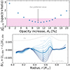 |
Fig. A.1. Optimized results of the K2-A2 models (see Table 2) with opacity increases (see Eqs. 2 and 3). Top: χ2 values with N = 6 as a function of the opacity increase parameter, A2. Bottom: Sound speed profile of models with A2 = 0, 3, 5, 8, 10, 12, 14, 16, 18, and 20% at the solar age, compared with helioseismic data in Basu et al. (2009), cs,obs. The model with our preferred value, A2 = 10%, is highlighted with the thick line. The dashed line illustrates the shape of the δκ function with an arbitrary +0.006 vertical shift. |
Figure A.2 shows that a higher A2 value leads to a stronger Li depletion in the pre-MS (from ∼3 to ∼20 Myr). This is because higher opacity at around the BCZ shifts RCZ downward and thus increases the temperature at the BCZ. Although this effect changes A(7Li) by up to ∼0.5 dex, the observational constraint of the present-day Sun, A(7Li)⊙ = 0.96 ± 0.05 dex, is even much lower than the extreme model with A2 = 20%, which leads to A(7Li) ∼ 2.2 dex.
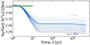 |
Fig. A.2. Evolution of the surface lithium abundance, A(7Li), of the K2-A2 models. The lines are color-coded by A2 as in the bottom panel of Fig. A.1. We note that the observational constraint of the present-day Sun, A(7Li)⊙ = 0.96 ± 0.05 dex, is not displayed in this plot. |
Appendix B: Models with diffusive overshooting
Here we show the K2-fov models that include diffusive overshooting, which can reproduce the solar Li abundance but are inconsistent with the observed trend of other solar-type stars. Diffusive overshooting corresponds to the model where the diffusion coefficient Dmix exponentially drops with the depth from the BCZ as (Herwig 2000)
 (B.1)
(B.1)
where D0 is the convective diffusion coefficient at the BCZ, Δr is the distance from the BCZ, HP is the pressure scale height at the BCZ, and fovershoot is a dimensionless parameter.
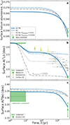 |
Fig. B.1. Same as Fig. 2 but showing the K2-fov models that include diffusive overshooting with fovershoot = 0.023 (dot-dashed gray line) and fovershoot = 0.01 (dotted). |
Figure B.1 shows the evolution of the surface He, Li, and Be abundances, as in Fig. 2. As described in Sect. 3, even the models without turbulent mixing or overshooting deplete Li in the pre-MS. Overshooting makes this Li burning more efficient by effectively deepening the surface CZ (see also Eggenberger et al. 2022; Buldgen et al. 2023). The model with fovershoot = 0.023 can reproduce A(7Li)⊙. However, in the MS, the Li burning is negligible, and thus A(7Li) is almost constant, unlike the observation of solar-type stars. Figure B.2 shows the Dmix profile. The Dmix of overshooting (Eq. B.1) rapidly drops just below the BCZ, whereas turbulent mixing exhibits a long tail down to ∼0.5 R⊙.
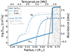 |
Fig. B.2. Profiles of Dmix (solid lines) of models K2-TM (blue) and K2-fov with fovershoot = 0.023 (gray) at the solar age. The dashed and dotted lines show the profiles of Li and Be abundances, respectively. The thin vertical dotted line shows the location of RCZ = 0.713 R⊙. |
In addition to the constant A(7Li) evolution in the MS, the shallow overshooting mixing has other problems: Figure B.1a shows that helium settling is not suppressed and thus the observed Ysurf is not reproduced. Overshooting does not reach the Be-burning region (∼3.5 MK) and thus A(9Be) is not sufficiently depleted (Fig. B.1c; the slight depletion after ∼1 Gyr is due to settling).
From the results above, we conclude that models with diffusive overshooting alone do not satisfy all the observed constraints simultaneously and suggest a deeper mixing in the radiative region.
Appendix C: Simulation results
In this appendix we provide the details of our simulation results. Tables C.1 and C.2 show the input parameters and results at 4.567 Gyr, respectively, which were optimized using the simplex method (Sect. 2).
Additional supplemental materials are available on Zenodo. These include a csv file summarizing the optimized input parameters and results of all the simulation models, and structure and evolution data of the optimized cases of models K2-MZvar-TM, K2-TM, K2-MZvar, and K2. In addition, animations of the evolutions of the optimized case of each model are also available on Zenodo. We used the input files of the MESA code provided in KG217, with modifications for turbulent mixing, AAG21 abundance scale, and opacity tables (see details in Appendix A).
Input parameters minimized using chi-squared simulations.
Results minimized by the chi-squared simulations.
The abundance of an element X is A(X)≡log(NX/NH) + 12, where NX is the number density. Throughout this paper, log ≡ log10.
We considered mixing only in the MS following previous studies (Proffitt & Michaud 1991; Buldgen et al. 2025a), but we confirmed that the choice of this starting time does not affect the conclusion of this study.
Elements are lumped into four groups and the diffusion velocity is calculated only for four representative elements, namely 1H, 4He, 16O, and 56Fe (see Sect. 5.4 of Paxton et al. 2011).
The opacity increase function in this study is a single Gaussian function and we did not consider other opacity increases (i.e., A1 = 0 and A3 = 0 in KG21).
The high Yproto value of noacc-noov was derived via extended calibration that includes Ysurf in target quantities (see Tables 1, A.1, and A.2 of KG21).
For optimization, N = 3 as described above, but here we also include Ysurf, RCZ, and rms(δcs) values to see the quality of the solutions.
All Tables
All Figures
|
Fig. 1. Schematic illustration showing the structure evolution (panel a; the so-called Kippenhahn diagram) and the Dmix profile at the solar age (panel b) of our fiducial model, K2-MZvar-TM (see Table 2). The convective zones are depicted as a cloudy region. The color of the shade in panel a shows Zaccretion. The two lines at the stellar surface and center illustrate metallicity by color. The two dashed green lines the locations at temperatures 2.5 × 10⁶ and 3.5 × 10⁶ K, indicative of Li and Be burning, respectively. |
| In the text | |
|
Fig. 2. Evolution of the surface abundances of helium (panel a), lithium (b), and beryllium (c). The red and blue lines show the models with variable and steady Zaccretion, respectively. The solid and dashed lines show the models with and without turbulent mixing, respectively. The dotted lines show the models from KGB22 (with AGSS09 abundances, without turbulent mixing but with overshooting). See Table 2 for more details. The green points show the observational constraints of the present-day Sun (see Table 1). The green shades show the meteoritic constraints (Lodders 2021) arbitrarily extending from 1 to 10 Myr. The crosses and small circles in panel b show the observed A(7Li) values of clusters (Dumont et al. 2021) and individual stars (Carlos et al. 2019), respectively, that are younger than the Sun. |
| In the text | |
|
Fig. 3. Solar metallicity profile at the present day of the six models shown in Fig. 2. The dashed vertical line shows the BCZ. See Fig. B.2 for the Dmix profile. |
| In the text | |
|
Fig. 4. Solar neutrino fluxes. The stars and circles show the models with variable and steady Zaccretion, respectively. Orange and brown illustrate the models with and without turbulent mixing, respectively. Blue shows the models from KGB22 (with AGSS09 abundances and without turbulent mixing). The points with error bars are the observational constraints (Table 1). The dotted cyan error bar shows an old constraint from Borexino Collaboration (2020). |
| In the text | |
|
Fig. 5. Evolution of Ysurf in model K2-MZvar-TM (solid red line) and a non-accreting model from KG21 with standard atomic diffusion (i.e., no overshooting and with turbulent mixing; dashed gray) starting with a high Yproto value within the range suggested by Serenelli & Basu (2010, blue shaded region). Turbulent mixing suppresses gravitational settling and thus leads to a reduced Yproto value. |
| In the text | |
|
Fig. A.1. Optimized results of the K2-A2 models (see Table 2) with opacity increases (see Eqs. 2 and 3). Top: χ2 values with N = 6 as a function of the opacity increase parameter, A2. Bottom: Sound speed profile of models with A2 = 0, 3, 5, 8, 10, 12, 14, 16, 18, and 20% at the solar age, compared with helioseismic data in Basu et al. (2009), cs,obs. The model with our preferred value, A2 = 10%, is highlighted with the thick line. The dashed line illustrates the shape of the δκ function with an arbitrary +0.006 vertical shift. |
| In the text | |
|
Fig. A.2. Evolution of the surface lithium abundance, A(7Li), of the K2-A2 models. The lines are color-coded by A2 as in the bottom panel of Fig. A.1. We note that the observational constraint of the present-day Sun, A(7Li)⊙ = 0.96 ± 0.05 dex, is not displayed in this plot. |
| In the text | |
|
Fig. B.1. Same as Fig. 2 but showing the K2-fov models that include diffusive overshooting with fovershoot = 0.023 (dot-dashed gray line) and fovershoot = 0.01 (dotted). |
| In the text | |
|
Fig. B.2. Profiles of Dmix (solid lines) of models K2-TM (blue) and K2-fov with fovershoot = 0.023 (gray) at the solar age. The dashed and dotted lines show the profiles of Li and Be abundances, respectively. The thin vertical dotted line shows the location of RCZ = 0.713 R⊙. |
| In the text | |
Current usage metrics show cumulative count of Article Views (full-text article views including HTML views, PDF and ePub downloads, according to the available data) and Abstracts Views on Vision4Press platform.
Data correspond to usage on the plateform after 2015. The current usage metrics is available 48-96 hours after online publication and is updated daily on week days.
Initial download of the metrics may take a while.