| Issue |
A&A
Volume 702, October 2025
|
|
|---|---|---|
| Article Number | A255 | |
| Number of page(s) | 8 | |
| Section | Extragalactic astronomy | |
| DOI | https://doi.org/10.1051/0004-6361/202555109 | |
| Published online | 24 October 2025 | |
Radiative signatures of electron-ion shocks in BL Lac type objects
1
Max-Planck-Institut für Physik, Boltzmannstr. 8, DE-85748 Garching, Germany
2
Max-Planck-Institut für Plasmaphysik, Boltzmannstr. 2, DE-85748 Garching, Germany
⋆ Corresponding authors: This email address is being protected from spambots. You need JavaScript enabled to view it.
; This email address is being protected from spambots. You need JavaScript enabled to view it.
; This email address is being protected from spambots. You need JavaScript enabled to view it.
Received:
10
April
2025
Accepted:
26
August
2025
Abstract
Aims. Plasma shock waves stand out as one of the most promising sites of efficient particle acceleration in extragalactic jets. In electron-ion plasma shocks, electrons can be heated up to large Lorentz factors, making them an attractive scenario to explain the high minimum electron Lorentz factors regularly needed to describe the emission of BL Lac type objects. Still, the (relativistic) thermal electron component is commonly neglected when modelling the observations, although it holds key information on the shock properties.
Methods. Considering a shock acceleration scenario, we modelled the broadband emission of the archetypal high synchrotron peaked blazar Markarian 421; we employed particle distributions that included a thermal (relativistic) Maxwellian component at low energies followed by a non-thermal power law, as motivated by particle-in-cell simulations. The observations, in particular in the optical/UV and MeV-GeV bands, efficiently restricted the non-thermal emission from the Maxwellian electrons, which we used to derive constraints on the basic properties, such as the fraction ϵe of the total shock energy stored in the non-thermal electrons.
Results. The best-fit model yields a non-thermal electron power law with an index of ∼2.4, close to predictions from shock acceleration. Successful fits are obtained when the ratio between the Lorentz factor at which the non-thermal distribution begins (γnth) and the dimensionless electron temperature (θ) satisfies γnth/θ ≲ 8. Since γnth/θ controls ϵe, the latter limit implies that at least ϵe ≈ 10% of the shock energy is transferred to the non-thermal electrons. These results are almost insensitive to the shock velocity γsh, but radio observations indicate γsh ≳ 5 since for lower shock velocities the fluxes in the millimetre band are overproduced by the Maxwellian electrons. Therefore, if shocks drive the particle energisation, our findings indicate that they operate in the mildly to fully relativistic regime with efficient electron acceleration. This paper lays the ground for future works, in which we will use plasma simulations to investigate if, and under which conditions, the findings presented here can be reproduced.
Key words: acceleration of particles / radiation mechanisms: non-thermal / shock waves / BL Lacertae objects: individual: Markarian 421 / galaxies: jets
© The Authors 2025
 Open Access article, published by EDP Sciences, under the terms of the Creative Commons Attribution License (https://creativecommons.org/licenses/by/4.0), which permits unrestricted use, distribution, and reproduction in any medium, provided the original work is properly cited.
This article is published in open access under the Subscribe to Open model.
Open access funding provided by Max Planck Society.
1. Introduction
Plasma shock waves are ubiquitous phenomena in galactic sources of high-energy radiation. They efficiently convert the kinetic energy of the plasma flow into the acceleration of particles up to relativistic speeds (e.g. Fermi 1949; Bell 1978; Drury 1983; Blandford & Eichler 1987). In extragalactic jets launched by active galactic nuclei (AGNs), mildly and/or fully relativistic shocks are also believed to play a central role in the energisation of charged particles up to ∼TeV energies (Blandford & Königl 1979; Marscher & Gear 1985; Kirk et al. 1998). Some of these regions may be associated with superluminal features observed at radio frequencies (e.g. Zensus 1997). Additional observational evidence was recently brought by the measurement of polarisation up to X-rays in the synchrotron spectrum of BL Lac type objects. Both in quiescent and flaring states, the X-ray polarisation angle aligns well on average with the angle measured at lower frequencies, as well as with the jet axis (e.g. Liodakis et al. 2022; MAGIC Collaboration 2025; Abe et al. 2024; Di Gesu et al. 2022). This behaviour is expected if a (self-generated) magnetic field component orthogonal to the jet axis develops at the shock front, as revealed by particle-in-cell (PIC) simulations (Crumley et al. 2019; Vanthieghem et al. 2020).
In the specific case of electron-ion plasma shocks, most of the available shock energy is contained in the ions. Part of the shock energy heats the electrons to a fraction of the equipartition, which leads to the development of thermal (relativistic) Maxwellian distribution that can easily peak at Lorentz factors of γ ∼ 102 − 103, even for mildly relativistic shocks. This motivates us to consider electron-ion shocks as a potential cause of the relatively high minimum electron Lorentz factors required to describe the spectral energy distribution (SED) of ‘extreme TeV’ BL Lac objects (Kaufmann et al. 2011; Costamante et al. 2018; Biteau et al. 2020; Zech & Lemoine 2021).
While PIC simulations of shocks indicate a thermal Maxwellian distribution in the low-energy part of the particle population, the modelling of the broadband emission from BL Lac objects (and blazars in general) is typically performed without considering this component (Böttcher et al. 2013; Tavecchio et al. 2010). The radiating particles are modelled with a power law, broken power law, or log-parabola distributions with a hard cutoff at low energies. However, even if located at the lowest energies, the non-thermal radiation signature of the Maxwellian component might in principle be detectable with gamma-ray instruments. Recently, Tavecchio et al. (2025) investigated the case of flat spectrum radio quasars (FSRQs), and show that a thermal particle population in electron-ion shocks may be constrained by MeV observatories.
Constraining the (relativistic) thermal distribution is highly relevant to extract fundamental properties of the shock, such as the fraction of shock and thermal energy that is conveyed to the non-thermal particles. Those properties can be subsequently tested with PIC simulations in order to further constrain shock parameters. Here, we study the case of BL Lac type objects, and in particular high synchrotron peaked (HSPs; Abdo et al. 2010) blazars. For HSPs, the non-thermal emission from the Maxwellian electrons in mildly and full relativistic electron-ion shocks is expected in the millimetre-to-infrared range as well as in the MeV-GeV gamma-ray band (assuming leptonic models; Mastichiadis & Kirk 1997; Krawczynski et al. 2004). Those energies, in particular the latter, are well covered by currently operating instruments. Exploiting a well-sampled SED from Abdo et al. (2011) of the HSP Markarian 421 (hereafter Mrk 421), we modelled the non-thermal emission with a PIC motivated electron distribution in order set limits on the basic properties of the Maxwellian distribution. This work is part of a broader effort; in our next step we plan to use dedicated PIC simulations to verify whether, and under which conditions of electron-ion shocks, the findings of this work can be matched.
The paper is structured as follows. Sections 2 and 3 describe the model and its application to Mrk 421. The results are shown in Sect. 4, and in Sect. 5 we discuss their implications for the shock parameters. Finally, the conclusions are drawn in Sect. 6.
2. Model setup
For simplicity and clarity, we considered an electron-proton plasma shock with an equal number density between the two particle species, η := ne/np = 1. Beyond the shock, the energetic particles are injected in the downstream region, where they emit non-thermal emission. As demonstrated by PIC simulations (e.g. Sironi & Spitkovsky 2011; Crumley et al. 2019), the low-energy part of the particle population is heated and forms a thermal component following a (relativistic) Maxwellian distribution. At higher energies, γ > γnth, a non-thermal power-law component develops as a result of first-order Fermi type shock acceleration. Such a distribution can be parametrised as described in Giannios & Spitkovsky (2009):
 (1)
(1)
where  describes the Maxwellian thermal component, θ ≡ kTe/mec2 is the dimensionless particle temperature, p1 is the power-law index of accelerated particles, and γnth designates the Lorentz factor at which the non-thermal particle distribution starts. The above parametrisation for the thermal component (𝒩(γ, θ)) is a generic functional form of a (relativistic) Maxwellian distribution valid in the limit where θ ≫ 1. As demonstrated in the following sections, this is expected even for mildly relativistic electron-ion shocks, and the fit results presented later further constrain θ ≫ 1. The adopted parametrisation is thus well justified.
In the downstream region, we calculated the resulting non-thermal radiation within the framework of a purely leptonic model using the same code as used in MAGIC Collaboration (2021). The broadband spectrum is ascribed to synchrotron self-Compton (SSC) emission, which is the simplest scenario that satisfactorily describes the SEDs of BL Lac, and HSPs in particular (see e.g. Mastichiadis & Kirk 1997; Tavecchio et al. 1998; Krawczynski et al. 2004). The code incorporates synchrotron self-absorption effects at radio frequencies using the equations in Appendix C of Zacharias (2015). We further assumed that particles escape the emitting region, approximated as a sphere, on timescales of tesc = R/c, where R is the radius of the region in the co-moving frame. The emission was calculated by assuming that the particle distribution reached its equilibrium state, taking into account particle escape and synchrotron radiation as the dominant cooling effect. In all the cases investigated in this work, synchrotron cooling becomes effective for electrons with a Lorentz factor γ ≳ 105, i.e., deep in the non-thermal part of the population. For γ ≲ 105, particles escape the downstream region before radiating a significant fraction of their energy. The equilibrium state of the particle distribution therefore has a spectral break of Δp = 1 in the power law where the electron cooling timescale equals the escape time, i.e. at  , where σT is the Thomson cross section and B the co-moving magnetic field (Kirk et al. 1998). Consequently, the electron distribution described by Eq. (1) was modified as follows:
 (2)
(2)
where γcut is the cutoff energy. If the electron temperature (θ) is sufficiently high, this distribution effectively mimics one with a high γmin (cf. Fig. 1). We employ this parametrisation for the SED modelling presented below.
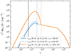 |
Fig. 1. Sample of electron distributions using Eq. (2) for different γnth/θ values ranging from 6 to 15. The dashed black line represents θ, which is fixed to 500. The coloured dotted lines give the location of γnth where the transition from the Maxwellian to the non-thermal component occurs. Here, we arbitrarily set γbr = 2 × 10⁵ and γcut = 7 × 10⁵ and p1 = 2.4. |
Two additional properties are conventionally used to characterise the particle distribution that results from an electron-proton shock: the fraction Δ of the total electron energy residing in the non-thermal component, and the fraction ϵe of the total shock energy carried by the non-thermal electrons. We defined Δ as in Giannios & Spitkovsky (2009):
 (3)
(3)
while ϵe is given by
 (4)
(4)
where np is the proton number density and γ0 is the bulk Lorentz factor of the upstream plasma (jet plasma before the shock) as observed in the downstream frame (the emitting region). Several factors detetermin γ0, such as θ and the temperature ratio between the protons and electrons, which we assumed to be Te/Tp = 0.5 for the rest of this work (this is compatible with PIC simulations of relativistic electron-ion shocks, see Sironi & Spitkovsky 2011). The corresponding functional form of γ0 is derived in Sect. 5. Following Tavecchio et al. (2025), the above expression can be simplified by introducing  , the average electron Lorentz factor, and η:
 (5)
(5)
As already mentioned, in what follows we used η = 1.
It is important to note that the ratio γnth/θ directly dictates Δ, and therefore also ϵe. A higher γnth/θ value leads to a more prominent Maxwellian component with respect to the non-thermal part, at the cost of reducing Δ and ϵe. Figure 1 shows the electron distribution using Eq. (2) for several γnth/θ values from 6 to 15. The corresponding values of Δ and ϵe are given in the legend.
3. Application to the TeV BL Lac object Mrk 421
We applied our model to the archetypal TeV BL Lac object Mrk 421 (z = 0.031). Due to its brightness and proximity, Mrk 421 is one of the blazars whose broadband SED shape can be determined with exceptional precision even when the source shows very low activity (for recent multi-wavelength campaigns, see e.g. Baloković et al. 2016; MAGIC Collaboration 2021; Abe et al. 2024). Using a precise broadband SED of Mrk 421, we intend to constrain the contribution of a Maxwellian component to set limits on the shock parameters, focusing on Δ and ϵe.
In the case of mildly relativistic shocks with γsh ∼ (2 − 5), equivalent to θ ∼ (102 − 5 × 10²) (see Sect. 5 and Eqs. (11) and (12)), the maximum of the Maxwellian distribution is located at  . If we associate this peak with an effective minimum Lorentz factor, high values of γmin ∼ 103 could be accommodated. The synchrotron emission of the thermal electrons is then expected to peak at a (observed) frequency of
 (6)
(6)
where δ is the Doppler factor of the emitting region. Considering typical values of the magnetic field and Doppler factor inferred from blazar SED modelling (B ∼ 0.1 G and δ ∼ 20; Tavecchio et al. 2010; Abdo et al. 2011), νsyn ∼ 1011 − 1014 Hz, i.e. in the millimetre to infrared band. As for their inverse-Compton contribution, the emitted frequency in one-zone SSC models is approximately (assuming the Thomson regime, as is typically the case for Lorentz factors of  )
)
 (7)
(7)
where νsyn, peak is the peak frequency of the synchrotron component in the SED (Tavecchio et al. 1998). In the specific case of the HSP Mrk 421, this SED peak frequency, νsyn, peak, is around 1017 Hz, which implies a possible contribution of the Maxwellian component from ∼10 MeV to ∼10 GeV depending on the exact value of θ (and thus  ). The MeV-GeV band is ideally covered by gamma-ray observatories such as Fermi-LAT (Atwood et al. 2009; Ackermann et al. 2012), thus providing the opportunity to constrain the contribution of the Maxwellian hump. In passing, we note that since the radiative signature of Maxwellian electrons is expected at the rising edges of the two SED components, the hints of narrow features at the falling edges of the two SED components that were reported in the X-ray spectrum of Mrk 421 (presented in Acciari et al. 2021) and the TeV spectrum of the HSP Mrk 501 (presented in MAGIC Collaboration 2020) must have a different origin.
We used the broadband SED of Mrk 421 obtained during an average emission state published in Abdo et al. (2011). The SED was averaged over a six-month period in 2009 during which moderate variability had been detected; this suggests the absence of significant change in the source properties and particle distribution. Hence, to model the particle distribution, it seems appropriate to employ a steady-state solution following Eq. (2), which may result from an injection of particles at a constant rate in an emitting region whose physical properties stay roughly constant.
We started by determining the parameters related to the source environment δ, R, and B, as well as those of the electron distribution that can be derived independently of the Maxwellian component, that is, p1 and γcut. The peak luminosities and frequencies (that are unaffected by the Maxwellian component, unless in the most extreme cases) constrain δ, R, and B when considering a one-zone SSC model (Tavecchio et al. 1998). The p1 and γcut parameters are constrained by the optical-to-X-ray part of the SED, in which the Maxwellian contribution is also negligible. The break Lorentz factor γbr is not a free parameter of the system and is given by the synchrotron cooling break (i.e. it is a function of R and B). Prior to this initial fit, we set θ = γnth such that the Maxwellian component is suppressed, and arbitrarily assumed θ = 103, which satisfactorily describes the optical and MeV-GeV data without overproducing the radio fluxes. The SED was fitted by performing a scan over δ (from 10 to 30), and letting all other parameters free at each step. We then selected the set of parameters with the lowest χ2 and for which R < δ c tvar, where tvar is the source variability timescale, which is ≈1 day (Abdo et al. 2011). The resulting set of parameters is given in Table 1. The inferred γcut is in principle compatible with expectations of first-order Fermi acceleration at internal shocks (e.g. Rieger et al. 2007). The values reported here are very similar to those found by Nigro et al. (2022) after applying different fitting procedures to the same SED of Mrk 421.
SSC model parameters fixed throughout the work.
In a second step, we studied the effect of the thermal component on the observed SED by scanning multiple θ and γnth values while fixing the other parameters to those of Table 1 and keeping the synchrotron peak luminosity to a constant level by only modifying the electron density. Figure 2 shows test cases for different γnth/θ ratios, and θ = 100 (left panel) and θ = 500 (right panel). Such θ values correspond to a shock velocity (in the upstream frame) of γsh = 1.8 and γsh = 5.3, respectively, assuming a temperature ratio of Te/Tp = 0.5 between the electrons and protons. We refer the reader to Sect. 5 for more details on the relation between θ and γsh.
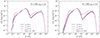 |
Fig. 2. SED models for θ = 100 (left) and θ = 500 (right), corresponding to a shock velocity (in the upstream frame) of γsh = 1.8 and γsh = 5.3, respectively. We refer the reader to Sect. 5 for more details on the connection between θ and γsh. Solid lines, from light violet to dark violet, cover three different γnth/θ ratios, 4, 7, and 10. The SED from Abdo et al. (2011) is plotted with grey markers. |
The model starts to exceed the MeV-GeV part of the observed SED (covered by Fermi-LAT) for γnth/θ > 7. The model also exceeds the optical data around 10−1 eV for θ = 500 and γnth/θ > 7. These spectral features allow us to set limits on γnth/θ, which controls the amount of energy transferred from the shock to the non-thermal electrons, hence constraining ϵe and Δ. The prominence of the Maxwellian signature and its broad radiative pattern enable us to set limits on γnth/θ that are to a large extent independent from the exact value of the parameters such as δ, R, and B (i.e. the parameters with the highest degree of degeneracy in one-zone models).
We systematically explored the range of γnth/θ allowed by the data by repeating the same procedure as for Fig. 2. We scanned a wider range of θ and γnth/θ ratios, and computed at each step the χ2 as a measure of the disagreement between the model and the data. The χ2 is calculated above the radio band, i.e., beyond 10−1 eV since due to synchrotron self-absorption it is known that one-zone SSC models fail to reproduce the radio spectra of blazars. The unsuitability of one-zone SSC models to simultaneously describe the very-high-energy (E > 100 GeV) and radio spectra is thus independent of the used electron distribution. Hence, it is not meaningful to use a χ2 test to quantify the disagreement between the model and the data in an energy range that is known to be poorly reproduced by the model. Additionally, the radio band likely receives a significant contribution from large-scale structures in the jet that are broader and likely farther downstream than the compact region modelled here. In what follows, we therefore consider the radio observations as upper limits to constrain the value of θ from below. The χ2 is calculated assuming a conservative 15% systematic uncertainty on the fluxes for all measurements.
4. Results
Figure 3 shows Δχ2 = χ2 − χmin2 as a function of γnth/θ, where χmin2 is the minimum value for a given θ. The scans were performed for θ = [100, 300, 500, 1500], corresponding to a shock velocity of γsh = [1.8, 3.5, 5.3, 13.9] (for Te/Tp = 0.5; see Sect. 5), representative of mildly to fully relativistic shocks (see below). The χ2 values increase significantly for high γnth/θ ≳ 7 − 8 due to an overestimation of the optical/UV and MeV-GeV fluxes when the thermal component becomes dominant. For θ = 1500, χ2 also increases in the range γnth/θ ∼ 2 − 6. With such a large θ, electrons emit photons primarily in the MeV-GeV band, and increasing γnth results in an underproduction of the Fermi-LAT spectrum by the non-thermal electrons. For γnth/θ ≳ 6, the Maxwellian component becomes significant enough to compensate for this deficit. We emphasize that this deficit in the model could potentially be explained by invoking additional, unconstrained emitting regions in the jet. Consequently, Fig. 3 only allows us to constrain the upper limit of γnth/θ.
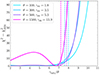 |
Fig. 3. The difference χ2 − χmin2 as a function of γnth/θ, for θ = [100, 300, 500, 1500], equivalent to a shock velocity of γsh = [1.8, 3.5, 5.3, 13.9]. We refer the reader to Sect. 5 for more details on the connection between θ and γsh. We denote by χmin2 the minimum χ2 for a given θ. The vertical dashed lines mark the γnth/θ value beyond which χ2 − χmin2 > 9. |
The χ2 values degrade beyond γnth/θ ≳ 7 − 8, irrespective of the value of θ. Vertical dashed lines in Fig. 3 indicate, for each θ, where χ2 − χmin2 > 9. We have chosen this threshold arbitrarily to roughly identify the range of γnth/θ values that are inconsistent with the data, as this value is commonly used to set upper limits at the 3σ confidence level in χ2 tests. We emphasize that a precise determination of the upper limits on γnth/θ requires a more rigorous statistical analysis, including a proper consideration of the instrument response functions and instrumental systematics. This is beyond the scope of this work. In Appendix A, we present the SED for each θ and with γnth/θ in the transition region where the fits degrade, i.e., from γnth/θ = 6 to γnth/θ = 10. These SEDs clearly illustrate that, regardless of a detailed statistical treatment, γnth/θ ≳ 8 is inconsistent with the data.
The model overproduces the radio emission at energies from E ∼ 10−5 eV to E ∼ 10−3 eV for θ < 500. For θ ≳ 500, the model only exceeds the radio fluxes when γnth/θ ≳ 8, but these values are already excluded by our parameter scan (see Fig. 3). Consequently, our investigations simultaneously constrain γnth/θ ≲ 8 and θ ≳ 500. Considering these constraints, and using the parameters in Table 1, our one-zone model achieves the best description of the optical-to-TeV data for θ ≈ 500 and γnth/θ ≈ 6. The corresponding electron distribution is plotted with the darkest blue line in Fig. 1.
To remain compatible with the upper limits from radio data even with θ ≲ 500, one may try to determine a parameter set that provides an emitting region that is significantly more compact. In this case, the synchrotron self-absorption frequency may reach up to the millimetre range. However, as discussed in Tavecchio et al. (1998), the one-zone SSC model is a closed system. Once constraints from variability timescales and the (synchrotron) cooling break are included, there is very little freedom in choosing the parameter values. The observable νsyn, peak sets γbr, which is in turn dictated by the size of the emitting region and the magnetic field as a consequence of synchrotron cooling. Therefore, within our single-zone scenario, an agreement with the radio data for θ ≲ 500 is not possible. The only alternative is to make ad hoc assumptions on the shape of the electron distribution to include additional spectral breaks and/or to fully decouple γbr, B, and R to allow a synchrotron self-absorption frequency in the millimetre range. In principle, one could also consider the possibility of a spectral break deviating from the standard cooling break of 1, perhaps due to inhomogeneities within the emitting region. These considerations, which have been discussed elsewhere (e.g. Abdo et al. 2011; Baheeja et al. 2022), are beyond the scope of the current study.
Figure 4 gives the evolution of Δ and ϵe as a function of γnth/θ. The region constrained by the SED of Mrk 421 lies left from the vertical dashed black line placed at γnth/θ = 8, being roughly the maximum value that we found compatible with the measurements. The two quantities show little dependency on θ. Therefore, independently of the choice of θ, we infer that the particle distribution must be characterised by Δ ≳ 0.4 and ϵe ≳ 10−1 in order to be in agreement with the data.
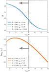 |
Fig. 4. The top and bottom panels shows Δ and ϵe (using Eq. (3) and Eq. (4)) versus γnth/θ, respectively. The allowed region lies to the left of the vertical dashed black line placed at γnth/θ = 8, which is roughly the maximum value that we found compatible with the measurements. |
To verify the energy requirements, we estimate the kinetic jet power as
 (8)
(8)
where Γb ≈ δ is the bulk Lorentz factor of the emitting region in the observer’s frame,  the electron energy density, uB = B2/8π the magnetic energy density, and up ≈ np mpc2 is the (cold) proton energy density. We assume an equal number density of protons and electrons, such that np = ne. For all cases satisfying γnth/θ ≲ 8, we find Ljet, kin ≲ 1045 erg s−1. This is well below the Eddington luminosity LEdd ≈ 3 × 1046 erg s−1 for the estimated black hole mass of Mrk 421 (MBH ≃ 2 × 10⁸ M⊙; Barth et al. 2003). As expected, Ljet, kin decreases with increasing θ because the electron density is dominated by particles at the lowest energies. For our best-fit case (θ ≈ 500 & γnth/θ ≈ 6), the kinetic jet power is Ljet, kin ≈ 5 × 1043 erg s−1.
5. Relationship to shock parameters
As demonstrated above, in principle SED modelling allows us to place constraints on the shape of the thermal component. These constraints can, in turn, inform plasma simulations of mildly relativistic shocks. Conversely, simulations of shock physics can provide insight into the suitability of a given SED model. However, this requires relating the inferred parameters to those commonly employed in simulations, which we address in the following.
We use γ0 to denote the bulk Lorentz factor of the upstream plasma as measured in the downstream reference frame. At the shock, the incoming kinetic energy of the plasma is redistributed among thermal and non-thermal protons and electrons. For shocks that are accompanied by efficient particle acceleration, only a fraction ath < 1 of the upstream energy is transferred to thermal protons and electrons, i.e., we have
 (9)
(9)
where γth, e and γth, p are the average thermal electron and ion Lorentz factor at the shock downstream, respectively, and where we take ath ≈ 0.8 as the fiducial reference value. Protons and electron are usually not in thermal equilibrium with each other downstream of the shock (Raymond et al. 2023), so that
 (10)
(10)
In PIC simulations of quasi-parallel, mildly relativistic (γsh ≃ 2), and weakly magnetised electron-ion shocks, for example, Te ∼ 0.25 Tp has been observed (Crumley et al. 2019). Electron heating might be further enhanced for weakly magnetised (Te ∼ 0.3 Tp, Vanthieghem et al. 2020) or more relativistic shocks (Te ∼ 0.5 Tp, Sironi & Spitkovsky 2011; Sironi et al. 2013).
Taking into account Eq. (9), Eq. (10), and  , the relationship between γ0 and θ can be expressed as
 (11)
(11)
The Lorentz factor of the shock γsh and γ0 are approximately related by (Nishikawa et al. 2009)
 (12)
(12)
where Γad = 4/3 is the adiabatic index of three-dimensional relativistic gas. Taking the best-fit case assuming a one-zone model, θ ≈ 500 (see Sect. 4), which yields γsh ≈ 5.3 (assuming ath = 0.8 and Te/Tp = 0.5). A key parameter in shock simulations is the magnetisation of the upstream plasma:
 (13)
(13)
where B0 is the upstream magnetic field and n0 is the upstream plasma density measured in the downstream reference frame. SED modelling constrains the magnetic field, B, and particle density, n, of the downstream plasma measured in the co-moving (downstream) reference frame. The upstream plasma density can be estimated using the shock compression ratio  (Nishikawa et al. 2009). Accordingly, the upstream plasma density becomes
 (14)
(14)
The relationship between the magnetic field in the upstream and downstream regions of the shock is not straightforward. It depends on several factors, including magnetic field amplification in the foreshock region, compression at the shock, and decay in the downstream region. These processes, in turn, are influenced by the shock Lorentz factor, magnetisation, and obliquity. PIC simulations (e.g. Sironi & Spitkovsky 2011; Sironi et al. 2013; Crumley et al. 2019) indicate that approximately 10% of the upstream kinetic energy in mildly relativistic shocks is converted into magnetic energy at the shock transition. However, these simulations also show that the self-generated magnetic field decays rapidly in the downstream region, on scales of about a thousand of ion skin depths, 1000λsi ∼ 109 cm, which is much smaller than the size of the emitting region, R ∼ 1016 cm. Since PIC simulations only probe turbulence on microscopic scales, it seems possible that turbulence driven on larger scales may decay more slowly (e.g. Lemoine 2013), potentially influencing the entire emission region. Indeed, in the case of unmagnetised shocks (Chang et al. 2008) mediated by the Weibel instability (Weibel 1959), turbulence on larger scales decays much more slowly. However, this topic remains largely unexplored, which makes a robust quantitative extrapolation to macroscopic scales difficult. In view of this, we assume the upstream magnetic field to be B0 = B/aB, where aB represents the cumulative magnetic field amplification. In the case of very weak magnetic field amplification or fast field decay, aB = 1 corresponds to a parallel shock, while aB = γ0r corresponds to a perpendicular shock.
By combining the expressions for the plasma density and the magnetic field with Eq. (13), the upstream plasma magnetisation can be expressed as
![Mathematical equation: $$ \begin{aligned} \sigma =\frac{(B/a_\mathrm{B} )^2}{4 \pi \gamma _\mathrm{0} n (m_{\rm p}+m_\mathrm{e} ) c^2} \frac{\Gamma _\mathrm{ad} (\gamma _\mathrm{0} +1)}{[\gamma _\mathrm{0} (\Gamma _\mathrm{ad} -1)]}\cdot \end{aligned} $$](/articles/aa/full_html/2025/10/aa55109-25/aa55109-25-eq24.gif) (15)
(15)
In the case under consideration, with θ = 500, the electron density in the emitting region is n ∼ 1 cm−3 and the upstream plasma magnetisation is constrained to σ ∼ 0.15/aB2.
6. Conclusions
Particle-in-cell simulations of plasma shocks demonstrate the development of a thermal component in the low-energy part of the distribution (e.g. Sironi & Spitkovsky 2011; Crumley et al. 2019). For electron-ion shocks, the electron thermal component can easily peak at Lorentz factors as high as γ ∼ 102 − 103, effectively mimicking an electron distribution with high γmin. In this work, we have modelled the broadband emission of the BL Lac type object Mrk 421 by adopting an electron distribution composed of a (relativistic) thermal Maxwell distribution and a non-thermal (broken) power-law component. While we cannot claim the existence of a thermal (Maxwellian) population from observations (from radio frequencies to TeV), such a component is expected from first principles. In this work, we show that the broadband data greatly restrict the contribution of the Maxwellian electrons, providing constraints on the physical properties of the shock.
To avoid overproducing the observed fluxes in the optical/UV and MeV-GeV bands (where the thermal electrons emit most of their radiation), we find that the ratio between the Lorentz factor at which the non-thermal distribution begins (γnth) and the dimensionless electron temperature (θ) must satisfy γnth/θ ≲ 8. Since γnth/θ controls the fraction Δ of the total electron energy residing in the non-thermal component, and the fraction ϵe of the total shock energy carried by the non-thermal electrons, the limit γnth/θ ≲ 8 translates into the following constraints: Δ ≳ 0.4 and ϵe ≳ 10−1. Such a limit for ϵe seems broadly consistent with simulations of relativistic shock (e.g. Sironi & Spitkovsky 2011). Dedicated PIC simulations are needed to verify the extent to which these results can be reproduced under the inferred conditions, a task we intend to address in a subsequent study. It is important to note that the constraints we obtain are only slightly dependent on the value of θ, and thus on the shock velocity (see Sect. 5). However, to stay below the radio fluxes, θ ≳ 500, which suggests that γsh ≳ 5.3 assuming ath = 0.8 and Te/Tp = 0.5 and using Eq. (12). Our analysis therefore favours shocks in the mildly or fully relativistic regime.
Broadband modelling of HSPs, ‘extreme TeV’ blazars, and recent X-ray polarisation results suggest a relatively high γmin, up to ∼104 (see e.g. Costamante et al. 2018; MAGIC Collaboration 2025). While the Maxwellian component is often neglected in the literature, if one were to equate γmin with γnth, then γmin ∼ 104 would imply θ ∼ 1000 and γnth/θ ∼ 8, a scenario that is still consistent with our parameter scan. Alternatively, as discussed in Zech & Lemoine (2021), a sequence of multiple shocks could elevate an initial (lower) value of γmin, potentially leading to the values considered here.
The model employed here considers a single emission zone, whereas multiple regions within the jet may contribute to the overall SED. This limitation explains why we can only establish upper limits on γnth/θ, and consequently, our conclusions remain largely unaffected by the potential contribution of multiple emission zones. However, the interaction of electrons with the radiation field from other jet regions (as in the ‘spine-layer’ model; Ghisellini et al. 2005) could alter the inverse-Compton spectral shape compared to that predicted by the single-zone model. This alteration may influence our limits, as they are directly dependent on the radiative signatures observed in the gamma-ray band. A detailed study is necessary to accurately evaluate this impact. Nevertheless, we anticipate that achieving a satisfactory description of the gamma-ray data for γnth/θ > 8 would necessitate a significant (and unnatural) fine-tuning of the external photon field spectrum, given the distinct (and broad) signature of the Maxwellian electrons (see Appendix A).
Under the assumption that a single zone is responsible for the emission from optical to TeV, our best fit is obtained for γnth/θ ≈ 6 and θ ≈ 500, i.e., γsh ≈ 5.3 (again for ath = 0.8 and Te/Tp = 0.5). This could be compared to simulations of subluminal mildly relativistic shocks where strong electron heating and efficient particle acceleration with ϵe ≈ 0.1 has been observed (Sironi & Spitkovsky 2011). In the framework of a ‘blob-in-jet’ scenario, where a fast (Γb) obstacle overtakes the jet (Γj < Γb), γsh ≃ Γb/2Γj (e.g. Zech & Lemoine 2021). For a closely aligned jet, where δ ∼ Γb, the inferred mean jet flow speeds would then be on the order of Γj ∼ Γb/2γsh∼ a few. Considering a stationary shock, the jet Lorentz factor must obey Γj ≳ γshδ/2 ∼ 50. Such a value is at the extreme of the distribution of Lorentz factors obtained from very-long-baseline interferometry (VLBI) observations of parsec-scale jets (Homan et al. 2021).
The temperature ratio Te/Tp = 0.5 assumed throughout this work is compatible with PIC simulations of relativistic electron-ion shocks, as reported in Sironi & Spitkovsky (2011). Similar values are found by Crumley et al. (2019) for the mildly relativistic case. We note that the temperature ratio is sensitive to other parameters such as magnetisation. Nevertheless, the results reported in the works mentioned above cover a range of magnetisation (and γsh) that is comparable to the one derived using our phenomenological model. Therefore, assuming Te/Tp = 0.5 is a well-motivated initial guess, and also our conclusions do not strongly depend on the exact value of Te/Tp. To obtain a more accurate determination of the temperature ratio, one would need to explore a wide range of γ0 and magnetisation with PIC simulations, which we leave for a future work.
Our model was applied to the average emission state of Mrk 421 observed in 2009, a period characterised by an extended phase of low flux variability (Abdo et al. 2011). Rapid outbursts, frequently observed in blazars and, by definition, representing peculiar source states, are potentially caused by shocks with distinct physical conditions compared to those associated with the quasi-stable, quiescent emission. Further investigation into the connection between shock dynamics and emission statesis crucial for a complete understanding of the mechanisms that drive rapid outbursts. We defer the investigation of flaring events to future work.
The results presented here contribute to the development of a comprehensive model for understanding shock acceleration in blazar jets. High-quality SED characterisations, such as the ones that can be achieved with long multi-instrument observations of bright blazars, combined with dedicated simulations, will play a key role in further advancements in this model.
Acknowledgments
We thank Lea Heckmann for fruitful discussions in the early phases of the project, as well as Martin Lemoine for useful exchanges. We also acknowledge support from the Deutsche Forschungs gemeinschaft (DFG, German Research Foundation) under Germany’s Excellence Strategy – EXC-2094 –390783311.
References
- Abdo, A. A., Ackermann, M., Agudo, I., et al. 2010, ApJ, 716, 30 [NASA ADS] [CrossRef] [Google Scholar]
- Abdo, A. A., Ackermann, M., Ajello, M., et al. 2011, ApJ, 736, 131 [Google Scholar]
- Abe, S., Abhir, J., Acciari, V. A., et al. 2024, A&A, 684, A127 [NASA ADS] [CrossRef] [EDP Sciences] [Google Scholar]
- Acciari, V. A., Ansoldi, S., Antonelli, L. A., et al. 2021, MNRAS, 504, 1427 [Google Scholar]
- Ackermann, M., Ajello, M., Albert, A., et al. 2012, ApJS, 203, 4 [Google Scholar]
- Atwood, W. B., Abdo, A. A., Ackermann, M., et al. 2009, ApJ, 697, 1071 [CrossRef] [Google Scholar]
- Baheeja, C., Sahayanathan, S., Rieger, F. M., Jagan, S. K., & Ravikumar, C. D. 2022, MNRAS, 514, 3074 [Google Scholar]
- Baloković, M., Paneque, D., Madejski, G., et al. 2016, ApJ, 819, 156 [Google Scholar]
- Barth, A. J., Ho, L. C., & Sargent, W. L. W. 2003, ApJ, 583, 134 [NASA ADS] [CrossRef] [Google Scholar]
- Bell, A. R. 1978, MNRAS, 182, 147 [Google Scholar]
- Biteau, J., Prandini, E., Costamante, L., et al. 2020, Nat. Astron., 4, 124 [Google Scholar]
- Blandford, R., & Eichler, D. 1987, Phys. Rep., 154, 1 [Google Scholar]
- Blandford, R. D., & Königl, A. 1979, ApJ, 232, 34 [Google Scholar]
- Böttcher, M., Reimer, A., Sweeney, K., & Prakash, A. 2013, ApJ, 768, 54 [Google Scholar]
- Chang, P., Spitkovsky, A., & Arons, J. 2008, ApJ, 674, 378 [NASA ADS] [CrossRef] [Google Scholar]
- Costamante, L., Bonnoli, G., Tavecchio, F., et al. 2018, MNRAS, 477, 4257 [NASA ADS] [CrossRef] [Google Scholar]
- Crumley, P., Caprioli, D., Markoff, S., & Spitkovsky, A. 2019, MNRAS, 485, 5105 [NASA ADS] [CrossRef] [Google Scholar]
- Di Gesu, L., Tavecchio, F., Donnarumma, I., et al. 2022, A&A, 662, A83 [NASA ADS] [CrossRef] [EDP Sciences] [Google Scholar]
- Drury, L. O. 1983, Rep. Progr. Phys., 46, 973 [Google Scholar]
- Fermi, E. 1949, Phys. Rev., 75, 1169 [NASA ADS] [CrossRef] [Google Scholar]
- Ghisellini, G., Tavecchio, F., & Chiaberge, M. 2005, A&A, 432, 401 [CrossRef] [EDP Sciences] [Google Scholar]
- Giannios, D., & Spitkovsky, A. 2009, MNRAS, 400, 330 [NASA ADS] [CrossRef] [Google Scholar]
- Homan, D. C., Cohen, M. H., Hovatta, T., et al. 2021, ApJ, 923, 67 [NASA ADS] [CrossRef] [Google Scholar]
- Kaufmann, S., Wagner, S. J., Tibolla, O., & Hauser, M. 2011, A&A, 534, A130 [NASA ADS] [CrossRef] [EDP Sciences] [Google Scholar]
- Kirk, J. G., Rieger, F. M., & Mastichiadis, A. 1998, A&A, 333, 452 [NASA ADS] [Google Scholar]
- Krawczynski, H., Hughes, S. B., Horan, D., et al. 2004, ApJ, 601, 151 [NASA ADS] [CrossRef] [Google Scholar]
- Lemoine, M. 2013, MNRAS, 428, 845 [NASA ADS] [CrossRef] [Google Scholar]
- Liodakis, I., Marscher, A. P., Agudo, I., et al. 2022, Nature, 611, 677 [CrossRef] [Google Scholar]
- MAGIC Collaboration (Acciari, V. A., et al.) 2020, A&A, 637, A86 [NASA ADS] [CrossRef] [EDP Sciences] [Google Scholar]
- MAGIC Collaboration (Acciari, V. A., et al.) 2021, A&A, 655, A89 [NASA ADS] [CrossRef] [EDP Sciences] [Google Scholar]
- MAGIC Collaboration (Abe, K., et al.) 2025, A&A, 695, A217 [Google Scholar]
- Marscher, A. P., & Gear, W. K. 1985, ApJ, 298, 114 [Google Scholar]
- Mastichiadis, A., & Kirk, J. G. 1997, A&A, 320, 19 [NASA ADS] [Google Scholar]
- Nigro, C., Sitarek, J., Gliwny, P., et al. 2022, A&A, 660, A18 [NASA ADS] [CrossRef] [EDP Sciences] [Google Scholar]
- Nishikawa, K. I., Niemiec, J., Hardee, P. E., et al. 2009, ApJ, 698, L10 [Google Scholar]
- Raymond, J. C., Ghavamian, P., Bohdan, A., et al. 2023, ApJ, 949, 50 [NASA ADS] [CrossRef] [Google Scholar]
- Rieger, F. M., Bosch-Ramon, V., & Duffy, P. 2007, Ap&SS, 309, 119 [NASA ADS] [CrossRef] [Google Scholar]
- Sironi, L., & Spitkovsky, A. 2011, ApJ, 726, 75 [NASA ADS] [CrossRef] [Google Scholar]
- Sironi, L., Spitkovsky, A., & Arons, J. 2013, ApJ, 771, 54 [Google Scholar]
- Tavecchio, F., Maraschi, L., & Ghisellini, G. 1998, ApJ, 509, 608 [Google Scholar]
- Tavecchio, F., Ghisellini, G., Ghirlanda, G., Foschini, L., & Maraschi, L. 2010, MNRAS, 401, 1570 [Google Scholar]
- Tavecchio, F., Nava, L., Sciaccaluga, A., & Coppi, P. 2025, A&A, 694, L3 [NASA ADS] [CrossRef] [EDP Sciences] [Google Scholar]
- Vanthieghem, A., Lemoine, M., Plotnikov, I., et al. 2020, Galaxies, 8, 33 [NASA ADS] [CrossRef] [Google Scholar]
- Weibel, E. S. 1959, Phys. Rev. Lett., 2, 83 [NASA ADS] [CrossRef] [Google Scholar]
- Zacharias, M. 2015, MNRAS, 447, 2021 [Google Scholar]
- Zech, A., & Lemoine, M. 2021, A&A, 654, A96 [NASA ADS] [CrossRef] [EDP Sciences] [Google Scholar]
- Zensus, J. A. 1997, ARA&A, 35, 607 [NASA ADS] [CrossRef] [Google Scholar]
Appendix A: SED scans
Figure A.1 presents the SED model for all values of θ considered in this study, θ = [100, 300, 500, 1500]. The model is shown for a few values of γnth/θ around the transition region where the fit significantly degrades.
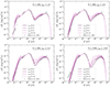 |
Fig. A.1. SED models for θ = [100, 300, 500, 1500]. Solid lines, from light violet to dark violet, cover three different γnth/θ = [6, 8, 9, 9], i.e. the transition region where the fit degrades. For each θ, the corresponding shock velocity γsh is also given. We refer the reader to Sect. 5 for more details on the connection between θ and γsh. The SED from Abdo et al. (2011) is plotted with grey markers. |
All Tables
All Figures
|
Fig. 1. Sample of electron distributions using Eq. (2) for different γnth/θ values ranging from 6 to 15. The dashed black line represents θ, which is fixed to 500. The coloured dotted lines give the location of γnth where the transition from the Maxwellian to the non-thermal component occurs. Here, we arbitrarily set γbr = 2 × 10⁵ and γcut = 7 × 10⁵ and p1 = 2.4. |
| In the text | |
|
Fig. 2. SED models for θ = 100 (left) and θ = 500 (right), corresponding to a shock velocity (in the upstream frame) of γsh = 1.8 and γsh = 5.3, respectively. We refer the reader to Sect. 5 for more details on the connection between θ and γsh. Solid lines, from light violet to dark violet, cover three different γnth/θ ratios, 4, 7, and 10. The SED from Abdo et al. (2011) is plotted with grey markers. |
| In the text | |
|
Fig. 3. The difference χ2 − χmin2 as a function of γnth/θ, for θ = [100, 300, 500, 1500], equivalent to a shock velocity of γsh = [1.8, 3.5, 5.3, 13.9]. We refer the reader to Sect. 5 for more details on the connection between θ and γsh. We denote by χmin2 the minimum χ2 for a given θ. The vertical dashed lines mark the γnth/θ value beyond which χ2 − χmin2 > 9. |
| In the text | |
|
Fig. 4. The top and bottom panels shows Δ and ϵe (using Eq. (3) and Eq. (4)) versus γnth/θ, respectively. The allowed region lies to the left of the vertical dashed black line placed at γnth/θ = 8, which is roughly the maximum value that we found compatible with the measurements. |
| In the text | |
|
Fig. A.1. SED models for θ = [100, 300, 500, 1500]. Solid lines, from light violet to dark violet, cover three different γnth/θ = [6, 8, 9, 9], i.e. the transition region where the fit degrades. For each θ, the corresponding shock velocity γsh is also given. We refer the reader to Sect. 5 for more details on the connection between θ and γsh. The SED from Abdo et al. (2011) is plotted with grey markers. |
| In the text | |
Current usage metrics show cumulative count of Article Views (full-text article views including HTML views, PDF and ePub downloads, according to the available data) and Abstracts Views on Vision4Press platform.
Data correspond to usage on the plateform after 2015. The current usage metrics is available 48-96 hours after online publication and is updated daily on week days.
Initial download of the metrics may take a while.