| Issue |
A&A
Volume 702, October 2025
|
|
|---|---|---|
| Article Number | A67 | |
| Number of page(s) | 14 | |
| Section | Extragalactic astronomy | |
| DOI | https://doi.org/10.1051/0004-6361/202555117 | |
| Published online | 10 October 2025 | |
Optical emission line properties of eROSITA-selected SDSS-V galaxies
1
Max-Planck-Institute for Astronomy, Königstuhl 17, D-69117 Heidelberg, Germany
2
Sternberg Astronomical Institute, M.V. Lomonosov Moscow State University, Universitetskiy prosp. 13, Moscow 119234, Russia
3
Center for Astrophysics | Harvard & Smithsonian, 60 Garden St. MS09, Cambridge, MA 02138, USA
4
Department for Physics and Astronomy, Heidelberg University, Im Neuenheimer Feld 226, 69120 Heidelberg, Germany
5
Universite Paris Cite, CNRS, Astroparticule et Cosmologie, F-75013 Paris, France
6
New York University Abu Dhabi, PO Box 129188 Abu Dhabi, UAE
7
Department of Astronomy & Astrophysics, The Pennsylvania State University, University Park, PA 16802, USA
8
Max-Planck-Institut für Extraterrestrische Physik, Giessenbachstrasse, 85748 Garching, Germany
9
Exzellenzcluster ORIGINS, Boltzmannstr. 2, 85748 Garching, Germany
10
Space Telescope Science Institute, 3700 San Martin Drive, Baltimore, MD 21218, USA
11
Instituto de Estudios Astrofísicos, Facultad de Ingeniería y Ciencias, Universidad Diego Portales, Av. Ejército Libertador 441, Santiago, Chile
12
Astronomisches Rechen-Institut, Zentrum für Astronomie der Universität Heidelberg, Mönchhofstr. 12-14, D-69120 Heidelberg, Germany
13
Department of Astronomy & Astrophysics, The Pennsylvania State University, University Park, PA 16802, USA
14
Instituto de Astronomía, Universidad Nacional Autónoma de México, A.P. 70-264, 04510 Mexico, D.F., Mexico
15
Department of Astronomy, University of Illinois at Urbana-Champaign, Urbana, IL 61801, USA
16
Department of Astronomy, University of Washington, Box 351580 Seattle, WA 98195, USA
17
Instituto de Alta Investigación, Universidad de Tarapacá, Casilla 7D, Arica, Chile
18
Institute for Gravitation and the Cosmos, the Pennsylvania State University, University Park, PA 16802, USA
⋆ Corresponding author: This email address is being protected from spambots. You need JavaScript enabled to view it.
Received:
11
April
2025
Accepted:
21
July
2025
Abstract
We present and discuss optical emission line properties obtained from the analysis of spectra obtained in the Sloan Digital Sky Survey (SDSS) for an X-ray-selected sample of 3684 galaxies (0.002 < z < 0.55) that were drawn from the eRASS1 catalog. We modeled the SDSS-V DR19 spectra using the NBURSTS full spectrum-fitting technique with E-MILES simple stellar population models and emission line templates to decompose the broad and narrow emission line components for a correlation with the X-ray properties. We placed the galaxies on the Baldwin-Phillips-Terlevich (BPT) diagram to diagnose their dominant excitation mechanism. We show that the consistent use of the narrow component fluxes shifts most galaxies systematically and significantly upward to the active galactic nucleus (AGN) region in the BPT diagram. On this basis, we confirm the dependence of the position of a galaxy in the BPT diagram on its (0.2 − 2.3 keV) X-ray/Hα flux ratio. We also verified the correlation between the X-ray luminosity and the emission line luminosities of the narrow [O III]λ5007 and broad Hα component and the relations between the supermassive black hole mass, the X-ray luminosity, and the velocity dispersion of the stellar component (σ*) on the base of the unique sample of optical spectroscopic follow-up of X-ray sources detected by eROSITA. These results highlight the importance of emission line decomposition in the AGN classification and refine the connection between X-ray emission and optical emission line properties in galaxies.
Key words: line: profiles / methods: data analysis / techniques: spectroscopic / galaxies: nuclei
These authors contributed equally to this work.
© The Authors 2025
 Open Access article, published by EDP Sciences, under the terms of the Creative Commons Attribution License (https://creativecommons.org/licenses/by/4.0), which permits unrestricted use, distribution, and reproduction in any medium, provided the original work is properly cited.
This article is published in open access under the Subscribe to Open model.
Open access funding provided by Max Planck Society.
1. Introduction
Since the discovery of celestial X-ray sources (Giacconi et al. 1962), X-ray astronomy has provided crucial insights into the study of galaxies, particularly in the context of active galactic nuclei (AGNs). While X-ray properties were historically analyzed separately, recent advancements, such as the integration of X-ray data into fitting tools of the spectral energy distribution (SED) such as the X-ray Code Investigating GALaxy Emission (X-CIGALE; Yang et al. 2020), highlight their growing role in multiwavelength studies. Many galaxies exhibit emission lines in their optical spectra that predominantly arise from ionized gas (Baldwin et al. 1981; Veilleux & Osterbrock 1987; Kewley & Dopita 2002; Osterbrock & Ferland 2006). When X-ray emission is observed from a galaxy, it is mainly attributed to AGNs, as they are the most efficient sources of high-energy radiation and often outshine other potential contributors, such as X-ray binaries or hot gas within the galaxy. AGNs are characterized by accretion onto supermassive black holes (SMBHs) at their centers. High-energy radiation from an AGN accretion disk around a central SMBH or young hot stars can ionize and excite the gas and shocks in outflows (Ferland & Netzer 1983; Harrison et al. 2012; Allen et al. 2008).
In the optical spectra of these sources, multicomponent emission line profiles are observed. The narrow-line region (NLR) is located at larger distances (some kiloparsec) from the SMBH and is characterized by lower gas velocities that produce narrow emission lines (NELs). The NLR profiles can be asymmetric as a result of outflows. When their contribution to the flux and relative shift in radial velocity is significant, they can be considered a separate component. In contrast, the broad-line region (BLR) lies closer to the SMBH, within its gravitational influence, and it features much higher gas velocities that result in broad emission lines (BELs; Antonucci 1993; Urry & Padovani 1995). It is crucial to separate these components to understand the physical and kinematic properties of AGNs and their host galaxies, and also to understand AGN feedback processes and their effects on the surrounding interstellar medium (Kauffmann et al. 2003; Fabian 2012).
One of the methods for modeling spectra is the software package NBURSTS (Chilingarian et al. 2007a,b). It allows a simultaneous estimation of the physical (age and metallicity) and kinematic (radial velocity and velocity dispersion) properties of the stellar component using model grids (E-MILES; Vazdekis et al. 2016), the additive contribution of the AGN continuum, the kinematics of the NEL and BEL components. It also allows us to obtain the fluxes of individual lines of each component. An important feature for dealing with large samples of objects is the automatic selection and fitting of lists of emission lines that fall within the studied spectral range for each object individually. This approach allows us to obtain a fairly stable solution for the multiparameter inverse problem. In particular, luminosity-weighted stellar population ages for host galaxies are reliably determined by NBURSTS (Koleva et al. 2008; Chilingarian & Asa’d 2018).
Baldwin et al. (1981) introduced the Baldwin-Phillips-Terlevich (BPT) diagram, which uses relatively closely spaced (in wavelength) forbidden and permitted optical line ratios to distinguish ionization sources (e.g., harder UV radiation from an AGN accretion disk around SMBH versus ionization from star formation). Kauffmann et al. (2003) defined an empirical boundary above which AGN ionization tends to dominate and based it on galaxy spectra from the Sloan Digital Sky Survey (SDSS; York et al. 2000). Kewley et al. (2006) later defined a maximum starburst line above which only active galaxies lie. The region in between is called the composite region. It is populated by galaxies whose ionization lines are powered by both or by either of the processes.
(Pulatova et al. 2024) found evidence previously based on SDSS DR17 data (Blanton et al. 2017; Abdurro’uf et al. 2022) that suggested that the classification of a galaxy as an AGN or an H II region in the BPT diagram depends on the X-ray/Hα ratio. We continue our study with the goal of investigating the dependence of X-ray and optical emission on the ionization source in more detail (H II regions or accretion onto the SMBH).
We take advantage of a combination of recent developments in the field: first, the availability of the Extended ROentgen Survey with an Imaging Telescope Array (eROSITA) eRASS1 (eROSITA All-Sky Survey) catalog (Merloni et al. 2024a,b) from the all-sky survey of the eROSITA (Predehl et al. 2021) instrument on board the Spectrum-Roentgen-Gamma (SRG) satellite (Sunyaev et al. 2021). Second, the follow-up spectroscopy of the eRASS1 sources, X-ray-selected galaxies to z ∼ 0.5 with The SDSS V (Kollmeier et al. 2017, 2019, 2025). Finally, we use a novel data analysis technique provided by the NBURSTS full-spectrum fitting code that simultaneously fits stellar population, AGN continuum, and multicomponent emission lines in optical and near-infrared spectra.
We adopt a Λ cold dark matter cosmology with H0 = 67.4 km s−1 Mpc−1, Ωm = 0.315, and ΩΛ = 0.685 for the distance calculations (Planck Collaboration VI 2020). All reported uncertainties correspond to 1-sigma confidence intervals. Additionally, all logarithms in this work are base 10 (log10).
The paper is organized as follows: In Section 2 we discuss our sample selection, and in Section 3 we describe the application of the NBURSTS technique to SDSS-V DR19 spectra. We present our results in Section 4 and discuss them in Section 5, before we conclude in Section 6.
2. Data and sample selection
2.1. Data
Our study was based on the sample of eROSITA X-ray-selected (eRASS1) galaxies that were followed up with SDSS-V (DR19). The eROSITA eRASS1 catalog provides deep high-resolution X-ray observations of the entire sky, which makes it a powerful tool for studying X-ray sources such as AGNs. With a sensitivity range of 10−14 − 10−13 erg cm−2 s−1 in the 0.2 − 5 keV band, eRASS1 can detect faint and previously unknown X-ray sources. This allows a comprehensive analysis of the X-ray galaxy population Merloni et al. (2024a). The X-ray fluxes (and derived luminosities) we used are based on the observed-frame 0.2–2.3 keV band.
The SDSS-V (Kollmeier et al. 2025) is an all-sky spectroscopic survey that represents the fifth incarnation of the SDSS project (Kollmeier et al. 2017, 2019). The program called SPectroscopic IDentification of eROSITA Sources (SPIDERS; Dwelly et al. 2017; Comparat et al. 2019) was devised more than a decade ago, with the ultimate goal of providing SDSS optical spectra for a large number of X-ray sources detected by eROSITA (Aydar et al. 2025). We used spectra from SDSS-V SDSS Data Release 19 (DR19, SDSS Collaboration (Pallathadka, A., et al.) 2025), which includes all SDSS optical spectroscopic observations obtained until mid-2022. They comprise both newly acquired SDSS-V data and all legacy spectra from previous phases (SDSS-I through SDSS-IV). This allowed us to work with the most comprehensive set of available SDSS spectra as of the current release. Additionally, SDSS-V provides intermediate-resolution spectra (R = 1560 − 2650) with a wavelength coverage of 3600 − 10300 Å. This uses advanced data processing to maintain the data quality and compatibility with previous SDSS releases. We use the term “correlation” to refer to visually apparent trends between parameters; no formal correlation statistics are applied because quantifying these relations is beyond the scope of this work.
2.2. Sample selection
The sample of X-ray–selected galaxies we analyzed was based on targets from the program SDSS-V/SPIDERS. These sources were selected as the most likely optical counterparts to eRASS1 detections with the statistically robust procedure described by Salvato et al. (2022) and Salvato & Wolf (2025). The typical 1σ position uncertainty for eROSITA sources has a mean value of 4.54″. The eROSITA sources were matched to the most likely optical counterparts, which then became the targets for the SDSS-V spectroscopy (Kollmeier et al. 2025). The counterpart was identified with NWAY, a Bayesian cross-matching algorithm (Salvato et al. 2018), which was combined with machine-learning techniques to refine the associations. The method uses photometric and astrometric information from Legacy Survey DR8 (Dey et al. 2019) and Gaia Early Data Release 3 to compute the probability that a given source is a true X-ray emitter and not a chance alignment. This approach has been tested and shown to achieve a purity and completeness in the counterpart identification better than 93%. We directly adopted the SPIDERS target list and did not apply an independent matching procedure to benefit from the well-established method developed by the eROSITA and SDSS-V collaboration teams. The angular separations of the galaxies selected by eROSITA and XMM-Newton have mean values of 1.17″ and 3.8″, respectively (Fig. 1a). DR19 includes the 34904 spectra of eRASS1 sources. We then applied an additional redshift quality criterion by selecting only spectra with ZWARNING = 0, which ensured that only reliably determined redshifts were included in the sample. Additionally, we limited the redshift range to 0.002 < z < 0.55 to exclude stars and select galaxies whose Hα line fell within the SDSS spectral wavelength range (Fig. 1b). We also only retained spectra with detected emission lines and required at least one of the strong lines (Hα, Hβ, [O III]λ5007, or [O II]λλ3727, 29) to have a signal-to-noise ratio (S/N) > 3. As a result, 7546 spectra of 3684 sources were selected for a further analysis of the emission line properties using the NBURSTS full-spectrum fitting technique. In Fig. 2 we present the stages that we followed to obtain the final sample of galaxies and the subsample of objects with the most reliable estimates of the emission line parameters presented in Section 4.
 |
Fig. 1. Parameters of eROSITA and XMM-Newton X-ray-selected galaxies. Panel a: Angular separation between the X-ray and optical sources for eROSITA and XMM-Newton X-ray-selected galaxies. The bin size is 0.5″. Panel b: Distribution of the redshift (z) for eROSITA and XMM-Newton X-ray-selected galaxies. The bin size is 0.02. |
 |
Fig. 2. Step-by-step description of the sample selection. |
3. Methods
3.1. NBURSTS full-spectrum fitting technique
To analyze the SDSS-V optical spectra sample from Section 2.2, we used the NBURSTS full-spectrum fitting technique implemented as an IDL software package (Chilingarian et al. 2007b,a). We used E-MILES simple stellar population (SSP) models (Vazdekis et al. 2016, FWHM = 2.5 Å in the SDSS wavelength range) and an automatic selection of additive templates for multicomponent emission lines. The algorithm minimizes the residuals between the data and the model in each pixel of a spectrum and takes the flux errors into account. The position of the χ2 minimum in the multidimensional parameter space corresponds to the best solution,
 (1)
(1)
where Fλ is the measured flux at the λ wavelength,  is the model flux at the same wavelength, ΔFλ is the measured flux uncertainty, and pλ is the mask (0 or 1) for each pixel.
We used the following model in the minimization routine:
 (2)
(2)
where TSSP(T,[Fe/H]) is an E-MILES SSP model for given values of the age (T) and metallicity ([Fe/H]) convolved according to the line-spread function (LSF) of the spectrograph (parameterized Gauss-Hermite function), Tnarrow and Tbroad are the normalized emission line profiles (narrow and broad) convolved according to the LSF, wnarrow and wbroad are the fluxes of the corresponding emission lines, PAGN is a third-order additive Legendre polynomial to take the contribution of the AGN continuum into account, Pmult is a low-order (≤15) multiplicative Legendre polynomial that we used to calibrate the model fluxes and to correct for small smooth variations in the continuum level that resulted from the raw data reduction, and ℒ(v, σ, h3, h4) are parameters of the line-of-sight velocity distribution (LOSVD) for each kinematical component (SSP, narrow, and broad).
Normalized physical Gauss–Hermite series for the LOSVD convolution kernels have the form
![Mathematical equation: $$ \begin{aligned} \mathcal{L}&(v_0, \sigma , h_3, h_4) \nonumber \\&=\frac{1}{\sqrt{2 \pi \sigma ^2}} \exp {\left[-\frac{1}{2} \left( \frac{v - v_0}{\sigma } \right)^2 \right]} \left( 1 + \sum _{m = 3,4} h_m H_m\left(\frac{v - v_0}{\sigma }\right) \right), \end{aligned} $$](/articles/aa/full_html/2025/10/aa55117-25/aa55117-25-eq4.gif) (3)
(3)
where v0 is the radial velocity, σ is the velocity dispersion, and h3 and h4 are the Gauss-Hermite coefficients (van der Marel & Franx 1993) limited to −0.15 < h < 0.15 for normalized physical Hermite polynomials (Hm; Cappellari (2017)).
The emission line templates were computed individually in several steps for each spectrum. First, the lines from the list of lines (see Appendix B) that fell within the spectrum wavelength range were selected based on the initial guess of the radial velocity (galaxy redshift). They were then divided into three groups:
-
Strong NELs that are most likely to be in the spectrum (e.g., Hα, [N II]λλ6548, 84, Hβ, and [O III]λ5007).
-
Weak NELs, which are much less common, and their presence must be checked (each line was only included in the fit if it passed the flux criterion S/N > 3).
-
Broad components of the Balmer series emission lines (all lines were included automatically if at least one passed the criteria for flux S/N > 3 and velocity dispersion σbroad > 1.5 σnarrow).
A continuum fitting was performed with masks at the expected emission line positions, and the residuals were then fit to detect lines from groups (ii) and (iii). Finally, a fit of the original spectrum was run with stellar population models, the AGN continuum, and the entire set of detected emission lines split into narrow and broad components. To improve the stability of the solution, relative linear constraints were applied to the fluxes of individual lines based on atomic physics considerations for doublets and the hydrogen Balmer series. We also note that separate additive components for the Fe II lines, which are commonly observed in AGN spectra, are absent due to the lack of widely accepted templates. Their flux contribution is partially absorbed by additive and multiplicative continua and does not affect the kinematics of other emission lines in this spectral region because all emission lines were fit simultaneously across the entire available spectral range.
Thus, the NBURSTS procedure yielded the
-
kinematic parameters (radial velocity, velocity dispersion, and higher moments h3, h4 for the Gauss-Hermite convolution kernel) separately for each component (SSP (h3SSP = h4SSP = 0), broad, narrow components (h3broad = 0));
-
properties of the stellar population (age and metallicity) based on the selected model grid (E-MILES at rest frame 3700 − 10000 Å wavelength range);
-
contribution of the AGN continuum (described by an additive third-order polynomial);
-
and fluxes and flux uncertainties in the emission lines (separately for the narrow and broad components).
The formal uncertainties in the fitted parameters were derived from the covariance matrix provided by the Levenberg–Marquardt algorithm as implemented in the MPFIT software package (Markwardt et al. 2009).
Several examples of spectral fits with a good S/N > 20 (in continuum) are shown in Fig. 3. This approach was successfully used in the past with large samples of spectra, for example, in the RCSED1 (Chilingarian et al. 2017) project for the SDSS DR7 spectra, and we used it in the form described above in the next generation of the RCSEDv22 project with spectral collections from a dozen spectral sky surveys. To verify the reliability of the results obtained in Section 4, we also compared them with the RCSED and RCSEDv2 databases. Best-fitting results from previous SDSS data releases are publicly available through the interactive web-service RCSEDv2 (an updated version of the value-added Reference Catalog of Spectral Energy Distributions of galaxies); further details can be found about the catalog of galaxy properties in Chilingarian et al. (2024), the spectrum visualization service in Klochkov et al. (2024), the processing of spectra in Goradzhanov et al. (2024), the hybrid minimization algorithm for spectrum fitting in Rubtsov et al. (2024a), and the workflow for automatic massive parallel analysis of spectra in Rubtsov et al. (2024b).
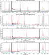 |
Fig. 3. Some examples of SDSS-V spectra fitted using the NBURSTS full-spectrum fitting technique with E-MILES SSP models and double emission line templates (narrow and broad). Four spectra with a high S/N in continuum (> 20), which allows a reliable identification of the narrow and broad components, were selected for demonstration. The broad-line component is clearly visible and robustly detected in multiple Balmer series lines. This confirms the BLR alongside the NLR. The central panels show the spectrum in the full available wavelengths range, and the side panels show the surrounding ranges of two spectral lines Hβ and Hα. The black line corresponds to spectrum fluxes, the red line shows a best-fit model, the purple line shows a stellar population model including multiplicative continuum (stellar component), the dark blue line shows an additive component that describes the AGN continuum, and the light blue and green lines show emission line templates for narrow and broad lines, respectively. The dark gray line shows the residuals, and the light gray areas show masked regions that were excluded from the fit. |
3.2. Black hole mass estimates
By decomposing the permitted emission lines into broad and narrow components, we estimated a single-epoch black hole mass (MBH) using a virial approximation applied to a broad Hα emission line (Reines et al. 2013). This method assumes that the gas in the BLR is virialized and its motions are driven by the gravitational influence of the black hole. The virial mass was calculated using the velocity dispersion of the gas, which was derived from the width, full width at half maximum, of the broad Hα line, and the radius of the BLR, which was inferred from empirical scaling relations based on the luminosity of the broad Hα emission using the following equation:
![Mathematical equation: $$ \begin{aligned} \log&\left( \frac{M_{\mathrm{BH}}}{M_{\odot }} \right)&= 6.57 + 0.47 \log \left( \frac{L_{\mathrm{H}\alpha }^{\mathrm{BLR}}}{10^{42} [\mathrm{erg}\, \mathrm{s}^{-1}]} \right) + 2.06 \log \left( \frac{\mathrm{FWHM}_{\mathrm{H}\alpha }^{\mathrm{BLR}}}{10^3 [\mathrm{km}\, \mathrm{s}^{-1}]} \right), \end{aligned} $$](/articles/aa/full_html/2025/10/aa55117-25/aa55117-25-eq5.gif) (4)
(4)
where the coefficients derived by Reines et al. (2013) were adopted from the RHβ − L5100 relation (Bentz et al. 2013) and the FWHMHβ − FWHMHα, LHα − L5100 relations were adopted from Greene & Ho (2005).
For the subsample of spectra with reliable broad-line component detections (S/N > 3 in broad Hα, σbroad > 1.5 σnarrow and σbroad is in range from 300 to 5000 km/s, QUALITY = 2; see Sect. 4.1, and Fig. 2), we estimated the black hole masses. We considered the measurement uncertainties of  and broad Hα flux returned by the NBURSTS code, which we propagated to estimate the MBH uncertainties.
3.3. Fitting of empirical power-law relations
To fit the empirical relations between parameters [LX versus LOIII] as power laws, we used the nested-sampling algorithm (Skilling 2004; Buchner 2023) implemented in the Python package ULTRANEST (Buchner 2021). The likelihood is the line (in log space) with slope, offset, and intrinsic scatter, and the priors are normal distributions. The posteriors for slope, offset, and intrinsic scatter for the LX(LOIII) relation are available on Zenodo (Demianenko & Pulatova 2025)3. The graphs with linear fits through the paper represent ordinary least-squares fits.
4. Results
4.1. Main results and subsamples
The final fitting results for 7546 spectra of 3684 sources from the SDSS-V DR19 eROSITA eRASS1 X-ray-selected galaxies sample in the 0.002 < z < 0.55 range are presented in a table that is available at the CDS (see Appendix A for the column description). The table contains lists of the main emission lines in the rest-frame wavelength range 3700−7000 Å from [O II]λ3727 to [S II]λ6731: 28 lines for the narrow component, and 6 lines of the Balmer series (from H8 to Hα) for the broad component. The absence of any line identifier in the specified wavelength range in the list of lines does not necessarily indicate its absence in each individual spectrum. A total of 140 lines fell within the fitting ranges, from which we selected 34 lines for the final compiled table that occurred in spectra most frequently. X-ray fluxes at different energies from eRASS1 based on our cross-match were included in the table. Finally, we included quality flags for the fitting results based on the set of parameters obtained (see the QUALITY field), which can take four values according to the following filters:
-
0:
A subsample with a reliable detection of a narrow component comprising at least three forbidden unblended emission lines with S/N > 3 (e.g. [O III] and [O II]) and fulfilling the kinematic constraints 50 < σnarrow < 1000 km/s and Δσnarrow < 300 km/s.
-
1:
A subsample of (0) for the BPT diagram classification with additional conditions of S/N > 3 in each of the following lines: Hα, Hβ, [N II]λλ6548, 84, and [O III]λ5007.
-
2:
A subsample of (1) with a reliable detection of a broad component:
 and σbroad > 1.5 σnarrow, 300 < σbroad < 5000 km/s, and Δσbroad < 300 km/s.
 -
-1:
All other spectra that did not fall into any of the above categories were marked as unreliable.
In the final subsamples (i) with QUALITY = 0, we have 5898 spectra of 3058 sources with reliable measurement of narrow-line properties [2844 of these have broad lines detected according to the criteria stated in (2)]; (ii) with QUALITY = 1, we have 4698 spectra of 2487 sources that are suitable for the BPT classification; (iii) with QUALITY = 2, we have 4388 spectra of 2343 sources with a reliable detection of a broad component and suitable for black hole mass estimates (the method is described in Sect. 3.2); (iv) the remaining 1648 spectra of 1130 sources have QUALITY = −1. We remark that this final subset is not completely hopeless; they may be useful for other tasks related to the study of individual emission line properties, but this requires an appropriate selection of additional criteria for emission line measurements.
The sequence in which we obtained the subsamples is depicted in Fig. 2. For further diagnostics and to verify the dependences, we focus herein on a subsample of sources with the QUALITY = 2 flag as the most reliable candidates with sufficient signal (S/N > 3) in the main broad and NELs. For users interested in analyzing sources with a broader range of spectral quality, the selection criterion QUALITY > 0 can be used to include all objects with acceptable (nonzero) spectral classifications.
4.2. Emission line comparison with previous surveys
To validate our results for measurements of optical emission line fluxes, we compared them with previously published fluxes from RCSED (Chilingarian et al. 2017) and SDSS-IV DR17 (Blanton et al. 2017). The RCSED project is based on the analysis of SDSS DR7 spectra using an earlier version of the NBURSTS code without emission line decomposition. The SDSS-IV DR17 catalog also provides emission line fluxes without decomposition into narrow and broad components. To perform this test, we cross-matched these catalogs with the QUALITY = 2 flag X-ray sample using TOPCAT with an angular separation of 1″ and requiring S/N > 3 in the emission lines. We found 101 and 75 sources in the two groups, respectively. It agreed well with SDSS-IV DR17 data and was correlated with RCSED (see Fig. 4 Sect. 4.2)
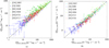 |
Fig. 4. Comparison of fluxes in forbidden optical emission lines obtained with the NBURSTS technique for X-ray-selected DR19 galaxies (x-axis, this paper) with previously published results (y-axis). The left panel compares 101 galaxies in common with the RCSED catalog (Chilingarian et al. 2017). The right panel compares 75 galaxies in common with the RCSED SDSS DR17 data release (Blanton et al. 2017). The dashed black line represents the 1:1 relation. The fluxes we obtained agree well with SDSS-IV DR17 data and are correlated with RCSED. |
As a further comparison, we examined the BPT diagram locations in Fig. 5 for RCSED (base of the arrow), where no decomposition is made, and our line fluxes (top of the arrow), where narrow and broad components were decomposed. The decomposition shifts the sources on the BPT diagram upward along the log[O III]/Hβ axis in 82% of cases, and only 18% are shifted downward, with a median shift of +0.17 dex and a 16–84% percentile range of [+0.07, +0.38] dex. The analysis highlights the importance of the decomposition in accurately identifying whether the ionization mechanism is dominated by AGNs or star formation and in preventing misclassifications that arise when broad components from the AGNs are included in the total flux. We note that the broad component can be detected not only by the presence of a type-I AGN, but also by high-velocity galactic winds, associated shocks (Shapiro et al. 2009), or internal kinematics, such as bars (Pulatova et al. 2015).
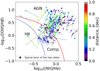 |
Fig. 5. Change in the position in the BPT diagram for 101 galaxies of the matched sample from this work with the RCSED catalog. At the base of the arrow is the position determined by the emission line fluxes from the RCSED without decomposition, and at the top of the arrow is the position determined by the narrow component as a result of decomposition into narrow and broad components. The color code denotes the distance between the two measures in the diagram. |
4.3. BPT diagrams
After demonstrating the advantages of the line decomposition for isolating AGN dominant components, we now investigate potential trends across the BPT of X-ray-selected galaxies among several parameters of interest (color-coded symbols) as described below.
-
Figure 6a is color-coded by X-ray-to-Hα flux ratio. This allows us to confirm and strengthen the correlation found by Pulatova et al. (2024), Fig. 6a. The X-ray to Hα flux ratio in the BPT diagram for AGNs in the sample by Pulatova et al. (2024) (FX-ray/FHα > 1) and the current eRASS1 sample (FX-ray/FHα > 2) is also shown. The higher FX-ray/FHα ratio for AGNs in the current work can be explained by the fact that for the eRASS1 sample, the line fluxes arise only from the NEL component, while Pulatova et al. (2024) used the total Hα fluxes without decomposition (Sect. 5).
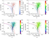
Fig. 6. BPT diagram for X-ray-selected galaxies. The color codes show the ratio of X-ray [0.2 − 2.4 keV] to Hα (panel a), the black hole mass (panel b), the σnarrow, km s−1 (panel c), and the X-ray luminosity in 0.2 − 2.3 keV (panel d).
-
Figure 6b is color-coded by single-epoch SMBH mass estimates, illustrating that the SMBH mass correlates with the position of a galaxy on the BPT diagram. Galaxies with SMBH masses > 108 M⊙ are mainly located in the upper part of the loci of Seyfert and low-ionization nuclear emission-line regions (LINERs) in the BPT diagram. Galaxies with lower-mass SMBHs are more often located at the bottom of the Seyfert and LINERs loci, however.
-
Figure 6c is color-coded by the velocity dispersion (σnarrow) of the NEL component to reflect the dynamics of the NLR gas and its role in influencing the position of a galaxy on the BPT diagram. Galaxies with higher σnarrow are located at the top of the diagram.
-
Figure 6d is color-coded by the X-ray luminosity (L0.2 − 2.3 keV). Against expectations, there is no strong trend from the HII to AGN regions. Nevertheless, galaxies with X-ray luminosities below 1041 erg s−1 are predominantly located in the bottom part of LINERs, suggesting that AGNs with low X-ray luminosities are more likely associated with weaker ionization mechanisms. This highlights the complexity of the AGN-host galaxy interactions and the need for multiwavelength approaches to understand these systems better.
A similar optical study using SDSS-V AGN data, including the WHaN (Width of Hα and the [N II]/Hα line ratio) diagram, was presented by Cortes-Suárez et al. (2022). The authors emphasized the challenges of measuring NELs in spectra that are dominated by intense broad-line emission, where the narrow components may be partially blended or suppressed.
4.4. X-ray [0.2–2.3] keV and optical lines luminosities
In Fig. 7 we compare the broad- and narrow-line luminosities for Hα (a) and Hβ (b). The eROSITA X-ray luminosity (0.2 − 2.3 keV range) is color-coded. No significant difference between Hα and Hβ is detected. The X-ray luminosity correlates with the broad and narrow components of these Balmer lines, and the trends are consistent. One notable difference is the relative flux contribution, which we explain below: For the majority of galaxies in our sample, the flux in the broad component is higher than that in the corresponding narrow component. This trend is clearly visible in Fig. 7, where most data points lie above the one-to-one line (x = y). Only a small fraction of sources show the opposite behavior and the narrow component dominates the broad component. We also note that at lower X-ray fluxes, a larger fraction of the Balmer narrow-line emission may originate from star formation in the host galaxy than from AGN photoionization. This is especially relevant in systems with a modest or obscured AGN contribution to the total ionizing budget. In these cases, the narrow components may reflect H II region emission and not excitation from the AGN NLR, which contributes to additional scatter in the correlation between narrow-line luminosity and X-ray emission. This trend is consistent with previous findings (Kauffmann et al. 2003; Ho 2008). The correlations in Fig. 7 are physically motivated. The broad components originate in the BLR, which lies very close to the central SMBH and is directly exposed to the ionizing continuum. In contrast, the narrow components are produced in the more extended NLR, where the local gas density, obscuration, and ionization geometry can vary significantly. The consistent correlations for the two components suggest that despite the differences in the spatial scale and the physical conditions, the optical emission lines still reflect the strength of the central ionizing source.
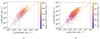 |
Fig. 7. Optical luminosity in the broad and narrow components. The color code shows the eROSITA X-ray luminosity in 0.2 − 2.3 keV. The dashed black line represents the 1:1 relation. It demonstrates a strong connection between the BLR, NLR, and the X-ray source. Panel a shows Hα, and panel b shows Hβ. |
To further explore the physical connection between X-ray emission and ionized gas properties, Fig. 8 shows the correlation between X-ray luminosity in the 0.2–2.3 keV band and the luminosities of two prominent emission lines: Hα (broad component; panel a) and [O III] λ5007 (panel b). The stellar velocity dispersion (σ*) is color-coded in both panels. These emission-line luminosities are often used as observational tracers of AGN activity, but they are affected by the ionizing UV continuum and the structure of the emitting regions. Similar correlations were discussed before (Panessa et al. 2006), and our results extend this picture for a uniformly selected eRASS1 sample. These panels reveal a strong correlation between X-ray luminosity and the broad component of Hα and [O III], which reinforces the close connection of these two emissions to the central engine of the AGN. The best linear correlations are expressed as
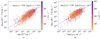 |
Fig. 8. Correlations between the X-ray [0.2 − 2.3 keV], broad Hα (a), and narrow [O III] (b) luminosities. The color-coding represents the velocity dispersion of the stellar component and links the kinematics to the AGN activity. The dashed lines and equations near the top of the panel denote the best-fit correlations. The uniform scaling between the X-ray and line luminosities reinforces their common AGN origin. |
 (5)
(5)
and
![Mathematical equation: $$ \begin{aligned} \log L_{\rm X} = (0.68 \pm 0.02) \cdot \log \mathrm{[OIII]} + (14.41 \pm 0.59). \end{aligned} $$](/articles/aa/full_html/2025/10/aa55117-25/aa55117-25-eq9.gif) (6)
(6)
The correlations presented in Equations (5) and (6) are consistent with physical models of the AGN structure and emission mechanisms. Specifically, the correlation between X-ray and [O III] luminosities reflects the ionization of NLR gas by high-energy photons from the accretion disk and corona (Heckman & Best 2014; Panessa et al. 2006; Ueda et al. 2015). The similar correlation observed between X-ray and broad Hα luminosity arises from photoionization of the BLR, which is located in the immediate vicinity of the SMBH and is directly illuminated by the ionizing continuum (Panessa et al. 2006; Imanishi & Ueno 1999). These approximations yield identical coefficients 0.68 ± 0.06 (slope) and ≈15 ± 0.59 (intercept) and indicate that the X-ray luminosity scales uniformly with the optical luminosities of the Hα broad component and the [O III] emission lines. The identical coefficients suggest that the physical processes governing the generation of X-ray and optical, BEL, and NEL emissions are closely linked, regardless of the emission line that is used. This similar scaling for Hα (broad component) and [O III] (narrow component) suggests a physical connection between the central AGN activity, which powers the X-ray emission, and the ionized gas in the BLR and NLR.
Figure 9 shows the relation between X-ray luminosity (0.2 − 2.3 keV) and SMBH mass for X-ray galaxies. The stellar velocity dispersion is color-coded. As expected, the X-ray luminosity increases in general with SMBH mass. This largely reflects the underlying M–σ relation and its intrinsic scatter (e.g., Tremaine et al. 2002; Kormendy & Ho 2013). It demonstrates that a higher X-ray luminosity tends to be associated with more massive SMBHs, which agrees with the understanding that more massive SMBHs have higher absolute accretion rates on average. The distribution of the Eddington rates is folded into this correlation, however, and we plan to consider additional selection effects, in particular, with distance, in future studies. For example, the X-ray luminosities of small central black holes in the intermediate-mass regime (Reines et al. 2013; Chilingarian et al. 2018) sometimes lie in the range 1042 − 1043 erg s−1. The best-fitting linear regression has the form
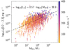 |
Fig. 9. Mass diagram of the X-ray luminosity and the SMBH. The color code shows the velocity dispersion of the stellar component σ*. |
 (7)
(7)
These results highlight the strong interplay between the X-ray output and the black hole mass and reinforce the connection between the AGN central activity and its observable properties in the optical and X-ray wavelengths.
5. Discussion
5.1. eROSITA and XMM-Newton samples
A major difference in the approach to defining the galaxy samples in this work and in Pulatova et al. (2024) lies in the differences between the XMM-Newton and eROSITA missions. The eROSITA survey covers the entire sky, and the pointed observations of XMM-Newton only cover ≈3% with a large range in sensitivity. The positional accuracy of XMM-Newton source detections is much better than in eROSITA, however. On the other hand, eROSITA observations enable us to study broader and more distant samples of the galaxy populations (Fig. 1b). Our sample benefits from the SDSS-V SPIDERS target list, which employs probabilistic associations. The adopted selection method (based on NWAY and a machine-learning classification) optimally balances positional accuracy with the multiwavelength source properties and achieved high completeness and reliability.
For faint sources, eROSITA X-ray fluxes may appear to be systematically higher than those reported by deeper surveys such as XMM-Newton, particularly in the soft energy band. This might be related to ongoing calibration uncertainties in eRASS1, especially below 1 keV. A detailed comparison and discussion of the flux calibration between eROSITA, 4XMM, and Chandra was provided by Merloni et al. (2024a), who analyzed and quantified these systematic effects.
We here only used the narrow component of the Hα emission line, while Pulatova et al. (2024) used the total fluxes without a decomposition for the BPT. A decomposition systematically results in lower narrow-line fluxes than total fluxes because it isolates the AGN contribution by removing contamination from the broad-line component and the host galaxy light. This reduction in the Hα flux further increases the X-ray/Hα flux ratio in the eROSITA sample.
These differences highlight the importance of consistent methods when AGN diagnostics are compared for different datasets.
5.2. Classification of galaxies with an AGN
An AGN can be detected by several complementary approaches, including diagnostics such as the optical BPT (Baldwin et al. 1981) or WHaN (Cid Fernandes et al. 2011) diagrams, broad-band optical or infrared variability (Wang et al. 2024), X-ray detection with the luminosity exceeding that from the stellar population (Merloni et al. 2014; Fitriana & Murayama 2022), or gamma-ray and radio emission (Dermer & Giebels 2016). In general, the X-ray selection of AGNs is more effective than an optical selection because it is less affected by obscuration from intervening material and is less prone to contamination by the light from the host galaxy, which can dilute AGN signals at optical wavelengths (Hickox & Alexander 2018; Grishin et al. 2025). The BPT diagram uses emission-line ratios ([O III]/Hβ versus [N II]/Hα) to distinguish AGNs from star-forming galaxies by identifying ionization mechanisms consistent with AGNs. This method can be affected by aperture effects, dust attenuation, and the requirement for the detection of emission lines, however. Therefore, the most reliable candidates for galaxies with active nuclei are obtained when several of the listed criteria are met simultaneously.
We applied a strict criterion of S/N > 3 for optical emission lines (Hα, Hβ, [O III], [N II] – QUALITY > 1) to ensure more reliable results but to reduce the sample size significantly. Lowering the S/N threshold allows more AGN candidates with weak emission lines, which are missing from the current sample. For comparison, Pucha et al. (2025) used S/N > 3 for [O III], Hα, and [N II], but a lower threshold of S/N > 1 for Hβ, and acknowledged its weaker detectability in many galaxies. Similarly, Ryzhov et al. (2025) applied S/N > 2 and noted that increasing the threshold to S/N > 3 had little impact on their conclusions, but reduced the number of classified galaxies, particularly those with weak AGNs or star-forming activity. This trade-off underscores the importance of carefully selecting S/N criteria to balance reliability and sample completeness.
Our current study confirms the dependence of the galaxy position in the BPT diagram on its X-ray/Hα ratio from Pulatova et al. (2024). This result agrees with previous studies of the connection between X-ray and optical emission. The logarithm of the X-ray-to-optical(continuum) flux ratio > − 1 was used to identify AGNs in their host galaxies (Brandt & Hasinger 2005; Fitriana & Murayama 2022). A correlation has been established between the soft X-ray luminosities and Hα luminosities (Elvis et al. 1984; Koratkar et al. 1995; Halderson et al. 2001). Compared to its significant influence in the optical spectrum, the relatively minor contribution of the host galaxy to X-ray emission enhances the reliability of X-ray observations as a method for identifying AGNs.
5.3. X-ray and optical luminosities, and the estimation of the SMBH
We only considered sources with QUALITY = 2, which corresponds to spectra with reliable optical emission-line measurements. While this ensured consistency in the derived trends with X-ray fluxes, it also introduced a selection bias. A substantial number of X-ray–detected sources with lower-quality spectral classification (many of which may be type I AGNs with weak or undetected optical lines) were excluded. These objects might influence the observed flux–flux correlations.
Georgantopoulos & Akylas (2010) compared the efficiency of X-ray and [O III] optical luminosity functions for identifying AGNs and discussed the dependence of the X-ray and [O III] luminosities. The slopes and intercepts they obtained were different for different types of Seyfert galaxies, from 0.59 to 1.04 and from −0.17 (Seyfert 1) to 16.15, correspondingly. For the X-ray DR19 sample, we obtained a slope of 0.68 and an intercept of 15. These numbers agree with the data for Seyfert 2 and luminous Seyfert 1 galaxies (Georgantopoulos & Akylas 2010). Panessa et al. (2006) reported a slope and intercept for their LX − L[OIII] diagram of 1.22 and −7.34, respectively, which differ from our work. We attribute the observed scatter to a combination of factors, including the sample selection, methodological differences, and intrinsic physical diversity within the AGN population.
The LX − L[OIII] relation was also studied by Agostino et al. (2023) based on a sample of 500 low-redshift AGNs observed by XMM-Newton and SDSS. They showed that so-called optically dull AGNs are not a distinct class, but instead represent the [O III]-under-luminous tail of the unimodal LX − L[OIII] relation. Their analysis further revealed that the degree of [O III] under-luminosity correlates with the host galaxy properties, particularly the specific star formation rate. This suggests that the observed scatter in the relation is affected by host-driven effects and not by intrinsic AGN differences.
The MBH − σ* scaling relation (Ferrarese & Merritt 2000; Gebhardt et al. 2000) links SMBH mass (MBH) with the velocity dispersion of stars in galaxy bulges. This has been a cornerstone of understanding black hole growth and black hole – host coevolution (Kormendy & Ho 2013). Figure 9 shows the close connection between σ*, MBH, and LX, the linear fit of which yielded slope and intercept coefficients 0.57 and 38.9, respectively. These values agree with previous research, where a correlation was found between the BH mass and luminosity (Kollmeier et al. 2006). Panessa et al. (2006), however, observed no direct correlation between LX and MBH for the sample of 47 local SMBHs based on data from Chandra, XMM-Newton, and Advanced Satellite for Cosmology and Astrophysics (ASCA) observations.
6. Conclusions
We analyzed the X-ray and optical properties of galaxies selected from the SDSS-V/SPIDERS program. The sample was based on the counterparts to eROSITA X-ray sources that were identified using the NWAY algorithm with machine-learning techniques, as described by Salvato et al. (2022) and Salvato & Wolf (2025).
Our main findings and conclusions are listed below.
-
We created a new sample of X-ray-selected galaxies (see Sect. 2.2) and applied the NBURSTS technique to analyze 7546 SDSS-V optical spectra of 3684 sources (see Sect. 4.1 and Appendix A for table description). To ensure the reliability of our results, we applied specific kinematic and S/N criteria to the dataset and examined the properties of the high-quality subsample (QUALITY = 2; see Sect. 4.1).
-
We compared the narrow forbidden emission line fluxes with the published catalogs RCSED and SDSS-IV DR17. The fluxes agreed well with SDSS-IV DR17 data and correlated with RCSED (see Fig. 4 Sect. 4.2).
-
With the QUALITY = 2 subsample, we showed that the narrow and broad decomposition of optical emission lines is crucial for the diagnostic BPT diagrams, which rely on the flux ratios of narrow-line emission (e.g., [O III]/Hβ and [N II]/Hα) to classify galaxies into star-forming, Seyfert, LINERs, or composite categories. This leads to a shift in the position in the BPT diagram. We found that 82% of galaxies moved upward along the log([O III]/Hβ) axis, with a median shift of +0.17 dex and a 16–84% percentile range of [+0.07, +0.38] dex. This upward shift reflects a more precise representation of the AGN ionization mechanism by isolating the narrow-line components that are less affected by contamination from the broad component and stellar contributions from the host galaxy.
-
We demonstrated a clear and consistent correlation between the X-ray luminosity and the luminosities of both the broad and narrow components of permitted emission lines (Hα and Hβ), as well as with the narrow forbidden [O III] line (see Sect. 4.4, Figs. 7 and 8). The broad-line luminosities trace the immediate vicinity of the SMBH, where the gas dynamics are dominated by the central AGN, while the narrow-line components probe ionized gas on larger galactic scales. These correlations suggest a common physical driver, namely, the AGN UV accretion disk emission, which powers the ionized gas and the high-energy X-rays. Although the UV continuum is difficult to observe directly, the slopes and scatter of the optical-X-ray relations offer valuable insights into how this radiation is reprocessed by various AGN structures and into the role of geometry, covering factor, and ionization state. The nearly identical correlation coefficients found for the broad Hα and narrow [O III] lines (both with slopes of 0.68 and similar intercepts) indicate that the X-ray luminosity scales uniformly with the optical line emission. This reinforces its role as a robust tracer of the AGN activity in different spatial regions and for different emission mechanisms.
-
We confirmed the dependence of the position in the BPT diagram as a function of X-ray/Hα ratio as reported by Pulatova et al. (2024) using decomposed narrow-line fluxes. This extended the trend to higher X-ray/Hα flux ratios (FX − ray/FHα > 2) (see Sect. 4.3 and Fig. 6a).
-
We demonstrated correlations between the position of a source in the BPT diagram and the main galaxy parameters (see Fig. 6), including the black hole mass (MBH) and velocity dispersion (σnarrow). Galaxies with higher MBH and σnarrow values are systematically located higher on the log([O III]/Hβ) axis, indicating a more substantial AGN ionization contribution. This trend underscores the connection between the central black hole properties and the ionization state of the NLR. In future work, we plan to explore several open questions in more detail. For example, we aim to apply completeness corrections based on the full SDSS-V selection function and to model selection biases more quantitatively using mock catalogs. A more detailed investigation of the physical drivers behind the observed emission-line correlations (e.g., black hole mass, Eddington ratio, and host galaxy properties) also remains to be done. Additionally, we intend to include diagnostic tools such as the WHaN diagram (Cid Fernandes et al. 2011) to better separate AGNs from star formation contributions in the NELs. These directions will help us to refine the interpretation of emission-line scaling relations and further constrain the coevolution of AGNs and their host galaxies.
Data availability
Table A.1, which contains the results presented in this paper, is only available at the CDS via https://cdsarc.cds.unistra.fr/viz-bin/cat/J/A+A/702/A67. A detailed description of the table columns is provided in Table A.1. The posteriors for LX-LOIII scaling relation are available on Zenodo (Demianenko & Pulatova 2025).
Acknowledgments
Funding for the Sloan Digital Sky Survey V (SDSS-V) has been provided by the Alfred P. Sloan Foundation, the Heising-Simons Foundation, the National Science Foundation, and the participating institutions. SDSS-V is managed by the Astrophysical Research Consortium for the Participating Institutions of the SDSS Collaboration. For a full list of SDSS-V participating institutions, please see https://www.sdss.org/ We are grateful to all contributors who have enabled SDSS-V’s scientific capabilities. Part of this work was supported by the German Deutsche Forschungsgemeinschaft, DFG, Water Benjamin Stelle, project number PU 848/1–1. Igor Chilingarian’s research is supported by the Telescope Data Center at the Smithsonian Astrophysical Observatory. He also acknowledges the support from the NASA ADAP-22-0102 grant (award 80NSSC23K0493). ER and DG’s research on the analysis and fitting of spectra was supported by the Russian Science Foundation (RScF) grant No. 23-12-00146. C. Aydar acknowledges the support by the Excellence Cluster ORIGINS, which is funded by the Deutsche Forschungsgemeinschaft (DFG, German Research Foundation) under Germany’s Excellence Strategy – EXC-2094 – 390783311. MD expresses gratitude to the International Max Planck Research School for Astronomy and Cosmic Physics at the University of Heidelberg (IMPRS-HD). Nadiia Pulatova is grateful for the scientific discussion to Anatolii Tugay, Lidiia Zadorozhna; and for IT support to Stefan Kallweit; and for inspiration to Emiliia Pulatova. RJA was supported by FONDECYT grant number 1231718 and by the ANID BASAL project FB210003. FEB acknowledges support from ANID-Chile BASAL CATA FB210003, FONDECYT Regular 1241005, and Millennium Science Initiative, AIM23-0001. CAN and HJIM acknowledge the support from projects CONAHCyT CBF2023-2024-1418, PAPIIT IA104325 and IN119123. This research made use of TOPCAT, a software tool for astronomical data analysis (Taylor 2005). We acknowledge Mark Taylor for developing and maintaining this valuable resource. We acknowledge the use of ChatGPT, Grammarly, and DeepL for language refinement and improving the manuscript’s clarity. The final content remains the responsibility of the authors. We complement the use of LLMs with critical thinking, as was proposed in Fouesneau et al. (2024).
References
- Abdurro’uf, Accetta, K., Aerts, C., et al. 2022, ApJS, 259, 35 [NASA ADS] [CrossRef] [Google Scholar]
- Agostino, C. J., Salim, S., Ellison, S. L., Bickley, R. W., & Faber, S. M. 2023, ApJ, 943, 174 [NASA ADS] [CrossRef] [Google Scholar]
- Allen, M. G., Groves, B. A., Dopita, M. A., Sutherland, R. S., & Kewley, L. J. 2008, ApJS, 178, 20 [Google Scholar]
- Antonucci, R. 1993, ARA&A, 31, 473 [Google Scholar]
- Aydar, C., Merloni, A., Dwelly, T., et al. 2025, A&A, 698, A132 [NASA ADS] [CrossRef] [EDP Sciences] [Google Scholar]
- Baldwin, J. A., Phillips, M. M., & Terlevich, R. 1981, PASP, 93, 5 [Google Scholar]
- Bentz, M. C., Denney, K. D., Grier, C. J., et al. 2013, ApJ, 767, 149 [Google Scholar]
- Blanton, M. R., Bershady, M. A., Abolfathi, B., et al. 2017, AJ, 154, 28 [Google Scholar]
- Brandt, W. N., & Hasinger, G. 2005, ARA&A, 43, 827 [NASA ADS] [CrossRef] [Google Scholar]
- Buchner, J. 2021, J. Open Source Softw., 6, 3001 [CrossRef] [Google Scholar]
- Buchner, J. 2023, Statistics Surveys, 17, 169 [Google Scholar]
- Cappellari, M. 2017, MNRAS, 466, 798 [Google Scholar]
- Chilingarian, I. V., & Asa’d, R. A. 2018, ApJ, 858, 63 [NASA ADS] [CrossRef] [Google Scholar]
- Chilingarian, I., Prugniel, P., Sil’chenko, O., & Koleva, M. 2007a, in Stellar Populations as Building Blocks of Galaxies, eds. A. R. Vazdekis, & R. Peletier, IAU Symp., 241, 175 [Google Scholar]
- Chilingarian, I. V., Prugniel, P., Sil’Chenko, O. K., & Afanasiev, V. L. 2007b, MNRAS, 376, 1033 [NASA ADS] [CrossRef] [Google Scholar]
- Chilingarian, I. V., Zolotukhin, I. Y., Katkov, I. Y., et al. 2017, ApJS, 228, 14 [NASA ADS] [CrossRef] [Google Scholar]
- Chilingarian, I. V., Katkov, I. Y., Zolotukhin, I. Y., et al. 2018, ApJ, 863, 1 [Google Scholar]
- Chilingarian, I., Borisov, S., Goradzhanov, V., et al. 2024, in Astromical Data Analysis Software and Systems XXXI, eds. B. V. Hugo, R. Van Rooyen, & O. M. Smirnov, ASP Conf. Ser., 535, 179 [Google Scholar]
- Cid Fernandes, R., Stasińska, G., Mateus, A., & Vale Asari, N. 2011, MNRAS, 413, 1687 [Google Scholar]
- Comparat, J., Merloni, A., Salvato, M., et al. 2019, MNRAS, 487, 2005 [Google Scholar]
- Cortes-Suárez, E., Negrete, C. A., Hernández-Toledo, H. M., Ibarra-Medel, H., & Lacerna, I. 2022, MNRAS, 514, 3626 [Google Scholar]
- Demianenko, M., & Pulatova, N. 2025, Posteriors for LX-LOIII [Google Scholar]
- Dermer, C. D., & Giebels, B. 2016, Comptes Rendus Physique, 17, 594 [NASA ADS] [CrossRef] [Google Scholar]
- Dey, A., Schlegel, D. J., Lang, D., et al. 2019, AJ, 157, 168 [Google Scholar]
- Dwelly, T., Salvato, M., Merloni, A., et al. 2017, MNRAS, 469, 1065 [Google Scholar]
- Elvis, M., Soltan, A., & Keel, W. C. 1984, ApJ, 283, 479 [NASA ADS] [CrossRef] [Google Scholar]
- Fabian, A. C. 2012, ARA&A, 50, 455 [Google Scholar]
- Ferland, G. J., & Netzer, H. 1983, ApJ, 264, 105 [NASA ADS] [CrossRef] [Google Scholar]
- Ferrarese, L., & Merritt, D. 2000, ApJ, 539, L9 [Google Scholar]
- Fitriana, I. K., & Murayama, T. 2022, PASJ, 74, 689 [NASA ADS] [CrossRef] [Google Scholar]
- Fouesneau, M., Momcheva, I. G., Chadayammuri, U., et al. 2024, ArXiv e-prints [arXiv:2409.20252] [Google Scholar]
- Gebhardt, K., Bender, R., Bower, G., et al. 2000, ApJ, 539, L13 [Google Scholar]
- Georgantopoulos, I., & Akylas, A. 2010, A&A, 509, A38 [NASA ADS] [CrossRef] [EDP Sciences] [Google Scholar]
- Giacconi, R., Gursky, H., Paolini, F. R., & Rossi, B. B. 1962, Phys. Rev. Lett., 9, 439 [NASA ADS] [CrossRef] [Google Scholar]
- Goradzhanov, V., Chilingarian, I., Rubtsov, E., et al. 2024, in Astromical Data Analysis Software and Systems XXXI, eds. B. V. Hugo, R. Van Rooyen, & O. M. Smirnov, ASP Conf. Ser., 535, 175 [Google Scholar]
- Greene, J. E., & Ho, L. C. 2005, ApJ, 630, 122 [NASA ADS] [CrossRef] [Google Scholar]
- Grishin, K. A., Chilingarian, I. V., Combes, F., et al. 2025, A&A, in press, https://www.doi.org/10.1051/0004-6361/202554130 [Google Scholar]
- Halderson, E. L., Moran, E. C., Filippenko, A. V., & Ho, L. C. 2001, AJ, 122, 637 [Google Scholar]
- Harrison, C. M., Alexander, D. M., Swinbank, A. M., et al. 2012, MNRAS, 426, 1073 [NASA ADS] [CrossRef] [Google Scholar]
- Heckman, T. M., & Best, P. N. 2014, ARA&A, 52, 589 [Google Scholar]
- Hickox, R. C., & Alexander, D. M. 2018, ARA&A, 56, 625 [Google Scholar]
- Ho, L. C. 2008, ARA&A, 46, 475 [Google Scholar]
- Imanishi, M., & Ueno, S. 1999, MNRAS, 305, 829 [Google Scholar]
- Kauffmann, G., Heckman, T. M., Tremonti, C., et al. 2003, MNRAS, 346, 1055 [Google Scholar]
- Kewley, L. J., & Dopita, M. A. 2002, ApJS, 142, 35 [Google Scholar]
- Kewley, L. J., Groves, B., Kauffmann, G., & Heckman, T. 2006, MNRAS, 372, 961 [Google Scholar]
- Klochkov, V., Katkov, I., Chilingarian, I., et al. 2024, in Astromical Data Analysis Software and Systems XXXI, eds. B. V. Hugo, R. Van Rooyen, & O. M. Smirnov, ASP Conf. Ser., 535, 243 [Google Scholar]
- Koleva, M., Prugniel, P., Ocvirk, P., Le Borgne, D., & Soubiran, C. 2008, MNRAS, 385, 1998 [NASA ADS] [CrossRef] [Google Scholar]
- Kollmeier, J. A., Onken, C. A., Kochanek, C. S., et al. 2006, ApJ, 648, 128 [NASA ADS] [CrossRef] [Google Scholar]
- Kollmeier, J., Anderson, S. F., Blanc, G. A., et al. 2019, Bull. Am. Astron. Soc., 51, 274 [Google Scholar]
- Kollmeier, J. A., Rix, H. W., Aerts, C., et al. 2025, Sloan Digital Sky Survey-V: Pioneering Panoptic Spectroscopy [Google Scholar]
- Kollmeier, J. A., Zasowski, G., Rix, H. W., et al. 2017, ArXiv e-prints [arXiv:1711.03234] [Google Scholar]
- Koratkar, A., Deustua, S. E., Heckman, T., et al. 1995, ApJ, 440, 132 [NASA ADS] [CrossRef] [Google Scholar]
- Kormendy, J., & Ho, L. C. 2013, ARA&A, 51, 511 [Google Scholar]
- Markwardt, C. B. 2009, in Astronomical Data Analysis Software and Systems XVIII, eds. D. A. Bohlender, D. Durand, & P. Dowler, ASP Conf. Ser., 411, 251 [Google Scholar]
- Merloni, A., Bongiorno, A., Brusa, M., et al. 2014, MNRAS, 437, 3550 [Google Scholar]
- Merloni, A., Lamer, G., Liu, T., et al. 2024a, A&A, 682, A34 [NASA ADS] [CrossRef] [EDP Sciences] [Google Scholar]
- Merloni, A., Lamer, G., Liu, T., et al. 2024b, VizieR Online Data Catalog: SRG/eROSITA all-sky survey catalogs (eRASS1) [Google Scholar]
- Osterbrock, D. E., & Ferland, G. J. 2006, Astrophysics of Gaseous Nebulae and Active Galactic Nuclei (University Science Books) [Google Scholar]
- Panessa, F., Bassani, L., Cappi, M., et al. 2006, A&A, 455, 173 [NASA ADS] [CrossRef] [EDP Sciences] [Google Scholar]
- Planck Collaboration VI. 2020, A&A, 641, A6 [NASA ADS] [CrossRef] [EDP Sciences] [Google Scholar]
- Predehl, P., Andritschke, R., Arefiev, V., et al. 2021, A&A, 647, A1 [EDP Sciences] [Google Scholar]
- Pucha, R., Juneau, S., Dey, A., et al. 2025, ApJ, 982, 10 [Google Scholar]
- Pulatova, N. G., Vavilova, I. B., Sawangwit, U., Babyk, I., & Klimanov, S. 2015, MNRAS, 447, 2209 [Google Scholar]
- Pulatova, N. G., Rix, H. W., Tugay, A. V., et al. 2024, A&A, 686, A223 [NASA ADS] [CrossRef] [EDP Sciences] [Google Scholar]
- Reines, A. E., Greene, J. E., & Geha, M. 2013, ApJ, 775, 116 [Google Scholar]
- Rubtsov, E., Chilingarian, I., Katkov, I., et al. 2024a, in Astromical Data Analysis Software and Systems XXXI, eds. B. V. Hugo, R. Van Rooyen, & O. M. Smirnov, ASP Conf. Ser., 535, 371 [Google Scholar]
- Rubtsov, E., Chilingarian, I., Katkov, I., et al. 2024b, IAU General Assembly, 2683 [Google Scholar]
- Ryzhov, O., Michałowski, M. J., Nadolny, J., et al. 2025, ApJS, 276, 55 [Google Scholar]
- Salvato, M., Wolf, J. E. A., et al. 2025, A&A, arxiv e-prints [arXiv:2509.02842] [Google Scholar]
- Salvato, M., Buchner, J., Budavári, T., et al. 2018, MNRAS, 473, 4937 [Google Scholar]
- Salvato, M., Wolf, J., Dwelly, T., et al. 2022, A&A, 661, A3 [NASA ADS] [CrossRef] [EDP Sciences] [Google Scholar]
- SDSS Collaboration (Pallathadka, A., et al.) 2025, arxiv e-prints [arXiv:2507.07093] [Google Scholar]
- Shapiro, K. L., Genzel, R., Quataert, E., et al. 2009, ApJ, 701, 955 [Google Scholar]
- Skilling, J. 2004, AIP Conf. Proc., 735, 395 [Google Scholar]
- Sunyaev, R., Arefiev, V., Babyshkin, V., et al. 2021, A&A, 656, A132 [NASA ADS] [CrossRef] [EDP Sciences] [Google Scholar]
- Taylor, M. B. 2005, ASP Conf. Ser., 347, 29 [Google Scholar]
- Tremaine, S., Gebhardt, K., Bender, R., et al. 2002, ApJ, 574, 740 [NASA ADS] [CrossRef] [Google Scholar]
- Ueda, Y., Hashimoto, Y., Ichikawa, K., et al. 2015, ApJ, 815, 1 [NASA ADS] [CrossRef] [Google Scholar]
- Urry, C. M., & Padovani, P. 1995, PASP, 107, 803 [NASA ADS] [CrossRef] [Google Scholar]
- van der Marel, R. P., & Franx, M. 1993, ApJ, 407, 525 [Google Scholar]
- Vazdekis, A., Koleva, M., Ricciardelli, E., Röck, B., & Falcón-Barroso, J. 2016, MNRAS, 463, 3409 [Google Scholar]
- Veilleux, S., & Osterbrock, D. E. 1987, ApJS, 63, 295 [Google Scholar]
- Wang, S., Woo, J.-H., Gallo, E., et al. 2024, ApJ, 966, 128 [NASA ADS] [CrossRef] [Google Scholar]
- Yang, G., Boquien, M., Buat, V., et al. 2020, MNRAS, 491, 740 [Google Scholar]
- York, D. G., Adelman, J., Anderson, J. E., Jr, et al. 2000, AJ, 120, 1579 [Google Scholar]
Appendix A: Description of the table columns
Description of optical emission line properties of eROSITA-selected SDSS-V galaxies.
Table description of optical emission line properties of eROSITA-selected SDSS-V galaxies (cont.)
Appendix B: Optical emission lines list
Main optical emission lines in the rest frame wavelength range 3700 − 7000 Å, which we used in the fitting procedure (28 narrow and 6 BELs, b indicates both narrow and broad lines, otherwise narrow line only).
Appendix C: List of eRASS1 energy bands
Energy band suffixes in the eRASS1 catalog (Merloni et al. 2024b,a).
All Tables
Description of optical emission line properties of eROSITA-selected SDSS-V galaxies.
Table description of optical emission line properties of eROSITA-selected SDSS-V galaxies (cont.)
Main optical emission lines in the rest frame wavelength range 3700 − 7000 Å, which we used in the fitting procedure (28 narrow and 6 BELs, b indicates both narrow and broad lines, otherwise narrow line only).
All Figures
|
Fig. 1. Parameters of eROSITA and XMM-Newton X-ray-selected galaxies. Panel a: Angular separation between the X-ray and optical sources for eROSITA and XMM-Newton X-ray-selected galaxies. The bin size is 0.5″. Panel b: Distribution of the redshift (z) for eROSITA and XMM-Newton X-ray-selected galaxies. The bin size is 0.02. |
| In the text | |
|
Fig. 2. Step-by-step description of the sample selection. |
| In the text | |
|
Fig. 3. Some examples of SDSS-V spectra fitted using the NBURSTS full-spectrum fitting technique with E-MILES SSP models and double emission line templates (narrow and broad). Four spectra with a high S/N in continuum (> 20), which allows a reliable identification of the narrow and broad components, were selected for demonstration. The broad-line component is clearly visible and robustly detected in multiple Balmer series lines. This confirms the BLR alongside the NLR. The central panels show the spectrum in the full available wavelengths range, and the side panels show the surrounding ranges of two spectral lines Hβ and Hα. The black line corresponds to spectrum fluxes, the red line shows a best-fit model, the purple line shows a stellar population model including multiplicative continuum (stellar component), the dark blue line shows an additive component that describes the AGN continuum, and the light blue and green lines show emission line templates for narrow and broad lines, respectively. The dark gray line shows the residuals, and the light gray areas show masked regions that were excluded from the fit. |
| In the text | |
|
Fig. 4. Comparison of fluxes in forbidden optical emission lines obtained with the NBURSTS technique for X-ray-selected DR19 galaxies (x-axis, this paper) with previously published results (y-axis). The left panel compares 101 galaxies in common with the RCSED catalog (Chilingarian et al. 2017). The right panel compares 75 galaxies in common with the RCSED SDSS DR17 data release (Blanton et al. 2017). The dashed black line represents the 1:1 relation. The fluxes we obtained agree well with SDSS-IV DR17 data and are correlated with RCSED. |
| In the text | |
|
Fig. 5. Change in the position in the BPT diagram for 101 galaxies of the matched sample from this work with the RCSED catalog. At the base of the arrow is the position determined by the emission line fluxes from the RCSED without decomposition, and at the top of the arrow is the position determined by the narrow component as a result of decomposition into narrow and broad components. The color code denotes the distance between the two measures in the diagram. |
| In the text | |
|
Fig. 6. BPT diagram for X-ray-selected galaxies. The color codes show the ratio of X-ray [0.2 − 2.4 keV] to Hα (panel a), the black hole mass (panel b), the σnarrow, km s−1 (panel c), and the X-ray luminosity in 0.2 − 2.3 keV (panel d). |
| In the text | |
|
Fig. 7. Optical luminosity in the broad and narrow components. The color code shows the eROSITA X-ray luminosity in 0.2 − 2.3 keV. The dashed black line represents the 1:1 relation. It demonstrates a strong connection between the BLR, NLR, and the X-ray source. Panel a shows Hα, and panel b shows Hβ. |
| In the text | |
|
Fig. 8. Correlations between the X-ray [0.2 − 2.3 keV], broad Hα (a), and narrow [O III] (b) luminosities. The color-coding represents the velocity dispersion of the stellar component and links the kinematics to the AGN activity. The dashed lines and equations near the top of the panel denote the best-fit correlations. The uniform scaling between the X-ray and line luminosities reinforces their common AGN origin. |
| In the text | |
|
Fig. 9. Mass diagram of the X-ray luminosity and the SMBH. The color code shows the velocity dispersion of the stellar component σ*. |
| In the text | |
Current usage metrics show cumulative count of Article Views (full-text article views including HTML views, PDF and ePub downloads, according to the available data) and Abstracts Views on Vision4Press platform.
Data correspond to usage on the plateform after 2015. The current usage metrics is available 48-96 hours after online publication and is updated daily on week days.
Initial download of the metrics may take a while.