| Issue |
A&A
Volume 702, October 2025
|
|
|---|---|---|
| Article Number | A264 | |
| Number of page(s) | 18 | |
| Section | Extragalactic astronomy | |
| DOI | https://doi.org/10.1051/0004-6361/202555133 | |
| Published online | 28 October 2025 | |
Relating spatially resolved optical attenuation, dust, and gas in nearby galaxies
1
INAF – Osservatorio Astrofisico di Arcetri, Largo E. Fermi 5, 50125 Florence, Italy
2
European Southern Observatory, Karl-Schwarzschild-Strasse 2, 85748 Garching bei München, Germany
3
Scuola Normale Superiore, Piazza dei Cavalieri 7, 50126 Pisa, Italy
⋆ Corresponding author: This email address is being protected from spambots. You need JavaScript enabled to view it.
, This email address is being protected from spambots. You need JavaScript enabled to view it.
Received:
11
April
2025
Accepted:
15
August
2025
Abstract
Aims. The purpose of the present study is to relate the optical attenuation inferred by the Balmer decrement, AV, BD, and by the spectral energy distribution (SED) fitting, AV, SED, to the dust distribution and gas surface density throughout the disc of galaxies, down to scales smaller than 0.5 kpc.
Methods. We investigated five nearby Herschel-detected star-forming spiral galaxies with available far-ultraviolet to sub-millimetre observations, along with atomic and molecular gas surface density maps and optical integral-field spectroscopic data. We used the CIGALE SED-fitting code to map the dust mass surface density (Σdust) and AV, SED of different stellar populations. For each pixel, we independently estimated the attenuation from the Balmer decrement.
Results. We find that both Σdust and AV, BD are better at tracing the molecular and total gas mass surface density than the atomic gas. Since regions sampled in this study have high molecular fractions, atomic gas surface densities, indicative of molecular gas shielding layers, decrease as the mean dust-to-gas ratio increases from galaxy to galaxy. The fitted attenuation towards the young stellar population, AV, SEDyoung, is in good agreement with AV, BD. It can then be used to trace the attenuation in star-forming galaxies for which integral-field observations are not available. We estimate the ratio of AV, BD over the total stellar AV, SED and find it slightly larger than what has been found in previous studies. Finally, we investigate which dust distribution better reproduces the estimated AV, BD and AV, SED. We find that the attenuation towards old stars is consistent with the expectations for a standard galactic disc, where the stellar and dust distributions are mixed, while AV, BD and AV, SEDyoung are between the values expected for a foreground dust screen and the mixed configuration.
Key words: ISM: abundances / ISM: atoms / dust, extinction / ISM: molecules / galaxies: ISM / galaxies: spiral
© The Authors 2025
 Open Access article, published by EDP Sciences, under the terms of the Creative Commons Attribution License (https://creativecommons.org/licenses/by/4.0), which permits unrestricted use, distribution, and reproduction in any medium, provided the original work is properly cited.
This article is published in open access under the Subscribe to Open model. This email address is being protected from spambots. You need JavaScript enabled to view it. to support open access publication.
1. Introduction
Dust is a crucial component of the interstellar medium (ISM) and plays a significant role in regulating the rate at which stars are formed, and hence galaxy evolution. Dust grains catalyse the transformation of atomic gas into molecular gas, which can cool and fragment forming stars under the power of gravity. Radiation from massive stars heats the gas but it is also absorbed by dust both locally, and in the diffuse ISM. The ultimate goal of understanding what drives star formation across a variety of galaxy discs, and consequently their evolution, can thus be achieved only by understanding the complex interplay among the various galaxy building blocks, such as cold, warm and hot ISM phases, interstellar dust, and stellar populations.
Galaxies in our sample and their integrated properties.
However, tracing the three main components of the ISM (atomic gas, molecules, and dust) is not a simple task. The 21 cm line traces the atomic hydrogen gas well but it is challenging to detect individual galaxies at z > 0.3 with current facilities (Catinella et al. 2008; Verheijen et al. 2010). In contrast, CO lines can be observed up to intermediate redshifts, but they do not trace the dominant component of the molecular gas (H2) and a conversion factor between the two is needed. Direct estimates of total gas mass of unresolved high-z galaxies are often not available or limited to the bright ones, because millimetre/radio spectroscopy is more time-consuming than optical spectroscopy. To overcome this limitation, optical spectra have been used to estimate gas masses (Brinchmann et al. 2013). Furthermore, the far-infrared (FIR) dust emission or the optical attenuation (AV) inferred from SED fitting (AV, SED) or from the Balmer decrement (BD, the ratio FHα/FHβ, usually converted to a dust attenuation AV, BD), have been used to trace the gas mass. A few studies have specifically explored how H I and CO line emission correlate with dust and AV, and how dust emission correlates with AV.
The literature does not yet provide a consistent picture of which gas phase shows a stronger correlation with dust. Despite it being clearer that the atomic gas has a loose correlation with the dust, it is still uncertain if dust traces the molecular gas or the total gas better. Those relations have been examined for various galaxy samples, on both global (e.g. Corbelli et al. 2012; Grossi et al. 2016; Orellana et al. 2017; Casasola et al. 2020; Salvestrini et al. 2025) and resolved scales (e.g. Abdurro’uf et al. 2022; Casasola et al. 2022). Corbelli et al. (2012) studied 35 metal-rich galaxies in the Virgo Cluster and found that the dust mass correlates better with the total gas mass surface density (Σgas) than with the atomic (ΣHI) or molecular surface density (ΣH2). The latter result is confirmed by Orellana et al. (2017), for 1630 (z < 0.1) galaxies, and Casasola et al. (2020), for a sample of 252 DustPedia late-type galaxies. For resolved galaxies such as NGC 5236 and NGC 0891, Foyle et al. (2012) and Hughes et al. (2014) found a weak correlation between Σdust and ΣHI, and a similarly tight relation between Σdust–ΣH2 and Σdust–Σgas. This picture is confirmed by Casasola et al. (2022), for a sample of 18 DustPedia galaxies at resolved (kiloparsec and sub-kiloparsec) scales. Also, Abdurro’uf et al. (2022) for a sample of ten nearby galaxies (including four out of the five galaxies studied in this work) recover a tighter and more significant correlation for Σdust–Σgas, rather than for Σdust–ΣH2, while for the Σdust–ΣHI relation the scatter increases and the correlation is moderate.
With respect to the relationship between the gas and AV, for a sample of 222 local unresolved star-forming galaxies from the xCold GASS survey, Concas & Popesso (2019) find that the BD can be a powerful proxy of the molecular gas with a scatter of ∼0.3 dex, after correcting for disc inclination. They also find that the BD is not correlated with the H I gas, while its correlation with the total gas is modest. The use of integrated quantities limits our understanding of what drives the correlation, however, and leaves open the question of the role of the H I gas, which is more extended than the star-forming disc and hard to estimate within the area traced by the BD if galaxies are unresolved. Barrera-Ballesteros et al. (2020) find a tight correlation of the BD with the Σgas, though they only use a low universal value for ΣHI. In that study they also find that although the scatter increases as smaller scales are sampled, the overall Σdust–Σgas relation does not significantly depend on the scale. However, the question of whether the correlation of the BD with H I or total gas is tighter than with the CO alone remains uncertain. On kiloparsec scales, Concas et al. (in preparation) analyse ALMAQUEST data and find a clear correlation between AV, BD and ΣH2 (derived from CO(1-0) observations), with a significantly smaller dispersion than the one found by Barrera-Ballesteros et al. (2020). Using the AFUV, for a sample of 4 resolved and 27 unresolved galaxies, Boquien et al. (2013) found little correlation of the attenuation with the ΣHI, and a good correlation with ΣH2 and Σgas.
Regarding the correlation between Σdust and the BD, Farley et al. (2025) examine how it varies on global scales, assuming several dust geometries and using a large sample from the Galaxy and Mass Assembly (GAMA) survey. In a study based on eight spatially resolved nearby galaxies, Kreckel et al. (2013) found a correlation between Σdust and AV, BD; however, they cautioned against using the BD to infer dust properties globally.
In the current study, for the first time, we make a full comparison of the dust surface density, Σdust, the surface density of all gas components, ΣHI, ΣH2, and Σgas, and the optical attenuation derived from both BD, AV, BD, and SED fitting, AV, SED, relative to a sample of five nearby spiral galaxies observed with good spatial resolution. To achieve this, we perform a pixel-by-pixel SED-fitting analysis to derive their physical properties (e.g. Σdust and AV, SED) in the lowest possible resolved scale. We create maps of the AV, BD and Σgas, extracted from Hα, Hβ and CO, H I maps, respectively. In Section 2 we present the data, the data processing steps, and our methodology. Results are discussed in Section 3. Finally, our findings are summarised in Section 4. In Appendix A we show spatially resolved maps of several physical quantities used or derived for each galaxy in the sample. In Appendix B we discuss possible variations in the CO-to-H2 conversion factor and of the 12CO J = 2-1/J = 1-0 line ratio. In Appendix C we present how attenuations are computed for simple geometries.
2. Sample, data, and processing
The main aim of our project is to examine a sample of large and well-resolved local spiral galaxies with atomic and molecular gas maps, integral-field optical spectra, and dust emission data, available throughout the star-forming disc. We selected all the nearby galaxies with the aforementioned observational data, which also have low or moderate inclinations (i < 70°) to avoid overestimating the AV (Concas & Popesso 2019). The five selected galaxies are NGC 0628, NGC 3351, NGC 3627, NGC 4254, and NGC 4321. Detailed information about the integrated properties of our targets are shown in Table 1.
We used data from the DustPedia research project1 which includes far-ultraviolet (FUV) to sub-millimetre observations of 875 nearby galaxies that lie within 40 Mpc distance and have an optical diameter larger than 1 arcmin. All DustPedia galaxies are observed by the Herschel Space Observatory (Pilbratt et al. 2010), which helps constrain their dust content. For more information on the DustPedia project, we refer the reader to Davies et al. (2019) and Clark et al. (2018).
2.1. The data
To perform a spatially resolved analysis of the relation between the dust attenuation and the gas surface density, down to a sub-kiloparsec physical scale (which corresponds to the pixel size of SPIRE-250 μm image), we processed the data following specific steps in order to create a homogeneous dataset with common resolution and pixel scale across all wavebands. The pixel width of each galaxy, in physical units, is listed in Table 1. The multi-wavelength data used in the current study are listed in Table 2. Below we describe the data processing.
Summary of the multi-wavelength observational data used in the current analysis with their references.
2.1.1. Galaxy images from FUV to FIR bands
We selected DustPedia images from FUV to 250 μm emission and processed them following the steps described hereafter.
-
(i)
-
We first removed foreground stars in the field of view of images up to the NIR, using the Cutri et al. (2003) 2MASS all-sky catalogue of point sources. To optimally remove a foreground star, we assumed that the area to be removed depends on the brightness of the star and on the spatial resolution (FWHM) of the image.
-
(ii)
Fluxes in bands shorter than 10 μm were corrected for foreground galactic extinction, following the same methodology presented in Clark et al. (2018). We assume RV = 3.1 with a Cardelli et al. (1989) extinction curve. The Aλ over E(B − V) ratio is taken from Gil de Paz et al. (2007) for the FUV and NUV bands and from Schlafly & Finkbeiner (2011) for the other bands (see the IRSA Dust Extinction Service2).
-
(iii)
We convolved the data to the point spread function (PSF) of the band with the poorest resolution, which is the SPIRE-250 μm band (18″). We used the Aniano et al. (2011) set of convolution kernels to degrade the resolution of all the shorter bands to the SPIRE-250 μm PSF. In Sect. 2.3 we comment on the impact of neglecting the longest wavelength (and poorest resolution) SPIRE bands.
-
(iv)
After convolving the images, we used IRAF (Tody 1986, 1993) to create a reference frame for each band, centred on the coordinates of the galaxy centre in the SPIRE-250 μm image. We also selected the pixel size of the reference frame to be equal to the pixel size of SPIRE-250 μm band (6″) and the creation of the reference frame was done with the MKPATTERN package. Using the WREGISTER package, we registered all images on the reference frame and we ended up having aligned images from different telescopes with a common PSF and pixel scale.
-
(v)
Once we had all images on the same grid, we subtracted the background noise. To successfully subtract inhomogeneities of the background, such as moiré patterns (GALEX, SDSS), foreground emission (e.g. sky brightness in NIR, Galactic cirrus in MIR and FIR), instrumental gradient (common in GALEX and Spitzer bands), which could affect our results, we modelled the complex sky with the Background2D class of the Photutils package in AstroPy.
-
(vi)
Finally, pixels with low signal-to-noise ratio (S/N), which consequently do not have a clear physical connection with the galaxy, were discarded by applying a 3-σ cut to the images. After applying the pixel filtering, we took into consideration in our SED-fitting analysis only those pixels featuring at least 11 bands above 3-σ, providing that SPIRE-250 μm and at least one more Herschel band are included.
The flux uncertainty of each pixel is estimated as the quadrature sum of the standard deviation of the flux in an annulus around the galaxy and the photometric calibration uncertainty of each band. The calibration uncertainties are taken from Clark et al. (2018). We manually added an additional source of error, equal to 10% of the flux, to account for uncertainties in the models used in the SED-fitting modelling as well as for unknown systematic errors in the photometry, as suggested by Noll et al. (2009) and as it is typically done in previous analyses (e.g. Nersesian et al. 2019; Paspaliaris et al. 2021, 2023, among others).
2.1.2. Gas mass surface density maps
To trace the atomic and molecular gas content of the galaxies, we used H I 21 cm and 12CO(2-1) line emission maps, respectively. The 21 cm line emission maps (“moment 0”; in Jy beam−1 m s−1) are drawn from “The H I Nearby Galaxy Survey” (THINGS; Walter et al. 2008) for NGC 0628, NGC 3351 and NGC 3627, and the “VLA Imaging of Virgo in Atomic Gas” (VIVA; Chung et al. 2009) survey for NGC 4254 and NGC 4321. THINGS is undertaken at Very Large Array (VLA) of the National Radio Astronomy Observatory program that performed 21 cm H I observations of 34 nearby galaxies. We used the ROBUST dataset, providing a close to uniform synthesised beam with FWHM ≈ 6″ across the image. VIVA is an H I imaging survey of 53 late-type Virgo cluster galaxies, at a resolution of 15″. The 12CO(2-1) line integrated intensity maps (in K km s−1) are taken from “The HERA CO-Line Extragalactic Survey” (HERACLES; Leroy et al. 2009). HERACLES provides 12CO(2-1) emission maps of 48 nearby galaxies, observed with the IRAM-30 m telescope, at a resolution of 13.4″.
The PHANGS-ALMA survey (Leroy et al. 2021) provides high-quality CO(2-1) maps of 90 nearby galaxies, including the ones that we study in the current work. However, due to the limited field-of-view for each galaxy, we prefer to use the HERACLES maps. It has been reported that the HERACLES CO(2-1) map of NGC 3627 might suffer from calibration issues (see, den Brok et al. 2021; Leroy et al. 2021). In a recent study, however, Kovačić et al. (2025) compare this map with a more recent ALMA map and find only minor differences, of the order of 0.06 dex.
dex.
The integrated H I and CO maps were convolved, re-gridded, and 3-σ filtered (see, Walter et al. 2008; Chung et al. 2009; Leroy et al. 2009, or detailed information on the data processing of THINGS, VIVA and HERACLES data, respectively). We assumed that their original PSF is a Gaussian of the corresponding size. To perform the 3-σ filtering, in THINGS maps we used the robust noise in one channel map, provided in Table 2 of Walter et al. (2008), while a flux calibration uncertainty of the order of 5% dominates the measurements of the flux densities. In the case of VIVA maps, we adopted the root mean square (rms) values measured by Chung et al. (2009) (see their Table 2) using the areas outside of the H I emission. For the HERACLES maps of NGC 0628 and NGC 3351, we used the rms intensity level provided by Leroy et al. (2009) (see their Table 3). For the other galaxies we estimated the rms using the areas outside the CO emission in the convolved and re-gridded moment-zero error-maps. We then used the 3-σ filtered maps to derive gas mass surface density maps.
The atomic gas mass surface density, ΣHI, was calculated under the assumption of optically thin emission using the H I 21 cm line intensity maps as
![Mathematical equation: $$ \begin{aligned} \Sigma _{\mathrm{HI} }\,[\mathrm{M} _{\odot }\,\mathrm{pc} ^{-2}] = 0.020\, I_{21\,\mathrm{cm} }\,[\mathrm{K} \,\mathrm{km} \,\mathrm{s} ^{-1}], \end{aligned} $$](/articles/aa/full_html/2025/10/aa55133-25/aa55133-25-eq2.gif) (1)
(1)
where the H I column density has been multiplied by a factor 1.36 to account for heavy elements (Leroy et al. 2012). The maps were converted from units of [Jy beam−1 m s−1] to antenna temperature [K km s−1] using Eq. (1) of Walter et al. (2008) and the synthesised beam size given in their Table 2 for THINGS galaxies, and in Table 2 of Chung et al. (2009) for VIVA galaxies.
The surface density of the molecular gas mass, ΣH2, was derived using the 12CO(2-1) line brightness, via the following equation (Leroy et al. 2012):
![Mathematical equation: $$ \begin{aligned} \Sigma _{\mathrm{H2} }\,[\mathrm{M} _{\odot }\,\mathrm{pc} ^{-2}] = 6.3\,I_{\mathrm{CO} }\,[\mathrm{K} \,\mathrm{km} \,\mathrm{s} ^{-1}], \end{aligned} $$](/articles/aa/full_html/2025/10/aa55133-25/aa55133-25-eq3.gif) (2)
(2)
which assumes a CO(2-1)-to-CO(1-0) line ratio R21 = 0.7 (see e.g. Leroy et al. 2009; Schruba et al. 2011) and a Milky Way (MW) CO-to-H2 conversion factor of αCO = 4.4 M⊙ pc−2 (K km s−1)−1 (Bolatto et al. 2013) that corresponds to XCO = 2 × 1020 cm−2 (K km s−1)−1 and includes the correction for heavy elements. The assumed αCO is an intermediate value among those determined by various studies (e.g. Strong & Mattox 1996; Dame et al. 2001; Abdo et al. 2010; Shetty et al. 2011). This specific αCO value is found to be optimal when investigating nearby spiral galaxies with metallicities close to solar (e.g. Wong & Blitz 2002; Leroy et al. 2008), such as our targets. Both R21 and αCO are assumed to be constant throughout galaxy discs unless stated differently. Possible variations in αCO and R21 are discussed in Appendix B. The total gas mass surface density, Σgas, is the sum of ΣHI and ΣH2.
2.2. Dust-attenuation maps from Balmer decrement
With the aim of estimating the dust absorption from the BD, we used data from the PHANGS-MUSE survey (Emsellem et al. 2022). PHANGS-MUSE used the MUSE integral field spectrograph at the VLT to map 19 star-forming disc galaxies, at a resolution lower than 1″. For each galaxy, spectral cubes were created by mosaicking several pointings (up to 15) and convolving the final frames to a common angular resolution (∼1″) across all wavelengths.
Emsellem et al. (2022) processed the PHANGS-MUSE spectral cubes and provide, among several data products, the maps of emission in the Hα and Hβ lines. We took those maps and convolved and re-gridded them to match the resolution of the rest of our data (18″). Pixels with NaN values were treated with interpolation during the convolution. However, if those pixels are at the edge of the map there are not enough nearby values and the interpolation might be unsuccessful. Such pixels are not considered in our analysis. We finally estimated the BD from the ratio of the convolved and re-gridded emission line maps. The approach of estimating the BD after smoothing the maps at the desired spatial resolution is physically accurate and in addition helps to recover the signal in some pixels of the Hβ maps. Since this line is less bright than Hα, by smoothing the maps we enhanced its S/N and obtained better coverage of the BD map.
The BD is usually converted into a V-band attenuation using
![Mathematical equation: $$ \begin{aligned} A_{V, \mathrm{BD} } = \frac{2.5\left[ \log _{10}(F_{\mathrm{H} \upalpha }/F_{\mathrm{H} \upbeta }) - \log _{10}(F_{\mathrm{H} \upalpha }/F_{\mathrm{H} \upbeta })_0\right] }{k(\mathrm{H} \upbeta ) - k(\mathrm{H} \upalpha )}, \end{aligned} $$](/articles/aa/full_html/2025/10/aa55133-25/aa55133-25-eq4.gif) (3)
(3)
where the term at the numerator is the difference between the attenuations in the two Balmer lines, AHβ,BD − AHα,BD, as derived from the observed BD and its intrinsic (i.e. unattenuated) value, (FHα/FHβ)0; that at the denominator is the difference between the attenuation laws (normalised to the V band). We used (FHα/FHβ)0 = 2.86 as given by the assumption of a Case B recombination with a typical electron density of 10−4 cm−2 and a temperature of 10 000 K, as for H II regions (Hummer & Storey 1987; Osterbrock & Ferland 2006), similarly to what has been done in previous studies (e.g. Kreckel et al. 2013; Momcheva et al. 2013; Piotrowska et al. 2020). We also used k(Hα) = 0.77 and k(Hβ) = 1.18 from Kreckel et al. (2013), which are very close to the values for the average (RV = 3.1) MW extinction law of Fitzpatrick (1999).
2.3. Spectral energy distribution modelling
We used the CIGALE SED-fitting code (see Boquien et al. 2019, and references therein) to model the SEDs of each pixel of the galaxies in our sample and retrieve maps of physical properties, such as the stellar mass (Mstar), dust mass (Mdust), star formation rate (SFR), and AV. Having defined a grid of values for the parameters of the various modules for the stellar, gas, and dust components and taking into account the dust attenuation, CIGALE creates a library of model SEDs which compares to the multi-wavelength observations in order to select the model SED that best fits the data, through Bayesian inference. CIGALE includes all the different components in such a way that the amount of energy absorbed and re-emitted by the dust grains is fully conserved (Noll et al. 2009; Roehlly et al. 2014).
Since we aim to investigate properties of a subset of galaxies that belong to the DustPedia sample, our parameter space is based on the parameter grid used in the reference DustPedia sample introduced by Nersesian et al. (2019), see their Table 1), which has also been applied successfully to other samples of local galaxies (see e.g. Paspaliaris et al. 2021, 2023). A flexible SFH is used, allowing for a late instantaneous burst or quenching episode 200 Myr before the current moment (i.e. module ‘sfhdelayedbq’; Ciesla et al. 2015). The stellar population is thus separated in two components, an old one with age > 200 Myr and a young population with age < 200 Myr. We assume an initial mass function, as given by Salpeter (1955), of between 0.1 and 100 M⊙, and use the Bruzual & Charlot (2003) stellar population model. In addition to the typical stellar metallicity value of Z = 0.02 often used, (e.g. Boquien et al. 2019; Nersesian et al. 2019; Paspaliaris et al. 2021, 2023), we also considered Z = 0.008, and allowed the fitting algorithm to determine the optimal stellar metallicity values between the two options. To model the gas metallicity, we used the radial metallicity gradients from O/H abundances, as derived by Brazzini et al. (2024) with the reliable direct method based on electron temperature measurements. These gradients for our sample are rather flat with central metallicities reaching the solar value. For each galaxy we have the sampled radial variations in the gas metallicity across the star-forming disc and, depending on its gradient, we have established from one (flat gradient) up to three possible values of gas metallicities. These are all within the two metallicity values considered for the stellar population. The emission from the stellar components as well as from the ionised gas surrounding massive stars (i.e. nebular emission) are attenuated using the same power-law-modified starburst attenuation curve (i.e. module ‘dustatt_calzleit’; Calzetti et al. 2000, for 150 nm < λ < 2200 nm; Leitherer et al. 2002, for 91.2 nm < λ < 150 nm). The power-law slope is a free parameter modifying the attenuation curve for each fit. Following previous studies (e.g. Noll et al. 2009; Boquien et al. 2012, 2016; Nersesian et al. 2019) the amplitude of the UV bump is set to be zero. The UV emission in our sample is covered by just the two GALEX bands. To better constrain the bump, additional data and preferably NUV spectra (Buat et al. 2012) are required, currently not available for our sample. However, we investigated how a non-zero UV bump amplitude might affect our results by running also CIGALE after setting the UV bump amplitude to the highest value suggested by Battisti et al. (2025) (that uses Swift/UVOT NUV data). We did not find sensible variations in the CIGALE results. The attenuation of each stellar population can be estimated separately and depends on two additional free parameters, the colour excess of the young stars and the attenuation-reduction factor for the old stars. The attenuation of the young stars is derived by their estimated colour excess, which is allowed to take 15 possible values varying between zero and one. The attenuation of the light from the old stellar population can be inferred through the reduction factor, which is multiplied to the attenuation of the young stars and is allowed to take three possible values (i.e. 0.25, 0.50, 0.75). The THEMIS model (Jones et al. 2017) is used to account for dust emission.
Separate runs were performed for each galaxy in our sample. The number of free parameters used in the current analysis is 11 and the parameter space does not change from pixel to pixel within a galaxy. As was discussed above, the only parameter whose range might vary from galaxy to galaxy is the gas metallicity. The total number of models produced for each galaxy varies depending on the number of possible values we set for each free parameter, ranging from 99 792 000 to 299 376 000. We would like to stress that in order to keep the maximum number of models at a tolerable level for our available computational power, in favour of setting metallicity as a free parameter, we reduced the possible values of some parameters, such as (i) the galaxy’s e-folding time (τmain [Myr]) by removing two, 1700 and 3900, out of ten values, (ii) the fraction of small hydrocarbon solids (qhac) by removing one (0.28) out of 11 values, and (iii) the minimum interstellar radiation field (Umin [Habing]), for which we use 12 instead of 14 values, by removing 0.15 and by substituting 0.5, 0.8 by 0.6 and 1.2 by 1.0. The rest of the parameter grid is shown in detail in Table 1 of Nersesian et al. (2019).
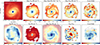 |
Fig. 1. Maps of observed and derived properties of NGC 4321. Top: Convolved and re-gridded SDSS r band, logarithms of stellar mass surface density (Σstar), SFR surface density (ΣSFR), dust mass surface density (Σdust), as well as SED-fitting-derived attenuation in the V band (AV, SED), from left to right. Bottom: Surface density of atomic gas mass (ΣHI), surface density of molecular gas mass (ΣH2), logarithm of the total gas mass surface density (Σgas), dust-to-gas ratio and attenuation in the V band as derived by the BD (AV, BD), from left to right. All maps are at a resolution of 18″. Grey points correspond to pixels that are rejected because they do not have a sufficient number of data points in the FIR regime (see Sect. 2.1.1) or because they are unreliable (see Sect. 2.3 for more details). The ΣHI and ΣH2 maps extend up to their corresponding 3σ limit. In the ΣHI, ΣH2, and AV, BD maps pixels that correspond to the areas that are excluded by the SED-fitting analysis are plotted with smaller dots. In the log10Σgas map, pixels excluded by the SED-fitting analysis and having both H I and CO detection are depicted by smaller squares, while pixels with only H I and not CO are plotted with dots. In the dust-to-gas ratio maps, we limit the colour-coding to the 5th–95th percentile range for illustrative purposes. Contours are taken from the log10Σdust [M⊙ pc−2] maps with a lowest contour at –1.5 and linear spacing with the highest at 0. |
To exclude unreliable estimates of the properties, we used a criterion that is based on the comparison of the best-model value (best) and the likelihood-weighted mean value (bayes) estimated by CIGALE, for each pixel. This has been also adopted in other recent studies (e.g. Buat et al. 2021; Mountrichas et al. 2022; Koutoulidis et al. 2022; Chakraborty et al. 2025). Specifically, we consider in our analysis only pixels where  , for the SED-fitting-derived properties. The bayes value weights all models allowed by the parameter grid, with the best-fit model having the heaviest weight (Boquien et al. 2019). The weight is based on the likelihood, e−χ2/2, associated with each model. A large difference between the two values (i.e. best, bayes) indicates that the fitting did not achieve a reliable estimation of the corresponding parameter. From this criterion, only 24 pixels (1%) were rejected from NGC 0628, 58 pixels (2.7%) from NGC 3351, 13 pixels (1.5%) from NGC 3627, 3 pixels (0.6%) from NGC 4254 and 57 pixels (3.5%) were rejected from NGC 4321.
As is described in Sect. 2.1.1, we discarded the SPIRE 350 μm and 500 μm bands in order to conduct the analysis at higher spatial resolution. However, the choice has minimal consequence on the estimation of the dust luminosity and mass, as we found by performing three independent SED-fitting analyses for one of our targets, NGC 0628. Each time, we used different spectral coverage (i.e. up to 500 μm, up to 350 μm, and up to 250 μm) and resolution (i.e. 36″, 25″, and 18″, respectively) and created the radial profiles of Σdust using bin-widths equal to the resolution of each case. For all cases, we retrieved the same radial profile with the data lying within the uncertainties. We observed a mild overestimation of Σdust when we omitted the 500 μm band, or both 500 μm and 350 μm bands, at a maximum of less than a factor of two, towards the very central part of the galaxy. In a recent study, Chastenet et al. (2024) also shows that the trends and parameter values are well reproduced without considering the two longer wavelength SPIRE bands.
A suite of maps of several parameters for NGC 4321 are shown in Fig. 1, as an example. In the top left panel, we show the convolved and re-gridded SDSS r band for a visual inspection of the morphological structure of the galaxy. The rest panels in the top row show maps of SED-fitting-derived properties (log10Σstar, log10ΣSFR, log10Σdust, AV, SED, from left to right). The bottom panels consist of maps of ΣHI, ΣH2, log10Σgas, Σdust/Σgas and AV, BD, from left to right. The corresponding maps of all galaxies in our sample can be found in Appendix A.
2.4. Data analysis: Geometries and statistical methods
When comparing dust and gas surface densities, we considered face-on values, applying inclination corrections to each galaxy, under the assumption that the ISM is distributed in a thin disc. Attenuations may or may not be inclination-dependent according to the geometrical distribution of the medium providing the attenuation in the case of the AV, BD, or to how dust is distributed with respect to the stellar component if we refer to the attenuated stellar light. For the attenuation inferred by the BD, in the molecular phase for example, inclination corrections are less meaningful because molecular clouds have nearly spherical geometry. Consequently, in plotting the attenuation versus dust surface densities we refer to line of sight values (denoted by the LOS suffix) whether we consider dust mixed with the stars or distributed in a shell around star-forming regions (as also done by Boquien et al. 2013; Kreckel et al. 2013). For completeness, we briefly discuss the correlation coefficients for face-on values as well.
To estimate the scaling relations, we performed fitting through Bayesian inference using the Python UltraNest package (Buchner 2021). UltraNest derives posterior probability distributions and the Bayesian evidence with the nested sampling Monte Carlo algorithm MLFriends (Buchner 2016, 2019). This method provides a robust estimate of the scaling relations between two quantities incorporating the uncertainties of both quantities directly into the fitting process, leading to more reliable estimations of the fitted parameters (i.e. slope and intercept) and their uncertainties. For each correlation we also provide the corresponding statistical coefficients that indicate its significance, i.e. Pearson’s (ρP) and Spearman’s (ρS) coefficients.
3. Results and discussion
The availability of a wide range of multiwavelength data for our galaxies allows us to examine the relation of dust in emission (Σdust) with atomic gas traced by H I (ΣHI), molecular gas traced by CO(2-1) (ΣH2) and the total gas (Σgas), as well as the correlation of optical attenuation derived from the BD (AV, BD) and the stellar light attenuation inferred by SED fitting (AV, SED), with Σgas and Σdust. Based on the AV–Σdust relation, we investigate the dust spatial distribution using also predictions from simple radiative transfer models. Moreover, we compare AV, BD to AV, SED. The correlations among these physical properties are explored in a resolved scale (346 pc, on average; see the pixel size of each galaxy in Table 1).
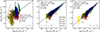 |
Fig. 2. Resolved scaling relations of dust mass surface density with the atomic (left panel), molecular (middle panel) and total gas (right panel) surface density. Each galaxy is represented by a different colour. The median uncertainties for each galaxy are shown in the lower right or lower left corner of the panels. The solid lines are the best linear fits to the full sample, while the shaded grey area indicates the fit uncertainty. The slope, intercept, and scatter of each fit are also given along with the correlation coefficients. In the right panel open circles show pixels where only H I is detected. |
The necessity of using only high-S/N pixels for the derivation of the physical properties through the SED-fitting analysis, limits our study to the main part of the star-forming disc. Moreover, in the discussed correlations that include the AV, BD, we are slightly more limited to the inner part of the disc observed by MUSE. Thus, all the following correlations discussed here do not refer to the outskirts of the galaxies where the ISM is mostly atomic.
3.1. Dust mass surface densities as gas tracers
We examine here which gas phase establishes the best correlation with dust. In Fig. 2 we present the relations between the dust and the gas mass surface densities for galaxies in our sample. More specifically, in the left panel we show the log10Σdust–log10ΣHI relation, in the middle panel the relation between log10Σdust and log10ΣH2, while the correlation of the log10Σdust with the total gas, log10Σgas, is displayed in the right panel.
Although on average galaxies with higher Σdust have also higher ΣHI, the left panel of Fig. 2 shows that these two quantities have a moderate correlation (ρP = 0.55; ρS = 0.53 in the log-log plane) because inside each galaxy Σdust is not often dependent on ΣHI. The average fitted slope is 0.63 ± 0.01 and a significant scatter of 0.25 ± 0.002 is present. An exception is NGC 3627 for which a moderate correlation is found on a resolved scale of 330 pc (ρP = 0.67; ρS = 0.66; slope: 0.94 ± 0.04, scatter: 0.11).
The middle panel of Fig. 2 shows instead that log10Σdust strongly correlates with log10ΣH2 having ρP = 0.91 and ρS = 0.90. The slope of the linear correlation is 0.67 ± 0.004 with a scatter of only 0.09 ± 0.001. The correlation holds also for individual galaxies for which slopes are similar to the global one. An increase in the scatter in the low ΣH2 regime, is a consequence of higher Σdust variations in galaxy’s outskirts and in addition here the use of a constant αCO might not be totally appropriate (see discussion in Appendix B). The sublinear slope between log10Σdust and log10ΣH2 simply states that dust distributions have shallower radial gradients than molecular gas distributions. Assuming that gas and dust can be described by radially exponential discs, it is straightforward to show that the correlation between Σdust and ΣH2 is the inverse of their scale-length ratios. From the slope of the linear fit in the log10Σdust–log10ΣH2 relation, the dust scale-length is thus ∼1.5 times larger (on average) than the molecular gas scale-length. This is compatible with other results in the literature: for instance, Casasola et al. (2017) fit radial exponential profiles to ΣH2 and Σdust and find that, for their sample, the radial scale-length of the dust disc is on average about twice that of the molecular gas disc. We remind here that we have assumed constant values for the CO-to-H2 conversion factors. If instead there are radial variations in αCO (and/or R21), the gradient of the molecular gas might be different from that inferred from the CO distribution. Several studies have found that αCO increases radially (see e.g. Bolatto et al. 2013; Chiang et al. 2024, and Appendix B). A radially increasing αCO would give a flatter radial profile of ΣH2, closer to the Σdust gradient (in this case the slope of the Σdust and ΣH2 correlation increases). For instance, using one of the radial dependent αCO recipes suggested by Chiang et al. (2024), we found that the average slope of the correlation increases, from 0.67 to 0.77 (i.e. the dust scalelength is 1.3× that of molecular gas); however, there is no significant improvement in the correlation strength or in the scatter (see Fig. B.2).
A similar correlation, but with a steeper slope (0.76 ± 0.005), is found between log10Σdust and log10Σgas, as shown in the right panel of Fig. 2. Here ρP = 0.89, ρS = 0.89, and a scatter of 0.12 ± 0.001 are found, larger than for the log10Σdust–log10ΣH2 relation. The correlation parameters remain unchanged if we omit pixels where only atomic gas is detected (open circles). The strength of the correlation between log10Σdust and log10Σgas (Fig. 2, right panel), is almost the same as that with the molecular gas only. This reflects the fact that the gas in the regions examined has a large contribution by the molecular phase. The steeper slope of the correlation is due to the increased contribution of atomic gas at large galactocentric distances. As for the relationship with the molecular gas only, the log10Σdust–log10Σgas correlation seems to depend marginally on the properties of the sampled galaxies. This is in agreement with the findings of Abdurro’uf et al. (2022) that find no significant galaxy-by-galaxy variations in Σdust–ΣH2 and Σdust–Σgas relations. By estimating the best-fit parameters for each galaxy individually, we notice that only the Virgo galaxies (NGC 4254, NGC 4321) have a steeper correlation (slope: 1.04 ± 0.01, 0.84 ± 0.01, respectively) than the mean slope. These findings hold also when we adopt a radially dependent αCO.
3.2. Molecular gas shielding layers and the dust-to-gas ratio
In the left panel of Fig. 2 we notice that every galaxy has a narrow range of ΣHI; these vary only by a factor 2–3 across the disc extent we are examining, with the mean value for each galaxy that changes by about 0.8 dex across the sample. What drives the changes of the mean H I column density from one galaxy to another? One possibility is that variations in the mean ΣHI from galaxy to galaxy are related to molecular shielding. Variations in the shielding H I surface densities might be connected to variations in the dissociating radiation field, of volume gas densities or of the dust-to-gas mass ratio (DGR = Σdust/Σgas). For the DGR we expect ΣHI to increase as the DGR decreases. The average DGRs found in the sampled regions are 0.0033 ± 0.0005, 0.0041 ± 0.001, 0.0048 ± 0.0010, 0.0054 ± 0.0013 and 0.0069 ± 0.0020, for NGC 4254, NGC 0628, NGC 4321, NGC 3627 and NGC 3351, respectively. NGC 4254 is the richest galaxy in gas content and it shows the lowest DGR. Because of this low DGR, the galaxy needs the largest ΣHI of the sample to shield the molecular phase. On the contrary, NGC 3351 has a low gas content and the highest DGR of our sample. Molecules in this case are shielded using a much lower H I column density than for NGC 4254.
The increase in the mean Σdust within the ΣHI range for each galaxy might indicate an increase in Σgas, i.e. an increase in the molecular fraction. To verify this in Fig. 3 we plot the log10Σdust as a function of log10ΣHI, colour coded with atomic gas fraction (fHI = MHI/Mgas) in the top panel and with log10Σstar in the bottom panel. For each galaxy fHI decreases going towards regions with higher dust, indicating an increase in the total gas column density, with the gas becoming more molecular. The bottom panel of Fig. 3 underlines in fact that regions with higher Σdust are places where also Σstar is higher, i.e. the gas layer has higher densities being more compressed by the local stellar gravity, and the formation of molecules is enhanced.
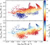 |
Fig. 3. Dust mass surface density as a function of atomic gas mass surface density, colour-coded with atomic gas mass fraction (top panel) and stellar mass surface density (bottom panel) for the whole sample. In both panels, crosses refer to pixels where only H I gas is detected. |
We finally examine in Fig. 4 how the molecular gas fraction (fH2 = MH2/Mgas) varies as a function of the DGR for each galaxy. We find that Sc galaxies (NGC 0628, NGC 4254) have a marginal positive trend with higher fH2 where the DGR is higher, while Sb galaxies hosting a bar (NGC 3351, NGC 3627) have a negative trend on average. A peculiar case is NGC 4321 (SABb) where a transition is observed with pixels having fH2 ≲ 0.8 (outer disc) exhibiting no correlation (or a positive correlation for fH2 ≲ 0.6), while pixels with higher fH2 (central area) having a negative correlation with the DGR. By visually inspecting the DGR map in Fig. 1 we notice the low values in the central area and the rather inhomogeneous distribution in the rest of the disc. The scatter is generally large as in NGC 3351. Here, mainly the central pixels show some correlation with the DGR.
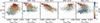 |
Fig. 4. Molecular gas mass fraction as a function dust-to-gas mass ratio, for each galaxy in the sample. The data points are colour coded as a function of galactocentric radius in units of R25. Uncertainties are plotted by grey error bars. |
Our findings might indicate a morphological evolution between Sc and Sb galaxies, possibly related to the presence of a bar. The bar might drag material (dust and gas) towards the centre of the galaxies; during this process, a significant part of the dust can be destroyed by the intense stellar radiation field in that area. This might explain why the DGR remains constant or decreases, while the molecular gas fraction can still increase towards the centre. This is apparent also in the DGR maps (see the corresponding maps in Fig. 1 and Appendix A), where all barred galaxies exhibit a dust-poor centre. Another possibility is that central regions have a lower αCO or a higher R21, as we discuss in detail in Appendix B. For the rest of the discs, given the relatively flat metallicity gradients estimated by Brazzini et al. (2024), with central metallicities of the order of solar, we do not expect strong variations in αCO. Although αCO and R21 variations might give a somewhat different relation between fH2 and the DGR, our analysis in Appendix B confirm the trends shown in Fig. 4.
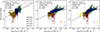 |
Fig. 5. Attenuation on the V band, derived from the BD, as a function of the line-of-sight surface density of the atomic (left panel), molecular (middle panel) and total gas (right panel) mass. Each galaxy is represented by a different colour. The median uncertainties for each galaxy are shown in the top or the lower right corner of the panels. The solid lines are the best linear fits to the full sample, while a shaded area indicates the fit uncertainty. The slope, intercept, and scatter of each fit are also given along with the correlation coefficients. |
3.3. The relations between AV, BD and gas mass surface densities
Here we examine the relation between the V-band attenuation as derived by the BD, AV, BD, with cold gas in the ISM. Our results are shown in Fig. 5, where log10AV, BD is plotted against log10ΣHI (left panel), log10ΣH2 (middle panel) and log10Σgas (right panel). The relations have similar scatter and flatter slopes (indicated in each panel) than those found between Σdust and Σgas. Similarly to what we find for the log10Σdust–log10ΣHI relation, in the left panel of Fig. 5 we see that galaxies which have higher ΣHI have also on average higher AV, BD, but locally, in each galaxy, there is no correlation. The global correlation is moderate (ρP = 0.60; ρS = 0.69).
For log10AV, BD–log10ΣH2 relation, the positive correlation is clear both for individual galaxies and globally for the whole sample. The correlation is moderate if we rely on the correlation coefficients ρP = 0.62, but the value of the Spearman coefficient ρS = 0.78 indicates a stronger correlation of AV, BD with the molecular gas surface density than with the atomic gas. The log10AV, BD has a similar correlation with the log10Σgas than with the log10ΣH2 (ρP = 0.66; ρS = 0.82).
If we correct to face-on values both AV, BD and gas surface densities, the above correlations weaken, the slopes are flatter and the scatter increases. As mentioned in Section 2.4, corrections to face-on values are linked to the geometrical distribution of physical quantities which are not known a priori for the dust providing the attenuation. The stronger correlations we find for line-of-sight values compared to face-on values suggest that the geometric distribution of the absorbing medium is close to spherical. In this case also the attenuation linked to the atomic gas might be driven by HI envelopes around the star formation regimes rather than by the whole atomic gas disc layer. The correlations found between face-on cold gas mass surface densities and AV, BD are also weaker than between the same gas surface densities and Σdust, and underline that only part of the gas and dust mix, present in a galaxy, is responsible for the attenuation of stellar light.
We note that the fitting properties in the log10AV, BD–log10Σgas relations do not change if we exclude pixels detected only in H I (open symbols). To ensure a robust estimation of the correlation, Barrera-Ballesteros et al. (2020) omit cases exhibiting AV[mag] < 0.2 thus excluding regions where CO emission likely drops rapidly due to the photo-dissociation of the CO molecules (van Dishoeck & Black 1988). The exclusion of such pixels does not affect our findings concerning the estimated fitting parameters. In addition, motivated by the fact that we trace slightly different physical scales for galaxies in our sample, we examined the variation in the scatter with respect to the pixel width, but we find no trend. We underline that when we use a radially dependent αCO conversion as suggested by the Chiang et al. (2024) recipe, there is a marginal increase in the strength of the corresponding correlations, but the scatter remains similar (see Fig. B.2).
For NGC 3627 we find the highest AV, BD values among all the regions studied in our sample (confirmed also by the AV, SED). Having this galaxy the highest inclination of all galaxies examined in this paper (i = 67.5°) this finding is consistent with what Concas & Popesso (2019) have also found, namely higher BDs in more inclined galaxies. However, some caution is needed for NGC 3627 because the high AV values are found mainly in the western arm, where an extended polarised radio ridge is, likely caused by ram-pressure compression (Weżgowiec et al. 2012). Ram pressure compression is able to increase locally gas and dust column densities, with a consequent increase in AV (see e.g. Abramson et al. 2011). Nonetheless, excluding NGC 3627 we find similar correlation coefficients for the line-of-sight log10AV, BD–log10ΣH2 relation (ρP = 0.62; ρS = 0.76) and again stronger correlation between log10AV, BD and log10Σgas (ρP = 0.66; ρS = 0.82), as well as slopes and scatters similar to the ones found for the full sample.
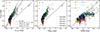 |
Fig. 6. Correlation between the V-band attenuation derived by BD and SED fitting (total, old, and young stars, in the left, middle, and right panels, respectively). Each galaxy is represented by a different colour. A solid line stands for the one-to-one relation. Left panel: AV, BD versus the total attenuation estimated by CIGALE (AV, SED). Points with ΣSFR [ |

3.4. Comparison of AV, BD and AV, SED
A visual inspection of the AV maps displayed in Fig. 1 and Appendix A shows that the attenuations computed via BD and SED fitting have a similar pattern across the discs, although AV, BD is systematically higher than the AV, SED. This is also shown in the left panel of Fig. 6, where the AV derived from the two independent methods are compared. If we focus on the star-forming regions with ![Mathematical equation: $ \Sigma_{\mathrm{SFR}}\,[\mathrm{M}_{\odot}\,\mathrm{Gyr}^{-1}\,\mathrm{pc}^{-2}]\, > \,100 $](/articles/aa/full_html/2025/10/aa55133-25/aa55133-25-eq7.gif) (white data points) the dispersion is reduced. By performing a linear best-fitting analysis on the star-forming regions we find that
(white data points) the dispersion is reduced. By performing a linear best-fitting analysis on the star-forming regions we find that

The slope of our best-fitted linear relation, shown with a dashed line, is slightly higher than the value found for the relation between emission line and stellar continuum AV by Calzetti et al. (2000) (dash-dotted line, slope 0.44) and Kreckel et al. (2013) (dotted line, slope 0.47). We underline that this result is sensitive to the selected attenuation law (i.e. the k(Hα), and k(Hβ) values used in Eq. (3)). In principle, the attenuation law found for each pixel by our SED-fitting analysis, under the assumption of a modified power-law starburst attenuation curve (see Sect. 2.3), might result in a different conversion factor between FHα/FHβ and AV, BD. Nevertheless, we found that, when averaging over all pixels, the factor is very close to that adopted by Kreckel et al. (2013) and thus we use a uniform conversion factor.
The selected SFH and attenuation modules used in our SED-fitting analysis allow us to estimate separately the attenuation on the emission of the old and the young stars. In Fig. 6 middle and right panels, we compare AV, BD with the attenuation on the old (AV, SEDold) and young stars (AV, SEDyoung), respectively. We find that the total attenuation estimated by CIGALE is dominated by AV, SEDold, which is expected, since the bulk of the total stellar content in spiral galaxies is dominated by old stars (see e.g. Nersesian et al. 2019; Paspaliaris et al. 2023). The AV, SEDyoung though, despite the larger uncertainties, is in a quite good agreement with the AV, BD, with the bulk of the data points following the one-to-one relation and 88.6% of them lying within 0.5 dex (dashed grey lines). This indicates that CIGALE is able to estimate the attenuation in star-forming regions on resolved scales, using broadband photometric data only (see also the comparison of the BD-inferred attenuation and SED-fitting-derived attenuation of the birth clouds, in global scales, by Kouroumpatzakis et al. 2021). In a future study, it would be interesting to investigate if the scatter and the uncertainties might decrease by enriching the relative free parameters in the SED fitting with more values and/or by including also narrowband photometric data (e.g. Hα maps) that are available for all the galaxies in our sample. A plateau found at AV, BD ∼ 1.3 mag, might be attributed to the fact that AV, BD and AV, SEDyoung trace different environments with different optical depths at high attenuation values (see also Sect. 3.5 where, at high attenuations, AV, SEDyoung is more closely connected with a dust screen configuration than the AV, BD).
3.5. The correlation of dust in absorption and dust in emission
A visual comparison of the spatial distribution of Σdust, AV, BD and AV, SED across galaxies’ discs can be done using the maps of Fig. 1 and Appendix A, where contours of Σdust are overplotted in all three maps. The pixel-by-pixel relation for each galaxy is shown in Fig. 7 using the AV, BD (left panel), the AV, SEDold (middle panel) and the AV, SEDyoung (right panel). The number of data points is smaller in the first panel because of the restricted extent of MUSE data, compared to the CIGALE SED-fitted area. We observe an increasing trend of Σdust with AV, BD and AV, SEDyoung, rather than AV, SEDold that increases milder as a function of Σdust. This suggests that nebular lines and young stars are more sensitive tracers of the dust mass surface density in our sample. Our finding is in agreement with the results of Muñoz-Mateos et al. (2009) who used the total IR-to-UV ratio, tracing intermediate age stars, to measure the attenuation, and Spitzer imaging to estimate the radial dust properties of nearby galaxies. We also find our results in agreement with those of Kreckel et al. (2013) whose method of analysis is more similar to that adopted in the current study.
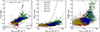 |
Fig. 7. Relation of line-of-sight dust mass surface density with V-band attenuation derived by the BD (left panel), attenuation of the old stars by the SED fitting (middle panel) and attenuation of the young stars also derived by CIGALE (right panel). Uncertainties in both axes are shown in grey. The dust mass surface density estimated under the assumption of a foreground screen dust model is plotted with a solid line. The dotted and dash-dotted curves show the results of the slab and sandwich models, respectively: those in the left panel are for the AV, BD–Σdust relation, those in the central and right panel for AV–Σdust. The best fit of Kreckel et al. (2013) is plotted with a dashed line in the left panel. |
The quantity AV is proportional to the dust surface density only when dust is distributed in a ‘screen’ in front of the sources. Σdust can be directly converted into AV after assuming a DGR (see Eq. (4) in Kreckel et al. 2013). This foreground screen model is shown in Fig. 7, where we use the DGR of the THEMIS model, equal to 0.0074. For the same surface density, lower extinctions can be obtained if dust and stars are distributed in the same layer (the ‘slab’ model; Disney et al. 1989; Calzetti et al. 1994); and even lower if the dust layer is internal to the stellar one (the ‘sandwich’ model; Disney et al. 1989), as emerges from radiative transfer analyses of edge-on galaxies (Xilouris et al. 1999; Bianchi 2007; De Geyter et al. 2013). Results from the slab and sandwich models are shown in Fig. 7. Rather than the analytical solution for a non-scattering medium (Disney et al. 1989) or approximations to include scattering (Calzetti et al. 1994; Kreckel et al. 2013; Boquien et al. 2013) we made a full radiative transfer calculation using the TRADING code (Bianchi 2008), assuming that the thickness of the dust layer is the same (for the slab) or half (for the sandwich) that of stars, and adopting the average properties of the THEMIS model (see Appendix C for details). AV, BD for the slab and sandwich models, derived using Eq. (3), are shown by the dotted and dash-dotted lines of Fig. 7 (left panel), respectively. It is worth noting that AV, BD is not a direct measure of AV and in particular the two quantities diverge for high dust column densities (optical depths). We plot AV for our models in the central and right panel of Fig. 7. The difference is due to the fact that Eq. (3) is formally correct only when the effective attenuations driving the difference between the observed and intrinsic FHα/FHβ follow the same attenuation law, described by the k(Hα) and k(Hβ) values used in the formula. Instead, constant values are used in Eq. (3), while the true attenuation laws change with dust column density because of radiative transfer effects. This is true not only for the models shown in the figure, but also for simpler cases with no scattering (see Appendix C). However, for the surface density range shared by most pixels, AV and AV, BD have similar trends and can be considered as lower limits to the V-band attenuation for our pixels. We also derived attenuations for an exponential model with parameters similar to those derived by fits of edge-on galaxies, but found little differences with the sandwich model (not shown here).
The left panel of Fig. 7 shows that AV, BD is close to the screen model for low Σdust pixels, while it lies between the screen and the slab at higher surface densities. This suggests that the dust that obscures the emitters in the star-forming areas are distributed in a mixed dust and emitting material, as well as a foreground screen dust component. Kreckel et al. (2013) reached similar conclusions, though their best fit to the AV, BD − Σdust correlation (dashed line) tend to be shifted towards higher surface densities; beside differences in the sample and analysis, this could be in part due to different dust emission templates used to derive Σdust (they use those of Draine et al. 2007, which results in dust masses larger by about 50% with respect to those derived using THEMIS; see Nersesian et al. 2019). Our findings are also in accordance with a recent study, in global scales, using GAMA data (i.e. BD and Σdust), by Farley et al. (2025). In that paper it is found that in the case of low dust content, the foreground screen and the mixed geometry (described as ‘distributed’ in their study) both fall in the low BD region, as neither is able to provide enough attenuation to explain the high BD measurements. Furthermore, they report two distinct cases in which, for high dust content, the dust in the screen model is optically thick and prevents emission lines from escaping, leading to a lack of measurements in that regime. In the case of the mixed geometry, lines originating from stars deeply embedded in dust clouds escape less (i.e. are more attenuated) than the ones in the outer regions, allowing for low BD measurements despite the high Σdust in these regions.
As was also shown in the previous section, AV, SEDyoung (right panel of Fig. 7) follows a trend similar to that of AV, BD. Despite the large uncertainties, the attenuation estimated for young stars is consistent with that estimated from the BD. Instead, AV, SEDold more closely follows the models in which stars and dust are mixed (middle panel; slab and sandwich are very close for low column densities), suggesting that the radiation from the old stars is being obscured mainly by the diffuse star-dust geometry of a galactic disc. AV, SEDold also shows that the attenuation does not tend to zero at the lowest column densities, but is biased towards a non-null value. Boquien et al. (2013) noted a similar trend, with non-null attenuation at the lowest gas surface densities, and imputed it to the fact that attenuation is a luminosity-weighted quantity while surface densities are mass-weighted means over the finite extent of a resolution element. It is unclear whether this consideration applies also for our case, given the fact that the Σdust is derived from SED fits to FIR luminosity, unless the biasing due to luminosity weighting acts in different ways on the determination of AV, SEDold and Σdust. Investigating this issue would require a multi-wavelength modelling of a galaxy and the fitting of its SED at different resolutions, which is beyond the scope of the present study.
However, correlations between Σdust and AV, SED derived by the SED fitting should be interpreted with some caution. The two properties are estimated by the same SED-fitting run and under the assumption of energy balance. Although, despite they are expected to be coupled, they are not tightly constrained by each other alone. For instance, a certain IR luminosity can be produced by different amounts of dust mass, under different heating conditions, which are not tightly constrained by the UV–optical data used to fit the attenuation curve. Alternatively, higher Umin (i.e. higher dust temperature) can reduce the need for a high dust mass to explain the IR flux, while still producing a similar attenuation. Indeed, despite the caveat on energy balance our findings regarding the correlations between AV, SEDold, AV, SEDyoung and Σdust are in accordance with the picture derived by the RT models.
4. Summary and conclusions
We have investigated the relation between the dust mass surface density (Σdust), the gas mass surface density (ΣHI, ΣH2, Σgas), and the optical attenuation (AV, BD, AV, SED), throughout the disc of a sample of five nearby spiral galaxies, down to sub-kiloparsec scales. Our main results are summarised as follows:
-
In the regions sampled in this study, which have molecular-fraction fH2 ≳ 0.3, we find that Σdust and AV, BD are better at tracing the molecular and total gas content rather than the atomic gas. The correlations of Σdust with ΣH2 or with Σgas have the strongest significance and hold for individual galaxies as well as for the whole sample.
-
The scaling relations are marginally dependent on galaxy properties. The mean dust-to-gas mass ratio varies across our sample with each galaxy showing local enhancements. Molecular fractions increase as Σdust and Σstar increase.
-
The atomic gas mass surface density for each galaxy is in a restricted range that varies from galaxy to galaxy and is related to the column density that the gas needs to shield the molecular phase. Galaxies with a higher dust-to-gas mass ratio need a lower column density of H I to provide the shielding, with local variations related to the Σstar.
-
The AV, BD and the AV, SEDyoung that we estimated through SED fitting are in very good agreement, with 88.6% of our data points differing by less than 0.5 dex. AV, SEDyoung inferred by CIGALE could serve as a tracer of the attenuation in larger samples, where IFU observations might be more expensive and time-consuming.
-
We estimate the ratio of the AV, BD over the total stellar AV, SED, for star-forming regions, to be equal to 0.59 ± 0.05, slightly larger than the one found in previous studies.
-
Both AV, BD and AV, SEDyoung are affected by a combination of a screen dust component and a mixture of dust and emitting material. On the contrary, AV, SEDold as a function of the Σdust follows the models where sources and dust are mixed (either the slab or the sandwich model).
Data availability
The maps of the derived properties that were used for the main results (see Figs. 2, 4, 5, 6, 7) are available at the CDS via https://cdsarc.cds.unistra.fr/viz-bin/cat/J/A+A/702/A264
Acknowledgments
We are grateful to the anonymous referee for a constructive report that improved the quality of the manuscript. We would like to thank Adam Leroy and Francesco Belfiore for productive discussions on this project and on the use of PHANGS-MUSE data. We acknowledge financial support from: PRIN MIUR 2017 – 20173ML3WW_001; INAF mainstream 2018 program “Gas-DustPedia: A definitive view of the ISM in the Local Universe”; INAF-Mini Grant 2024 program “Dust emission and optical extinction as gas tracers in star forming galaxies”. DustPedia is a collaborative focused research project supported by the European Union under the Seventh Framework Programme (2007–2013) call (proposal no. 606824). The participating institutions are: Cardif University, UK; National Observatory of Athens, Greece; Ghent University, Belgium; Université Paris-Sud, France; National Institute for Astrophysics, Italy and CEA (Paris), France. This work made use of THINGS, ‘The HI Nearby Galaxy Survey’ (Walter et al. 2008) and HERACLES, ‘The HERA CO-Line Extragalactic Survey’ (Leroy et al. 2009). This research made use of Astropy: a community-developed core Python package and an ecosystem of tools and resources for astronomy (Astropy Collaboration 2013, 2018, 2022, http://www.astropy.org); matplotlib, a Python library for publication quality graphics (Hunter 2007); NumPy (Harris et al. 2020); SciPy (Virtanen et al. 2020); TOPCAT, an interactive graphical viewer and editor for tabular data (Taylor 2005); Photutils, an Astropy package for detection and photometry of astronomical sources (Bradley et al. 2024).
References
- Abdo, A. A., Ackermann, M., Ajello, M., et al. 2010, ApJ, 710, 133 [Google Scholar]
- Abdurro’uf, Lin, Y. T., Hirashita, H., et al. 2022, ApJ, 935, 98 [CrossRef] [Google Scholar]
- Abramson, A., Kenney, J. D. P., Crowl, H. H., et al. 2011, AJ, 141, 164 [Google Scholar]
- Amorín, R., Muñoz-Tuñón, C., Aguerri, J. A. L., & Planesas, P. 2016, A&A, 588, A23 [NASA ADS] [CrossRef] [EDP Sciences] [Google Scholar]
- Anand, G. S., Lee, J. C., Van Dyk, S. D., et al. 2021, MNRAS, 501, 3621 [Google Scholar]
- Aniano, G., Draine, B. T., Gordon, K. D., & Sandstrom, K. 2011, PASP, 123, 1218 [Google Scholar]
- Astropy Collaboration (Robitaille, T. P., et al.) 2013, A&A, 558, A33 [NASA ADS] [CrossRef] [EDP Sciences] [Google Scholar]
- Astropy Collaboration (Price-Whelan, A. M., et al.) 2018, AJ, 156, 123 [Google Scholar]
- Astropy Collaboration (Price-Whelan, A. M., et al.) 2022, ApJ, 935, 167 [NASA ADS] [CrossRef] [Google Scholar]
- Barrera-Ballesteros, J. K., Utomo, D., Bolatto, A. D., et al. 2020, MNRAS, 492, 2651 [NASA ADS] [CrossRef] [Google Scholar]
- Battisti, A., Shivaei, I., Park, H. J., et al. 2025, PASA, 42, e022 [Google Scholar]
- Bianchi, S. 2007, A&A, 471, 765 [NASA ADS] [CrossRef] [EDP Sciences] [Google Scholar]
- Bianchi, S. 2008, A&A, 490, 461 [NASA ADS] [CrossRef] [EDP Sciences] [Google Scholar]
- Bolatto, A. D., Wolfire, M., & Leroy, A. K. 2013, ARA&A, 51, 207 [CrossRef] [Google Scholar]
- Boquien, M., Buat, V., Boselli, A., et al. 2012, A&A, 539, A145 [NASA ADS] [CrossRef] [EDP Sciences] [Google Scholar]
- Boquien, M., Boselli, A., Buat, V., et al. 2013, A&A, 554, A14 [NASA ADS] [CrossRef] [EDP Sciences] [Google Scholar]
- Boquien, M., Kennicutt, R., Calzetti, D., et al. 2016, A&A, 591, A6 [NASA ADS] [CrossRef] [EDP Sciences] [Google Scholar]
- Boquien, M., Burgarella, D., Roehlly, Y., et al. 2019, A&A, 622, A103 [NASA ADS] [CrossRef] [EDP Sciences] [Google Scholar]
- Bradley, L., Sipőcz, B., Robitaille, T., et al. 2024, https://doi.org/10.5281/zenodo.13989456 [Google Scholar]
- Brazzini, M., Belfiore, F., Ginolfi, M., et al. 2024, A&A, 691, A173 [NASA ADS] [CrossRef] [EDP Sciences] [Google Scholar]
- Brinchmann, J., Charlot, S., Kauffmann, G., et al. 2013, MNRAS, 432, 2112 [CrossRef] [Google Scholar]
- Bruzual, G., & Charlot, S. 2003, MNRAS, 344, 1000 [NASA ADS] [CrossRef] [Google Scholar]
- Buat, V., Noll, S., Burgarella, D., et al. 2012, A&A, 545, A141 [NASA ADS] [CrossRef] [EDP Sciences] [Google Scholar]
- Buat, V., Mountrichas, G., Yang, G., et al. 2021, A&A, 654, A93 [NASA ADS] [CrossRef] [EDP Sciences] [Google Scholar]
- Buchner, J. 2016, Stat. Comput., 26, 383 [Google Scholar]
- Buchner, J. 2019, PASP, 131, 108005 [Google Scholar]
- Buchner, J. 2021, J. Open Source Softw., 6, 3001 [CrossRef] [Google Scholar]
- Calzetti, D., Kinney, A. L., & Storchi-Bergmann, T. 1994, ApJ, 429, 582 [Google Scholar]
- Calzetti, D., Armus, L., Bohlin, R. C., et al. 2000, ApJ, 533, 682 [NASA ADS] [CrossRef] [Google Scholar]
- Cardelli, J. A., Clayton, G. C., & Mathis, J. S. 1989, ApJ, 345, 245 [Google Scholar]
- Casasola, V., Cassarà, L. P., Bianchi, S., et al. 2017, A&A, 605, A18 [NASA ADS] [CrossRef] [EDP Sciences] [Google Scholar]
- Casasola, V., Bianchi, S., De Vis, P., et al. 2020, A&A, 633, A100 [NASA ADS] [CrossRef] [EDP Sciences] [Google Scholar]
- Casasola, V., Bianchi, S., Magrini, L., et al. 2022, A&A, 668, A130 [NASA ADS] [CrossRef] [EDP Sciences] [Google Scholar]
- Catinella, B., Haynes, M. P., Giovanelli, R., Gardner, J. P., & Connolly, A. J. 2008, ApJ, 685, L13 [Google Scholar]
- Chakraborty, A., Kundu, M., Chatterjee, S., et al. 2025, A&A, 694, A140 [NASA ADS] [CrossRef] [EDP Sciences] [Google Scholar]
- Chastenet, J., De Looze, I., Relaño, M., et al. 2024, A&A, 690, A348 [NASA ADS] [CrossRef] [EDP Sciences] [Google Scholar]
- Chiang, I.-D., Sandstrom, K. M., Chastenet, J., et al. 2024, ApJ, 964, 18 [NASA ADS] [CrossRef] [Google Scholar]
- Chung, A., van Gorkom, J. H., Kenney, J. D. P., Crowl, H., & Vollmer, B. 2009, AJ, 138, 1741 [Google Scholar]
- Ciesla, L., Charmandaris, V., Georgakakis, A., et al. 2015, A&A, 576, A10 [NASA ADS] [CrossRef] [EDP Sciences] [Google Scholar]
- Clark, C. J. R., Verstocken, S., Bianchi, S., et al. 2018, A&A, 609, A37 [NASA ADS] [CrossRef] [EDP Sciences] [Google Scholar]
- Concas, A., & Popesso, P. 2019, MNRAS, 486, L91 [Google Scholar]
- Corbelli, E., Bianchi, S., Cortese, L., et al. 2012, A&A, 542, A32 [NASA ADS] [CrossRef] [EDP Sciences] [Google Scholar]
- Cormier, D., Bigiel, F., Jiménez-Donaire, M. J., et al. 2018, MNRAS, 475, 3909 [NASA ADS] [CrossRef] [Google Scholar]
- Cutri, R. M., Skrutskie, M. F., van Dyk, S., et al. 2003, VizieR On-line Data Catalog: II/246 [Google Scholar]
- Dame, T. M., Hartmann, D., & Thaddeus, P. 2001, ApJ, 547, 792 [Google Scholar]
- Davies, J. I., Nersesian, A., Baes, M., et al. 2019, A&A, 626, A63 [NASA ADS] [CrossRef] [EDP Sciences] [Google Scholar]
- De Geyter, G., Baes, M., Fritz, J., & Camps, P. 2013, A&A, 550, A74 [NASA ADS] [CrossRef] [EDP Sciences] [Google Scholar]
- den Brok, J. S., Chatzigiannakis, D., Bigiel, F., et al. 2021, MNRAS, 504, 3221 [NASA ADS] [CrossRef] [Google Scholar]
- Disney, M., Davies, J., & Phillipps, S. 1989, MNRAS, 239, 939 [NASA ADS] [CrossRef] [Google Scholar]
- Draine, B. T., Dale, D. A., Bendo, G., et al. 2007, ApJ, 663, 866 [NASA ADS] [CrossRef] [Google Scholar]
- Eisenstein, D. J., Weinberg, D. H., Agol, E., et al. 2011, AJ, 142, 72 [Google Scholar]
- Emsellem, E., Schinnerer, E., Santoro, F., et al. 2022, A&A, 659, A191 [NASA ADS] [CrossRef] [EDP Sciences] [Google Scholar]
- Farley, B., Ahmed, U. T., Hopkins, A., et al. 2025, PASA, 42 [Google Scholar]
- Fazio, G. G., Hora, J. L., Allen, L. E., et al. 2004, ApJS, 154, 10 [Google Scholar]
- Fitzpatrick, E. L. 1999, PASP, 111, 63 [Google Scholar]
- Foyle, K., Wilson, C. D., Mentuch, E., et al. 2012, MNRAS, 421, 2917 [Google Scholar]
- Gil de Paz, A., Boissier, S., Madore, B. F., et al. 2007, ApJS, 173, 185 [Google Scholar]
- Griffin, M. J., Abergel, A., Abreu, A., et al. 2010, A&A, 518, L3 [EDP Sciences] [Google Scholar]
- Grossi, M., Corbelli, E., Bizzocchi, L., et al. 2016, A&A, 590, A27 [NASA ADS] [CrossRef] [EDP Sciences] [Google Scholar]
- Harris, C. R., Millman, K. J., van der Walt, S. J., et al. 2020, Nature, 585, 357 [NASA ADS] [CrossRef] [Google Scholar]
- Hensley, B. S., & Draine, B. T. 2021, ApJ, 906, 73 [NASA ADS] [CrossRef] [Google Scholar]
- Hughes, T. M., Baes, M., Fritz, J., et al. 2014, A&A, 565, A4 [NASA ADS] [CrossRef] [EDP Sciences] [Google Scholar]
- Hummer, D. G., & Storey, P. J. 1987, MNRAS, 224, 801 [NASA ADS] [CrossRef] [Google Scholar]
- Hunter, J. D. 2007, Comput. Sci. Eng., 9, 90 [NASA ADS] [CrossRef] [Google Scholar]
- Israel, F. P. 2020, A&A, 635, A131 [NASA ADS] [CrossRef] [EDP Sciences] [Google Scholar]
- Jones, A. P., Köhler, M., Ysard, N., Bocchio, M., & Verstraete, L. 2017, A&A, 602, A46 [NASA ADS] [CrossRef] [EDP Sciences] [Google Scholar]
- Kouroumpatzakis, K., Zezas, A., Maragkoudakis, A., et al. 2021, MNRAS, 506, 3079 [NASA ADS] [CrossRef] [Google Scholar]
- Koutoulidis, L., Mountrichas, G., Georgantopoulos, I., Pouliasis, E., & Plionis, M. 2022, A&A, 658, A35 [NASA ADS] [CrossRef] [EDP Sciences] [Google Scholar]
- Kovačić, I., Barnes, A. T., Bigiel, F., et al. 2025, A&A, 694, A87 [NASA ADS] [CrossRef] [EDP Sciences] [Google Scholar]
- Kreckel, K., Groves, B., Schinnerer, E., et al. 2013, ApJ, 771, 62 [NASA ADS] [CrossRef] [Google Scholar]
- Leitherer, C., Li, I. H., Calzetti, D., & Heckman, T. M. 2002, ApJS, 140, 303 [NASA ADS] [CrossRef] [Google Scholar]
- Leroy, A. K., Walter, F., Brinks, E., et al. 2008, AJ, 136, 2782 [Google Scholar]
- Leroy, A. K., Walter, F., Bigiel, F., et al. 2009, AJ, 137, 4670 [Google Scholar]
- Leroy, A. K., Bigiel, F., de Blok, W. J. G., et al. 2012, AJ, 144, 3 [Google Scholar]
- Leroy, A. K., Schinnerer, E., Hughes, A., et al. 2021, ApJS, 257, 43 [NASA ADS] [CrossRef] [Google Scholar]
- Leroy, A. K., Rosolowsky, E., Usero, A., et al. 2022, ApJ, 927, 149 [NASA ADS] [CrossRef] [Google Scholar]
- Martin, D. C., Fanson, J., Schiminovich, D., et al. 2005, ApJ, 619, L1 [Google Scholar]
- Momcheva, I. G., Lee, J. C., Ly, C., et al. 2013, AJ, 145, 47 [NASA ADS] [CrossRef] [Google Scholar]
- Morrissey, P., Conrow, T., Barlow, T. A., et al. 2007, ApJS, 173, 682 [Google Scholar]
- Mountrichas, G., Masoura, V. A., Xilouris, E. M., et al. 2022, A&A, 661, A108 [NASA ADS] [CrossRef] [EDP Sciences] [Google Scholar]
- Muñoz-Mateos, J. C., Gil de Paz, A., Boissier, S., et al. 2009, ApJ, 701, 1965 [CrossRef] [Google Scholar]
- Nersesian, A., Xilouris, E. M., Bianchi, S., et al. 2019, A&A, 624, A80 [NASA ADS] [CrossRef] [EDP Sciences] [Google Scholar]
- Noll, S., Burgarella, D., Giovannoli, E., et al. 2009, A&A, 507, 1793 [NASA ADS] [CrossRef] [EDP Sciences] [Google Scholar]
- Orellana, G., Nagar, N. M., Elbaz, D., et al. 2017, A&A, 602, A68 [NASA ADS] [CrossRef] [EDP Sciences] [Google Scholar]
- Osterbrock, D. E., & Ferland, G. J. 2006, Astrophysics of Gaseous Nebulae and Active Galactic Nuclei (Sausalito, CA: University Science Books) [Google Scholar]
- Paspaliaris, E. D., Xilouris, E. M., Nersesian, A., et al. 2021, A&A, 649, A137 [NASA ADS] [CrossRef] [EDP Sciences] [Google Scholar]
- Paspaliaris, E. D., Xilouris, E. M., Nersesian, A., et al. 2023, A&A, 669, A11 [NASA ADS] [CrossRef] [EDP Sciences] [Google Scholar]
- Pilbratt, G. L., Riedinger, J. R., Passvogel, T., et al. 2010, A&A, 518, L1 [NASA ADS] [CrossRef] [EDP Sciences] [Google Scholar]
- Piotrowska, J. M., Bluck, A. F. L., Maiolino, R., Concas, A., & Peng, Y. 2020, MNRAS, 492, L6 [Google Scholar]
- Poglitsch, A., Waelkens, C., Geis, N., et al. 2010, A&A, 518, L2 [NASA ADS] [CrossRef] [EDP Sciences] [Google Scholar]
- Rieke, G. H., Young, E. T., Engelbracht, C. W., et al. 2004, ApJS, 154, 25 [Google Scholar]
- Roehlly, Y., Burgarella, D., Buat, V., et al. 2014, in Astronomical Data Analysis Software and Systems XXIII, eds. N. Manset, & P. Forshay, Astronomical Society of the Pacific Conference Series, 485, 347 [NASA ADS] [Google Scholar]
- Salpeter, E. E. 1955, ApJ, 121, 161 [Google Scholar]
- Salvestrini, F., Bianchi, S., & Corbelli, E. 2025, A&A, 699, A346 [NASA ADS] [CrossRef] [EDP Sciences] [Google Scholar]
- Sandstrom, K. M., Leroy, A. K., Walter, F., et al. 2013, ApJ, 777, 5 [Google Scholar]
- Schlafly, E. F., & Finkbeiner, D. P. 2011, ApJ, 737, 103 [Google Scholar]
- Schruba, A., Leroy, A. K., Walter, F., et al. 2011, AJ, 142, 37 [NASA ADS] [CrossRef] [Google Scholar]
- Shetty, R., Glover, S. C., Dullemond, C. P., et al. 2011, MNRAS, 415, 3253 [NASA ADS] [CrossRef] [Google Scholar]
- Skrutskie, M. F., Cutri, R. M., Stiening, R., et al. 2006, AJ, 131, 1163 [NASA ADS] [CrossRef] [Google Scholar]
- Strong, A. W., & Mattox, J. R. 1996, A&A, 308, L21 [NASA ADS] [Google Scholar]
- Taylor, M. B. 2005, in Astronomical Data Analysis Software and Systems XIV, eds. P. Shopbell, M. Britton, & R. Ebert, Astronomical Society of the Pacific Conference Series, 347, 29 [Google Scholar]
- Teng, Y.-H., Sandstrom, K. M., Sun, J., et al. 2022, ApJ, 925, 72 [NASA ADS] [CrossRef] [Google Scholar]
- Tody, D. 1986, in Instrumentation in Astronomy VI, ed. D. L. Crawford, Society of Photo-Optical Instrumentation Engineers (SPIE) Conference Series, 627, 733 [NASA ADS] [CrossRef] [Google Scholar]
- Tody, D. 1993, in Astronomical Data Analysis Software and Systems II, eds. R. J. Hanisch, R. J. V. Brissenden, & J. Barnes, Astronomical Society of the Pacific Conference Series, 52, 173 [Google Scholar]
- van Dishoeck, E. F., & Black, J. H. 1988, ApJ, 334, 771 [Google Scholar]
- Verheijen, M., Deshev, B., van Gorkom, J., et al. 2010, arXiv e-prints [arXiv:1009.0279] [Google Scholar]
- Virtanen, P., Gommers, R., Oliphant, T. E., et al. 2020, Nat. Methods, 17, 261 [Google Scholar]
- Walter, F., Brinks, E., de Blok, W. J. G., et al. 2008, AJ, 136, 2563 [Google Scholar]
- Werner, M. W., Roellig, T. L., Low, F. J., et al. 2004, ApJS, 154, 1 [NASA ADS] [CrossRef] [Google Scholar]
- Weżgowiec, M., Soida, M., & Bomans, D. J. 2012, A&A, 544, A113 [NASA ADS] [CrossRef] [EDP Sciences] [Google Scholar]
- Wong, T., & Blitz, L. 2002, ApJ, 569, 157 [CrossRef] [Google Scholar]
- Wright, E. L., Eisenhardt, P. R. M., Mainzer, A. K., et al. 2010, AJ, 140, 1868 [Google Scholar]
- Xilouris, E. M., Byun, Y. I., Kylafis, N. D., Paleologou, E. V., & Papamastorakis, J. 1999, A&A, 344, 868 [NASA ADS] [Google Scholar]
- Yajima, Y., Sorai, K., Miyamoto, Y., et al. 2021, PASJ, 73, 257 [NASA ADS] [CrossRef] [Google Scholar]
- York, D. G., Adelman, J., Anderson, J. E., Jr., et al. 2000, AJ, 120, 1579 [NASA ADS] [CrossRef] [Google Scholar]
Appendix A: Maps of galaxies’ properties
In this Appendix we show maps of the resolved properties of galaxies in our sample, at a resolution of 18".
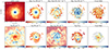 |
Fig. A.1. Maps of observed and derived properties of NGC 0628. Top: Convolved and re-gridded SDSS r band, log10Σstar, log10ΣSFR, log10Σdust, as well as SED-fitting-derived V-band attenuation (AV, SED), from left to right. Bottom: ΣHI, ΣH2, log10Σgas, DGR and V-band attenuation derived by the BD (AV, BD), from left to right. Grey points correspond to pixels that are rejected (see Sec. 2.1.1, 2.3 for more details). The ΣHI and ΣH2 maps extend up to their corresponding 3σ limit. For ΣHI, ΣH2 and AV, BD maps pixels that correspond to areas excluded by the SED-fitting analysis are plotted with smaller dots. In log10Σgas map, pixels excluded by the SED-fitting analysis and having both H I and CO detection are depicted by smaller squares, while pixels with only H I and not CO are plotted with dots. Contours plotted in some map are from log10Σdust [M⊙ pc−2] maps with a lowest contour at -1.3 and linear spacing with the highest at -0.9. Dots in each map indicate areas excluded fro the SED fitting routine. |
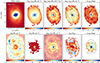 |
Fig. A.2. Same as Fig. A.1, but for NGC 3351. Contours are taken from the log10Σdust [M⊙ pc−2] maps with a lowest contour at -1.5 and linear spacing with the highest at 0. |
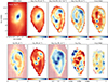 |
Fig. A.3. Same as Fig. A.1, but for NGC 3627. Contours are taken from the log10Σdust [M⊙ pc−2] maps with a lowest contour at -1.5 and linear spacing with the highest at -0.7. |
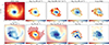 |
Fig. A.4. Same as Fig. A.1, but for NGC 4254. Contours are taken from the log10Σdust [M⊙ pc−2] maps with a lowest contour at -1.1 and linear spacing with the highest at -0.5. |
 |
Fig. A.5. Same as Fig. A.1, but for NGC 4321. Contours are taken from the log10Σdust [M⊙ pc−2] maps with a lowest contour at -1.5 and linear spacing with the highest at 0. |
Appendix B: CO-to-H2 conversion factor αCO and CO(2-1)-to-CO(1-0) line ratio R21
In this appendix, we discuss our assumptions to infer the molecular gas surface density from 12CO J = 2-1 line maps and possible dependencies of our results from these assumptions. As stated in the main paper we used a MW-disc CO-to-H2 conversion factor aCO= 4.4 M⊙ pc−2 (K km s−1)−1 (Bolatto et al. 2013) and an intrinsic line ratio R21=ICO(2 − 1)/ICO(1 − 0) = 0.7 (e.g. Leroy et al. 2009; Schruba et al. 2011). Although these values have been widely used by previous studies of the ISM in nearby galaxies (e.g. Casasola et al. 2017), variations in these two parameters are possible due to variations in local ISM conditions in clouds, such as metallicity, temperature, mass surface density, velocity dispersion, and optical thickness. The metallicity dependencies of αCO have been studied by many authors (e.g. Amorín et al. 2016) but for our sample metallicities are very close to solar (Brazzini et al. 2024) and we do not expect significant deviations from the assumed value across the bright discs we investigate. Other studies have found αCO to deviate from the typical MW in galaxy’s central regions (e.g. Israel 2020; Teng et al. 2022).
Dedicated surveys for accurate determination of αCO often include galaxies of our sample, such as the CO-isotopologue investigation by Cormier et al. (2018) or the dust based studies by Sandstrom et al. (2013) and Chiang et al. (2024). The usage of CO isotopologues as tracers of molecular mass primarily traces dense gas, leading to underestimation of the total molecular mass, given the presence of diffuse molecular gas in the ISM. Sandstrom et al. (2013) used the dust as gas tracer and the gas-to-dust ratio to infer αCO in kiloparsec-scale regions. They found an average αCO radial profile that is generally flat, with a depression towards the centre, particularly evident for NGC 3351, NGC 3627 and NGC 4321 (R < 0.1R25). In the same area, the αCO was found significantly increased in NGC 4254. They provided average ICO-weighted values for each galaxy and as optimal average αCO for the whole sample, 3.1 M⊙ pc−2 (K km s−1)−1. Chiang et al. (2024) using a similar method, studies the variation in αCO as a function of several physical quantities, and find negative anti-correlations with SFR, radiation field intensity, CO intensity and galactocentric distance.
Galaxies in our sample have also been targets for R21 investigations. Although these are also discussed by Sandstrom et al. (2013), we use the data of more recent and dedicated surveys, which give resulting values more consistent between each other and with our assumed ratio (den Brok et al. 2021; Yajima et al. 2021; Leroy et al. 2022). These works find R21 in the range of 0.45 – 0.83 as average values across the disc of galaxies in our sample. The mean of the three values (two only for NGC 3351) reported for each galaxy by den Brok et al. (2021), Yajima et al. (2021) and by Leroy et al. (2022) are 0.56, 0.67, 0.50, 0.69, 0.72 for NGC 0628, NGC 3351, NGC 3627, NGC 4254, and NGC 4321, respectively. These are within 30% of our assumed R21 ratio, with NGC 4254 and NGC 4321 fully consistent with our assumed R21 ratio. There are no significant radial variations measured for the region of interest in galaxies of our sample. Only for NGC 3627 and NGC 4321 the ALMA observations analysed by den Brok et al. (2021) show a positive radial gradient or a factor 1.5 enhancement in the centre, respectively. These radial variations are not however confirmed by other observations such as HERACLES (IRAM-30m) data. We notice that for NGC 3627 and NGC 4321 results of different analyses give somewhat different mean values. Because of these discrepancies we have considered a uniform R21 = 0.7 ratio in the present study.
With the aim to verify if our results are significantly affected by variations in αCO and R21 with respect to the assumed values, in Fig. B.1 we plot the fH2 as a function of the DGR for four different cases. In the top row, we assume the typical αCO = 4.4 M⊙ pc−2 (K km s−1)−1 as in the rest of the paper (same as Fig. 4 but with a common x-axis range for all galaxies); in the second row, the average αCO values found by Sandstrom et al. (2013) for each galaxy with a constant R21 has been used; in the third row, we set αCO = 4.4 M⊙ pc−2 (K km s−1)−1 and use R21 = 0.56, 0.67, 0.50, 0.69, 0.72 for NGC 0628, NGC 3351, NGC 3627, NGC 4254, and NGC 4321, respectively. In addition, for NGC 3351, NGC 3627, and NGC 4321 we use a 1.5 enhancement factor in R21 and a factor 2 decrease in αCO for the central region; finally, in the bottom row, we use the correlation found by Chiang et al. (2024) between αCO(2 − 1) and galactocentric distance (with no need to correct for R21). The pixels that lie in the R < 0.15 R25 areas are plotted with open symbols.
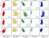 |
Fig. B.1. Molecular gas mass fraction as a function dust-to-gas mass ratio, for each galaxy in the sample. The molecular gas is estimated assuming a constant MW αCO = 4.4 M⊙ pc−2 (K km s−1)−1 (Bolatto et al. 2013 and R21 = 0.7 (top panels), a radially constant αCO which varies from galaxy to galaxy as found by Sandstrom et al. (2013) (middle-top panels), a constant αCO = 4.4 M⊙ pc−2 (K km s−1)−1 throughout the galaxies except in the central areas, and a radially constant R21 value varying from galaxy to galaxy (den Brok et al. 2021; Yajima et al. 2021; Leroy et al. 2022, middle-bottom panels), and a radially varying αCO(2 − 1) as found by Chiang et al. (2024, bottom panels). The αCO and R21 values used for each panel are shown in the lower right corners. Pixels within the inner 0.15 R25 area are plotted with open symbols. Uncertainties are shown with grey error bars. |
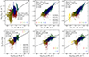 |
Fig. B.2. Top panels, same as in Fig. 2 and bottom panels same as in Fig. 5, but with using the Chiang et al. (2024) prescription for a radially varying αCO (see text for details.) |
The main conclusion of our investigation in this Appendix is that by changing our assumptions on R21 and on αCO we recover similar DGR trends across the galaxies and from one galaxy to another. Although molecular fractions change, these always increase with the DGR for NGC 0628 and NGC 4254. If we exclude the central area, for which the CO-to-H2 conversion factor can be lower than what has been shown in Fig. B.1, NGC 3351 and NGC 4321 have no correlation between the molecular fraction and the DGR where the molecular phase dominates, while NGC 3627 shows a decreasing DGR as the molecular fraction increases. NGC 4321 shows a decrease in the dust abundance on the outskirts, under all assumptions apart from the case of the radially dependent αCO by Chiang et al. (2024). In this case the main part of the disc shows a mild positive correlation, with some deviation for outskirts and centre. In an increasing order we list the average DGRs found in the sampled regions: 0.0033 ± 0.0005, 0.0041 ± 0.001, 0.0048 ± 0.0010, 0.0054 ± 0.0013 and 0.0069 ± 0.0020, for NGC 4254, NGC 0628, NGC 4321, NGC 3627, and NGC 3351, respectively, using the standard values as in the main paper. These values increase by decreasing αCO but the sequence is unchanged; also when using the Chiang et al. 2024 αCO prescription, with the only exception of NGC 4321 which in this case has a DGR equal to 0.0039 ± 0.001 and is second in increasing order, instead of being third (see Sec. 3.2).
We have also estimated the best-fit parameters and the correlation coefficients for the log10Σdust–log10ΣH2 and log10Σdust–log10Σgas relations for various αCO and R21 and we do not find significant differences. For instance, if we use the Chiang et al. (2024) prescription where αCO changes with galactocentric distance, the correlations of log10Σdust with log10ΣH2 and log10Σgas, as well as log10AV, BD with log10ΣH2 and log10Σgas, have similar slopes, scatter and correlation significance to those found using a constant αCO (see Fig. B.2). We prefer to use the constant αCO values in the main paper to avoid any possible influence of circular reasoning: in fact the Chiang et al. (2024) prescription is found assuming that the total gas surface density is traced by the dust surface density given a constant gas-to-metal ratio. Thus we would study the correlation of Σdust with a quantity that has been derived using Σdust (though assuming a different dust model than ours, as in Chiang et al. 2024). Nevertheless, similar correlations (not shown here) are found also using the Bolatto et al. (2013) formula that accounts for a decrease in αCO in denser regions (see their Eq. 31). This is recovered using several methodologies and not only using dust as a proxy of gas. In any case, the αCO variations mostly affect central areas, which are only a small portion of the discs we investigate, and do not affect our main conclusions.
Appendix C: Attenuations for simple geometries
For a homogeneously mixed thin layer of dust and sources, of optical depth τλ perpendicular to the layer, the radiative transfer solution can be derived analytically in the absence of scattering: it is the slab model (Disney et al. 1989) and the corresponding attenuation can be written as
 (C.1)
(C.1)
where, for simplicity, we consider only the line of sight perpendicular to the layer (face-on view). For τλ → 0, Eq. C.1 can be written using series expansion as
 (C.2)
(C.2)
Instead, for τ → ∞, it is
 (C.3)
(C.3)
Using these limits, τλ = k(λ)τV with k(λ) the (V-band normalised) extinction law, and Eq. 3, rewritten as
 (C.4)
(C.4)
we can easily find that AV, BD tends to AV for low optical depths, and to the constant value 2.5log10(k(Hβ)/k(Hα))/(k(Hβ) − k(Hα)) at high optical depths. This is shown in Fig. C.1, where we plot AV, BD vs AV for a slab using the extinction law of the THEMIS dust model (k(Hα) = 0.81, k(Hβ) = 1.14).
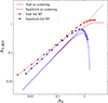 |
Fig. C.1. AV, BD vs AV for the models discussed in the text. The dotted line shows the 1-to-1 relation. |
For the sandwich model, it is
 (C.5)
(C.5)
where hs is the thickness of the source layer and hd ≤ hs is that of a dust layer internal to the source one and sharing the same mid-plane: the solution is the combination of a slab model, of the dust-free portion of sources on the side opposite to the viewer attenuated by the dust screen, and of the unattenuated symmetric portion on the side of the viewer (the first, second and third terms of the logarithm in Eq. C.5, respectively; the sandwich is equivalent to the slab for hd = hs). As for the slab, AV, BD is the same as AV in the optically thin limit. Instead, it goes to zero as 1/τV at high AV. The case for hd = hs/2 is shown in Fig. C.1.
For the slab and sandwich models we also made full radiative transfer calculation including scattering: we used the TRADING code (Bianchi 2008), assuming hd = hs/2 and albedos from the THEMIS model [ω(Hα) = 0.56, ω(Hβ) = 0.52]; and strong forward scattering, with an asymmetry parameter characteristic for MW dust, g = 0.7, at both wavelengths (Hensley & Draine 2021). We run 19 models with face-on optical depth τV between 0.1 and 20.
Results from radiative transfer calculations are also shown in Fig. C.1. The trends are qualitatively similar to the no-scattering cases, but with differences between AV, BD and AV also in the optically thin limit. The full radiative transfer results for the slab and sandwich models are also discussed in Sect. 3.5 and plotted in Fig. 7.
All Tables
Summary of the multi-wavelength observational data used in the current analysis with their references.
All Figures
|
Fig. 1. Maps of observed and derived properties of NGC 4321. Top: Convolved and re-gridded SDSS r band, logarithms of stellar mass surface density (Σstar), SFR surface density (ΣSFR), dust mass surface density (Σdust), as well as SED-fitting-derived attenuation in the V band (AV, SED), from left to right. Bottom: Surface density of atomic gas mass (ΣHI), surface density of molecular gas mass (ΣH2), logarithm of the total gas mass surface density (Σgas), dust-to-gas ratio and attenuation in the V band as derived by the BD (AV, BD), from left to right. All maps are at a resolution of 18″. Grey points correspond to pixels that are rejected because they do not have a sufficient number of data points in the FIR regime (see Sect. 2.1.1) or because they are unreliable (see Sect. 2.3 for more details). The ΣHI and ΣH2 maps extend up to their corresponding 3σ limit. In the ΣHI, ΣH2, and AV, BD maps pixels that correspond to the areas that are excluded by the SED-fitting analysis are plotted with smaller dots. In the log10Σgas map, pixels excluded by the SED-fitting analysis and having both H I and CO detection are depicted by smaller squares, while pixels with only H I and not CO are plotted with dots. In the dust-to-gas ratio maps, we limit the colour-coding to the 5th–95th percentile range for illustrative purposes. Contours are taken from the log10Σdust [M⊙ pc−2] maps with a lowest contour at –1.5 and linear spacing with the highest at 0. |
| In the text | |
|
Fig. 2. Resolved scaling relations of dust mass surface density with the atomic (left panel), molecular (middle panel) and total gas (right panel) surface density. Each galaxy is represented by a different colour. The median uncertainties for each galaxy are shown in the lower right or lower left corner of the panels. The solid lines are the best linear fits to the full sample, while the shaded grey area indicates the fit uncertainty. The slope, intercept, and scatter of each fit are also given along with the correlation coefficients. In the right panel open circles show pixels where only H I is detected. |
| In the text | |
|
Fig. 3. Dust mass surface density as a function of atomic gas mass surface density, colour-coded with atomic gas mass fraction (top panel) and stellar mass surface density (bottom panel) for the whole sample. In both panels, crosses refer to pixels where only H I gas is detected. |
| In the text | |
|
Fig. 4. Molecular gas mass fraction as a function dust-to-gas mass ratio, for each galaxy in the sample. The data points are colour coded as a function of galactocentric radius in units of R25. Uncertainties are plotted by grey error bars. |
| In the text | |
|
Fig. 5. Attenuation on the V band, derived from the BD, as a function of the line-of-sight surface density of the atomic (left panel), molecular (middle panel) and total gas (right panel) mass. Each galaxy is represented by a different colour. The median uncertainties for each galaxy are shown in the top or the lower right corner of the panels. The solid lines are the best linear fits to the full sample, while a shaded area indicates the fit uncertainty. The slope, intercept, and scatter of each fit are also given along with the correlation coefficients. |
| In the text | |
|
Fig. 6. Correlation between the V-band attenuation derived by BD and SED fitting (total, old, and young stars, in the left, middle, and right panels, respectively). Each galaxy is represented by a different colour. A solid line stands for the one-to-one relation. Left panel: AV, BD versus the total attenuation estimated by CIGALE (AV, SED). Points with ΣSFR [ |
| In the text | |
|
Fig. 7. Relation of line-of-sight dust mass surface density with V-band attenuation derived by the BD (left panel), attenuation of the old stars by the SED fitting (middle panel) and attenuation of the young stars also derived by CIGALE (right panel). Uncertainties in both axes are shown in grey. The dust mass surface density estimated under the assumption of a foreground screen dust model is plotted with a solid line. The dotted and dash-dotted curves show the results of the slab and sandwich models, respectively: those in the left panel are for the AV, BD–Σdust relation, those in the central and right panel for AV–Σdust. The best fit of Kreckel et al. (2013) is plotted with a dashed line in the left panel. |
| In the text | |
|
Fig. A.1. Maps of observed and derived properties of NGC 0628. Top: Convolved and re-gridded SDSS r band, log10Σstar, log10ΣSFR, log10Σdust, as well as SED-fitting-derived V-band attenuation (AV, SED), from left to right. Bottom: ΣHI, ΣH2, log10Σgas, DGR and V-band attenuation derived by the BD (AV, BD), from left to right. Grey points correspond to pixels that are rejected (see Sec. 2.1.1, 2.3 for more details). The ΣHI and ΣH2 maps extend up to their corresponding 3σ limit. For ΣHI, ΣH2 and AV, BD maps pixels that correspond to areas excluded by the SED-fitting analysis are plotted with smaller dots. In log10Σgas map, pixels excluded by the SED-fitting analysis and having both H I and CO detection are depicted by smaller squares, while pixels with only H I and not CO are plotted with dots. Contours plotted in some map are from log10Σdust [M⊙ pc−2] maps with a lowest contour at -1.3 and linear spacing with the highest at -0.9. Dots in each map indicate areas excluded fro the SED fitting routine. |
| In the text | |
|
Fig. A.2. Same as Fig. A.1, but for NGC 3351. Contours are taken from the log10Σdust [M⊙ pc−2] maps with a lowest contour at -1.5 and linear spacing with the highest at 0. |
| In the text | |
|
Fig. A.3. Same as Fig. A.1, but for NGC 3627. Contours are taken from the log10Σdust [M⊙ pc−2] maps with a lowest contour at -1.5 and linear spacing with the highest at -0.7. |
| In the text | |
|
Fig. A.4. Same as Fig. A.1, but for NGC 4254. Contours are taken from the log10Σdust [M⊙ pc−2] maps with a lowest contour at -1.1 and linear spacing with the highest at -0.5. |
| In the text | |
|
Fig. A.5. Same as Fig. A.1, but for NGC 4321. Contours are taken from the log10Σdust [M⊙ pc−2] maps with a lowest contour at -1.5 and linear spacing with the highest at 0. |
| In the text | |
|
Fig. B.1. Molecular gas mass fraction as a function dust-to-gas mass ratio, for each galaxy in the sample. The molecular gas is estimated assuming a constant MW αCO = 4.4 M⊙ pc−2 (K km s−1)−1 (Bolatto et al. 2013 and R21 = 0.7 (top panels), a radially constant αCO which varies from galaxy to galaxy as found by Sandstrom et al. (2013) (middle-top panels), a constant αCO = 4.4 M⊙ pc−2 (K km s−1)−1 throughout the galaxies except in the central areas, and a radially constant R21 value varying from galaxy to galaxy (den Brok et al. 2021; Yajima et al. 2021; Leroy et al. 2022, middle-bottom panels), and a radially varying αCO(2 − 1) as found by Chiang et al. (2024, bottom panels). The αCO and R21 values used for each panel are shown in the lower right corners. Pixels within the inner 0.15 R25 area are plotted with open symbols. Uncertainties are shown with grey error bars. |
| In the text | |
|
Fig. B.2. Top panels, same as in Fig. 2 and bottom panels same as in Fig. 5, but with using the Chiang et al. (2024) prescription for a radially varying αCO (see text for details.) |
| In the text | |
|
Fig. C.1. AV, BD vs AV for the models discussed in the text. The dotted line shows the 1-to-1 relation. |
| In the text | |
Current usage metrics show cumulative count of Article Views (full-text article views including HTML views, PDF and ePub downloads, according to the available data) and Abstracts Views on Vision4Press platform.
Data correspond to usage on the plateform after 2015. The current usage metrics is available 48-96 hours after online publication and is updated daily on week days.
Initial download of the metrics may take a while.