| Issue |
A&A
Volume 702, October 2025
|
|
|---|---|---|
| Article Number | A196 | |
| Number of page(s) | 7 | |
| Section | Planets, planetary systems, and small bodies | |
| DOI | https://doi.org/10.1051/0004-6361/202555220 | |
| Published online | 17 October 2025 | |
Solar wind energy deposition related to hydrogen energetic neutral atoms in the Martian upper atmosphere observed by MAVEN
1
Key Laboratory of Planetary Science and Frontier Technology, Institute of Geology and Geophysics, Chinese Academy of Sciences,
Beijing
100029,
PR China
2
College of Earth and Planetary Sciences, University of Chinese Academy of Sciences,
Beijing
100049,
PR China
3
Beijing National Observatory of Space Environment, Institute of Geology and Geophysics, Chinese Academy of Sciences,
Beijing
100029,
PR China
4
Heilongjiang Mohe Observatory of Geophysics, Institute of Geology and Geophysics, Chinese Academy of Sciences,
Beijing
100029,
PR China
★ Corresponding author: This email address is being protected from spambots. You need JavaScript enabled to view it.
Received:
19
April
2025
Accepted:
1
September
2025
Abstract
The coupling between the solar wind and the Martian upper atmosphere is an important topic for the Martian space environment. Due to the induced magnetosphere of Mars, solar wind particles are largely prevented from entering the Martian ionosphere. Instead, studies suggest that solar wind protons undergo charge exchange with atmospheric hydrogen atoms to produce hydrogen energetic neutral atoms (H-ENAs) that penetrate the upper atmosphere and deposit energy. The H-ENAs at ionospheric altitudes of Mars are difficult to detect directly. Proton aurorae are thought to be a result of H-ENA deposition. Laboratory experiments have demonstrated that collisions between H-ENAs and Martian atmospheric CO2 produce both H+ and H−. In this study, we present a particular event in which collision-induced H+ and H−, along with the Martian proton aurora, were simultaneously recorded by the Mars Atmosphere and Volatile EvolutioN (MAVEN) spacecraft. H+ and H− propagate in the anti-sunward direction, and their energies gradually dissipate with decreasing altitudes, accompanied by the auroral emission intensity reaching its maximum. Furthermore, the observed H+∕H−flux ratio closely matches laboratory data. The results strongly support H-ENA deposition into the Martian upper atmosphere and the correlation between Martian proton aurorae and ionospheric energetic H+ and H−. This study enhances our understanding of the solar wind interactions with the Martian space environment.
Key words: plasmas / methods: observational / planets and satellites: atmospheres / planets and satellites: aurorae / planets and satellites: individual: Mars
© The Authors 2025
 Open Access article, published by EDP Sciences, under the terms of the Creative Commons Attribution License (https://creativecommons.org/licenses/by/4.0), which permits unrestricted use, distribution, and reproduction in any medium, provided the original work is properly cited.
This article is published in open access under the Subscribe to Open model. This email address is being protected from spambots. You need JavaScript enabled to view it. to support open access publication.
1 Introduction
The interaction between the solar wind and the Martian space environment is crucial for understanding the evolution of the Martian atmosphere. It is widely accepted that solar wind particles cannot penetrate deeply into the Martian ionosphere (Kallio & Barabash 2001; Lundin et al. 2004; Chaufray et al. 2020). Instead, they can interact with neutral hydrogen atoms in the Martian hydrogen corona through charge exchange processes, resulting in the production of hydrogen energetic neutral atoms (H-ENAs) and pickup ions (Kallio et al. 1997, 2006; Kallio & Barabash 2000; Hara et al. 2018). These H-ENAs retain energy characteristics of the upstream solar wind, thereby serving as valuable tracers for studying the solar wind-Martian space environment coupling. H-ENAs are unaffected by electromagnetic fields, allowing them to pass through the Martian bow shock (BS) and the induced magnetic boundary (IMB), and ultimately deposit their energies into the thermosphere through three primary mechanisms: electron stripping, electron attachment, and excitation (Halekas et al. 2015a; Wang et al. 2013; Hughes et al. 2019; Girazian & Halekas 2021; Henderson et al. 2022).
Observational evidence of penetrating H-ENAs at Mars remains scarce. Mars Express (MEX) was the first spacecraft to observe Martian H-ENAs. MEX detected H-ENAs in the magnetosheath (Brinkfeldt et al. 2006), with some of these atoms being reflected near the IMB (Futaana et al. 2006). Additionally, the presence of H-ENAs has been documented in the vicinity of the Martian magnetotail (Gunell et al. 2006). Although MEX carried an instrument that could directly detect ENAs, it operated at altitudes above 270 km. Further observations are needed to investigate how the H-ENAs interact with the Martian upper atmosphere, particularly at lower altitudes (100-200 km), where atmospheric density is significantly higher than that at the MEX orbit. The Mars Atmosphere and Volatile EvolutioN (MAVEN) spacecraft typically operates at an average altitude of 150 km. During “Deep Dip” campaigns, MAVEN descends to altitudes as low as 110-130 km, effectively bridging this observational gap (Jakosky et al. 2015). Between altitudes of 120 and 400 km, H-ENAs collide with the predominant atmospheric particles, i.e., carbon dioxide (CO2) in the Martian atmosphere, leading to the generation of H+ and H− through electron stripping and attachment (Lillis et al. 2008; Shematovich et al. 2011; Diéval et al. 2012). MAVEN detects these H+ and H− particles, which retain energy signatures from the upstream solar wind, allowing inferences to be made about H-ENAs (Halekas et al. 2017; Wang et al. 2018). The spacecraft provides a unique dataset for investigating solar wind energy deposition into the Martian atmosphere.
Approximately 4-15% of upstream solar wind H-ENAs produce H+ (Halekas 2017; Henderson et al. 2021), while only 0.290.78% of upstream solar wind H-ENAs produce H− (Henderson et al. 2024). The relative fluxes of H+ and H− ions are primarily governed by the corresponding collision cross sections of H-ENAs and CO2 molecules. Experimental measurements reveal a 10:1 ratio between the cross sections of electron stripping and attachment for 1 keV hydrogen atoms interacting with CO2 (Lindsay et al. 2005). Thus, the detection of H− is infrequent (Henderson et al. 2024). Halekas et al. (2015a) observed both pervasive H+ beams and infrequent H− beams within the Martian magnetosphere after coronal mass ejection events using MAVEN measurements. Although this simultaneous observation occurred at an altitude of 160 km, no concurrent observations were reported at lower altitudes during the “Deep Dip” campaigns of MAVEN. The fluxes of H+ and H− are directly influenced by the prevailing upstream solar wind conditions and exhibit seasonal variability, with peak fluxes occurring around perihelion (Jones et al. 2022). Furthermore, previous studies reported that the ratio of H− to upstream solar wind proton density varies in response to fluctuations in upstream solar wind conditions, whereas the ratio of H−∕H+ density remains relatively stable (Jones et al. 2022). The scarcity of H− observations has limited studies on their flux ratio.
Besides the fraction of H-ENAs that can undergo ionization, it has also been suggested that enhanced Lyman-alpha (Ly-α) emissions in the Martian upper atmosphere, i.e., proton aurorae, are caused by the energy deposition of H-ENAs (Deighan et al. 2018; Hughes et al. 2019; Ritter et al. 2018). Hughes et al. (2019) demonstrated that the brightness and occurrence rate of the Martian proton aurora peak at low solar zenith angles (SZAs) on the dayside and seasonally near the southern summer solstice, based on MAVEN Ly-α limb observations spanning two Martian years. Other studies indicate that during the disturbed solar wind conditions, solar wind-driven proton auroral brightening is synchronized with increased atmospheric ion loss (He et al. 2023). Three primary mechanisms all contribute to H-ENA energy dissipation in the Martian upper atmosphere. However, their relative contributions across different altitude ranges have not been characterized due to observational constraints.
Further studies on H-ENAs and their energy deposition in the Martian upper atmosphere are essential to better understand the coupling between the solar wind and the Martian space environment. Although theoretically H-ENA deposition into the Martian upper atmosphere can result in observable phenomena through three primary mechanisms, including collision-induced H+ and H− and Martian proton aurorae, no simultaneous observation or co-occurrence of these three phenomena has been reported. Acquiring additional observations is critical for constructing a sequence of processes for solar wind energy deposition via H-ENAs in the Martian upper atmosphere. In this study, we report a comprehensive event in which MAVEN detected interactions between H-ENAs and the atmosphere below 200 km via three primary mechanisms. Energy losses of H+ and H− accompanied by enhanced proton aurorae were recorded by MAVEN. The results support H-ENA deposition into the Martian upper atmosphere caused by the solar wind-Martian hydrogen corona interaction and three primary energy loss mechanisms of H-ENAs.
2 MAVEN data
The MAVEN spacecraft has been orbiting Mars in an elliptical orbit with a 4.5 h period since September 2014. It carries eight scientific instruments to measure the Martian space environment. MAVEN is capable of conducting comprehensive sampling of the solar wind, the Martian upper atmosphere, and the ionosphere. The Solar Wind Electron Analyzer (SWEA; Mitchell et al. 2016) and the Solar Wind Ion Analyzer (SWIA; Halekas et al. 2015b) are integral components of the MAVEN instrument suite. They are designed primarily to measure the energy, flux, and angular distribution of energetic charged particles in the Martian space environment.
SWIA is designed to measure solar wind ions and can also detect energetic ions within the Martian upper atmosphere, providing information on both the solar wind and its interaction with the Martian atmosphere. SWIA operates over an energy range of 25 eV to 25 keV, with a temporal resolution of 4 seconds. SWIA has a field of view of 360° azimuth × 90° elevation and an angular resolution of 22.5° × 22.5°. Ion directions can be determined from 16 azimuthal bins (A0-A15) and four elevation bins (D0-D3) provided by SWIA. In this study, we used the “onboardsyspec” and “Coarse-3D” data to quantify ion fluxes and directions.
Although it is generally difficult to distinguish H− from ionospheric electrons in ionospheric observations, SWEA measures all negatively charged particles within the energy range of 3 eV to 4.6 keV via “SvySpec” data. This capability enables the identification of energetic H− in the upper atmosphere based on energy spectra and altitude. SWEA has a time resolution of 2 seconds and a field of view of 360° azimuth × 120° elevation. This instrument provides six elevation bins with a 20° angular bin size, similar to its 22.5° azimuthal bin size.
The Supra-Thermal And Thermal Ion Composition (STATIC) instrument is designed to measure supra-thermal and thermal ions in the Martian space environment. It covers an energy range from 0.1 eV to 30 keV and comprises 32 energy bins (McFadden et al. 2015). STATIC has the capability of distinguishing ion composition thanks to its 64 mass bins. We used STATIC observations to identify the ion composition observed by SWIA in the upper atmosphere. The mass fluxes used in this study are primarily based on the “C6” data product.
We also used the Neutral Gas and Ion Mass Spectrometer (NGIMS) to measure the CO2 density of the Martian upper atmosphere (Mahaffy et al. 2015). NGIMS characterizes Mars’ upper atmospheric composition between altitudes of 125500 km. This instrument simultaneously measures densities of reactive and inert neutral gases (including CO2) and ambient ions along the spacecraft track. With its mass spectrometry capabilities, NGIMS complements MAVEN’s suite of instruments studying solar wind interactions with the Martian system.
For proton auroral observations, we employed data from the Imaging UltraViolet Spectrograph (IUVS). This instrument comprises a far-ultraviolet (FUV; 110-190 nm) channel and a mid-ultraviolet (MUV; 180-340 nm) channel (McClintock et al. 2015). It provides 12 limb scans to characterize the composition and structure of the upper atmosphere over a 23-minute period during which MAVEN’s orbital altitude is below 500 km. IUVS FUV limb scans produce altitude-intensity profiles of hydrogen Ly-α emissions at 121.6 nm to identify proton aurorae. In this study, IUVS instrument was employed to detect auroral emissions during the identified H+ and H− events. SWIA, SWEA, and STATIC conduct in situ particle measurements, while IUVS remotely senses auroral emissions, enabling multi-scale analysis. In this study, data from the MAVEN spacecraft were utilized in the Mars Solar Orbital (MSO) coordinates (Vignes et al. 2000). In this coordinate system, the X-axis points from Mars to the Sun, the Y-axis opposes the direction of the orbital motion of Mars, and the Z-axis completes the right-hand coordinate system.
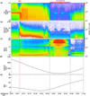 |
Fig. 1 MAVEN in situ observations during 16:00-17:00 UT on 24 April 2018 including (a) the SWIA ion energy spectrum, (b) the SWEA electron energy spectrum, (c) the STATIC mass spectrum, (d) the MAVEN spacecraft altitude, and (e) the SZA at the MAVEN spacecraft position. The vertical dashed red line marks the BS crossing. The vertical dashed purple lines and the horizontal purple bar at the top of Fig. 1 indicate the time intervals during which MAVEN was in the Martian ionosphere. The H+ and H− event is shown by the horizontal red bar at the top of Fig. 1. |
3 Results and discussion
We identify one case study of hydrogen deposition observed by the MAVEN spacecraft on 24 April 2018. Notably, this particular event demonstrates the complete energy deposition process related to penetrating solar wind H-ENAs. Fig. 1 shows the plasma environment near Mars observed by MAVEN between 16:00 and 17:00 UT on 24 April 2018, during which the event was recorded.
During this period, the spacecraft sequentially traversed the solar wind, magnetosheath, and ionosphere (Luhmann et al. 2004). As MAVEN crossed the Martian BS (marked by the vertical dashed red line in Fig. 1), the ion energy spectra (Fig. 1a) exhibited significant broadening, and suprathermal electron fluxes became prominent in the electron spectra (Fig. 1b), due to magnetosheath plasma compression heating. The mass spectra (Fig. 1c) reveal a transition in the dominant ion composition from solar wind protons (~1 amu) to planetary ions (O+ and O2+ corresponding to 16 amu and 32 amu, respectively) (Brain et al. 2010). This indicates that the spacecraft passed through the IMB into the Martian ionosphere. The vertical dashed purple lines mark the observational interval during which MAVEN traversed the ionosphere. These boundaries were determined visually, based on the characteristics described in Wang et al. (2020), Matsunaga et al. (2017), and Trotignon et al. (2006). Figures 1a and 1b show that ions and electrons were colder in the ionosphere than in the magnetosheath. Meanwhile, it is notable that Figures 1a and 1b also show that both SWIA and SWEA simultaneously observed significant flux enhancements of H+ and H− exceeding background levels within the energy range of 500-1000 eV in the ionospheric region. The energy range of these particles (500-1000 eV) corresponds to the expected energy of penetrating H-ENAs (around 1 keV) and is higher than the energies of photoelectrons and Auger electrons (which are typically below 500 eV) (Jones et al. 2022; Mitchell et al. 2000). Halekas et al. (2015a) reported that SWIA detected monoener-getic protons with upstream solar wind velocities in the dayside thermosphere at altitudes below 250 km, which were identified as a result of penetrating H-ENAs. We can identify the ion species related to penetrating H-ENAs from observational data by analyzing their location, energy range, flux, and direction (Halekas et al. 2015a; Henderson et al. 2024). The signature of penetrating protons is observed as an anti-sunward beam at altitudes below 200 km in the Martian atmosphere(Halekas et al. 2017). At ionospheric altitudes, these H-ENAs are converted back into charged particles, primarily H+ and occasionally H−, which have been simultaneously observed by MAVEN (Halekas et al. 2015a). Under quiet space weather conditions, the expected energy range of these reionized protons lies between 540 eV and 1720 eV, corresponding to typical solar wind speeds at Mars of 324-578 km s−1 (Girazian & Halekas 2021). Girazian & Halekas (2021) reported that the typical penetrating proton flux observed by SWIA is on the order of ~104−105 eV∕(eV cm2 s sr), which is consistent with this event. The lack of a corresponding charged population at intermediate altitudes indicates that these protons originate from H-ENAs that travel deep into the atmosphere and are subsequently reionized (Halekas et al. 2015a). Additionally, during this H+ and H− event, the “Coarse-3D” SWIA data show spatially consistent H+ flux enhancements at ~1 keV in sectors aligned with the solar wind, indicating that the observed ions are traveling anti-sunward.
The energies of precipitating H-ENAs originate from the upstream solar wind. Existing observations in the ionospheric region indicate that below 200 km these particles are primarily governed by atmospheric collisional processes (Henderson et al. 2024). Collisional processes with neutral species give rise to two main effects: on the one hand, H-ENA energy is partially released in the form of proton aurora; on the other hand, energies of H+ and H− may be partially transferred to the upper atmosphere. Energies of H+ and H− should decline with decreasing altitude within this deposition framework. Figs. 2a and 2b present the selected H+ and H− energy spectra during the event after removing background fluxes. To identify H+ and H− populations, we applied a combination of methodologies outlined in Girazian & Halekas (2021) and Henderson et al. (2022, 2024). We performed Gaussian fits on each SWIA and SWEA energy spectrum after excluding those affected by negative spacecraft charging and high-energy pickup ion signals, as they are not representative of the penetrating proton population under study. From the Gaussian fits, we derived the expected value (μ) and variance (σ) of the distribution. The core region, which spans energies of μ ± σ, was used to extract the flux associated with the penetrating population in each spectrum. The background corrected core fluxes falling within this energy range are plotted in panels a and b of Fig. 2. Background values were dynamically determined for each time slice of the differential energy flux spectrum by averaging the fluxes in the four highest energy bins (Girazian & Halekas 2021; Henderson et al. 2024). Each computed background was then subtracted from all flux measurements within its respective spectrum. This method was uniformly applied to both H+ and H− populations, as is demonstrated in Fig. 2. In this case, the resulting average background level of H+ is approximately 7.0×10³ eV/(eV cm2 s sr), which is consistent with the reported range of penetrating proton background levels (4.0 × 10³−6.7 × 10³ eV∕(eV cm2 s sr)) between 2015 and 2020 (Girazian & Halekas 2021). Fig. 2 demonstrates that the H+ and H− event spans two orbits: orbit 6938 prior to 16:39:48 UT and orbit 6939 following this time. MAVEN’s altitude is displayed as the dashed red line. Evident trends of declining energy with decreasing altitudes are observed for both H+ and H−. We calculated the weighted average energies (Ē) of H+ and H− at different altitudes from the energy-count distributions, as is illustrated by the black dots in Fig. 2. Assuming the spectra contain n channels (energy bins), the weighted average energy is given by
 (1)
(1)
where Ei is the central energy corresponding to the i-th channel, Ci is the count (weight) of the i-th channel, and  is the total count of the spectrum. The weighted average energies of H+ exhibit a significant decrease with descending altitude. Although some H− energies vary considerably due to poor data quality, the overall trend still reflects the energy decrease to some extent. Fig. 2c shows the CO2 density variation measured by NGIMS during this event period. This event occurred during a “Deep Dip” campaign. It can be seen that the CO2 density increases exponentially with decreasing altitude, accompanied by the declining energy trend in H+ and H− energy spectra. The significantly enhanced neutral density means that H-ENAs encounter intensified collisions so that their energies progressively dissipate, which leads to declining energies of H+ and H− produced by H-ENA collisions with CO2. Halekas (2017) observed that H+ densities decrease at the lowest altitudes due to collisions with neutrals, which scatter the ions and dissipate their energy. At altitudes below 160 km where the CO2 column content exceeds 5×1016 cm−2, the normalized energy fluxes of precipitating H+ begin to decrease sharply (Henderson et al. 2021). Henderson et al. (2024) anticipated similar behavior for H−; however, the H−fluxes did not exhibit a pronounced decline. We observe anticipated features in the altitude-dependent energy decrease. H+ exhibits a stark decline, meanwhile H− shows an overall decrease in energy. When atmospheric CO2 approximately reaches its maximum value at 120-130 km (Mahaffy et al. 2015a; Stone et al. 2018), energetic H+ and H− disappear. This collision-driven energy dissipation supports the interpretation that ionospheric energetic H+ and H− are caused by the downward deposition of H-ENAs.
Figs. 2a and 2b also indicate that the energy fluxes of H+ and H− differ significantly. That is the case if H+ and H− are produced by the collisions between H-ENAs and Martian atmospheric CO2 according to laboratory measurements (Lindsay et al. 2005). Halekas et al. (2015a) also demonstrated that negative ion fractions resulting from electron attachment are an order of magnitude lower than positive fractions. To quantify the flux ratio between H+ and H− populations, we fit Gaussian functions to the differential energy flux spectra of each species at each time slice. From each fit, we extracted the centroid energy and peak flux, which represent the characteristic energy and flux of the particle population. Fig. 3a shows the Gaussian centroid energies and peak fluxes for H+ and H−. This approach avoids ambiguities caused by the different energy bin definitions of SWIA and SWEA. Due to the time resolution discrepancy between SWIA and SWEA, we adopted the SWEA temporal resolution as the baseline. Each 4-second SWIA data point was split into two segments to match the 2-second SWEA resolution. The data were divided into six energy bins, with boundaries indicated by the vertical dashed gray lines in Fig. 3b, based on the density of data points. For each bin, the medians of the H+ and H− peak fluxes were computed as representative values. These medians were then used to calculate the H+/H− flux ratio. The error bars of the H+/H− flux ratio were calculated from the quartile values of the H+ and H− fluxes within each energy bin. The upper bound of the ratio was calculated as the upper quartile of H+ flux divided by the lower quartile of H− flux. Conversely, the lower bound was calculated as the lower quartile of H+ flux divided by the upper quartile of H− flux. In Fig. 3b, gray circles show the median flux ratios plotted at the central energy of each bin; vertical error bars indicate the quartile-based bounds. Laboratory measurements indicate that the ratio is approximately 10 for collisions between 1 keV H-ENAs and CO2 , and tends to decline with decreasing impinging H-ENA energies below 2 keV (Lindsay et al. 2005). As is shown by the dashed gray line in Fig. 3b, the trend of the peak H+/H− flux ratio is basically consistent with laboratory measurements and agrees with the expected energy-dependent collision processes of H-ENAs. The ratio approaches roughly 10 at a centroid energy of ~ 1 keV. We also calculated the H+/H− flux ratio based on the Gaussian-fit peak fluxes for each time slice. The occurrence rate distribution of the calculated flux ratios is shown in Fig. 3c. The occurrence rate shows an abnormal distribution; it has a peak at a lower H+/H− flux ratio of 4.88 and significantly extends toward higher ratio values. This is consistent with the average H+/H− flux ratio of 4.5 reported by Henderson et al. (2024). This distribution pattern is characteristic of a log-normal distribution. The red curve in Fig. 3c shows a log-normal fit to the occurrence rate distribution. A log-normal distribution often arises from the multiplicative interactions of several independent factors (Limpert et al. 2001). In this context, the H+∕H− flux ratio is influenced by multiple factors such as the collision cross section, incident atom energy, and CO2 column density along deposition paths (Lindsay et al. 2005). Notably, the peak flux ratio of 4.88 in Fig. 3c closely matches the average value of 4.5 reported by Henderson et al. (2024). In their study, they compared H+ and H− fluxes as a function of CO2 column density using MAVEN dayside periapsis observations from 2014 to 2023.
Another phenomenon that it has been suggested is related to the H-ENA deposition is the proton aurora on Mars. Ly-α emissions at 121.6 nm can be generated by the H-ENA transition from the excited state (2p) to the ground state (1s), which form proton aurorae (Kallio & Barabash 2001). Hughes et al. (2019) report that proton aurorae occur more frequently at low SZAs on the dayside. Fig. 1e indicates that the SZA of MAVEN was approximately 60° during this H+ and H− event, indicating that the event occurred at a moderate SZA location on the dayside. IUVS limb observations of atmospheric emission intensity were used to investigate Ly-α emission variation during this event, aiming to examine the relationship between the H+ and H− event and proton aurorae. Fig. 4a presents the brightness profiles of Ly-α and other emissions associated with CO2 ionization and dissociation in three adjacent orbits, including orbit 6937 (before the event), orbit 6938 (the event), and orbit 6939 (the event). The profiles of orbit 6937 are typical of Martian UV dayglow (Deighan et al. 2018). The Ly-α emission demonstrates a relatively flat profile due to multiple scatterings during orbit 6937, while other emissions related to CO2 ionization and dissociation display pronounced peaks at altitudes of around 125 km. The Ly-α emission exhibits significant enhancements at lower altitudes in orbits 6938 and 6939, especially in the range of 100-150 km, where brightness peaks form near 125 km (Ritter et al. 2018).
No significant changes are detected among the three orbits in the brightness profiles of other emissions associated with CO2 ionization and dissociation. The characteristics of orbits 6938 and 6939 confirm the presence of proton aurorae. Meanwhile, the observed H+ and H− signals also appear in these two orbits. That is to say, MAVEN simultaneously observed the H+ and H− signals along with the proton aurora. The relationship between the proton aurorae and the H+ and H− event can be further examined by comparing the energy loss process of H+ and H− with the altitudinal distribution of Ly-α emission intensity.
The Ly-α emission can partially reduce H-ENA energy. Below 150 km, the Ly-α emission intensity increases, accompanied by a gradual attenuation of H+ and H− energies (Fig. 2). At altitudes of 120-130 km, proton aurora intensity peaks, and energetic H+ and H−, cannot be detected by MAVEN. The Ly-α emission intensity peak means that there is maximum H-ENA energy loss. The H-ENA energy should attenuate to low levels very quickly with decreasing altitudes below the emission peak due to significantly increased neutral density. As a result, the H+ and H− cannot be produced via collisional ionization between energetic H-ENAs and atmospheric particles below 120 km, indicating that collisional excitation is the dominant energy loss mechanism at this altitude (Kallio & Barabash 2001). Halekas et al. (2015a) observed populations of H+ and H− with solar wind energies in the Martian atmosphere. They speculated that penetrating protons (H+) might be associated with proton aurora. Subsequent observations by Deighan et al. (2018) confirmed this conjecture, revealing that proton aurorae observed by IUVS correlate with increasing penetrating proton fluxes measured by SWIA. Hughes et al. (2025) also observed an expected correlation between the Ly-α emission enhancement and penetrating proton flux. However, they revealed a decrease in the ratio of penetrating proton flux to Ly-α enhancement, indicating a more pronounced Ly-α enhancement compared to the penetrating proton flux. They also demonstrated that amplified Ly-α enhancements are associated with dust storms and extreme solar activity. While previous studies identified a direct correlation between penetrating H+ and proton auroral emissions and anticipated their co-occurrence with H−, we report the first clear observation of all three phenomena occurring simultaneously.
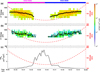 |
Fig. 2 Temporal evolutions of (a) the corresponding H+ energy spectrum, (b) the H− energy spectrum, and (c) CO2 density variation measured by NGIMS during the H-ENA penetration event on 24 April 2018. The altitude of the MAVEN spacecraft is plotted with the dashed red line on the right axis. The weighted average energies obtained from H+ and H− count-energy distributions within 4-second and 2-second time windows are represented by the black dots. The horizontal magenta and blue bars at the top of Fig. 2 represent orbits 6938 and 6939, respectively. |
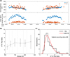 |
Fig. 3 (a) Gaussian-fit centroid energies and peak fluxes of H+ and H− at each time step are shown. H+ and H− data are represented by solid blue and orange points, respectively. (b) The gray circles show the H+/H− flux ratio at the central energy of each bin, and the vertical error bars represent the quartile-based bounds. Vertical dashed gray lines indicate the bin boundaries, while the dashed gray line shows the overall trend of the H+∕H− flux ratio. (c) Percentage distribution of H+∕H− flux ratios. The most frequently occurring ratio is 4.88. The log-normal fit to this distribution is shown by the red curve. |
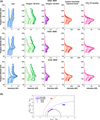 |
Fig. 4 IUVS limb observations for the emission intensity profiles of Ly-α and CO2 ionization and dissociation emissions during orbits 6937, 6938, and 6939. Each panel contains 12 profiles from 12 limb scans indicated by varying color intensities. MAVEN trajectories during the H-ENA penetration event within (b) ( |

4 Summary
The deposition of H-ENAs into the Martian upper atmosphere is thought to play a key role in the solar wind coupling with the Martian space environment. These particles are difficult to detect directly in the lower thermosphere due to H-ENA interactions with the denser atmosphere. Although H-ENA collision-induced H+, H−, and proton aurorae have been proposed to be tracers of H-ENA deposition, there have not been any simultaneous observations of H+, H−, and proton aurorae to support this so far. In this study, we present an event during a “Deep Dip” campaign of MAVEN, in which energetic H+,H−, and enhanced proton aurorae are simultaneously recorded at altitudes below 200 km by multiple instruments on board MAVEN. H+ and H− move antisunward, and their energies decline as the Co2 density increases exponentially when MAVEN approaches periapsis. Accompanied by the decrements of H+ and H− energies, the Ly-α emission intensity is enhanced compared to the background emission level. The energetic H+ and H− disappear at 120-130 km, where the proton aurora intensity reaches a peak value of approximately 9.7 kR. These observational features are well in line with the H-ENA deposition into the upper atmosphere that originates from the solar wind interaction with the Martian hydrogen corona. Moreover, the H+/H− flux ratio shows a decreasing trend with declining energies of H+ and H , and the highest occurring is 4.88. These are consistent with the observations of Henderson et al. (2024) and the laboratory measurements of H-ENA collisions with Martian atmospheric CO2 (Lindsay et al. 2005), further supporting H-ENA deposition into the upper atmosphere. The relationship of proton aurorae to ionospheric energetic H+ and H is also confirmed by this study.
Acknowledgements
We thank the MAVEN Science Team for providing the data. This research was supported by National Natural Science Foundation of China (42241115) and the B-type Strategic Priority Program of the Chinese Academy of Sciences (XDB0780000). We thank Prof. Jianpeng Guo, Mr. Zelin Wang, and Ms. Yan Chen for their helpful discussion.
References
- Brain, D., Barabash, S., Boesswetter, A., et al. 2010, Icarus, 206, 139 [Google Scholar]
- Brinkfeldt, K., Gunell, H., Brandt, P. C., et al. 2006, Icarus, 182, 439 [Google Scholar]
- Chaufray, J., Chaffin, M., Deighan, J., et al. 2020, Geophys. Res. Lett., 47 [Google Scholar]
- Deighan, J., Jain, S. K., Chaffin, M. S., et al. 2018, Nat. Astron., 2, 802 [NASA ADS] [CrossRef] [Google Scholar]
- Diéval, C., Kallio, E., Barabash, S., et al. 2012, J. Geophys. Res. Space Phys., 117 [Google Scholar]
- Futaana, Y., Barabash, S., Grigoriev, A., et al. 2006, Icarus, 182, 413 [Google Scholar]
- Girazian, Z., & Halekas, J. 2021, J. Geophys. Res. Planets., 126 [Google Scholar]
- Gunell, H., Brinkfeldt, K., Holmström, M., et al. 2006, Icarus, 182, 431 [Google Scholar]
- Halekas, J. S. 2017, J. Geophys. Res. Planets, 122, 901 [Google Scholar]
- Halekas, J. S., Taylor, E. R., Dalton, G., et al. 2015b, Space Sci. Rev., 195, 125 [CrossRef] [Google Scholar]
- Halekas, J. S., Lillis, R. J., Mitchell, D. L., et al. 2015a, Geophys. Res. Lett., 42, 8901 [Google Scholar]
- Halekas, J. S., Ruhunusiri, S., Harada, Y., et al. 2017, J. Geophys. Res. Space Phys., 122, 547 [NASA ADS] [CrossRef] [Google Scholar]
- Hara, T., Luhmann, J. G., Leblanc, F., et al. 2018, J. Geophys. Res. Space Phys., 123, 8572 [Google Scholar]
- He, F., Fan, K., Hughes, A., et al. 2023, Geophys. Res. Lett., 50 [Google Scholar]
- Henderson, S., Halekas, J., Lillis, R., & Elrod, M. 2021, J. Geophys. Res. Planets, 126 [Google Scholar]
- Henderson, S., Halekas, J., Girazian, Z., Espley, J., & Elrod, M. 2022, Geophys. Res. Lett., 49 [Google Scholar]
- Henderson, S., Halekas, J., Jolitz, R., et al. 2024, J. Geophys. Res. Space Phys., 129 [Google Scholar]
- Hughes, A., Chaffin, M., Mierkiewicz, E., et al. 2019, J. Geophys. Res. Space Phys., 124, 10533 [Google Scholar]
- Hughes, A. C. G., Chaffin, M. S., Mierkiewicz, E. J., et al. 2025, J. Geophys. Res. Space Phys., 130 [Google Scholar]
- Jakosky, B. M., Lin, P. R., Grebowsky, J. M., et al. 2015, Space Sci. Rev., 195, 3 [CrossRef] [Google Scholar]
- Jones, N., Halekas, J., Girazian, Z., Mitchell, D., & Mazelle, C. 2022, J. Geophys. Res. Planets, 127 [Google Scholar]
- Kallio, E., Luhmann, J. G., & Barabash, S. 1997, J. Geophys. Res. Space Phys., 102, 22183 [Google Scholar]
- Kallio, E., & Barabash, S. 2000, J. Geophys. Res. Space Phys., 105, 24973 [Google Scholar]
- Kallio, E., & Barabash, S. 2001, J. Geophys. Res. Space Phys., 106, 165 [Google Scholar]
- Kallio, E., Barabash, S., Brinkfeldt, K., et al. 2006, Icarus, 182, 448 [Google Scholar]
- Lillis, R. J., Frey, H. V., & Manga, M. 2008, Geophys. Res. Lett., 35 [Google Scholar]
- Limpert, E., Stahel, W. A., & Abbt, M. 2001, Bioscience, 51, 341 [CrossRef] [Google Scholar]
- Lindsay, B. G., Yu, W. S., & Stebbings, R. F. 2005, Phys. Rev. A, 71, 32705 [Google Scholar]
- Luhmann, J., Ledvina, S., & Russell, C. 2004, Adv. Space Res., 33, 1905 [CrossRef] [Google Scholar]
- Lundin, R., Barabash, S., Andersson, H., et al. 2004, Science, 305, 1933 [NASA ADS] [CrossRef] [Google Scholar]
- Mahaffy, P. R., Benna, M., Elrod, M., et al. 2015a, Geophys. Res. Lett., 42, 8951 [NASA ADS] [CrossRef] [Google Scholar]
- Mahaffy, P. R., Benna, M., King, T., et al. 2015b, Space Sci. Rev., 195, 49 [NASA ADS] [CrossRef] [Google Scholar]
- Matsunaga, K., Seki, K., Brain, D. A., et al. 2017, J. Geophys. Res. Space Phys., 122, 9723 [Google Scholar]
- McClintock, W. E., Schneider, N. M., Holsclaw, G. M., et al. 2015, Space Sci. Rev., 195, 75 [NASA ADS] [CrossRef] [Google Scholar]
- McFadden, J. P., Kortmann, O., Curtis, D., et al. 2015, Space Sci. Rev., 195, 199 [CrossRef] [Google Scholar]
- Mitchell, D. L., Lin, R. P., Rème, H., et al. 2000, Geophys. Res. Lett., 27, 1871 [Google Scholar]
- Mitchell, D. L., Mazelle, C., Sauvaud, J.-A., et al. 2016, Space Sci. Rev., 200, 495 [NASA ADS] [CrossRef] [Google Scholar]
- Ritter, B., Gérard, J., Hubert, B., Rodriguez, L., & Montmessin, F. 2018, Geophys. Res. Lett., 45, 612 [NASA ADS] [CrossRef] [Google Scholar]
- Shematovich, V. I., Bisikalo, D. V., Diéval, C., et al. 2011, J. Geophys. Res. Space Phys., 116 [Google Scholar]
- Stone, S. W., Yelle, R. V., Benna, M., Elrod, M. K., & Mahay, P. R. 2018, J. Geophys. Res. Planets, 123, 2842 [Google Scholar]
- Trotignon, J., Mazelle, C., Bertucci, C., & Acuña, M. 2006, Planet. Space Sci., 54, 357 [NASA ADS] [CrossRef] [Google Scholar]
- Vignes, D., Mazelle, C., Rme, H., et al. 2000, Geophys. Res. Lett., 27, 49 [Google Scholar]
- Wang, X., Alho, M., Jarvinen, R., et al. 2018, J. Geophys. Res. Space Phys., 123, 8730 [Google Scholar]
- Wang, J., Lee, L. C., Xu, X., et al. 2020, A&A, 642, A34 [NASA ADS] [CrossRef] [EDP Sciences] [Google Scholar]
- Wang, X., Barabash, S., Futaana, Y., Grigoriev, A., & Wurz, P. 2013, J. Geophys. Res. Space Phys., 118, 7635 [Google Scholar]
All Figures
|
Fig. 1 MAVEN in situ observations during 16:00-17:00 UT on 24 April 2018 including (a) the SWIA ion energy spectrum, (b) the SWEA electron energy spectrum, (c) the STATIC mass spectrum, (d) the MAVEN spacecraft altitude, and (e) the SZA at the MAVEN spacecraft position. The vertical dashed red line marks the BS crossing. The vertical dashed purple lines and the horizontal purple bar at the top of Fig. 1 indicate the time intervals during which MAVEN was in the Martian ionosphere. The H+ and H− event is shown by the horizontal red bar at the top of Fig. 1. |
| In the text | |
|
Fig. 2 Temporal evolutions of (a) the corresponding H+ energy spectrum, (b) the H− energy spectrum, and (c) CO2 density variation measured by NGIMS during the H-ENA penetration event on 24 April 2018. The altitude of the MAVEN spacecraft is plotted with the dashed red line on the right axis. The weighted average energies obtained from H+ and H− count-energy distributions within 4-second and 2-second time windows are represented by the black dots. The horizontal magenta and blue bars at the top of Fig. 2 represent orbits 6938 and 6939, respectively. |
| In the text | |
|
Fig. 3 (a) Gaussian-fit centroid energies and peak fluxes of H+ and H− at each time step are shown. H+ and H− data are represented by solid blue and orange points, respectively. (b) The gray circles show the H+/H− flux ratio at the central energy of each bin, and the vertical error bars represent the quartile-based bounds. Vertical dashed gray lines indicate the bin boundaries, while the dashed gray line shows the overall trend of the H+∕H− flux ratio. (c) Percentage distribution of H+∕H− flux ratios. The most frequently occurring ratio is 4.88. The log-normal fit to this distribution is shown by the red curve. |
| In the text | |
|
Fig. 4 IUVS limb observations for the emission intensity profiles of Ly-α and CO2 ionization and dissociation emissions during orbits 6937, 6938, and 6939. Each panel contains 12 profiles from 12 limb scans indicated by varying color intensities. MAVEN trajectories during the H-ENA penetration event within (b) ( |
| In the text | |
Current usage metrics show cumulative count of Article Views (full-text article views including HTML views, PDF and ePub downloads, according to the available data) and Abstracts Views on Vision4Press platform.
Data correspond to usage on the plateform after 2015. The current usage metrics is available 48-96 hours after online publication and is updated daily on week days.
Initial download of the metrics may take a while.