| Issue |
A&A
Volume 702, October 2025
|
|
|---|---|---|
| Article Number | A257 | |
| Number of page(s) | 8 | |
| Section | Planets, planetary systems, and small bodies | |
| DOI | https://doi.org/10.1051/0004-6361/202555354 | |
| Published online | 28 October 2025 | |
14NH, 14ND, and 15NH cometary fluorescence models and D/H measurement in NH
1
STAR Institute, Univ. of Liège,
Allée du 6 Août 19c,
4000
Liège,
Belgium
2
Université Marie et Louis Pasteur, CNRS, Institut UTINAM (UMR 6213), OSU THETA,
25000
Besançon,
France
3
Université Bourgogne Europe, CNRS, Laboratoire Interdisciplinaire Carnot de Bourgogne ICB UMR 6303,
21000
Dijon,
France
★ Corresponding author: This email address is being protected from spambots. You need JavaScript enabled to view it.
Received:
30
April
2025
Accepted:
22
July
2025
Abstract
Context. NH, a product of dissociation of ammonia, NH3, produces emission lines in the visible spectral range and its (0–0) band has largely been observed in cometary spectra. An updated fluorescence model of NH allows measurement of the abundance of the NH radical. This fluorescence model can also shed light on the ongoing question of isotopic ratios in comets, particularly the D/H ratio.
Aims. The aim of this NH fluorescence model is to have an updated model to access the line positions and intensities in order to identify new lines in the observed cometary spectra, compute new fluorescence efficiencies, and measure the isotopic ratios 14ND/14NH and 15NH/14NH.
Methods. New laboratory Einstein coefficients from ExoMol enabled new fluorescence models for 14NH, 14ND, and 15NH to be computed. To increase the signal-to-noise ratio, we then coadded selected emission lines to measure the isotopic ratios 14NH/14ND and 15NH/14NH in high-resolution spectra of the bright comets C/2002 T7 (LINEAR), C/2006 F6 (Lemmon), and 73P/Schwassmann-Wachmann obtained with UVES at the ESO Very Large Telescope.
Results. Comparisons of the modeled spectrum of 14NH and observed comet spectra taken at various heliocentric distances confirmed the accuracy of our model. New fluorescence efficiencies were calculated for the three isotopologs and found to be about 20% higher than in previous studies. We were able to measure an isotopic ratio 14ND/14NH of (2.7 ± 1.8) × 10−3 in comet 73P, while no average ND line was detected in the two other comets. This is the first D/H ratio measured in the NH radical and it is in agreement with the 14ND/14NH upper limit of 0.006 found in Comet Hyakutake, and with the ratio (D/H)NH3 = 1.1 × 10⁻³ measured in Comet 67P during the Rosetta mission. Our measurement confirms that the D/H ratio is about one order of magnitude larger for cometary nitrogen-bearing molecules compared to water. No measurements could be carried out regarding the 15NH/14NH ratio, due to the limited shift between the lines of both isotopologs.
Key words: line: identification / molecular processes / instrumentation: spectrographs / comets: general / comets: individual: C/2002 T7 (LINEAR) / comets: individual: C/2012 F6 (Lemmon)
© The Authors 2025
 Open Access article, published by EDP Sciences, under the terms of the Creative Commons Attribution License (https://creativecommons.org/licenses/by/4.0), which permits unrestricted use, distribution, and reproduction in any medium, provided the original work is properly cited.
This article is published in open access under the Subscribe to Open model. This email address is being protected from spambots. You need JavaScript enabled to view it. to support open access publication.
1 Introduction
Comets are small celestial bodies that contain some of the most pristine material remaining from the early stages of planetary formation, and thus preserve valuable information about the evolution of the Solar System. The study of their chemical and physical properties uncovers insights into planetary formation. Spectroscopic observations, among other methods, have enabled the chemical composition of comets to be studied.
The imidogen radical, NH, was probably observed as far back as 1911 in the spectrum of Comet C/1911 O1 (Brooks) (Lockyer 1912) at 3360 Å but it was only identified as being due to this species by Swings et al. (1941) in the spectrum of Comet C/1940 R3 (Cunningham). Since these pioneering observations it has been detected in a large number of comets. Much of the cometary NH comes from the parent molecule ammonia, NH3, which decays either directly to NH or first to NH2, which then forms NH (Huebner et al. 1992).
The first modeling of the intensities of the NH band appearing near 3360 Å and due to the A3Πi − X3Σ− electronic system ((0–0) band) was published by Litvak & Kuiper (1982). This theoretical work was first confronted with observational data by Cochran (1986), with high-resolution spectra obtained on Comet 1P/Halley, resulting in a poor-quality fit. Kim et al. (1989) managed to get a satisfactory fit of these data thanks to another model that, similarly to the original, did not account for collisional effects, which have since been shown to be negligible for NH. Spectra obtained on the bright Comet C/1996 B2 (Hyakutake) with a spectral resolution of 18 000 later permitted Meier et al. (1998b) to test a more detailed fluorescence model of NH. These authors derived an isotopic ratio of (D/H)NH ≤ 0.006. Updated experimental Einstein coefficients (Perri & McKemmish 2024), as well as high-resolution and high signal-to-noise-ratio (S/N) cometary spectra obtained of Comet C/2002 T7 (LINEAR), Comet C/2012 F6 (Lemmon), and Comet 73P/Schwassmann-Wachmann (hereafter T7, F6, and 73P in short) with the European Southern Observatory (ESO) Very Large Telescope (VLT), justify the rebuilding of fluorescence models for NH and its isotopologs in this paper. Comet T7 is a dynamically new comet on a hyperbolic orbit and came directly from the Oort Cloud. Its short perihelion distance of 0.615 au allowed spectra with a very high S/N to be obtained. The accuracy of our models was also verified using observations from the external comet F6 observed at a larger heliocentric distance (Rh = 1.175 au). In addition, we applied our models to the spectra of the Jupiter-family comet 73P, which has an orbital period of 5.36 years.
In this paper, we first present our observational data (Section 2) before explaining the fluorescence models (Section 3) and comparing them with our observations with fluorescence efficiencies (Section 4). We also try to use our observational data and models to measure isotopic ratios (Section 5).
Observing circumstances.
2 Observational data
The cometary data used in this study are high-resolution and high S/N spectra obtained a few years ago using the 8.2-m UT2 telescope of ESO’s VLT with the Ultraviolet and Visual Echelle Spectrograph (UVES) instrument in an effort to measure isotopic ratios of light elements in comets (e.g., Jehin et al. 2006; Hutsemékers et al. 2008; Manfroid et al. 2009). This instrument is a cross-dispersed echelle spectrograph designed to operate with high efficiency from the atmospheric cutoff at 300 nm and it is then especially well suited for studying the NH bands. The spectra selected were taken in the blue standard setting 346 of the UVES Dichroic#1 (covering the spectral range 300–400 nm) with a 0.44″ wide (8.0″ long) slit providing a resolving power of R = λ/Δλ ~ 65 000. The spectra were reduced using the UVES pipeline (Ballester et al. 2000), modified to accurately merge the orders, taking into account the two-dimensional nature of the spectra. The continuum, including sunlight reflected by cometary dust grains, was removed using the BASS2000 solar spectrum1 (Delbouille et al. 1973), adjusted to match the comet slope. Consequently, the final spectrum includes only the gas component. Finally, when several spectra were available, they were averaged with cosmic ray rejection. More details on the data reduction process are available in Manfroid et al. (2021), and references therein. The observing circumstances for each comet are summarized in Table 1.
3 Fluorescence models of 14NH, 14ND, and 15NH
Our fluorescence models of NH and its isotopologs consider the A3Πi − X3Σ− electronic system, whose emission lines are observed in the near-UV wavelength range. This is a triplet state so the A3Πi is divided into three branches 3Π2, 3Π1, and 3Π0 (in increasing energy order). Rotational levels are split because of the Λ doubling. The first energy levels of the A3Πi state and the X3Σ− state as well as some rovibrational transition lines are presented in Figure 1a. Figure 1b illustrates some of the pure rotational transitions in the X3Σ− electronic state that have been included in the model. The pure vibrational transitions inside X3Σ− have also been taken into account.
The energy levels and the Einstein emission coefficients A (in per seconds) for electronic, vibrational and rotational transitions for the different isotopologs 14NH, 14ND, and 15NH used for this work have been computed by Perri & McKemmish (2024) and are available on the ExoMol database (Tennyson et al. 2024).
The absorption transition probabilities are given by
![Mathematical equation: $\[B_{j i} \rho_\nu=\frac{1}{8 \pi h \nu_{line}^3} \frac{2 J^{\prime}+1}{2 J^{\prime \prime}+1} A_{i j} \rho_\nu\]$](/articles/aa/full_html/2025/10/aa55354-25/aa55354-25-eq5.png) (1)
(1)
where i and j are the upper and lower states respectively, νline is the wavenumber of the considered transition (in per centimeter), Aij is the corresponding emission coefficient, J′ is the total angular momentum of the i state, and J″ is the total angular momentum of the j state. ρv is the radiation density, given by the high-resolution spectrum of Kurucz (2005), expressed in erg per cubic centimeter per hertz. As Bij is in cubic centimeter hertz per erg per second, both transition probabilities, Aij and Bijρν, are expressed in per second.
The relative populations of the energy levels were calculated following the equations described by Zucconi & Festou (1985). Their method is based on fluorescence equilibrium, which is justified by the heteronuclear nature of imidogen that permits pure rotational and vibrational transitions. Thanks to these transitions the fluorescence timescale to reach the fluorescence equilibrium is much smaller than the lifetime of these molecules in the coma. Spectra obtained with ground-based facilities correspond to spectra close to fluorescence equilibrium.
We can write
![Mathematical equation: $\[n_i \sum_{j=1}^N p_{i j}=\sum_{j=1}^N n_j p_{j i}\]$](/articles/aa/full_html/2025/10/aa55354-25/aa55354-25-eq6.png)
where pij represents the transition probabilities from level i to level j. It corresponds either to the spontaneous desexcitation given by the Einstein coefficient, Aij, or to the probability of absorbing a photon given by Bjiρν (if energy level i > j). We also have the conservation equation, ![Mathematical equation: $\[{\sum}_{i=1}^{N} n_{i}=1\]$](/articles/aa/full_html/2025/10/aa55354-25/aa55354-25-eq7.png) , if N represents the total number of energy levels considered.
, if N represents the total number of energy levels considered.
The model starts with a N × N matrix T, defined by
![Mathematical equation: $\[T_{i j}=p_{i j}-\delta_{i j} \sum_{k=1}^N p_{i k} \quad i, j=1, N.\]$](/articles/aa/full_html/2025/10/aa55354-25/aa55354-25-eq8.png) (2)
(2)
T can be divided into four sub-matrices such that
![Mathematical equation: $\[\mathbf{T}=\left(\begin{array}{ll}\mathbf{T}_{X X} & \mathbf{T}_{X E} \\\mathbf{T}_{E X} & \mathbf{T}_{E E}\end{array}\right)\binom{\mathbf{n}_X}{\mathbf{n}_E}\]$](/articles/aa/full_html/2025/10/aa55354-25/aa55354-25-eq9.png) (3)
(3)
where X refers to the electronic ground state, Σ, E refers to the electronic excited state, Π, nX = (n1, ..., nNX), and nE = (nNX+1, ..., nN). The equilibrium solution for the relative populations is then
![Mathematical equation: $\[\mathbf{x}=-\mathbf{A}^{-1} \mathbf{b}\]$](/articles/aa/full_html/2025/10/aa55354-25/aa55354-25-eq10.png) (4)
(4)
where
![Mathematical equation: $\[\begin{aligned}& \mathbf{x}=\left(n_1, \ldots, n_{N_X-1}\right) \\& b_i=\left(\mathbf{T}_{X X}-\mathbf{T}_{X E} \mathbf{T}_{E E}^{-1} \mathbf{T}_{E X}\right)_{i N_X} \quad i=1, N_X-1 \\& A_{i j}=\left(\mathbf{T}_{X X}-\mathbf{T}_{X E} \mathbf{T}_{E E}^{-1} \mathbf{T}_{E X}\right)_{i j}-b_i \quad j=1, N_X-1\end{aligned}\]$](/articles/aa/full_html/2025/10/aa55354-25/aa55354-25-eq11.png)
In this work, Eq. (4) was solved directly under the assumption of equilibrium conditions to obtain the level populations, rather than implementing the full time-dependent approach. This method developed by Zucconi & Festou (1985) has the advantage of reducing the number of equations from N to NX. The relative populations of the excited electronic state, necessary to compute the emission spectrum, were finally computed by writing
![Mathematical equation: $\[\sum_{j=1}^{N_X} n_j B_{j i} \rho_\nu=\sum_{j=1}^{N_X} A_{i j} n_i,\]$](/articles/aa/full_html/2025/10/aa55354-25/aa55354-25-eq12.png) (5)
(5)
with NX being the number of considered levels in the ground electronic state, X3Σ−. From this equation it is possible to compute the relative populations, ni, of the levels belonging to the upper electronic state, A3Πi:
![Mathematical equation: $\[n_i=\frac{\sum_{j=1}^{N_X} n_j B_{j i} \rho_\nu}{\sum_{j=1}^{N_X} A_{i j}}.\]$](/articles/aa/full_html/2025/10/aa55354-25/aa55354-25-eq13.png) (6)
(6)
The luminosity per molecule of a given emission line, also called the fluorescence efficiency or “g factor”, is given by (expressed in photons per second per molecule)
![Mathematical equation: $\[I=n_i A_{i j}.\]$](/articles/aa/full_html/2025/10/aa55354-25/aa55354-25-eq14.png) (7)
(7)
Finally, the emission lines were convolved by an instrument response function similar to the one of the spectrometer, after, if necessary, being converted in units of erg per second per molecule.
The files provided by (Perri & McKemmish 2024) include rovibrational transitions where ΔN and ΔJ range from −3 to +3. For pure rotational transitions, they include transitions where ΔN = +1 and ΔJ = ± 1, 0. These transitions were incorporated into our models, with threshold values for v and N defined as follows. After a first examination of the modeled spectrum where vibrational levels v′ and v″ ≤ 6 were considered, we decided to keep v′ and v″ ≤ 2 and angular momenta without spin N′ and N″ ≤ 10. Indeed, the intensities of the emission lines decrease rapidly with v and N, as is confirmed by the values of the fluorescence efficiencies calculated in Section 4.1.
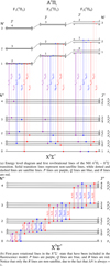 |
Fig. 1 Energy level diagram of the NH A3Πi − X3Σ−. |
4 Comparison with observational data and g factors
4.1 14NH
To check the accuracy of our 14NH model, we compared it to the very high-resolution, high S/N optical spectrum of Comet T7 as well as to the spectrum of the external comet F6, where “external” refers to comets that have a semimajor axis of a<10 000 au. The observed spectra of these two comets were taken at Rh = 0.68 au for T7 and Rh = 1.175 au for F6, giving us a large range of heliocentric distances to compare our model to. The high resolution allows us to analyze other bands besides the well-known (0–0) band. Figure 2 shows the (0–0) band of the 14NH fluorescence spectrum computed for the observational conditions of T7 (Fig. 2a) and F6 (Fig. 2b), respectively.
Combining the high-resolution spectrum of T7 and the new fluorescence model for 14NH has allowed us to identify new emission lines of the (0–1) band in the observational spectrum of T7 in the 3750 Å region. This weak band, never detected before, is shown in Figure 3. These lines are of low intensity, making them difficult to detect in the continuum-subtracted spectrum of T7. However, the confident identification of the strongest 14NH (0–1) lines supports the reliability of the detection.
We computed the total fluorescence efficiencies for the different bands up to v = 2, for a heliocentric distance of Rh = 1 au and a null heliocentric velocity of ![Mathematical equation: $\[\dot{R}_{h}\]$](/articles/aa/full_html/2025/10/aa55354-25/aa55354-25-eq18.png) = 0 km s−1. The values are given in Table 2. Our values are higher than the values found by Meier et al. (1998b) and Kim et al. (1989), which are around 6 × 10⁻¹⁴ erg s−1 molecule−1 for the (0–0) band. Meier et al. (1998b) reported ratios of g(1–1)/g(0–0) = 1 × 10⁻² and g(2–2)/g(0–0) = 8 × 10⁻⁶. The ratios we find are g(1–1)/g(0-0) = 7.2789 × 10⁻³ and g(2–2)/g(0–0) = 8.4206 × 10⁻⁵.
= 0 km s−1. The values are given in Table 2. Our values are higher than the values found by Meier et al. (1998b) and Kim et al. (1989), which are around 6 × 10⁻¹⁴ erg s−1 molecule−1 for the (0–0) band. Meier et al. (1998b) reported ratios of g(1–1)/g(0–0) = 1 × 10⁻² and g(2–2)/g(0–0) = 8 × 10⁻⁶. The ratios we find are g(1–1)/g(0-0) = 7.2789 × 10⁻³ and g(2–2)/g(0–0) = 8.4206 × 10⁻⁵.
Figure 4 depicts fluorescence efficiencies of the (0–0) band as a function of heliocentric velocities, ![Mathematical equation: $\[\dot{R}_{h}\]$](/articles/aa/full_html/2025/10/aa55354-25/aa55354-25-eq19.png) , and for different heliocentric distances, Rh. The fluorescence efficiencies have a high variability as a function of
, and for different heliocentric distances, Rh. The fluorescence efficiencies have a high variability as a function of ![Mathematical equation: $\[\dot{R}_{h}\]$](/articles/aa/full_html/2025/10/aa55354-25/aa55354-25-eq20.png) due to the Swings effect (Swings 1941), which is sensitive to the comet’s radial velocity with respect to the Sun. The trends seen in Figure 4 of the fluorescence efficiencies are in good agreement with the plots found in Meier et al. (1998b) and Kim et al. (1989) except that, again, our values are higher by about 20%.
due to the Swings effect (Swings 1941), which is sensitive to the comet’s radial velocity with respect to the Sun. The trends seen in Figure 4 of the fluorescence efficiencies are in good agreement with the plots found in Meier et al. (1998b) and Kim et al. (1989) except that, again, our values are higher by about 20%.
Figure 5 displays the ratio between the total fluorescence efficiencies of the (1–1) band and the total fluorescence efficiencies of the (0–0) band as a function of heliocentric velocities, ![Mathematical equation: $\[\dot{R}_{h}\]$](/articles/aa/full_html/2025/10/aa55354-25/aa55354-25-eq21.png) , and for different heliocentric distances, Rh. The overall values of this ratio are small because, as it was already noted in Table 2, the (0–0) band is ~137 times more intense than the (1–1) band.
, and for different heliocentric distances, Rh. The overall values of this ratio are small because, as it was already noted in Table 2, the (0–0) band is ~137 times more intense than the (1–1) band.
Table 3 regroups the wavelengths of the five most intense 14NH lines of the well-known (0–0) band for Rh = 1 au and ![Mathematical equation: $\[\dot{R}_{h}\]$](/articles/aa/full_html/2025/10/aa55354-25/aa55354-25-eq25.png) = 0 km s−1. This table also lists the most intense lines of the 14NH (0–1) band that has led to new line identification.
= 0 km s−1. This table also lists the most intense lines of the 14NH (0–1) band that has led to new line identification.
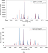 |
Fig. 2 14NH model compared to observed cometary spectra. The modeled spectra have been shifted by 0.3 Å to the left for clarity. Note that the prominent features of both the observed and the modeled spectra are the (0–0) band, but some weak lines of the (1–1) and (2–2) bands are also present in the 3340–3380 Å wavelength range. (a) Comparison between the modeled NH A3Πi − X3Σ− (0–0) band (red) and the observational spectrum of Comet C/2002 T7 (LINEAR) (blue) at a heliocentric distance of Rh = 0.680 au and a heliocentric velocity of |
![Mathematical equation: $\[\dot{R}_{h}\]$](/articles/aa/full_html/2025/10/aa55354-25/aa55354-25-eq15.png)
![Mathematical equation: $\[\dot{R}_{h}\]$](/articles/aa/full_html/2025/10/aa55354-25/aa55354-25-eq16.png)
Total band fluorescence efficiencies of 14NH.
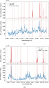 |
Fig. 3 New identification of the weak 14NH A3Πi − X3Σ−(0–1) band (red) in the observed spectrum of T7 (blue). Individual modeled emission lines of the (0–1) band are represented by the dashed red lines. (a) The most intense 14NH lines in the spectral region 3730–3750 Å are identified in the observed spectrum of T7. (b) The most intense 14NH lines in the spectral region 3750–3770 Å are identified in the observed spectrum of T7. |
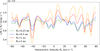 |
Fig. 4 Fluorescence efficiencies of the 14NH (0–0) band for different heliocentric velocities, |
![Mathematical equation: $\[\dot{R}_{h}\]$](/articles/aa/full_html/2025/10/aa55354-25/aa55354-25-eq22.png)
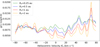 |
Fig. 5 Ratio of the g factors of the (1–1) band and the g factors of (0–0) band (g(1–1)/g(0–0)) of 14NH as a function of heliocentric velocity, |
![Mathematical equation: $\[\dot{R}_{h}\]$](/articles/aa/full_html/2025/10/aa55354-25/aa55354-25-eq23.png)
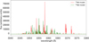 |
Fig. 6 Modeled 14ND spectrum in green compared to the modeled 14NH spectrum for Rh = 0.68 au and |
![Mathematical equation: $\[\dot{R}_{h}\]$](/articles/aa/full_html/2025/10/aa55354-25/aa55354-25-eq24.png)
4.2 14ND
Figure 6 compares the 14ND model to the 14NH model, where the relative intensities of the 14ND lines correspond to a hypothetical isotopic ratio, 14ND/14NH, of 1. The 14ND (0–0) band is intertwined with the 14NH (0–0), (1–1), and (2–2) bands, which makes the detection of the 14ND lines difficult.
Similarly to 14NH, we computed the fluorescence efficiencies of 14ND at a heliocentric distance of Rh = 1 au and a heliocentric velocity of ![Mathematical equation: $\[\dot{R}_{h}\]$](/articles/aa/full_html/2025/10/aa55354-25/aa55354-25-eq28.png) = 0 km s−1; they are shown in Table 4. Detailed 14ND line positions can be found in Table 3 and in the Supplementary Material.
= 0 km s−1; they are shown in Table 4. Detailed 14ND line positions can be found in Table 3 and in the Supplementary Material.
Most intense lines of NH.
Total band fluorescence efficiencies of 14ND.
4.3 15NH
Figure 7 compares the 15NH model to the 14NH model, with the relative intensities of the 15NH lines corresponding to a hypothetical isotopic ratio, 15NH/14NH, of 1. The 15NH model is shifted by 0.3 Å for clarity. Indeed, the 15NH lines are very close in wavelength to the 14NH lines. Figure 8 shows a zoom on a 2 Å-long region to highlight just how close the lines of the two isotopologs are (the intensities of both models have been shifted upward for readability). The brightest lines of 14NH and 15NH at 3358 Å are only separated by 0.008 Å.
Table 5 gives the fluorescence efficiencies of 15NH for all the bands with vibrational numbers up to 2 for a heliocentric velocity of ![Mathematical equation: $\[\dot{R}_{h}\]$](/articles/aa/full_html/2025/10/aa55354-25/aa55354-25-eq31.png) = 0 km s−1 and a heliocentric distance of Rh = 1 au. The same trends as in Section 4.1 apply for 15NH, meaning that the brightest band is the (0–0) one and that the (1–1) band is weaker by a factor of 100.
= 0 km s−1 and a heliocentric distance of Rh = 1 au. The same trends as in Section 4.1 apply for 15NH, meaning that the brightest band is the (0–0) one and that the (1–1) band is weaker by a factor of 100.
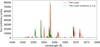 |
Fig. 7 Comparison between the modeled spectra of 14NH (red) and 15NH (green) for Rh = 0.68 au and |
![Mathematical equation: $\[\dot{R}_{h}\]$](/articles/aa/full_html/2025/10/aa55354-25/aa55354-25-eq29.png)
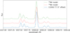 |
Fig. 8 Zoom on the most intense 14NH and 15NH line of the (0–0) band at 3358 Å. Both modeled spectra have been shifted to higher fluxes in order to visualize the small wavelengths shift between the 15NH and 14NH lines (therefore, no flux values are given). |
Total band fluorescence efficiencies of 15NH.
5 Measurements of isotopic ratios
5.1 14ND/14NH isotopic ratio
Meier et al. (1998b) determined an upper limit of 0.006 for the isotopic ratio 14ND/14NH in Comet C/1996 B2 (Hyakutake). We attempted to further constrain this ratio using our higher-resolution observational spectra and the new fluorescence models. The isotopic ratio measurement is enabled by the wavelength shift of the emission lines of both isotopologs, as is depicted in Figure 6. Because of the small 14ND/14NH ratio, 14ND lines are 103–104 times weaker than the bright 14NH lines. Therefore, in order to increase the S/N of the 14ND lines, we coadded a selection of 14ND lines. This 14ND line selection was based on two criteria: we wanted to select “bright” lines that are “not blended” with emission lines from other molecules. Based on the values of the fluorescence efficiencies given in Table 4 and the (0–0) band being the brightest one, the selected lines should be taken from the (0–0) band to increase the S/N as much as possible. Then, we compared the theoretical 14ND spectrum to the theoretical 14NH spectrum and to the observed spectrum in order to eliminate 14ND lines that are blended with 14NH lines or emission lines from other molecules. This significantly reduced the number of selected lines because, as is seen in Figure 6, the strong 14NH (0–0) band and weaker (1–1) and (2–2) bands are intertwined with the 14ND lines.
We were unable to retrieve an isotopic ratio from our observational spectrum of Comet T7 despite its high S/R. Indeed, T7 was observed at a short heliocentric distance of Rh = 0.68 au, meaning that it was very active at the time of observation. This activity may have created a very large number of weak, unidentified lines in the 3358 Å region. These lines could be the reason we do not manage to measure the isotopic ratio in these spectra. It is worth noting that the same spectra of T7 allowed a detection of OD to derive D/H = 2.5 ±0.7 × 10⁻⁴ in water. This measurement was compatible with other values of D/H in cometary water and marginally higher than the terrestrial value (Hutsemékers et al. 2008).
73P, on the other hand, was observed at a heliocentric distance of Rh = 0.952 au. This comet was found to be extremely depleted in carbon chains by Schleicher & Bair (2011), resulting in a spectrum that is less crowded in carbonated emission lines. This may be the reason we could retrieve an isotopic ratio from 73P and not from T7. Table 6 lists the ten 14ND lines that were chosen for coaddition as well as their 14NH counterparts.
The coaddition was performed following the method described by Jehin et al. (2004) and Hutsemékers et al. (2008). The result of the coaddition of the 14ND lines of Table 6 is shown in Figure 9. The coadditions of the 14NH counterparts are presented in Figure 10. The adjustment of the 14ND modeled intensity to the observational spectrum allows us to retrieve the isotopic ratio 14ND/14NH = 2.7 × 10⁻³ ± 1.8 × 10⁻³.
Several factors contribute to the uncertainty in our derived isotopic ratio. These include uncertainties in the energy levels and Einstein coefficients, the imperfect subtraction of the solar continuum, and the omission of collisional effects in our models (while previous studies found no evidence for collisional effects in NH fluorescence, the possibility that collisions could introduce second-order effects has been considered). While some of these sources are difficult to quantify, the dominant source of uncertainty comes from the background noise and the presence of a forest of weak, unidentified emission lines in the observed spectrum of 73P. To estimate this uncertainty, we measured the standard deviation, σ, in three spectral regions between 3320–3400 Å. Ideally, these regions would be free of emission lines, allowing us to isolate the noise. However, the 3320–3400 Å region is likely densely populated with weak, unidentified emissions, making it impossible to identify truly line-free intervals. As a result, our σ measurements inherently include contributions from these faint lines. We then weighted the measured noise by the same weights, wi, used for the coaddition of the observed emission lines. These weights are proportional to the modeled line intensities. By summing the products, σ × wi, across all selected lines, we obtained an estimate of the noise level in the coadded spectrum (shown in Figure 9). The final uncertainty in the isotopic ratio was determined by adjusting the model intensity to match this estimated coadded noise level.
Cometary D/H ratio are often compared to the terrestrial D/H value of ocean water of 1.557 × 10⁻⁴ given by the VSMOW (Vienna standard mean ocean water) (Gonfiantini 1978). The D/H ratio measured in cometary water varies from comet to comet, with, for example, D/H~2.1 × 10−4 measured in 1P/Halley (Brown et al. 2012) and D/H~5.3 × 10−4 measured in 67P/Churyumov–Gerasimenko (Altwegg et al. 2015). Cometary D/H ratios are generally higher for nitrogenated molecules compared to D/H in water. Indeed, (D/H)HCN~2.3 × 10−3 was measured in Comet Hale-Bopp (Meier et al. 1998a) and (D/HNH3~1.1 × 10−3 was measured with ROSINA in 67P/Churyumov–Gerasimenko (Altwegg et al. 2015). A comparison of our ratio, (D/H)NH ~ 2.7 × 10⁻³ ± 1.8 × 10⁻³, with the latter value found with ROSINA is especially interesting as NH3 is a parent molecule of the imidogen radical. The value we have found in 73P is in agreement with Altwegg et al. (2015)’s value for NH3 in comet 67P and with the upper limit, (D/H)NH ≤ 0.006, set by Meier et al. (1998b) in comet Hyakutake. As was noted by Meier et al. (1998a), the higher D/H ratios observed in nitrogen-bearing molecules relative to water suggest that cometary ices originated in the interstellar medium. This is consistent with the expectation that, in the cold environments of interstellar clouds, nitrogen-bearing species undergo more efficient deuteration than water.
Wavelengths in Å of the 14ND lines and their 14NH counter-parts coadded to measure the 14ND/14NH ratio.
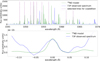 |
Fig. 9 Coaddition of 14ND lines. Top panel: 14ND lines selected for coaddition are indicated by vertical, dotted, purple lines listed in Table 6. The modeled 14ND spectrum in green has been intensified to have a flux similar to the observed spectrum of 73P in blue. Notice that some of the most intense lines of the 14ND modeled spectrum have not been selected for the coaddition, as they were blended with 14NH lines. Bottom panel: result of the coaddition of the 14ND lines of the observed spectrum of 73P in blue and the modeled 14ND lines in green. |
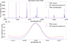 |
Fig. 10 Coaddition of 14NH counterparts. Top panel: 14NH counterparts indicated by vertical, dotted, purple lines. The modeled 14NH spectrum in red coincides for the most part with the observed spectrum of 73P in blue, as is discussed in Section 4.1. Bottom panel: result of the coaddition of the 14NH lines of the observed spectrum of 73P in blue and the modeled 14NH lines in red. |
5.2 15NH/14NH isotopic ratio
The method described in Section 5.1 of measuring isotopic ratios relies on the line shift between both isotopologs. However, as is seen in Figure 7, the shift between 14NH and 15NH lines is only 0.008 Å. The resolving power of the observed spectrum is R ~ 65 000, meaning that the resolution in terms of wavelengths is ![Mathematical equation: $\[\frac{\lambda}{R} \sim 0.052\]$](/articles/aa/full_html/2025/10/aa55354-25/aa55354-25-eq32.png) Å. Despite the exceptional quality of the observed spectra, their resolution is still not enough to measure the 15NH/14NH ratio.
Å. Despite the exceptional quality of the observed spectra, their resolution is still not enough to measure the 15NH/14NH ratio.
It is interesting to note that the carbon and nitrogen isotopic ratios were measured in 73P from the CN (0–0) violet band with values of 12C/13C = 100 ± 20 and 14N/15N = 215 ± 30 (Jehin et al. 2008). The nitrogen ratio appears to be significantly different from the average value of 147.8 ± 5.7 obtained from 23 comets of different origins and dynamical classes, while the carbon ratio is solar (89) and in agreement with the average value in comets (Manfroid et al. 2009).
6 Conclusions
Thanks to the spectroscopic data available in the Exomol database, we have been able to build new fluorescence models for 14NH, 14ND, and 15NH. The good match in terms of both the positions and the intensities of the lines between the modeled 14NH spectrum and our high-resolution and high S/N observational data of C/2002 T7 (LINEAR) and C/2012 F6 (Lemmon) allowed us to test the accuracy of the model. The modeling of the (0–1) band has led to new line identifications in the spectrum of C/2002 T7 (LINEAR). Additionally, the fluorescence efficiencies of the v′, v″ ≤ 2 have been tabulated and are found to be about 20% larger than in previous studies. These fluorescence efficiencies can be used to measure the NH abundances in comets. The 14ND model has allowed us to measure the 14ND/14NH ratio equal to 2.7 × 10⁻³ ± 1.8 × 10⁻³ in the periodic comet 73/P Schwassmann-Wachmann. This result is to be compared to the value of (D/H)NH ≤ 0.006 found by Meier et al. (1998b) in Comet C/1996 B2 (Hyakutake), (D/H)HCN ~2.3 × 10⁻³ found by Meier et al. (1998a) in Comet Hale-Bopp, and to the ratio D/H~1.1 × 10−3 in NH3 measured by the Rosetta mission on 67/P Churyumov–Gerasimenko (Altwegg et al. 2019). The value we have found is the first measurement of the D/H ratio in the NH radical and is consistent with the very few values already published for HCN and NH3. It confirms that the D/H ratio in nitrogen-bearing radicals is higher than the D/H ratio in water (1.5–6 × 10⁻⁴, Altwegg et al. 2015). No measurements could be carried out regarding the 15NH/14NH ratio, due to the limited shift between the lines of both isotopologs.
Acknowledgements
Based on observations collected at the European Southern Observatory, Paranal, Chile (ESO Programme 073.C0525). The datasets analyzed during the current study are available at the ESO Science Archive Facility at http://archive.eso.org/eso/eso_archive_main.html. E.J., D.H. and J.M. are Research Directors at the Belgian FRS-FNRS.
References
- Altwegg, K., Balsiger, H., Bar-Nun, A., et al. 2015, Science, 347, 1261952 [Google Scholar]
- Altwegg, K., Balsiger, H., & Fuselier, S. A. 2019, ARA&A, 57, 113 [NASA ADS] [CrossRef] [Google Scholar]
- Ballester, P., Modigliani, A., Boitquin, O., et al. 2000, The Messenger, 101, 31 [NASA ADS] [Google Scholar]
- Brown, R. H., Lauretta, D. S., Schmidt, B., & Moores, J. 2012, Planet. Space Sci., 60, 166 [NASA ADS] [CrossRef] [Google Scholar]
- Cochran, W. D. 1986, in ESA Special Publication, 250, ESLAB Symposium on the Exploration of Halley’s Comet, eds. B. Battrick, E. J. Rolfe, & R. Reinhard, 317 [Google Scholar]
- Delbouille, L., Roland, G., & Neven, L. 1973, Atlas photometrique du spectre solaire de [lambda] 3000 a [lambda] 10000 [Google Scholar]
- Gonfiantini, R. 1978, Nature, 271, 534 [CrossRef] [Google Scholar]
- Huebner, W. F., Keady, J. J., & Lyon, S. P. 1992, Ap&SS, 195, 1 [NASA ADS] [CrossRef] [Google Scholar]
- Hutsemékers, D., Manfroid, J., Jehin, E., Zucconi, J. M., & Arpigny, C. 2008, A&A, 490, L31 [NASA ADS] [CrossRef] [EDP Sciences] [Google Scholar]
- Jehin, E., Manfroid, J., Cochran, A. L., et al. 2004, ApJ, 613, L161 [Google Scholar]
- Jehin, E., Manfroid, J., Hutsemékers, D., et al. 2006, ApJ, 641, L145 [Google Scholar]
- Jehin, E., Manfroid, J., Kawakita, H., et al. 2008, in LPI Contributions, 1405, Asteroids, Comets, Meteors 2008, ed. LPI Editorial Board, 8319 [Google Scholar]
- Kim, S. J., A’Hearn, M. F., & Cochran, W. D. 1989, Icarus, 77, 98 [Google Scholar]
- Kurucz, R. L. 2005, Mem. Soc. Astron. Ital. Suppl., 8, 189 [Google Scholar]
- Litvak, M. M., & Kuiper, E. N. R. 1982, ApJ, 253, 622 [Google Scholar]
- Lockyer, N. 1912, Proc. Roy. Soc. Lond. A, 86, 258 [Google Scholar]
- Manfroid, J., Jehin, E., Hutsemékers, D., et al. 2009, A&A, 503, 613 [NASA ADS] [CrossRef] [EDP Sciences] [Google Scholar]
- Manfroid, J., Hutsemékers, D., & Jehin, E. 2021, Nature, 593, 372 [Google Scholar]
- Meier, R., Owen, T. C., Jewitt, D. C., et al. 1998a, Science, 279, 1707 [Google Scholar]
- Meier, R., Wellnitz, D., Kim, S. J., & A’Hearn, M. F. 1998b, Icarus, 136, 268 [Google Scholar]
- Perri, A. N., & McKemmish, L. K. 2024, MNRAS, 531, 3023 [Google Scholar]
- Schleicher, D. G., & Bair, A. N. 2011, AJ, 141, 177 [Google Scholar]
- Swings, P. 1941, Lick Observ. Bull., 508, 131 [Google Scholar]
- Swings, P., Elvey, C. T., & Babcock, H. W. 1941, ApJ, 94, 320 [NASA ADS] [CrossRef] [Google Scholar]
- Tennyson, J., Yurchenko, S. N., Zhang, J., et al. 2024, J. Quant. Spec. Radiat. Transf., 326, 109083 [NASA ADS] [CrossRef] [Google Scholar]
- Zucconi, J. M., & Festou, M. C. 1985, A&A, 150, 180 [NASA ADS] [Google Scholar]
All Tables
Wavelengths in Å of the 14ND lines and their 14NH counter-parts coadded to measure the 14ND/14NH ratio.
All Figures
|
Fig. 1 Energy level diagram of the NH A3Πi − X3Σ−. |
| In the text | |
|
Fig. 2 14NH model compared to observed cometary spectra. The modeled spectra have been shifted by 0.3 Å to the left for clarity. Note that the prominent features of both the observed and the modeled spectra are the (0–0) band, but some weak lines of the (1–1) and (2–2) bands are also present in the 3340–3380 Å wavelength range. (a) Comparison between the modeled NH A3Πi − X3Σ− (0–0) band (red) and the observational spectrum of Comet C/2002 T7 (LINEAR) (blue) at a heliocentric distance of Rh = 0.680 au and a heliocentric velocity of |
| In the text | |
|
Fig. 3 New identification of the weak 14NH A3Πi − X3Σ−(0–1) band (red) in the observed spectrum of T7 (blue). Individual modeled emission lines of the (0–1) band are represented by the dashed red lines. (a) The most intense 14NH lines in the spectral region 3730–3750 Å are identified in the observed spectrum of T7. (b) The most intense 14NH lines in the spectral region 3750–3770 Å are identified in the observed spectrum of T7. |
| In the text | |
|
Fig. 4 Fluorescence efficiencies of the 14NH (0–0) band for different heliocentric velocities, |
| In the text | |
|
Fig. 5 Ratio of the g factors of the (1–1) band and the g factors of (0–0) band (g(1–1)/g(0–0)) of 14NH as a function of heliocentric velocity, |
| In the text | |
|
Fig. 6 Modeled 14ND spectrum in green compared to the modeled 14NH spectrum for Rh = 0.68 au and |
| In the text | |
|
Fig. 7 Comparison between the modeled spectra of 14NH (red) and 15NH (green) for Rh = 0.68 au and |
| In the text | |
|
Fig. 8 Zoom on the most intense 14NH and 15NH line of the (0–0) band at 3358 Å. Both modeled spectra have been shifted to higher fluxes in order to visualize the small wavelengths shift between the 15NH and 14NH lines (therefore, no flux values are given). |
| In the text | |
|
Fig. 9 Coaddition of 14ND lines. Top panel: 14ND lines selected for coaddition are indicated by vertical, dotted, purple lines listed in Table 6. The modeled 14ND spectrum in green has been intensified to have a flux similar to the observed spectrum of 73P in blue. Notice that some of the most intense lines of the 14ND modeled spectrum have not been selected for the coaddition, as they were blended with 14NH lines. Bottom panel: result of the coaddition of the 14ND lines of the observed spectrum of 73P in blue and the modeled 14ND lines in green. |
| In the text | |
|
Fig. 10 Coaddition of 14NH counterparts. Top panel: 14NH counterparts indicated by vertical, dotted, purple lines. The modeled 14NH spectrum in red coincides for the most part with the observed spectrum of 73P in blue, as is discussed in Section 4.1. Bottom panel: result of the coaddition of the 14NH lines of the observed spectrum of 73P in blue and the modeled 14NH lines in red. |
| In the text | |
Current usage metrics show cumulative count of Article Views (full-text article views including HTML views, PDF and ePub downloads, according to the available data) and Abstracts Views on Vision4Press platform.
Data correspond to usage on the plateform after 2015. The current usage metrics is available 48-96 hours after online publication and is updated daily on week days.
Initial download of the metrics may take a while.