| Issue |
A&A
Volume 702, October 2025
|
|
|---|---|---|
| Article Number | A246 | |
| Number of page(s) | 18 | |
| Section | Extragalactic astronomy | |
| DOI | https://doi.org/10.1051/0004-6361/202556052 | |
| Published online | 30 October 2025 | |
Gravitational-wave background from extragalactic double white dwarfs for LISA
1
Laboratoire Lagrange, Observatoire de la Côte d’Azur, Université Côte d’Azur, CNRS, France
2
Artemis, Observatoire de la Côte d’Azur, Université Côte d’Azur, CNRS, CS 34229, F-06304 Nice Cedex 4, France
3
Dipartimento di Fisica “G. Occhialini”, Università degli Studi di Milano-Bicocca, Piazza della Scienza 3, 20126 Milano, Italy
4
INFN, Sezione di Milano-Bicocca, Piazza della Scienza 3, 20126 Milano, Italy
⋆ Corresponding author: This email address is being protected from spambots. You need JavaScript enabled to view it.
Received:
23
June
2025
Accepted:
16
August
2025
Abstract
Context. Recent studies have revealed that the contribution of extragalactic double white dwarfs (DWDs) to the astrophysical gravitational-wave background could be detectable in the millihertz regime by the LISA space mission. Conversely, the presence of this background could hamper the detection of cosmological backgrounds, which are among the key targets of gravitational-wave astronomy.
Aims. We aim to confirm the amplitude and spectrum of the extragalactic DWD background and estimate its detectability with LISA under different assumptions. We also aim to understand the main uncertainties in the amplitude and frequency spectrum and estimate whether the signal could be anisotropic.
Methods. We used the population synthesis code COSMIC with several assumptions about binary evolution and initial conditions. We also incorporated a specific treatment to account for the episodes of mass transfer and tidal torques after the formation of the DWDs.
Results. Our study is in global agreement with previous studies, although we find a lower contribution at high frequencies, due to a different treatment of mass transfer in stellar binaries. We find that the uncertainties in the amplitude are dominated by the star formation model, and to a lesser degree by the binary evolution model. The inclusion of tidal effects and mass transfer episodes in DWDs can change the amplitude of the estimated background up to a factor of 3 at the highest frequencies. For all the models we consider, we find that this background would be easily detectable, with signal-to-noise-ratio values from 100 to more than 1000 by LISA after 4 years of observations. Under the hypothesis of an homogeneous Universe beyond 200 Mpc, anisotropies associated with the astrophysical population of DWDs will likely not be detectable. We provide phenomenogical fits of the background produced by extragalactic DWDs under different assumptions to be used by the community.
Conclusions. We demonstrate significant variability in gravitational-wave background predictions, emphasizing uncertainties due to different astrophysical assumptions. We highlight the importance of determining the position of the knee in the gravitational-wave background spectrum, as it provides insights into mass transfer models. The prediction of this background is of critical importance for LISA in the context of observing other backgrounds.
Key words: gravitational waves / methods: statistical / binaries: close / white dwarfs
© The Authors 2025
 Open Access article, published by EDP Sciences, under the terms of the Creative Commons Attribution License (https://creativecommons.org/licenses/by/4.0), which permits unrestricted use, distribution, and reproduction in any medium, provided the original work is properly cited.
This article is published in open access under the Subscribe to Open model. This email address is being protected from spambots. You need JavaScript enabled to view it. to support open access publication.
1. Introduction
The Laser Interferometer Space Antenna mission (LISA), led by the European Space Agency (ESA), is designed to detect gravitational waves (GWs) in the frequency range [1 × 10⁻⁴, 1] Hz, with a projected launch in 2035 (Amaro-Seoane et al. 2018; Colpi et al. 2024). The diversity of sources detected by LISA will greatly enhance our understanding of both the broader cosmological properties of the Universe and the structure of our Galaxy. Aside from individually resolved sources, LISA is expected to observe several stochastic GW backgrounds (SGWBs) that result from the cumulative effect of numerous individual sources that are too faint to be resolved separately (Caprini & Figueroa 2018; Christensen 2018). This superposition produces a detectable background signal, quantified using the dimensionless parameter ΩGW, which represents the energy density of the SGWB with respect to the closure density of the Universe.
A guaranteed contribution to the SGWB comes from the superposition of unresolved compact binaries within our Galaxy, primarily double white dwarfs (DWDs). The confusion signal they create is known as the Galactic foreground (Ungarelli & Vecchio 2001; Nissanke et al. 2012; Boileau et al. 2021; Karnesis et al. 2021; Toubiana et al. 2024; Buscicchio et al. 2025; Criswell et al. 2025). This foreground is challenging to analyze due to its observed non-stationarity caused by LISA’s orbit in combination with the shape of the Milky Way. On the other hand, this annual modulation aids in its separation from the other, isotropic, backgrounds when analyzing LISA data.
An isotropic cosmological SGWB is anticipated to originate from a variety of processes in the early Universe (Caprini et al. 2009; Christensen 2018; Mazumdar & White 2019; Auclair et al. 2023), whose signals may combine into a single background. Detecting this cosmological SGWB is one of the key scientific objectives of LISA, but such a signal must be carefully disentangled from other astrophysical backgrounds. Spectral separation techniques (such as parametric estimation) can help isolate individual components of the SGWB. In this context, Bayesian inference provides a model-dependent framework that combines prior knowledge with observational data to update the probability distributions of hypotheses or model parameters. For such methods to succeed, all non-cosmological contributions to the SGWB must be accurately characterized and parametrized.
For instance, an isotropic astrophysical SGWB is expected, due to the superposition of GWs emitted by inspiraling compact binaries throughout the Universe. Observations by the LIGO/Virgo/KAGRA collaboration (LVK) have provided an upper limit on the contribution to the astrophysical GW background coming from binaries containing black holes and/or neutron stars (Chen et al. 2019; Abbott et al. 2021).
Extragalactic DWDs are also expected to contribute to the astrophysical SGWB, but major uncertainties remain regarding their contribution, since this population of sources is not observable by any current facility. They were first introduced in Schneider et al. (2001), and Farmer & Phinney (2003) later estimated the SGWB they produce, obtaining ΩGW(1 mHz)∈[1, 6]×10−12.
Recently, Staelens & Nelemans (2024) revisited this estimate, finding a 60% higher amplitude than previous models, and concluding that DWDs likely dominate the SGWB in this frequency range. The following study by Hofman & Nelemans (2024) examined the impact of the stellar metallicity, star formation rate density (SFRD), and binary evolution models, finding that the SGWB produced by extragalactic DWDs can vary by up to a factor of 5, but consistently remains the primary source detectable by future detectors like LISA, dominating the contribution from binaries made of black holes and/or neutron stars. Thus, the extragalactic DWD background appears to be a guaranteed LISA source, which will impact the detectability of other sources, in particular the cosmological SGWB.
This paper presents an alternative study of the modeling and understanding of the SGWB from extragalactic DWDs. In the method section (Sect. 2), we describe the LISA context, the theoretical framework for SGWB modeling, the population synthesis of DWD, and the development of a dedicated code to compute the SGWB from extragalactic DWDs. The results section (Sect. 3) starts with a validation of our model against previous studies, an analysis of how stellar evolution assumptions affect the resulting DWDs population, and investigations of the impact of taking into account matter interactions within DWDs on the SGWB and of potential anisotropies in the SGWB from extragalactic DWDs signal. In the discussion (Sect. 4) we explain the limits of our model and comment on the observability of the background. The conclusions (Sect. 5) synthesizes our findings and suggests future research directions to deepen our understanding of the SGWB. In all our subsequent calculations, we adopt the cosmological parameters from the Planck 2018 results (Planck Collaboration VI 2020), with best-fit parameters of H0 = 67.66 km s−1 Mpc−1, Ωm = 0.30966, and TCMB = 2.7255 K.
2. Method
In this work, we estimate the contribution of extragalactic DWDs to the SGWB detectable by LISA. Section 2.1 sets the mission context, including instrument and observation assumptions. Section 2.2 outlines the theoretical framework and SGWB energy density equations. In Section 2.3, we present the population synthesis models for DWDs. Section 2.4 describes how these models are combined with various cosmic star formation histories to compute the SGWB from extragalactic DWDs.
2.1. LISA sensitivity to stochastic backgrounds
We adopt the sensitivity curve corresponding to an equilateral triangle with stationary instrumental noise, as described in the LISA red book (Colpi et al. 2024; Thorpe et al. 2019). This assumption allows us to directly model the SGWB signal without any need for additional instrumental corrections.
It is standard practice to express the signal in terms of the GW energy density power spectrum, which can be related to the GW strain power spectral density. We introduce the energy density sensitivity Ωs(f), which is determined by the sensitivity of the detector’s strain measurements  where Sn(f) represents the noise power spectral density of the detector,
  the LISA response function (Babak et al. 2021) and NX(f) the power spectral density of the LISA noise X Channel (Tinto et al. 2004).
For the rest of the paper we assume the equal correlation hypothesis and the LISA noise model is given by the power-law integrated sensitivity (PI curve, following Thrane & Romano 2013) for four years of observation time and a fixed value of 10 for the signal-to-noise ratio (S/N; solid gray line in the gray solid line on figures, see e.g., Babak et al. 2021). The PI curve is a graphical tool used to represent the sensitivity of GW detectors to stochastic backgrounds characterized by power-law spectra. It indicates the minimum energy density of a stochastic background that a detector can observe across different spectral ranges, assuming the background is isotropic, stationary, and Gaussian.
While the PI curve is a valuable tool for assessing detector sensitivity to idealized SGWBs, its application to specific cases such as LISA presents limitations. LISA is a unique space-based detector with arms forming an equilateral triangle and collocated interferometers, which implies distinct challenges compared to ground-based detectors. Moreover, certain astrophysical SGWBs, such as those from extragalactic white dwarf binaries, may deviate from the assumptions of the powerlaw spectrum, isotropy, stationarity, and Gaussianity. Consequently, more specialized analysis methods are necessary to evaluate the detectability of such backgrounds with LISA. In particular, two key limitations arise when applying the PI approach to the SGWB from extragalactic DWDs. First, the background is not stationary: the Galactic foreground contributing to the signal is modulated over the course of a year due to LISA’s orbital motion. Second, the spectral shape of the SGWB from extragalactic DWDs is not a simple power-law, as typically assumed in PI analyses, but results from a complex population synthesis shaped by astrophysical processes. Consequently, more specialized analysis methods are necessary to evaluate the detectability of such backgrounds with LISA. The PI curve has often been used as a standard framework in previous studies to evaluate LISA’s sensitivity. In our case, we include it solely to enable comparison with earlier work. We do not interpret it further, as it does not reflect the physical complexity of the SGWB from extragalactic DWDs.
The confusion noise generated by unresolved galactic DWD systems was modeled from Robson et al. (2019) as
![Mathematical equation: $$ \begin{aligned} S_c(f) = A f^{7/3}_{\text{Hz}} e^{-f_{\text{ Hz}} \alpha + \beta f_{\text{ Hz}}\sin (\kappa f_{\text{ Hz}}) } \left[1 + \tanh \left(\gamma (f_k - f_{\text{ Hz}})\right)\right] , \end{aligned} $$](/articles/aa/full_html/2025/10/aa56052-25/aa56052-25-eq3.gif) (1)
(1)
where fHz = f/(1 Hz), with the parameters α = 0.138, β = −221, γ = 1680, and fk = 0.00113. The corresponding dimensionless energy spectral density can be determined from ΩGW, c(f) = 4π2Sc(f)f3/(3H02).
Using the latest estimates from the LVK Collaboration, we model the total contribution of black hole binaries, neutron star binaries, and black hole-neutron star binaries to the SGWB as the normalized energy density ΩNS/BH(f) such that
 (2)
(2)
with  (Abbott et al. 2023).
2.2. SGWB formalism and computation
The SGWB generated by compact binaries comes from the superposition of a large number of weak, independent, and unresolved sources. Its energy-density spectrum can be characterized by the dimensionless quantity (Allen & Romano 1999):
 (3)
(3)
where dρGW is the energy density of this background signal within the frequency range [ f,f+df [, and c is the speed of light. ρc = 3H02/8πG is the critical energy density of the Universe, where H0 is the Hubble-Lemaitre constant and G the gravitational constant.
In a homogeneous, isotropic, and expanding Universe, the dimensionless energy spectral density, ΩGW, measured today can be expressed as (Phinney 2001; Regimbau & Mandic 2008)
 (4)
(4)
where fe = fr(1 + z) is the GW frequency of a source in its rest frame, and dEGW/dfe is its energy spectrum. The function N(z) denotes the number of such sources emitting GWs at frequency fe per unit redshift and per unit comoving volume.
Following (Farmer & Phinney 2003), Eq. (3) can be rewritten considering a SGWB produced by binaries and in terms of specific flux development as
 (5)
(5)
where Ffr is the specific flux received in GWs today at frequency fr. In the case of a single source located at redshift z and emitting GWs at a frequency, fe, with a specific luminosity, Lfe, this specific flux reads
 (6)
(6)
where dL(z) is the luminosity distance to the source located at redshift z. In reality, the SGWB from extragalactic DWDs emanates from an immense number of sources located over a large redshift range, and Ffr is the sum of the specific fluxes of all these individual systems. Staelens & Nelemans (2024) find that the number of DWDs making up this GW background can be as high as 1017. As it is impossible to simulate all these sources and compute the actual discrete sum of all their contributions, we make the assumption that they are isotropically distributed over the sky and express the specific flux as
 (7)
(7)
where lfe(z) is the specific luminosity density of sources at redshift z emitting with a GW frequency fe and dV(z) is the comoving volume element at redshift z. dχ(z) is the comoving distance and dV(z) = 4πdM(z)2dχ(z) with dM(z) the proper motion distance such that dL(z) = (1 + z)dM(z). This formula expresses the idea that the GW flux received in the present-day at a given frequency, fr, can originate from sources at all redshifts, with various emitting frequencies, fe, which are redshifted to reach us observers with the frequency, fr, following fe = (1 + z)fr.
We note here that, in this work, we do not take into consideration the contribution from any particular galaxy, such as the Milky Way or satellite galaxies (Pozzoli et al. 2025). The computation of the SGWB is entirely based on the assumption of isotropic homogeneous Universe at all scales. We will see later (see Sect. 3.4) that, even though this assumption does not hold at the lowest redshifts, the SGWB is almost entirely dominated by sources at redshifts where the Universe can be considered as such, and that the treatment of local galaxies would have only a very minor effect.
To estimate the energy-density spectrum of the SGWB from extragalactic DWDs, we discretized the integral in Eq. (7). We split the redshift range from z = 0 to z = 8 in 20 bins corresponding to a linear spacing in lookback time, and the received GW frequencies were logarithmically spaced in 50 bins between 10−5 Hz and 10−1 Hz. For readability purposes, in all the figures showing ΩGW(f) we only plot half of the frequency bins in the range [5 × 10⁻⁵, 5 × 10⁻²] Hz. The total flux received in any frequency bin [fr1,fr2] can now be expressed in the discrete form:
 (8)
(8)
We next evaluated the specific luminosity density, lfe, in our different redshift bins and for each frequency bin, [fr1,fr2], in order to compute the fluxes Ffr1 → fr2 and finally ΩGW. We used catalogs of DWDs generated through population synthesis (described in further details in Sect. 2.3) and estimated the specific luminosity density as Staelens & Nelemans (2024)
 (9)
(9)
where dEGW/dfe(k) is the energy spectrum of the DWD k emitting GWs at frequency fe, ḟe(k) is its frequency evolution, and nk(fe, z) is the specific number density of such system at redshift z.
The energy spectrum can be approximated by the leading quadrupole order in the GW emission (Hawking & Israel 1987)
 (10)
(10)
where ℳc is the chirp mass of the system k. It is defined as ℳc = (m1m2)3/5/(m1 + m2)1/5, with m1 and m2 the two DWD masses.
The specific number density can be written as
 (11)
(11)
with ℛk(fe, z) the rate density at which systems k start emitting GWs at a frequency, fe, at redshift z. In the following subsections Sects. 2.3 and 2.4, we present how we combined results from population synthesis with a cosmological star formation history to compute these factors, ℛk(fe, z).
The dimensionless energy density can finally be expressed using this total flux of GWs received in the frequency bin [fr1,fr2] as
 (12)
(12)
where  is the mean frequency of the frequency bin [fr1,fr2].
In order to assess the detectability of the SGWB from extragalactic DWDs, we computed the S/N following following (Smith & Caldwell 2019)
 (13)
(13)
where Tobs = 4 and 10 years is the observation time and Ωsens(f) is the effective sensitivity that includes LISA’s instrumental noise and the Galactic confusion noise,
 (14)
(14)
2.3. Population synthesis of DWDs with COSMIC
In this study, we used the rapid binary population synthesis code COSMIC (Breivik et al. 2020) to simulate the evolution of isolated stellar binaries leading to the formation of DWDs. COSMIC is a code directly adapted from the binary stellar evolution code (Hurley et al. 2002), with many additional prescriptions. The most relevant one for WD progenitors is the model of mass loss through stellar winds (e.g., Vink et al. 2001; Vink & de Koter 2005). As was described in Hurley et al. (2002), the stability of mass transfer is determined in COSMIC using values of critical mass ratios qcrit = mdonor/maccretor (see e.g., Hjellming & Webbink 1987) and the phase of common envelope (CE) evolution is modeled with the standard αλ energy formalism (see e.g., Ivanova et al. 2013). In this formalism, λ represents a binding energy factor of the envelope to the binary and the parameter α describes the efficiency with which orbital energy can be transferred to the envelope, eventually ejecting it if a sufficient amount of energy is passed on.
In our default set of population synthesis prescriptions, each stellar population that we simulated was initialized following the Kroupa (2001) initial mass function (IMF) between 0.08 and 150 M⊙. After individual stellar masses had been drawn from this distribution, each star was associated with a companion or not according to the mass-dependent binary fraction  , for 0.08 ≤ M/M⊙ ≤ 100 (van Haaften et al. 2013). We assumed that all stars more massive than 100 M⊙ have a companion. Higher-order multiple systems were not considered here. Companion masses were sampled following a uniform distribution for the mass ratios q = M2/M1 (Goldberg & Mazeh 1994). We used the distributions inferred in Sana et al. (2012) for orbital separations and eccentricities. To take into account the effect of metallicity on binary evolution and the formation of DWDs, we initialized and evolved stellar populations with 25 different metallicities, uniformly log-spaced such that the central values cover the range [10−2, 1] Z⊙, where we assume Z⊙ = 0.017 after Grevesse & Sauval (1998).
One particular feature of COSMIC is that the size of the total simulated population of stellar binaries can be set as a free parameter and determined over the course of each run. This allows COSMIC to continue initializing and evolving new binaries until the physical properties of the final population of DWDs have reached a certain convergence (we refer the reader to Breivik et al. 2020, for details on the convergence criterion, which we have set to a value of –5 here). As such, we warn the reader that the total number of DWDs obtained for one given run is not a representative quantity, but the total size of the simulated stellar population should also be taken into account when comparing results from different COSMIC models.
For the different prescriptions used to simulate stellar evolution and binary interactions, we followed, for the most part, the set of physical prescriptions proposed on the COSMIC GitHub. Regarding the phase of CE evolution, we consider a binding energy factor, λ, which depends on stellar types following Claeys et al. (2014) and an efficiency parameter α = 1.
Aside from out default model, we consider three additional models to measure the importance of the characteristics of the initial stellar population and of the prescriptions used to model their evolution. In fb1, we assume that all stars are born in binaries, i.e. that, regardless of the mass, the binary fraction is fb = 1. This model serves as an extreme case for quantifying the uncertainty in the binary fraction during the astrophysical processes of star formation. In multidim, the initial binary parameters are no longer sampled sequentially, as in the default model described above, but all at once using the multidimensional distribution functions described in Moe & Di Stefano (2017). Finally, in order to quantify some of the uncertainties during binary evolution and for the sake of comparison with Staelens & Nelemans (2024), Hofman & Nelemans (2024), we also run a series of COSMIC simulations with a CE efficiency parameter α = 4 (in what follows, this model is referred to as α4). A higher value of α means that energy is transferred more efficiently to the envelope. It is therefore ejected more easily and this typically results in post-CE systems with greater orbital separations, i.e lower GW frequencies at formation.
As we are interested in the DWDs that contribute to the SGWB detectable with LISA, and in order to reduce the size of the large populations of DWDs simulated with COSMIC, we apply a frequency threshold to select only the systems which, in the course of their evolution, have a chance of passing through the LISA frequency band (0.1 mHz to 1.0 Hz with a GW strain spectral density 10−21 to 10−23, Colpi et al. 2024). In practice, we select the systems that would have a redshifted GW frequency higher than 10−6 Hz at redshift z = 10.
For each WD in a binary, we look at the composition of its core and whether it is made of helium (He), carbon-oxygen (CO), or oxygen-neon (ONe). The number of each type of DWD formed at solar metallicity with our different COSMIC set of models in are presented in Table 1.
Total number of DWDs and stellar mass for different COSMIC models.
The diversity in WD core composition arises from the dependence of stellar core evolution on the progenitor’s initial mass. Stars with initial masses ≲2.2 M⊙ evolve into helium-core WDs, while intermediate-mass stars (∼2.2 to ∼6.5 M⊙) undergo helium and hydrogen shell burning eventually forming carbon-oxygen WDs. More massive stars (≳6.5 M⊙), depending on metallicity and convective over shooting, can ignite carbon and form oxygen-neon cores before envelope loss or collapse (Althaus et al. 2010).
It is important to note here that these numbers for DWDs do not account for any assumption on the cosmic star formation history or on the metallicity distribution across time in the Universe. They represent the catalog of all the DWDs simulated with Z⊙ after applying the low-frequency cutoff. In our default model, the majority of systems are CO-He pairs (∼58%), followed by CO-CO (∼26%) and He-He pairs (∼13%). As they originate from more massive stars, the systems containing at least one ONe WD are naturally less common (∼3% in total), with the rarest being the ONe-ONe pairs.
As the three models default, fb1, and multidim, use the exact same prescriptions to describe binary evolution but differ only in the properties of their initial stellar populations, they predict comparable relative numbers of each type of DWD. On the other hand, the COSMIC model α4 using a higher CE efficiency parameter results in an overall larger efficiency for forming DWDs in the considered frequency range, and in notable differences in the relative number of types of DWDs. This can be explained by the fact that, with a higher efficiency at ejecting the envelope, more systems can survive this phase of unstable mass transfer. More He-He systems are formed in this case. More details on the physical properties of the DWDs at the time of their formation and on the formation efficiency between our different COSMIC models are presented in Appendix A.1.
2.4. Procedure for estimating the SGWB from extragalactic DWDs
2.4.1. Metallicity-specific SFRD
In order to estimate the rate density factors ℛk(fe, z) in Eq. (11) at different redshifts and for different emitting frequencies, we relate the formation of DWDs to the formation of stars in the Universe. Throughout this study, we make the assumption that the metallicity-specific SFRD can be split in two different independent factors:
 (15)
(15)
where ψ(z) is the cosmological SFRD as a function of redshift and dP/dZ indicates the metallicity distribution function.
We used a single model here for the metallicity distribution function dP/dZ, taken as the “preferred model” presented in Neijssel et al. (2019). To take account of certain observational uncertainties in the SFRD, particularly at high redshifts, we use three different models here: the classic SFRD from Madau & Dickinson (2014), an updated empirical determination from Madau & Fragos (2017), and a parametric form in time from Strolger et al. (2004). Following Madau & Dickinson (2014) and Madau & Fragos (2017), the SFRD as a function of redshift can be expressed as
![Mathematical equation: $$ \begin{aligned} \psi (z) = a \frac{(1 + z)^b}{1 + [(1 + z)/c]^d}\,{\mathrm{M} _\odot }\,\mathrm{yr} ^{-1}\,\mathrm{Mpc} ^{-3}. \end{aligned} $$](/articles/aa/full_html/2025/10/aa56052-25/aa56052-25-eq21.gif) (16)
(16)
Alternatively, Strolger et al. (2004) parametrized the SFRD as a function of cosmic time (expressed in gigayears) as
 (17)
(17)
where t0 is the current age of the Universe (set in their fit at 13.47 Gyr).
Combining the results of our population synthesis of DWDs carried out using COSMIC (Sect. 2.3) with the models of metallicity-dependent star formation presented here, we can now estimate the rate density at which systems, k, start emitting GWs at a frequency, fe, at redshift z as
 (18)
(18)
where Δz indicates the variation in redshift corresponding to the time elapsed from the formation of the progenitor stellar binaries until the remnant DWD k has evolved to emit GWs at frequency fe at redshift z, and MSF(Z) is the total initial mass of the stellar population simulated with COSMIC at metallicity Z.
More details on these models of SFRD and on the metallicity distribution function are presented in Appendix A.2. The best fit parameters for Eqs. (16)–(17) can be found in Table A.1. In Appendix A.3 we also show that metallicity has a limited impact on DWD formation.
2.4.2. Orbital evolution with GW emission
In the Newtonian limit, the orbital frequency of a binary system is given by
 (19)
(19)
where a is the semimajor axis of the orbit. For quasi-circular systems, the GW emission frequency of a binary relates to its orbital frequency as fe = 2 × forb.
Under the simplified assumption that the binary evolves purely by GW emission, the frequency evolution follows (Farmer & Phinney 2003)
 (20)
(20)
where
 (21)
(21)
By default, we considered that when one of the two WDs fills its Roche lobe, meaning that its radius extends beyond the surface inside which matter is gravitationally bound to it, the DWD merges and the system does not contribute to GW emission anymore (Lamberts et al. 2019). As such, we determined a maximum orbital frequency, and therefore a maximum GW emission frequency fe, max, for each system in our catalog. We discuss in the following subsection (Sect. 2.4.3 an alternative treatment taking into account the interaction between WDs.
To compute the Roche lobe effective radius for the WD identified by the index 1, we used the approximation from Eggleton (1983)
 (22)
(22)
where 0 < q = M1/M2 < ∞ and a is the orbital separation of the binary. The minimum orbital separation that a binary can reach before one of its two components fills its Roche lobe is then given by a = max(RWD, 1/RL, 1, RWD, 2/RL, 2), where RWD, 1 and RWD, 2 are the radii of the two WDs.
From Eq. (21), we can then derive the time elapsed from the formation of a DWD until it reaches a given GW frequency fe < fe, max, as
 (23)
(23)
where fe, 0 is the binary initial GW frequency.
In the case of evolution through GW emission only, we combined for each system the time delay from the progenitor stellar binary to DWD formation predicted by COSMIC with the above expression of Δt to estimate in Eq. (18) the equivalent z + Δz for different GW frequencies and different redshifts. For the systems that can never emit GWs at frequency fe at redshift z, because it would take too long to reach this frequency, or they would merge before, or they form already at a higher frequency, we used ℛ(fe, z) = 0.
2.4.3. Treatment of interacting DWDs
In the case in which we consider mass transfer and tidal effects during the evolution of DWD systems, the chirp mass is no longer constant and both ℳc(t) and fe(t) do not have analytical expressions. We evolved each DWD using the model of Toubiana et al. (2024) and recovered the simulated evolutions of ℳc(t), fe(t), and ḟe(t).
In short, when the two WDs are close enough together, the lighter one, which is also the largest one, can overfill its Roche lobe and start transferring mass to the heavier one. An intense mass-transfer episode occurs, which may cause a prompt merger. In our model, this occurs if the mass-transfer rate exceeds 10−2 M⊙ yr−1. Binaries that survive this mass transfer start out-spiraling. In some rare cases, the donor can successively overfill and underfill its Roche lobe, causing the orbital separation to oscillate, until the binary definitely out-spirals.
To compute the integral of Eq. (8), we performed a change of variable as fe → t such that
 (24)
(24)
Binaries that out-spiral can contribute multiple times to the same frequency bins. To account for that effect, we used our numerical solution of fe(t) to identify each occurrence of the binary crossing a given frequency bin and then summed the contribution of each of those passages as the integral in Eq. (24). Each of the contributions was weighted by the corresponding factor defined in Eq. (18), where Δz is the redshift variation corresponding to the time elapsed between the formation of the progenitor stellar binaries and that passage of the binary in the frequency bin.
Unless otherwise specified, we always used the first simplified case throughout this paper and assumed that DWD evolution is driven by GWs only, neglecting all the potential episodes of mass transfer and tidal interactions. The effects of this more realistic treatment are explored in Sect. 3.3.
3. Results
3.1. Predictions for the SGWB from extragalactic DWDs
In Fig. 1, we show the spectral energy density obtained with our four different COSMIC models (see Table 1) using our default SFRD model (Madau & Dickinson 2014). We find consistent predictions across our different population synthesis models, although not exactly similar. In particular, with a fixed SFRD model, the SGWB obtained with the COSMIC model alpha4 is 2–4 times higher than the other three models in the frequency band [5 × 10⁻⁴, 5 × 10⁻³] Hz. This difference is a direct consequence of the higher efficiency at forming DWDs with this model (see Fig. A.3). With a similar approach and using different models of CE evolution, Hofman & Nelemans (2024) report a factor of ∼2 between their highest and lowest estimates of the SGWB from extragalactic DWDs at a fiducial frequency of 1 mHz.
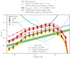 |
Fig. 1. Spectral energy density of the SGWB from extragalactic DWDs for various population synthesis models (see Sect. 2.3) and various SFRD models (see Sect. 2.4.1). The different population synthesis models are indicated with the same markers as in Fig. A.3. Dotted, solid, and dashed lines correspond to the SFR models from Strolger et al. (2004), Madau & Dickinson (2014), and Madau & Fragos (2017) respectively. The black line represents the LISA sensitivity curve (Colpi et al. 2024), while the gray one shows the PI curve (Thrane & Romano 2013) for four years of observation time and S/N = 10. The light blue curve is the confusion noise from Galactic DWDs (Robson et al. 2019) and the green green band is the 90% credible interval of the SGWB from all compact object binaries estimated from observations of GWs (Abbott et al. 2023). As a comparison, the shaded blue band shows the SGWB from extragalactic DWDs estimated in (Farmer & Phinney 2003) and the pink curve indicates the best-fit model obtained in (Staelens & Nelemans 2024). In Appendix B, we discuss and summarize the fits of SGWB from extragalactic DWDs of all SFR models and stellar population synthesis models as presented in Table B.1. |
The spread arising from the different population synthesis models is fairly similar across the different SFRD models and remains consistent with our previous description using the default SFRD model from Madau & Dickinson (2014). It is clear that the choice of SFRD model has a major impact on the global amplitude of the SGWB from extragalactic DWDs. Indeed, as the fraction of stellar binaries that evolve to become DWDs is roughly constant over a large range of metallicities (see Fig. A.3), the amplitude of the SGWB from extragalactic DWDs naturally relates to the total mass of stars that have formed in the entire history of the Universe, or the integrated star formation rate (SFR). As the SFRD model from Strolger et al. (2004) predicts notably more star formation at z > 2 than the two other SFRD models (see the left-hand panel of Fig. A.4), this naturally translates into much higher SGWB amplitudes. We find that the use of different SFRD models dominate the uncertainty in the SGWB amplitude, with a factor of up to 6–7, while different models of initial stellar populations and of binary evolution have a more moderate impact, with variation by a factor of 2–3 in the global amplitude of the predicted SGWB. This variation highlights the strong sensitivity of the SGWB from extragalactic DWDs predictions to assumptions about the CE phase and the global SFR.
In addition to modeling uncertainties, observational limitations must be considered. The Galactic foreground dominates the sub-milliHz regime and decreases steeply above ∼2 mHz, while the extragalactic signal becomes most prominent between ∼3 and 7 mHz. Although the two components occupy partially distinct frequency ranges, their overlap at intermediate frequencies can still challenge signal separation. Extending the observation time improves sensitivity, but does not fully resolve the ambiguity between overlapping astrophysical contributions without additional constraints or targeted analysis techniques.
We compared our results with previous studies (shaded blue area and pink curve, corresponding to Farmer & Phinney 2003; Staelens & Nelemans 2024, respectively) and found a consistent overall picture. In particular, Staelens & Nelemans (2024) use the same SFRD model from Madau & Dickinson (2014) and simulate DWD formation with the population synthesis code SeBa (Portegies Zwart & Verbunt 1996; Nelemans et al. 2001; Toonen et al. 2012). As we have used different codes and different physical prescriptions for certain treatments of binary interactions, it does not come as a surprise that we do not find an exact match to their predictions. However, one very notable observation is the difference in the location of the frequency cutoff. While Staelens & Nelemans (2024) find a decrease in the energy density spectrum for frequencies above fc ∼ 20 mHz, all our models predict a sharp drop-off at a lower frequency fc ∼ 7 mHz. We explore the origin of this discrepancy at high frequencies in detail in the discussion section (see Section 4.1).
These results underscore the significant importance of the assumptions made on star formation, stellar evolution, and binary interactions to predict a SGWB and their relevance for future GW observations. Apart from its global amplitude, we find no other distinguishable effect of the SFRD model on the SGWB from extragalactic DWDs. For comparison, we also report in green the astrophysical SGWB expected from compact binaries composed of black holes and/or neutron stars, based on the LVK observations. In all our models, the contribution from extragalactic DWDs dominates in the LISA range.
Our predictions for the SGWB of extragalactic DWDs come very close to the LISA sensitivity curve (black curve) in the frequency band [2 × 10⁻³, 8 × 10⁻³] Hz, and even distinctly above for the most optimistic COSMIC model alpha4. This suggests that the LISA mission may allow us to put some strong observational constraints on the amplitude of this SGWB in this frequency range.
Signal-to-noise ratio (S/N) for each SFR and population synthesis model.
Table 2 shows that the computed S/N varies by more than an order of magnitude across models, from ∼100 for conservative scenarios (e.g., default + Madau Fragos) up to nearly ∼1500 (e.g., alpha4 + Strolger) for a 4-year mission, and reaching ∼2400 for a 10-year observation in the most favorable case. Even scenarios involving the default model paired with the Madau & Dickinson (2014) or Madau & Fragos (2017) SFR yield S/N values well above unity ranging from ∼100 to ∼400 for T = 4 yr and up to ∼600 for a 10-year mission. These very high S/N values demonstrate that , in all scenarios, the detection of the SGWB from extragalactic DWDs by LISA is virtually guaranteed (see Table 2), regardless of Galactic foreground or instrumental sensitivity limits. However, the degeneracies between the effect of the cosmological SFRD, the properties of initial stellar populations, and the nature of CE evolution will remain challenging to disentangle, as detection alone will not suffice to constrain these physical processes independently. These fundamental uncertainties in binary evolution modeling and star formation histories will affect the interpretation and parameter inference of the observed background. Therefore, while extending the observation period further increases S/N, the focus should shift toward accurately modeling these astrophysical uncertainties to fully exploit the detection, notably the position of the typical frequency at which the signal starts to drop, referred to here as the knee, which will have an impact on the astrophysical models. Furthermore, if the SFRD turns out to be larger at high redshifts than the commonly used model of Madau & Dickinson (2014), then the SGWB from extragalactic DWDs could have an even stronger impact on the effective sensitivity curve of LISA, particularly in the frequency band [10−3, 10−2] Hz.
3.2. Contribution of different DWD types to the SGWB
Fig. 2 shows the energy density spectrum for the various types of DWDs, using our default COSMIC model and the SFRD from Madau & Dickinson (2014). Across most of the frequency range the SGWB is dominated by CO-He sources. This is naturally expected from the high formation efficiency of this type of DWD compared to the other types (see Table 1 and e.g., Lamberts et al. 2019).
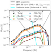 |
Fig. 2. Spectral energy density of the SGWB from extragalactic DWDs for the various types of DWDs, with our default COSMIC model and the SFRD from Madau & Dickinson (2014). Different colors indicate the contribution from different type of DWD binaries. We do not show the contribution of ONe-ONe binaries here, as it is several orders of magnitude below due to their rarity. The sum of all the contributions is shown in black. Additional curves represent the LISA sensitivity, the PI curve, and the confusion noise from Galactic DWDs. |
At higher frequencies (fGW, r ≥ 10−2 Hz), the contribution of the CO-He binaries becomes negligible and the background is made up of signals from CO-CO and ONe-CO binaries. This different behavior arises from the fact that, being more massive, the WDs in these two types of systems are also smaller in radius (see e.g., Kawaler 1997, for detail on the WD mass-radius relation) and can therefore evolve to closer orbital separations before filling their Roche lobe. We emphasize that this high-frequency region of the SGWB from extragalactic DWDs is the most uncertain in our modeling, and that it is highly dependent on the treatment of binary stellar interactions. We explore these uncertainties in further detail in Sect. 4.1.
The negligible contribution of ONe-ONe binaries originates from their rarity, as only ∼0.7% of all the DWDs are ONe-ONe in our default COSMIC model, but also from the fact that they form with typically very large orbital separations (see Fig. A.1) and that, for most of them, they can never enter the frequency band relevant to our analysis.
We show in Fig. 3 the distribution of the spectral energy density integrated over all frequencies  , in different redshift bins. Note that the vertical axis actually shows
  , i.e., the contribution normalized per size of the redshift bin. Looking at the different orders of magnitude of this integrated spectral energy density over the different redshift bins, it appears clear that most of the SGWB from extragalactic DWDs arises from sources located at z ≤ 1. This result is not surprising in itself, as this redshift range already represents more than half of the cosmic evolution of the Universe. Consistent with the results presented in Fig. 2, the CO-CO binaries dominate the energy density in this relevant redshift range.
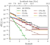 |
Fig. 3. Spectral energy density integrated over frequency for different redshift bins. The total contribution from all redshift bins is shown in black. Different colors indicate the contribution from different types of DWD binaries. |
However, it is interesting to note that at higher redshifts, CO-CO and ONe-CO binaries produce a higher SGWB than CO-He binaries. This is due to the typically long delays elapsing between the formation of their progenitor stellar binaries and that of the latter type DWDs. While CO-CO and ONe-CO binaries can be produced after only a few hundred million years of binary evolution (Istrate et al. 2014), the first CO-CO binaries take around ≲1 Gyr to form. Consequently, in the first few billion years after the onset of star formation, DWDs were mostly CO-CO and ONe-CO, which explains why they dominate the SGWB. The same argument applies to interpret the fact that the contribution of He-He binaries starts only after z ∼ 4. Indeed, stellar evolution and binary interactions prior to the formation of a He-He system typically extend over more than a billion years (see e.g., Lamberts et al. 2019).
On the other hand, the negligible contribution of ONe-ONe binaries manifest only at very low redshifts due to their typically high initial orbital separations that translate into extremely long evolution time to evolve up to the LISA frequency band. We show further results on the contribution of the different types of DWDs in Appendix A.3.
3.3. Including tidal effects and mass transfer during DWD evolution
We now explore the impact of interactions between DWDs, such as mass transfer and tidal interactions, on our predictions for the SGWB. In this subsection, we no longer use the simplified case to describe the orbital evolution of all DWDs through only GW emission, but evolve each system independently using the model of Toubiana et al. (2024), as described in 2.4.3, and recover more realistic descriptions of their complete evolution.
For all the DWDs formed at all metallicities in our default model, we simulated the complete temporal evolution of fe,  , and ℳc, starting from their initial orbital properties predicted by COSMIC at the instant of DWD formation. We injected these numerical expressions in Eq. (24) and computed the total fluxes received in each frequency bin using the standard SFRD from Madau & Dickinson (2014).
We show in Fig. 4 the SGWB from extragalactic DWDs obtained in the standard case assuming evolution through GW emission only (blue points), as well as the uncertainty in the energy density spectrum associated with uncertainties in the intensity of tidal effects (shaded blue area). We observe that the inclusion of DWD interactions modifies the SGWB energy density spectrum by a factor of ∼0.8 − 1.5 for supra-millihertz frequencies. This is because these interactions occur when the two WDs are close enough to each other. Toubiana et al. (2024) find that the typical GW frequency at which the out-spiraling systems accumulate is around 1.3 mHz. This roughly corresponds to the value of the observed GW frequency at which interactions start playing a noticeable role in our predictions of the SGWB. For the highest frequencies (fr ≥ 2 × 10⁻² Hz), the inclusion of tidal effects in the evolution of DWDs could increase their contribution to the SGWB by a factor of up to ∼3.
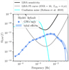 |
Fig. 4. SGWB from extragalactic DWDs when considering a more realistic treatment of DWD evolution, including episodes of mass transfer and tidal effects. The scatter points indicate the standard case with only GWs, with the default COSMIC model and SFRD from Madau & Dickinson (2014). The shaded area covers predictions from different assumptions about tidal effects. Additional curves represent the LISA sensitivity, the PI curve, and the confusion noise from Galactic DWDs. |
The lower estimate of the predicted SGWB corresponds to the model “low spins, weak tides” of Toubiana et al. (2024). Under these assumptions, some systems do not survive the first intense episode of mass transfer (see e.g., Pakmor et al. 2022), and the amplitude of the SGWB can then be slightly reduced compared to the simplified case of DWD evolution through GW emission alone. On the other hand, in the low spins, strong model tides of Toubiana et al. (2024) (upper edge of the shaded blue area) the tidal effects typically help to stabilize this first episode of mass transfer, and more systems survive. Under these assumptions, the amplitude of the SGWB is then pushed to slightly higher values in this frequency range due to the fact that some DWDs can contribute several times to the same frequency bin over the course of their evolution.
The inclusion of realistic interactions in the evolution of DWDs produces a noticeable impact on our predictions of the SGWB from these systems, but its effect appears to be less important than the model of cosmic star formation history or the treatment of the CE phase during the evolution of massive stellar binaries (see Fig. 1). For this reason, and in order to reduce the computational cost of our simulations, we have chosen not to include these realistic interactions in all the combinations of the different models used in this study. We believe, however, that it is important to bear in mind the contribution of these uncertainties for future analyses of the SGWB produced by extragalactic DWDs.
3.4. The presence of anisotropies in the SGWB from extragalactic DWDs
A practical exploration of anisotropies in the SGWB from extragalactic DWDs could theoretically be carried out by sampling sources across a realistic spatial distribution of galaxies inside a cosmological volume. However, this approach would require the production of large catalogs of sources and to considerably modify the code developed for this study. We propose here a complementary analysis that uses the procedure presented in this study to place upper limits on the relative importance of anisotropies in the SGWB from extragalactic DWDs.
In particular, we make the argument that if all the DWDs within a certain redshift range [0, zhomogeneous] contribute to X% of the total SGWB, and that the Universe is indeed homogeneous and isotropic beyond zhomogeneous, then at most X% of this GW signal can carry some signature of an anisotropic origin. We therefore consider the cumulative contribution of increasingly distant redshift shells to this SGWB as a tracer of the maximum impact that anisotropies in the distribution of galaxies could have on the GW signal.
Following Marinoni et al. (2012), we used a fiducial value of comoving distance 150 h−1 Mpc as the typical scale above which the Universe can be considered homogeneous and isotropic, which corresponds to a redshift of zhomogeneous ≃ 0.05 (Planck Collaboration VI 2020). We then split our initial first redshift bin in 20 new intervals between 0 and zhomogeneous and completed our discretization with the other redshift bins previously used. We show in Fig. 5 the cumulative contribution to the SGWB from extragalactic DWDs as a function of redshift over the complete frequency spectrum (black curve), and for different specific frequency bands (colored curves). The very low contribution of the z ≤ 0.05 Universe in most frequency bins suggests that the hypothesis of homogeneous and isotropic Universe applied to derive Eq. (7) remains valid, at least to a few percent.
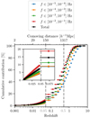 |
Fig. 5. Cumulative contribution of extragalactic DWDs to the SGWB as a function of redshift, using our default population synthesis model and the SFRD from Madau & Dickinson (2014). The black dots represent the integrated contribution over the complete frequency range, and the colored ones correspond to different specific frequency bands. The redshift marking the limit of the homogeneous isotropic Universe z = 0.05 is indicated as the vertical dashed gray line, as is z = 0.5. |
We find that the presence of anisotropies in the SGWB from extragalactic DWDs would represent a greater fraction at the highest frequencies, with around 10% of the signal in the range [10−2, 10−1] Hz originating from sources at z ≤ 0.05, against less than 5% in the range [10−5, 10−4] Hz. This fraction increases to ∼60% for sources in the range [10−2, 10−1] Hz at z ≤ 0.5, and ∼40% in the range [10−5, 10−4] Hz. As the distant systems emitting GWs at high frequencies have their signals redshifted to lower frequencies when observed on or near Earth, the range of high observed frequencies is naturally populated by close-by systems. This explains why the cumulative contribution is always higher in the observed frequency range [10−2, 10−1] Hz compared to the other frequency ranges, although it is less important in absolute energy density.
We remind the reader that the values indicated here represent the relative contribution to the total signal in each frequency band. Indeed, as the amplitude of the SGWB from extragalactic DWDs is predicted to be quite faint below 10−4 Hz and to drop rapidly above 10−2 Hz, LISA will most likely not be sensitive at all to the signal in these ranges of frequency (see Fig. 1). Looking specifically at the frequency range [10−3, 10−2] Hz, which corresponds to the region where LISA will be most sensitive and where the SGWB from extragalactic DWDs is predicted to be most important, we find that only ∼6% of the total signal would originate from sources located at z ≤ 0.05. Even if all the sources inside that volume were located at one unique position, their combined GW signal would still be completely dominated by the more distant sources in the rest of the Universe. Therefore, the results presented in Fig. 5 provide an upper limit on the maximal contribution of anisotropies to the total SGWB from extragalactic DWDs, as a function of the limit of the homogeneous and isotropic Universe one considers.
A similar analysis carried on with the alpha4 COSMIC model shows overall similar trends, although the contribution of the most distant sources appears to be slightly less important in the alpha4 model. This is because the DWDs formed through more efficient CE evolution typically have larger orbital separations when they form, and therefore take longer to evolve to the LISA frequency band, hence emitting at typically lower redshifts compared to the default model.
Considering additional sources of anisotropies in the GW signal from the modulated foreground, including contributions from sources in the Milky Way (Boileau et al. 2021; Bartolo et al. 2022) and in satellite galaxies (Roebber et al. 2020; Rieck et al. 2024), the presence of anisotropies in the SGWB from extragalactic DWDs becomes even more negligible. We conclude that the small amplitude of potential anisotropies in this SGWB will most likely not be observable by LISA.
4. Discussion
4.1. Uncertainties in modeling the SGWB
In this work we have explored the impact of different uncertainties on the spectrum and amplitude of the SGWB from extragalactic DWDs in the LISA band. First of all, our results are globally consistent with other recent studies (Farmer & Phinney 2003; Staelens & Nelemans 2024; Hofman & Nelemans 2024). The spectrum from Staelens & Nelemans (2024) lies in between two of our models, with different assumptions on the CE efficiency.
One notable difference between our predictions and those of Staelens & Nelemans (2024) and Hofman & Nelemans (2024) lies in the high-frequency part of the energy density spectrum. Indeed, while they find models for backgrounds that extend up to 10−2 Hz and start decreasing abruptly only for frequencies higher than ∼3 × 10⁻² Hz, all our models are already falling-off at frequencies around 7 × 10⁻³ Hz (see Fig. 1). Looking in detail at the properties of the sources that contribute in this frequency range, we find that they are for the vast majority massive DWDs with tight orbits (with typical values of ℳc ≥ 0.6 M⊙ and a ≤ 3 R⊙). The progenitors of these systems are stellar binaries formed with orbital separations already relatively low.
However, with our different COSMIC models, we barely manage to produce any of such massive and tight DWDs, even when evolving the exact same stellar progenitors as in Staelens & Nelemans (2024). Looking at the stellar evolution and various phases of binary interactions that are implemented within their code SeBa and within COSMIC, we were able to identify the main origin of the differences in the treatment of the CE evolution. Two factors play an important role here: first the criteria for the stability of mass transfer, which determines the stellar binaries that can evolve through stable mass transfer only until the formation of the two WDs, thus avoiding a potential merger during the CE phase; second the treatment of CE evolution itself.
In the version of the SeBa code used in Staelens & Nelemans (2024) and Hofman & Nelemans (2024), they used a criterion based on the binary angular momentum to determine the stability of mass transfer, whereas in COSMIC we used a criterion based on the mass ratio. In practice, this makes it so that less systems experience CE phases in SeBa and more of these massive stellar binaries survive to eventually produce DWDs. They also use a value of the binding energy factor of a star to its envelope to a constant value λ = 0.5. This helps the survivability of the most massive systems. These same massive systems typically merge during the CE phase in COSMIC, where we use a value of this binding energy factor that depends on stellar type (following Claeys et al. 2014).
To quantify the impact of these two different elements, we simulated two additional populations of DWDs with COSMIC, incorporating modifications to the alpha4 model. In the first model, we set the binding energy factor to λ = 0.5. In the second, we additionally modified the criterion for the stability of mass transfer inside COSMIC to mimic the one used in SeBa. The SGWB obtained for the standard default model, for the alpha4 one, and for these two additional models are shown in Fig. 6.
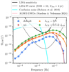 |
Fig. 6. SGWB from extragalactic DWDs with additional COSMIC models to mimic the different physical prescriptions applied in SeBa. The blue scatter points indicate the standard case, with our default COSMIC model and SFRD from Madau & Dickinson (2014). The red stars correspond to the alpha4 model. The orange ones correspond to the SGWB obtained when fixing in COSMIC the CE efficiency parameter to α = 4 and the binding energy factor of a star to its envelope to a constant value λ = 0.5. The green ones are obtained when using these same fixed values for α and λ, and modifying in COSMIC the criterion for mass transfer stability to resemble the one in SeBa. Additional curves represent the LISA sensitivity, the PI curve, and the confusion noise from Galactic DWDs. The pink curve indicates the best-fit model of the SGWB from extragalactic DWDs estimated in Staelens & Nelemans (2024). |
We observe a clear shift of the high-frequency part of the SGWB with these different prescriptions of CE evolution. The second model (green scatter points), which incorporates both the modification for the onset of unstable mass transfer and for the treatment of CE itself, gives results that are in much better agreement with the predictions presented in Staelens & Nelemans (2024) (pink curve) in the high-frequency regime. In particular, the location of the typical frequency at which the signal starts to drop, referred to here as the knee, increases toward higher frequencies in these two additional models where the evolution of the CE is treated in a similar way to SeBa.
The high-frequency regime will also be the most affected by tidal torques and/or mass transfer between the DWDs. Following the Toubiana et al. (2024) model, we find variation in amplitude by up to a factor of 2 at the highest frequencies. While the high-frequency regime appears to be the most interesting to study the effects of binary interaction, it is also the least likely to be detected, unless the signal amplitude is higher than predicted or the population of tight systems is more abundant than assumed. Given the high S/Ns predicted, it may possible to detect signatures of tidal interactions or mass transfer effects in the observed signal.
4.2. Implications of the knee frequency
Beyond the overall detectability of the SGWB from extragalactic DWDs, the knee frequency provides particularly valuable astrophysical information. This knee frequency is primarily determined by the existence of very massive DWDs with extremely low orbital separations. In addition to the natural scaling of orbital frequency with the mass of the binary components, white dwarfs have the particularity of seeing their radius decrease as their mass increases (see e.g., Kawaler 1997). This implies that more massive DWDs can reach smaller orbital separations before one starts filling its Roche lobe, hence increasing again the maximum frequency at which they can emit GWs before their merger. To contribute to the high-frequency part of the energy density power spectrum, these binaries must also exist at low redsfhits (otherwise their received frequency would be shifted to smaller values). The location of the frequency knee in the SGWB from extragalactic DWDs is therefore based on the possibility and efficiency of binary stellar evolution to produce two massive WDs very close to each other.
Models with more efficient envelope ejection (higher α or λ parameters) tend to produce wider post-CE separations, but also allow some binaries to survive the CE evolution phase, whereas they would merge during this phase in the case of less efficient energy transfer to the envelope. This explains why the SGWB from extragalactic DWDs predicted with our alpha4 COSMIC model extends to slightly higher frequencies than our default model (see Fig. 1 and Table B.1). This feature is explored in our comparison with the population synthesis code SeBa in the previous subsection (see e.g. the model λCE = 0.5 &  and the results of Staelens & Nelemans (2024) presented in Fig. 6).
Therefore, the precise location of this spectral break encodes direct constraints on CE physics, which remains one of the largest uncertainties in binary stellar evolution. Observing the knee frequency with LISA would thus offer an opportunity to constrain the physical prescriptions used for CE evolution and improve the predictions of population synthesis models. Future analyses should therefore focus on precise modeling and measurement of the knee frequency, together with the overall amplitude, to enhance our understanding of binary evolution physics using the SGWB from extragalactic DWDs observed by LISA.
5. Conclusions
In this study, we have presented new predictions for the SGWB produced by extragalactic DWDs, based on population synthesis models using COSMIC and three different SFRs. The amplitude and shape of the background strongly depend on key astrophysical assumptions, especially binary evolution physics and the SFR beyond redshift z ∼ 2.
Our main findings can be summarized as follows:
-
The signal is detectable by LISA across all scenarios explored, with S/Ns ranging from ∼100 to ∼400 for conservative models and exceeding ∼1000 for optimistic models (e.g., Strolger + alpha4). For 10-year integration, the S/N can reach up to ∼2400, indicating that the extragalatic DWD background will be robustly observed by LISA under all astrophysical assumption considered here.
-
The dominant uncertainty on ΩGW arises from the cosmic SFR (factor of ∼6 − 7), with additional variation from binary physics (factor of ∼2 − 3).
-
Tidal effects and post-formation mass transfer introduce a further modulation above 5 mHz, at the level of a factor of ∼2 − 3. These remain subdominant compared to population-wide assumptions.
-
Our findings are in line with previous studies in terms of amplitude of the signal, and power law behavior at low frequency. We confirm the variations based on the star formation model and binary evolution models.
-
A spectral break occurs around 7 mHz in our models, in contrast to earlier predictions near 20 mHz. This shift reflects differences in the formation and survival of compact, massive systems following mass transfer.
-
The signal is largely isotropic, with contributions from the nearby Universe (z < 0.05) at the percent level, insufficient for the detection of anisotropies.
Reducing model uncertainty requires improved treatment of binary evolution, particularly during the CE phase. Multi-messenger comparisons, such as those discussed in van Zeist et al. (2025), offer promising avenues to calibrate population synthesis outputs using electromagnetic constraints. Further cross-validation between independent codes (e.g., BPASS Stanway & Eldridge 2023; Byrne et al. 2025) will also help to identify robust features in SGWB predictions. Interpreting this detection will require careful modeling of foregrounds and explicit inclusion of the SGWB from extragalactic DWDs in future LISA data analysis pipelines. A more detailed analysis of its detectability and implications will be the subject of future works.
These results also underline that no reliable estimate of the detectability of cosmological SGWBs can be made without first accounting for the extragalactic DWD background. Its amplitude and spectral shape make it a dominant component in the LISA band. Accurate modeling of this signal is therefore essential to define the astrophysical foreground and to interpret any potential cosmological contribution. Ignoring it would lead to overly optimistic forecasts and biased conclusions (Boileau et al. 2021, 2022, 2023). The SGWB from extragalactic DWDs represents a dominant signal of SGWB in the LISA band and will severely limit the detectability of cosmological SGWBs. It must therefore be explicitly included in future simulations and in the data analysis pipelines developed within the LISA Science Ground Segment framework.
Acknowledgments
We sincerely thank the group of Gijs Nelemans for their valuable assistance and the constructive discussions that helped us better understand the differences between our results. We would also like to thank Arianna Renzini and Riccardo Buscicchio for their priceless comments and advice. Their insights were instrumental in refining our analysis and interpretations. G.B. thanks the Centre national d’études spatiales (CNES) for support for this research. This project has received financial support from the CNRS through the MITI interdisciplinary programs through its exploratory research program. A.L., T.B. and N.C. acknowledge support by the French Agence Nationale de la Recherche. T.B. and A.T. are supported by ERC Starting Grant No. 945155–GWmining, Cariplo Foundation Grant No. 2021-0555, MUR PRIN Grant No. 2022-Z9X4XS, MUR Grant “Progetto Dipartimenti di Eccellenza 2023–2027” (BiCoQ), and the ICSC National Research Centre funded by NextGenerationEU. A.T. is supported by MUR Young Researchers Grant No. SOE2024-0000125.
References
- Abbott, R., Abbott, T. D., Abraham, S., et al. 2021, Phys. Rev. D, 104 [Google Scholar]
- Abbott, R., Abbott, T. D., Acernese, F., et al. 2023, Phys. Rev. X, 13 [Google Scholar]
- Allen, B., & Romano, J. D. 1999, Phys. Rev. D, 59 [Google Scholar]
- Althaus, L. G., Córsico, A. H., Isern, J., & García-Berro, E. 2010, A&ARv, 18, 471 [NASA ADS] [CrossRef] [Google Scholar]
- Amaro-Seoane, P., Audley, H., Babak, S., et al. 2018, Liv. Rev. Relat., 21, 1 [Google Scholar]
- Auclair, P., Bacon, D., Baker, T., et al. 2023, Liv. Rev. Relat., 26, 5 [NASA ADS] [CrossRef] [Google Scholar]
- Babak, S., Hewitson, M.,& Petiteau, A. 2021, arXiv e-prints [arXiv:2108.01167] [Google Scholar]
- Bartolo, N., Bertacca, D., Caldwell, R., et al. 2022, ApJS, 2022, 009 [Google Scholar]
- Boileau, G., Lamberts, A., Christensen, N., Cornish, N. J., & Meyer, R. 2021, MNRAS, 508, 803 [Google Scholar]
- Boileau, G., Jenkins, A. C., Sakellariadou, M., Meyer, R., & Christensen, N. 2022, Phys. Rev. D, 105 [Google Scholar]
- Boileau, G., Christensen, N., Gowling, C., Hindmarsh, M., & Meyer, R. 2023, JCAP, 2023, 056 [Google Scholar]
- Breivik, K., Coughlin, S., Zevin, M., et al. 2020, ApJ, 898, 71 [Google Scholar]
- Buscicchio, R., Klein, A., Korol, V., et al. 2025, Eur. Phys. J. C, 85, 887 [Google Scholar]
- Byrne, C. M., Eldridge, J. J., & Stanway, E. R. 2025, MNRAS, 537, 2433 [Google Scholar]
- Caprini, C., & Figueroa, D. G. 2018, Class. Quantum Grav., 35 [Google Scholar]
- Caprini, C., Durrer, R., & Servant, G. 2009, ApJS, 2009, 024 [Google Scholar]
- Chen, Z.-C., Huang, F., & Huang, Q.-G. 2019, ApJ, 871, 97 [NASA ADS] [CrossRef] [Google Scholar]
- Christensen, N. 2018, Rep. Prog. Phys., 82 [Google Scholar]
- Claeys, J. S. W., Pols, O. R., Izzard, R. G., Vink, J., & Verbunt, F. W. M. 2014, A&A, 563, A83 [NASA ADS] [CrossRef] [EDP Sciences] [Google Scholar]
- Colpi, M., Danzmann, K., Hewitson, M., et al. 2024, arXiv e-prints [arXiv:2402.07571] [Google Scholar]
- Criswell, A. W., Rieck, S., & Mandic, V. 2025, Phys. Rev. D, 111 [Google Scholar]
- Eggleton, P. P. 1983, ApJ, 268, 368 [Google Scholar]
- Farmer, A. J., & Phinney, E. S. 2003, MNRAS, 346, 1197 [NASA ADS] [CrossRef] [Google Scholar]
- Goldberg, D., & Mazeh, T. 1994, A&A, 282, 801 [NASA ADS] [Google Scholar]
- Grevesse, N., & Sauval, A. J. 1998, SSRv, 85, 161 [NASA ADS] [Google Scholar]
- Hawking, S. W., & Israel, W. 1987, Three Hundred Years of (Gravitation (Cambridge University Press)) [Google Scholar]
- Hjellming, M. S., & Webbink, R. F. 1987, ApJ, 318, 794 [Google Scholar]
- Hofman, S., & Nelemans, G. 2024, A&A, 691, A261 [NASA ADS] [CrossRef] [EDP Sciences] [Google Scholar]
- Hurley, J. R., Tout, C. A., & Pols, O. R. 2002, MNRAS, 329, 897 [Google Scholar]
- Istrate, A. G., Tauris, T. M., Langer, N., & Antoniadis, J. 2014, A&A, 571, L3 [NASA ADS] [CrossRef] [EDP Sciences] [Google Scholar]
- Ivanova, N., Justham, S., Chen, X., et al. 2013, A&ARv, 21, 59 [Google Scholar]
- Karnesis, N., Babak, S., Pieroni, M., Cornish, N., & Littenberg, T. 2021, Phys. Rev. D, 104 [Google Scholar]
- Kawaler, S. D. 1997, White Dwarf Stars (Berlin (Heidelberg: Springer, Berlin Heidelberg)), 1 [Google Scholar]
- Kroupa, P. 2001, MNRAS, 322, 231 [NASA ADS] [CrossRef] [Google Scholar]
- Lamberts, A., Blunt, S., Littenberg, T. B., et al. 2019, MNRAS, 490, 5888 [NASA ADS] [CrossRef] [Google Scholar]
- Madau, P., & Dickinson, M. 2014, ARA&A, 52, 415 [Google Scholar]
- Madau, P., & Fragos, T. 2017, ApJ, 840, 39 [Google Scholar]
- Marinoni, C., Bel, J., & Buzzi, A. 2012, ApJS, 2012, 036 [Google Scholar]
- Mazumdar, A., & White, G. 2019, Rep. Prog. Phys., 82 [Google Scholar]
- Moe, M., & Di Stefano, R. 2017, ApJS, 230, 15 [Google Scholar]
- Neijssel, C. J., Vigna-Gómez, A., Stevenson, S., et al. 2019, MNRAS, 490, 3740 [Google Scholar]
- Nelemans, G., Yungelson, L. R., Portegies Zwart, S. F., & Verbunt, F. 2001, A&A, 365, 491 [NASA ADS] [CrossRef] [EDP Sciences] [Google Scholar]
- Nissanke, S., Vallisneri, M., Nelemans, G., & Prince, T. A. 2012, ApJ, 758, 131 [NASA ADS] [CrossRef] [Google Scholar]
- Pakmor, R., Callan, F. P., Collins, C. E., et al. 2022, MNRAS, 517, 5260 [NASA ADS] [CrossRef] [Google Scholar]
- Phinney, E. S. 2001, MNRAS, submitted [arXiv:astroph/0108028] [Google Scholar]
- Planck Collaboration VI. 2020, A&A, 641, A6 [NASA ADS] [CrossRef] [EDP Sciences] [Google Scholar]
- Portegies Zwart, S. F., & Verbunt, F. 1996, A&A, 309, 179 [NASA ADS] [Google Scholar]
- Pozzoli, F., Buscicchio, R., Klein, A., et al. 2025, Phys. Rev. D, 111 [Google Scholar]
- Price-Whelan, A. M., Lim, P. L., Earl, N., et al. 2022, ApJ, 935, 167 [NASA ADS] [CrossRef] [Google Scholar]
- Regimbau, T., & Mandic, V. 2008, Class. Quant. Grav., 25 [Google Scholar]
- Rieck, S., Criswell, A. W., Korol, V., et al. 2024, MNRAS, 531, 2642 [Google Scholar]
- Robitaille, T. P., Tollerud, E. J., Greenfield, P., et al. 2013, A&A, 558, A33 [NASA ADS] [CrossRef] [EDP Sciences] [Google Scholar]
- Robson, T., Cornish, N. J., & Liu, C. 2019, Class. Quant. Grav., 36 [Google Scholar]
- Roebber, E., Buscicchio, R., Vecchio, A., et al. 2020, ApJ, 894, L15 [NASA ADS] [CrossRef] [Google Scholar]
- Sana, H., de Mink, S. E., de Koter, A., et al. 2012, Science, 337, 444 [Google Scholar]
- Schneider, R., Ferrari, V., Matarrese, S., & Portegies Zwart, S. F. 2001, MNRAS, 324, 797 [NASA ADS] [CrossRef] [Google Scholar]
- Smith, T. L., & Caldwell, R. R. 2019, Phys. Rev. D, 100 [Google Scholar]
- Speagle, J. S. 2020, MNRAS, 493, 3132 [Google Scholar]
- Staelens, S., & Nelemans, G. 2024, A&A, 683, A139 [NASA ADS] [CrossRef] [EDP Sciences] [Google Scholar]
- Stanway, E. R., & Eldridge, J. J. 2023, MNRAS, 522, 4430 [NASA ADS] [CrossRef] [Google Scholar]
- Strolger, L.-G., Riess, A. G., Dahlen, T., et al. 2004, ApJ, 613, 200 [Google Scholar]
- Thorpe, J. I., Ziemer, J., Thorpe, I., et al. 2019, BAAS, 51, 77 [NASA ADS] [Google Scholar]
- Thrane, E., & Romano, J. D. 2013, Phys. Rev. D, 88 [Google Scholar]
- Tinto, M., Estabrook, F. B., & Armstrong, J. W. 2004, Phys. Rev. D, 69 [Google Scholar]
- Toonen, S., Nelemans, G., & Portegies Zwart, S. 2012, A&A, 546, A70 [NASA ADS] [CrossRef] [EDP Sciences] [Google Scholar]
- Toubiana, A., Karnesis, N., Lamberts, A., & Miller, M. C. 2024, A&A, 692, A165 [NASA ADS] [CrossRef] [EDP Sciences] [Google Scholar]
- Ungarelli, C., & Vecchio, A. 2001, Phys. Rev. D, 64 [Google Scholar]
- van Haaften, L. M., Nelemans, G., Voss, R., et al. 2013, A&A, 552, A69 [NASA ADS] [CrossRef] [EDP Sciences] [Google Scholar]
- van Zeist, W. G., van Roestel, J., Nelemans, G., et al. 2025, A&A, 699, A172 [NASA ADS] [CrossRef] [EDP Sciences] [Google Scholar]
- Vink, J. S., & de Koter, A. 2005, A&A, 442, 587 [NASA ADS] [CrossRef] [EDP Sciences] [Google Scholar]
- Vink, J. S., de Koter, A., & Lamers, H. J. G. L. M. 2001, A&A, 369, 574 [NASA ADS] [CrossRef] [EDP Sciences] [Google Scholar]
Appendix A: Comparison with previous studies
Here we present numbers and plots to enable a direct comparison with Staelens & Nelemans (2024), and provide additional figures detailing the contributions of different types of DWDs.
A.1. Physical properties of DWDs at formation and formation efficiency
Fig. A.1 shows the distribution of orbital frequencies at the instant of formation for the DWDs obtained with our default COSMIC model. CO-CO pairs form from originally wide stellar binaries that do not undergo envelope stripping before He begins to burn in the core, and generally result in wide DWD systems with therefore fairly low orbital frequencies. He-He pairs, on the other hand, come from two lower mass stars in a tight binary where the two stars have had their envelopes removed by binary interactions at some point in their evolution. This results in DWD systems with typically higher initial orbital frequencies. CO-He systems are formed through a combination of these two phenomena. The systems containing at least one ONe WD originate from more massive stars and are naturally less common. As only the widest of these massive binaries can evolve without undergoing stellar mergers, ONe-ONe pairs are typically formed with large orbital separations, meaning low initial orbital frequencies, and most of these systems emit so few GWs that they will never actually enter the LISA band.
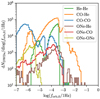 |
Fig. A.1. Distribution of orbital frequencies at the instant of formation forb, 0 of the DWDs produced with our default COSMIC model at solar metallicity. This set of DWDs contains only those that have passed the low-frequency cutoff and could potentially end up in the LISA band. Each colored curve represents a specific type of DWD. |
Fig. A.2 presents the distribution of all DWD systems at formation in the parameter space (fe, 0,ℳc), where fe, 0 is the emission frequency of GWs at the instant of DWD formation and ℳc is the chirp mass. This figure can be directly compared with Figure 1 in Staelens & Nelemans (2024). As the first three models default, fb1, and multidim, use the exact same physics to describe binary evolution but differ only in the properties of their initial stellar populations, they predict DWD systems with overall similar masses and orbital properties. On the other hand, the COSMIC model α4 with a higher CE efficiency parameter results in a population of DWDs with typically smaller GW frequencies at formation. The peak of the distribution lies around fe, 0 ≲ 10−3 Hz and ℳc ∼ 0.3 M⊙, which correspond to the typical masses and frequencies at which CO-He and He-He pairs are formed (see Fig. A.1).
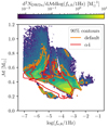 |
Fig. A.2. Density plot of the chirp mass ℳc and GW frequency at the time of formation fe, 0 of all the DWDs produced by our default COSMIC model at solar metallicity (color map). Solid lines show the contours containing 90% of the DWDs in the parameter space (fe, 0, ℳc) for this default model (orange) as well as for the alpha4 model (red). |
In order to consistently compare DWD formation across our different COSMIC models, we consider the DWD formation efficiency defined as
 (A.1)
(A.1)
where NDWDs(Z) is the number of DWDs formed from the evolution of the stellar population initialized with metallicity Z, and MSF(Z) is the total initial mass of the stellar population, including both single and binary stars. We show in Fig. A.3 the evolution of this DWD formation efficiency η as a function of metallicity for our four COSMIC models. As WDs stem from only moderately massive stars, where mass loss through stellar winds is less important, the impact of metallicity on the formation of DWDs is expected to be only a minor effect. We observe that for all models, there is a factor of at most ∼1.5 between η(0.01Z⊙) and η(Z⊙), which confirms the moderate influence of metallicity on DWD formation. The default model is consistently the least efficient in forming DWDs, whereas the models fb = 1 and multidim agree for the most part across all metallicities. The model α4 predicts a DWD formation efficiency roughly 3 times that of the other three models, and shows no clear sign of decreasing with metallicity.
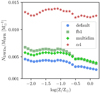 |
Fig. A.3. Formation efficiency of DWDs as a function of metallicity for the four COSMIC models considered in this study. At each metallicity, η was computed as the number of DWD sytems formed above the low-frequency cutoff divided by the total mass of the stellar population simulated in COSMIC. |
A.2. Metallicity-dependent star formation history
Best-fit parameters of the three different SFRD models considered in this study.
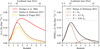 |
Fig. A.4. Left: SFRD in the Universe as a function of redshift. Different colors indicate different estimates based on different assumptions on the IMF of stellar populations or on extinction correction (Strolger et al. 2004; Madau & Dickinson 2014; Madau & Fragos 2017). Right: Metallicity-specific SFRD as a function of redshift for different values of metallicity, computed as the combination of the SFRD from Madau & Dickinson (2014) with the metallicity distribution of Neijssel et al. (2019). The dashed, dot-dashed, and dotted lines show the metallicity-specific SFRD around metallicity Z⊙, 0.1 × Z⊙, and 0.01 × Z⊙ respectively. |
The left-hand panel of Fig. A.4 shows the SFRDs according to these three different models in this paper. They all agree reasonably well at low redshifts (z ≲ 2) but the model from Strolger et al. (2004) finds substantially more star formation at higher redshifts. The right-hand panel of Fig. A.4 shows the results of the combination of the SFRD from Madau & Dickinson (2014) with the metallicity distribution function of Neijssel et al. (2019). Under these assumptions, most of star formation takes place at z ≤ 2 and involves already metal-enriched stars (at Z ∼ Z⊙), while the formation of stars at Z ∼ 0.1 Z⊙ principally takes place at around z ∼ 5. The most metal-poor stars at Z ∼ 0.01 Z⊙ are rare and form almost exclusively at the highest redshifts (z ≲ 8).
A.3. Progenitor metallicity of the DWDs contributing to the SGWB
Fig. A.5 presents the energy density spectrum for the different types of DWDs as a function of progenitor metallicity, using our default COSMIC model and the SFRD from Madau & Dickinson (2014). We show here only the contributions to the SGWB for stellar progenitors formed at metallicities at Z⊙ (dashed lines), 0.1 × Z⊙ (dash-dotted lines), and 0.01 × Z⊙ (dotted lines), but the total energy density spectrum, plotted as solid lines, are still estimated for all the systems formed in our COSMIC model from the 25 different metallicities simulated. For all types of DWDs, with the exception of ONe-ONe binaries whose total contribution is negligible at all frequencies, the SGWB is dominated by systems formed through the evolution of binaries around Z⊙. This is directly inherited from our model of the metallicity-specific SFRD (see Eq. 15), which predicts that most of star formation takes place at redshift z ∼ 2 in environments where the metallicity is already close to the solar value (see Fig. A.4). Although systems formed at higher redshifts from metal-poor stellar progenitors may have more time to evolve and eventually enter the LISA frequency band, there are just not enough of them due to the limited star formation at these redshifts.
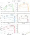 |
Fig. A.5. SGWB from extragalactic DWDs for the various types of DWDs and for different metallicities of stellar progenitors. In each sub-figure, the solid colored line shows the energy density spectrum of the total SGWB from this type of DWD while the dashed, dash-dotted, and dotted lines show the contribution of DWDs formed by the evolution of stellar progenitors around metallicity Z⊙, 0.1 × Z⊙, and 0.01 × Z⊙ respectively. Colored lines indicate the contributions from different DWD types. The plot highlights the overall SGWB with different line styles for each type of DWD binary: CO-CO binaries are shown in blue, CO-He binaries in orange, He-He binaries in green, ONe-CO binaries in red, ONe-He binaries in brown, and ONe-ONe binaries in olive. |
Appendix B: Estimating the SGWB using a smoothly broken power law fit
This appendix gathers the results of the SGWB energy spectral density summarize on Fig. 1. We investigate whether the SGWB from extragalactic DWDs can be effectively modeled by a simple analytical expression. For that, we adopt a smoothly broken power-law function and assess how well it fits our simulated SGWB across astrophysical synthesis scenarios or hypotheses. This model is motivated by the physical properties of the DWD population contributing to the SGWB from extragalactic DWDs. At low frequencies, the background follows a power-law behavior characteristic of a superposition of binary inspirals. However, the finite size and physical constraints of white dwarfs prevent them from emitting efficiently at high frequencies, leading to a depletion of sources and thus a spectral turnover. This transition defines a break in the spectrum. The break is smooth rather than abrupt, as the underlying binary population exhibits a distribution of physical parameters such as masses and orbital separations.
We fit a smoothly broken power-law model to estimate the SGWB from extragalactic DWDs across the different scenarios of SFRD and initial population parameters introduced in this paper. The model is defined as follows:
![Mathematical equation: $$ \begin{aligned} \Omega _{\text{ Model}}(f) = A \left( \frac{f}{f_b} \right) ^ {-\alpha _1} \left\{ \frac{1}{2} \left[1 + \left( \frac{f}{f_b}\right)^{1 / \Delta }\right]\right\} ^{(\alpha _1 - \alpha _2) \Delta } , \end{aligned} $$](/articles/aa/full_html/2025/10/aa56052-25/aa56052-25-eq40.gif) (B.1)
(B.1)
where A is the amplitude, fb is the frequency location of the knee, α1 and α2 are the spectral indices before and after this frequency, and δ controls the smoothness of the transition. The implementation of this model was facilitated using the smoothly broken power law from the astropy library (Robitaille et al. 2013); astropy:2022.
In our analysis, the spectral fitting of the SGWB from extragalactic DWDs is carried out using the dynesty library (Speagle 2020), which implements a nested-sampling Markov chain Monte Carlo (MCMC) algorithm. This Bayesian approach yields posterior distributions for the model parameters, their uncertainties, and the model evidence for possible comparison. The likelihood is defined as the sum of squared differences between the model and the simulated SGWB from extragalactic DWDs spectrum, weighted by the standard deviation of data accross the fit region.
This methodology follows closely the approach developed in previous studies of the SGWB for LISA, which employed similar MCMC-based strategies for spectral parameter estimation (Boileau et al. 2021, 2022). In particular, Boileau et al. (2021) introduced an adaptive MCMC algorithm to analyze simulated LISA data, demonstrating the effectiveness of Bayesian inference in separating astrophysical and cosmological background components. Building on this, Boileau et al. (2022) extended the Bayesian MCMC framework to assess the detectability of a cosmologically generated background in the presence of a foreground, highlighting the relevance of such techniques for SGWB analyses. By adopting a nested-sampling MCMC approach in this work, we ensure methodological continuity with these studies, which strengthens the reliability of our SGWB from extragalactic DWDs spectral estimation and enables direct comparison with previous results in the LISA context.
The parameters of the fit for each SFRD and initial population case are summarized in Table B.1, and we show a comparison between the fit and the true signal for the default model in Fig. B.1. For each fit, we initialize a range of plausible parameters informed by the physical constraints of the SGWB from extragalactic DWDs. The nested sampling approach ensured accurate estimation of posterior distributions.
Fit parameters for different initial populations.
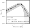 |
Fig. B.1. Total GW background spectrum computed using the default model for the DWD population and the Madau & Dickinson star formation history. The solid line represents the fit, and the shaded area indicates the 1σ uncertainty region. |
All Tables
Best-fit parameters of the three different SFRD models considered in this study.
All Figures
|
Fig. 1. Spectral energy density of the SGWB from extragalactic DWDs for various population synthesis models (see Sect. 2.3) and various SFRD models (see Sect. 2.4.1). The different population synthesis models are indicated with the same markers as in Fig. A.3. Dotted, solid, and dashed lines correspond to the SFR models from Strolger et al. (2004), Madau & Dickinson (2014), and Madau & Fragos (2017) respectively. The black line represents the LISA sensitivity curve (Colpi et al. 2024), while the gray one shows the PI curve (Thrane & Romano 2013) for four years of observation time and S/N = 10. The light blue curve is the confusion noise from Galactic DWDs (Robson et al. 2019) and the green green band is the 90% credible interval of the SGWB from all compact object binaries estimated from observations of GWs (Abbott et al. 2023). As a comparison, the shaded blue band shows the SGWB from extragalactic DWDs estimated in (Farmer & Phinney 2003) and the pink curve indicates the best-fit model obtained in (Staelens & Nelemans 2024). In Appendix B, we discuss and summarize the fits of SGWB from extragalactic DWDs of all SFR models and stellar population synthesis models as presented in Table B.1. |
| In the text | |
|
Fig. 2. Spectral energy density of the SGWB from extragalactic DWDs for the various types of DWDs, with our default COSMIC model and the SFRD from Madau & Dickinson (2014). Different colors indicate the contribution from different type of DWD binaries. We do not show the contribution of ONe-ONe binaries here, as it is several orders of magnitude below due to their rarity. The sum of all the contributions is shown in black. Additional curves represent the LISA sensitivity, the PI curve, and the confusion noise from Galactic DWDs. |
| In the text | |
|
Fig. 3. Spectral energy density integrated over frequency for different redshift bins. The total contribution from all redshift bins is shown in black. Different colors indicate the contribution from different types of DWD binaries. |
| In the text | |
|
Fig. 4. SGWB from extragalactic DWDs when considering a more realistic treatment of DWD evolution, including episodes of mass transfer and tidal effects. The scatter points indicate the standard case with only GWs, with the default COSMIC model and SFRD from Madau & Dickinson (2014). The shaded area covers predictions from different assumptions about tidal effects. Additional curves represent the LISA sensitivity, the PI curve, and the confusion noise from Galactic DWDs. |
| In the text | |
|
Fig. 5. Cumulative contribution of extragalactic DWDs to the SGWB as a function of redshift, using our default population synthesis model and the SFRD from Madau & Dickinson (2014). The black dots represent the integrated contribution over the complete frequency range, and the colored ones correspond to different specific frequency bands. The redshift marking the limit of the homogeneous isotropic Universe z = 0.05 is indicated as the vertical dashed gray line, as is z = 0.5. |
| In the text | |
|
Fig. 6. SGWB from extragalactic DWDs with additional COSMIC models to mimic the different physical prescriptions applied in SeBa. The blue scatter points indicate the standard case, with our default COSMIC model and SFRD from Madau & Dickinson (2014). The red stars correspond to the alpha4 model. The orange ones correspond to the SGWB obtained when fixing in COSMIC the CE efficiency parameter to α = 4 and the binding energy factor of a star to its envelope to a constant value λ = 0.5. The green ones are obtained when using these same fixed values for α and λ, and modifying in COSMIC the criterion for mass transfer stability to resemble the one in SeBa. Additional curves represent the LISA sensitivity, the PI curve, and the confusion noise from Galactic DWDs. The pink curve indicates the best-fit model of the SGWB from extragalactic DWDs estimated in Staelens & Nelemans (2024). |
| In the text | |
|
Fig. A.1. Distribution of orbital frequencies at the instant of formation forb, 0 of the DWDs produced with our default COSMIC model at solar metallicity. This set of DWDs contains only those that have passed the low-frequency cutoff and could potentially end up in the LISA band. Each colored curve represents a specific type of DWD. |
| In the text | |
|
Fig. A.2. Density plot of the chirp mass ℳc and GW frequency at the time of formation fe, 0 of all the DWDs produced by our default COSMIC model at solar metallicity (color map). Solid lines show the contours containing 90% of the DWDs in the parameter space (fe, 0, ℳc) for this default model (orange) as well as for the alpha4 model (red). |
| In the text | |
|
Fig. A.3. Formation efficiency of DWDs as a function of metallicity for the four COSMIC models considered in this study. At each metallicity, η was computed as the number of DWD sytems formed above the low-frequency cutoff divided by the total mass of the stellar population simulated in COSMIC. |
| In the text | |
|
Fig. A.4. Left: SFRD in the Universe as a function of redshift. Different colors indicate different estimates based on different assumptions on the IMF of stellar populations or on extinction correction (Strolger et al. 2004; Madau & Dickinson 2014; Madau & Fragos 2017). Right: Metallicity-specific SFRD as a function of redshift for different values of metallicity, computed as the combination of the SFRD from Madau & Dickinson (2014) with the metallicity distribution of Neijssel et al. (2019). The dashed, dot-dashed, and dotted lines show the metallicity-specific SFRD around metallicity Z⊙, 0.1 × Z⊙, and 0.01 × Z⊙ respectively. |
| In the text | |
|
Fig. A.5. SGWB from extragalactic DWDs for the various types of DWDs and for different metallicities of stellar progenitors. In each sub-figure, the solid colored line shows the energy density spectrum of the total SGWB from this type of DWD while the dashed, dash-dotted, and dotted lines show the contribution of DWDs formed by the evolution of stellar progenitors around metallicity Z⊙, 0.1 × Z⊙, and 0.01 × Z⊙ respectively. Colored lines indicate the contributions from different DWD types. The plot highlights the overall SGWB with different line styles for each type of DWD binary: CO-CO binaries are shown in blue, CO-He binaries in orange, He-He binaries in green, ONe-CO binaries in red, ONe-He binaries in brown, and ONe-ONe binaries in olive. |
| In the text | |
|
Fig. B.1. Total GW background spectrum computed using the default model for the DWD population and the Madau & Dickinson star formation history. The solid line represents the fit, and the shaded area indicates the 1σ uncertainty region. |
| In the text | |
Current usage metrics show cumulative count of Article Views (full-text article views including HTML views, PDF and ePub downloads, according to the available data) and Abstracts Views on Vision4Press platform.
Data correspond to usage on the plateform after 2015. The current usage metrics is available 48-96 hours after online publication and is updated daily on week days.
Initial download of the metrics may take a while.