| Issue |
A&A
Volume 702, October 2025
|
|
|---|---|---|
| Article Number | A19 | |
| Number of page(s) | 11 | |
| Section | Stellar atmospheres | |
| DOI | https://doi.org/10.1051/0004-6361/202556306 | |
| Published online | 01 October 2025 | |
Stable magnetic fields and changing starspots on Vega
An ultra-deep decadal survey at Pic du Midi and OHP
1
Université de Toulouse; UPS-OMP; IRAP ;
Toulouse,
France
2
CNRS; IRAP ;
14, avenue Edouard Belin,
31400
Toulouse,
France
3
Observatoire Midi-Pyrénées,
14 ave Edouard Belin,
31400
Toulouse,
France
4
Institut für Mathematik, Universität Potsdam,
14476
Potsdam,
Germany
5
Tartu Observatory, University of Tartu,
Observatooriumi 1,
Tõravere
61602,
Estonia
6
INAF – Osservatorio Astronomico di Brera,
via E. Bianchi 46,
23807
Merate,
Italy
★ Corresponding author: This email address is being protected from spambots. You need JavaScript enabled to view it.
Received:
8
July
2025
Accepted:
13
August
2025
Abstract
Aims. Monitoring magnetic and activity variations in A and B stars with ultra-weak magnetic fields is essential to our understanding of the origin and evolution of these fields in this domain of the Hertzsprung-Russell (HR) diagram. Vega is a prototype star of its type and its long-term monitoring offers the most promising opportunity to study these properties.
Methods. High-resolution spectrocopic and spectropolarimetric data were gathered with SOPHIE/OHP in 2018 and NARVAL/NEO-NARVAL/TBL in 2018, 2023, and 2024. A total of 13 108 individual spectra of Vega were obtained, which are the basis for the analysis carried out in this work. Magnetic field maps were reconstructed with the Zeeman-Doppler imaging (ZDI) method, while activity maps were reconstructed with an innovative code built for this purpose. These maps were compared to previous results.
Results. The rotation period of Vega was confirmed to be very close to the former reference period of 0.678 d. The average magnetic field confirms a negative spot of radial field on the pole with stable strength, while the magnetic maps confirm the long-term stability of an oblique dipole, as well as smaller magnetic features showing up consistently throughout our three observing epochs. However, brightness maps show strong variations of the spot location over a timescale of years (and possibly even shorter). The spot contrast is shown to be very similar in the observations from 2012, 2018, 2023, and 2024, with a normalised spectral amplitude of 0.0003. A direct correlation between the magnetic field and brightness patches could not be revealed in the simultaneous SOPHIE and NARVAL 2018 dataset.
Conclusions. Vega’s so-called magnetic mystery has gained complexity since indications point towards the presence of a fossil magnetic field, but also to the presence of a dynamo-generated field, most likely concentrated on equatorial regions.
Key words: stars: early-type / stars: magnetic field / stars: individual: Vega / stars: rotation
© The Authors 2025
 Open Access article, published by EDP Sciences, under the terms of the Creative Commons Attribution License (https://creativecommons.org/licenses/by/4.0), which permits unrestricted use, distribution, and reproduction in any medium, provided the original work is properly cited.
This article is published in open access under the Subscribe to Open model. This email address is being protected from spambots. You need JavaScript enabled to view it. to support open access publication.
1 Introduction
In 2009, the first important discovery of a weak magnetic field in a normal A-type star (Vega, −0.6 ± 0.3 G for the disk-averaged line-of-sight component) was announced by Lignières et al. (2009). Since then, this prototype star has been studied extensively in spectroscopy, velocimetry, and spectropolarimetry. Vega’s characteristics and physical parameters are described in detail in Böhm et al. (2015). The most important properties for the purposes of this work include the recently redetermined quasi-pole-on vision of i = 6.4 ± 0.5°, a v sin i = 21.6 ± 0.3 km s−1, and an equatorial velocity of veq = 195 ± 15 km s−1, based on an in-depth Fourier analysis of Vega’s spectral line profiles (Takeda 2021).
Observations over five nights with SOPHIE/OHP in 2012 led Böhm et al. (2015) to the major discovery and unambiguous confirmation of a structured stellar surface at very faint amplitude levels in the dynamical spectra of ΔF/Fc ~ 5 × 10⁻⁴ (with Fc being the continuum flux) corotating with the star. This is the first strong piece of evidence that standard A-type stars can show surface structures, opening up a new field of research. In particular, questions have arisen regarding a potential link with the recently discovered weak magnetic field discoveries in this category of stars.
Petit et al. (2017) used the same dataset to reconstruct Doppler imaging maps of the star. Their maps, corresponding to different nights, are mostly coherent, with apparent changes possibly due to the residual noise. In addition, marginal indications were found for a differential rotation of Vega, with the pole and the equator rotating at higher rates than the intermediate latitude regions. Nonetheless, the overall spectroscopic magnetic field signature (averaged circularly polarised line profiles) and derived surface magnetic maps for the different epochs between 2008 and 2018 remained very similar, showing a striking magnetic stability of Vega over one decade (Petit et al. 2022).
Following the first discovery of a magnetic field in Vega in 2009, similar fields were detected in other bright Am stars (Petit et al. 2011; Blazère et al. 2016). The idea therefore gained support that very weak magnetic fields are present in many A and B type stars. A rotational modulation linked to the presence of starspots might have been revealed in intermediate-mass stars lacking strong magnetic fields in the observations relying on Kepler photometry (Balona 2017; Balona 2019).
These results are of major importance for our knowledge of the evolution of intermediate-mass stars. Previously, this category of stars with radiative outer layers was not expected to display magnetic field generation. In contrast to lower mass stars with developed subphotospheric convection zones, such as our Sun, no mechanism of magnetic field and associated stellar surface structure generation has yet been established for this type of standard A-type star. Proposed scenarios include either decaying weak fossil field (Braithwaite & Cantiello 2013), dynamo fields constantly regenerated either in the thin He II convective layer (Cantiello & Braithwaite 2019) or in the differentially rotating radiative envelope through Tayler (Spruit 2002; Petitdemange et al. 2024), or magneto-rotational instabilities (Meduri et al. 2024).
Studying Vega as a prototype star extensively via spectropolarimetric observations will offer a first understanding of the nature of the magnetic field (i.e. fossil and/or dynamo, or a combination of both). A varying magnetic field in Vega would suggest that a dynamo process is at work in the envelope of intermediate-mass stars. At this stage, we have not established an observational method of differentiating between the various amplification mechanisms that are possibly involved in a dynamo.
A direct comparison of successive magnetic field maps produced by the Zeeman-Doppler imaging (ZDI) tomographic method, as well as spot maps produced in unpolarised light by Doppler imaging or similar reconstruction techniques, enables us to constrain the origin and properties of the magnetic field. This approach helps unveil possible temporal changes related to dynamo action. Beyond the question of intermediate-mass magnetism, the Vega Doppler maps also provide the first detailed constraints on the flow structure at the surface of a stellar radiative envelope.
This work is organised as follows. Section 2 presents the observations and data reduction. Section 3 presents the spectropolarimetric results. Section 4 presents the analysis of the activity tracing starspots present in the different datasets. Finally, we present a discussion and our conclusions in Sect. 5.
Log of the spectroscopic and spectropolarimetric observations of Vega.
2 Observations and data reduction
Table 1 summarises the high-resolution observations analyzed in this study. In 2018, Vega was observed simultaneously in spectropolarimetry with NARVAL (TBL/Pic du Midi, France, Aurière 2003) and SOPHIE/OHP (Perruchot et al. 2008, Bouchy et al. 2013). The goal was to combine stellar magnetic field observations with intensity observations obtained with an instrument stabilised in terms of velocimetry, with the intrinsic radial velocity variations of SOPHIE being lower than 2–3 ms−1. While NARVAL acquired spectra in polarimetric mode at R = 65 000, SOPHIE was used in its high-resolution mode (R = 75 000). The polarimetric results obtained with NARVAL in 2018 were already included in a first publication (Petit et al. 2022), while the intensity profiles were not exploitable at that time due to data reduction issues of the former pipeline. This issue is resolved in this paper thanks to our new data reduction software, described below. In 2019, NARVAL was upgraded to the highly stabilised spectropolarimeter-velocimeter NEO-NARVAL (Böhm et al. 2016). The 2023 and 2024 dataset observed with NEO-NARVAL suffered from poor weather conditions and a slightly less efficient instrument, basically due to a loss of blue flux. Table 1 shows a total of 13108 individual spectra of Vega obtained and analyzed in this article. Additional archival data from our 2012 observing run was used, described in detail in Böhm et al. (2015).
For each run, the observing strategy was to obtain as many well exposed Vega spectra during the whole night as possible in a continuous way, with all allocated nights as closely spaced as possible (i.e. in the best case, five to seven consecutive nights). Vega has a rotation period of ![Mathematical equation: $\[0.678_{-0.029}^{+0.036}\]$](/articles/aa/full_html/2025/10/aa56306-25/aa56306-25-eq1.png) d, detected in spectropolarimetric magnetic field observations by Alina et al. (2012) and confirmed in surface intensity observations by Böhm et al. (2015). This short rotation period enables complete and dense rotational phase coverage with the presented observing strategy.
d, detected in spectropolarimetric magnetic field observations by Alina et al. (2012) and confirmed in surface intensity observations by Böhm et al. (2015). This short rotation period enables complete and dense rotational phase coverage with the presented observing strategy.
The data reduction of the SOPHIE dataset was done with the SOPHIE Data Reduction Software (Bouchy et al. 2009). The NARVAL and NEO-NARVAL datasets were reduced with the NEXTRA Data Reduction Software (Böhm & Holschneider, in prep.) for homogeneity. An alternative reduction of the NARVAL data with Libre-Esprit by Donati et al. (1997) was also used for comparison to ensure the quality of the NEXTRA data reduction. The NEXTRA pipeline implements the flat-relative optimal extraction algorithm of Zechmeister et al. (2014) and produces Stokes I (intensity) and Stokes V (circular polarisation) spectra, based on the combination of four polarimetric sub-exposures. All resulting spectra were normalised to the local continuum by a dedicated normalisation routine within NEXTRA based on B-spline-fitting of each order at selected wavelength positions, each star requiring an individual pointing file fixing continuum zones. The spectra were also set in the barycentric velocity frame making use of the python library barycorrpy (Kanodia & Wright 2018).
The next step consisted of the extraction of least-square deconvolved (LSD) equivalent Stokes I (unpolarised) and Stokes V (circularly polarised) photospheric line profiles (Donati et al. 1997; Kochukhov et al. 2010) for all spectra. The underlying idea of the LSD technique is to make use of the multiplex information of hundreds to thousands of spectral lines in order to produce a common, very high signal-to-noise ratio (S/N) equivalent photospheric line profile. This applies also for LSD Stokes V profiles, taking into account the effective Landé factor of each line revealing the sensitivity of the line to magnetic fields. An atomic data linelist was used with Teff = 10 000 K and log g = 4.0, yielding a spectral line mask corresponding to Vega’s polar temperature and surface gravity using solar abundances. Eventually, only 207 spectral lines were retained using the interactive tool SpecpolFlow (Erba 2024; Folsom et al. 2025), based on the best fitting of mostly unblended spectral lines in normalised continuum zones excluding hydrogen lines, ‘flat-bottomed’ lines (for details, see Takeda et al. 2008), and telluric line areas. This preparation was crucial for obtaining high-S/N LSD profiles for Stokes I and Stokes V using LSDpy1. The velocity sampling was adapted to the slightly different resolution of SOPHIE and NEO-NARVAL (SOPHIE: 1.7 km s−1 versus NEO-NARVAL: 2.3 km s−1). Theoretically implementing a super-resolved oblique PSF extraction could mitigate the larger pixel size (see e.g. Piskunov et al. 2021), but doing so would impact the noise properties and makes estimating reliable uncertainties challenging, so we chose not do to this in NEXTRA. The normalisation of the LSD profile calculation was done using a profile depth of 0.31, an effective landé factor of 1.22 and a wavelength of 470 nm. While the intensity LSD profiles were weighted with the line depth, Stokes V LSD profiles used depth × wavelength × effective Landé factor (g) for weighting the spectral lines.
The accuracy of this new NEXTRA pipeline is shown in Figs. 1 and 2. It will be discussed n detail in a forthcoming article (Böhm & Holschneider, in prep.). The SOPHIE, NEXTRA and LE (Libre-Esprit, Donati et al. 1997) pipelines yield, when applicable, highly comparable Stokes V and Stokes I profiles on the different datasets.
3 Spectropolarimetric results
Once the data reduction was performed with the respective pipeline for SOPHIE and NARVAL/NEO-NARVAL, all the spectra were processed in the exact same way in order to obtain the LSD profiles (described in Section 2). Based on the noise level in the Stokes Null profiles, a certain quantile of files was kept, rejecting the most noisy ones. Finally, most of the analyses were done with a rejection level above the 0.95 quantile.
3.1 Average Stokes V profiles
The first step of the analysis was to produce the averaged Stokes V profiles by combining all profiles of each run. Figure 3 shows three averaged Stokes V profiles, which appear to be consistent, indicating that this measure does not seem to change over a decade. As a reference value, we plotted the averaged null profiles. Figure 4 shows a direct comparison of the different profiles with the 2018 data set. We can clearly see the narrow velocity width of the averaged Stokes V signal. This implies that the average stable Stokes V profile is produced by a component of the magnetic field that is concentrated very close to the rotation pole. Since these average profiles show the same shape as in Petit et al. (2022), the polar magnetic field strengths seem to remain constant over the years.
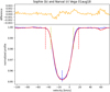 |
Fig. 1 Comparison of the LSD Stokes I intensity profile of Vega obtained with NARVAL/TBL and the new NEXTRA pipeline (red) and a quasi-simultaneous observation with SOPHIE/OHP (within one minute, blue), both processed with LSDpy. Stokes I profiles are quasi-identical. The difference of the SOPHIE and NARVAL profile is presented in the top panel (orange). Dashed blue line corresponds to the radial velocity of Vega of −13.9 km s−1. The dashed yellow lines show ±v sin i (21.6 km s−1), while the dashed red lines correspond to the outer limits of the profile including gaussian broadening (at additional ±10 km s−1). Data come from 1 August 2018 at 23:11 UT. |
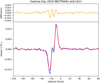 |
Fig. 2 Comparison of the LSD Stokes V profile of γ Equ generated with LSDpy and reduced with the new NEXTRA spectropolarimetric data reduction pipeline (blue) and reduced with the historic Libre-Esprit (red). Both pipelines provide quasi-identical results. The exact same dataset from 19 August 2018 is compared here. The difference between the NEXTRA and LE profile is given in the top panel (orange). |
3.2 Surface magnetic geometry
The successive time-series of Stokes V LSD profiles were used to reconstruct the surface magnetic field distribution of Vega at different epochs. For this, we employed the ZDI) inversion method (Semel 1989), using the Python code of Folsom et al. (2018a), based on the spherical harmonics formalism of Donati et al. (2006), the local line model of Folsom et al. (2018b), and assuming an oblate surface shape (Cang et al. 2020). The data preparation and ZDI input parameters we chose are identical to those adopted by Petit et al. (2022) for earlier observations of Vega (except that we adopted a rotation period of 0.678 d). The resulting reduced χ2 values are equal to 0.67, 0.55, and 0.28 in 2018, 2023, and 2024 (respectively). Three magnetic maps for observations taken in 2018, 2023, and 2024 are shown in Fig. 5.
The data gathered in 2018 were already presented by Petit et al. (2022), although the reduction code and LSD pipeline were different. Given the extremely weak signatures involved, it is interesting to note that the main magnetic features highlighted by Petit et al. (2022) survived this independent data reduction. The first one is the patch of radial negative field close to the pole and the second one is the equator-on dipole (the dominant reconstructed feature, storing 30–50% of the poloidal magnetic energy alone, depending on the epoch). Other small-scale magnetic patches display a lower consistency with our previous reconstruction, although some medium-sized magnetic spots do show up in both maps. The two newer maps, obtained from previously unpublished data of 2023 and 2024, confirm the long-term stability of the polar spot and inclined dipole. These characteristics are consistently recovered from data sets collected since 2008 (but do not show up if the Null profile is used instead of the Stokes V profile), enabling us to estimate a lifetime of 16 years, at least.
Here, we are dealing with observations where Zeeman signatures in individual LSD Stokes V profiles are dominated by noise, so that hundreds to thousands of LSD profiles must be combined in the tomographic inversion to extract a rotationally modulated signal. In such extreme situations, it is difficult to ensure that the tomographic inversion does not suffer from over-fitting. In other words, it is difficult to make sure that part of the recovered magnetic distribution does not originate from an attempt of the ZDI code to fit the noise pattern, especially at small spatial scales (as already stressed in Petit et al. 2022). This limitation is critical here, since rotationally modulated spectral features seen in Stokes I LSD profiles seem to be linked to surface regions smaller than the oblique dipole. The fact that small magnetic spots are not fully consistent in 2018, depending on the reduction code (i.e. between the map shown here and the one of Petit et al. 2022), is a further confirmation that small features should be considered with care (except for the polar spot, which benefits from an optimal visibility throughout the rotation cycle). Splitting the 2018 observations into two subsets to reconstruct two maps (either by taking every second observations or separating the first half from the second half of the observing epoch) led to similar conclusions. In spite of this warning, our magnetic maps suggest that some of the smaller magnetic regions do exhibit some consistency between epochs. The poles of the oblique dipole seem to co-exist with a higher geometrical complexity. This is the case, for instance, of the two spots of positive radial field seen in 2024 at phases 0.2 and 0.4 (inside the positive pole of the dipole), noting that similar features were visible in previous years as well.
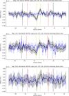 |
Fig. 3 Average Stokes V profile of Vega: 2018 (top), august 2023 (middle), and 2024 (bottom). Black line and grey zone: Averaged Stokes V and ±1 σ envelope. Blue line and 1 σ error bars: Averaged Null profile. Vertical dashed yellow lines show the position of the negative and positive peak of the 2018 averaged Stokes V profile. The dashed red lines show ±v sin i, while the dashed black lines correspond to the outer limits of the profile including gaussian broadening (additional ±10 km s−1) as shown in Fig. 1. |
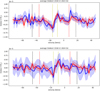 |
Fig. 4 Comparison of the average LSD Stokes V profile from NARVAL in 2018 (red) with profiles from NEO-NARVAL in august 2023 (top panel, blue) and 2024 (bottom panel, blue). Vertical lines are described in Fig. 3. |
4 Activity tracing results for starspots
Section 4.1 presents a redetermination of the rotation period based on rotational modulation of spectroscopic lines, while Sect. 4.2 offers an analysis of starspot signatures in the dynamic spectra of all datasets corresponding to the different observing seasons. Section 4.3 presents a newly developed reconstruction procedure for brightness maps and applies it to Vega. Finally, Sect. 4.4 summarises the search for correlation between magnetic field and activity structures.
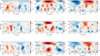 |
Fig. 5 ZDI reconstructions of magnetic geometries in equatorial projection for 2018, 2023, and 2024 (from top to bottom). Each column displays a component of the local magnetic vector, in a spherical coordinates frame. The field strength is colour-coded (in Gauss units). The phase reference was taken at BJD = 2456892.015, 2456892.185, and 2456892.506 for 2018, 2023, and 2024 (respectively) to ensure that all epochs display an oblique dipole pointing at the same phases. |
4.1 Rotation period redetermination
As mentioned earlier in this work, a first determination of the rotation period of Vega yielded ![Mathematical equation: $\[0.678_{-0.029}^{+0.036}\]$](/articles/aa/full_html/2025/10/aa56306-25/aa56306-25-eq2.png) d. It was detected in spectropolarimetric magnetic field observations (Alina et al. 2012) and confirmed by surface intensity observations (Böhm et al. 2015).
d. It was detected in spectropolarimetric magnetic field observations (Alina et al. 2012) and confirmed by surface intensity observations (Böhm et al. 2015).
In a next step, as described in Böhm et al. (2015), the bisector of the Stokes I LSD profiles was determined. The bisector velocity span (vspan) was calculated for each profile, measuring the difference between the upper and lower part of the bisector (a kind of skewness). For this purpose, we worked in relative profile height, the bottom of the profile set at 0., the continuum at 1. vspan was calculated as the difference of the medians of upper [0.35, 0.5] and lower [0.1, 0.25] bisector ranges.
Based on the assumption of a constant rotation period over the timescale of 6 years and based on the same measure (vspan), the new 2018 SOPHIE dataset enabled us to improve the precision of the period by combining with the results from SOPHIE 2012 dataset; a Lomb-Scargle (LS) analysis of the vspan yields a rotation period of 0.6771±0.0023 d, while a FELIX (Charpinet et al. 2010; Zong et al. 2016a; Zong et al. 2016b) vspan analysis based on multiperiodic non-linear least-squares fit produces an averaged rotation period of 0.6705 ± 0.0019 d (2012: 0.6679 ± 0.0016 d; 2018: 0.6730 ± 0.0001 d). Both determinations are within a 3-sigma interval from the original ![Mathematical equation: $\[0.678_{-0.029}^{+0.036}\]$](/articles/aa/full_html/2025/10/aa56306-25/aa56306-25-eq3.png) d period; however, an improvement of the error bar allowed us to assume a period of 0.6705 ± 0.0019 d, as produced by the FELIX time series analysis code. Figure 6 shows the frequency analysis of the vspan for the 2012 and 2018 dataset, superimposed are the redetermined rotation period. It should be noted that slight differences in rotation period determination may be a consequence of the fact that Vega is not likely in a solid body rotation; thus, different tracers might sense different areas of the star.
d period; however, an improvement of the error bar allowed us to assume a period of 0.6705 ± 0.0019 d, as produced by the FELIX time series analysis code. Figure 6 shows the frequency analysis of the vspan for the 2012 and 2018 dataset, superimposed are the redetermined rotation period. It should be noted that slight differences in rotation period determination may be a consequence of the fact that Vega is not likely in a solid body rotation; thus, different tracers might sense different areas of the star.
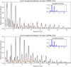 |
Fig. 6 LS periodogram of vspan (SOPHIE 2012: upper panel, 2018: lower panel), including the window function of the dataset. The rotational frequency of the star (1.492 d−1, for a period of 0.670 d), as well as its harmonics, are indicated by vertical bars with a height of 0.3. The lower bars at 0.15 and 0.02 height indicate the position of the ±1 and 2–day aliases, respectively, generated by the window function. |
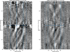 |
Fig. 7 Comparison of simultaneous 2018 Vega observations obtained with SOPHIE/OHP (left) and NARVAL/TBL (right). The two inner blue lines symmetric about zero velocity correspond to ±v sin i = 21.6 km s−1 (the profiles have been recentred to the rest velocity), while the outer dashed blue lines include the zone where gaussian broadening widens the line profile. Only 80% of the highest S/N files were kept for the dynamical spectra. White signatures designate bright spots on the star, grey scale varies from −0.0002 (white) to +0.0002 (black), values outside this scale are saturated in the figure. Phase zero corresponds to BJD = 2456892.015. |
4.2 Starspot signatures in dynamic spectra
After refining the rotational period of Vega we produced 2D dynamical spectra, as described in Böhm et al. (2015). To do so, we made use of the LSD I profiles described in Sect. 2. All individual observing times were rephased with a rotational period of P=0.678 d (for the sake of coherence with the magnetic maps) with respect to the same time reference used in the magnetic maps. For the 2012 data, phase zero corresponds to BJDref=2456142.332, for 2018, 2023 and 2024 BJDref = 2456892.015, 2456892.185, and 2456892.506, respectively). Therefore, for a given observing run, all magnetic and activity maps in this article can directly be compared. All LSD profiles were attributed to 128 phase bins and an individual median profile was calculated for each phase bin. To exhibit the very faint structures in the dynamic profile representation of Fig. 7, a mean profile was calculated throughout all spectra of a night and variations in line depth, radial velocity shifts of the profile, as well as offset variations (normalisation errors) were modeled via a linear model. The difference between the observations and an individual three parameter adjustment is then presented in the figure, as a function of velocity recentred on the stars rest frame (Vega having a radial velocity of −13.9 km s−1). At this stage, we do not know the origin of the starspots observed in Vega (Böhm et al. 2015). These might be differences in brightness, but this could also be related to local abundance variations or a combination of both. If it is brightness-related, a bright spot on the rotating star produces a local negative dip in the spectroscopic profile. According to the grey scale, a bright signature in the dynamical spectrum corresponds to a bright stellar spot. The typical brightness scale of dark and clear structures are ±1.5×10⁻⁴ F/Fc.
As a first step, we wanted to insure that two different datasets obtained simultaneously, namely, covering the same nights and reduced with different data reduction pipelines reproduce these very faint signatures in the same way. Figure 7 shows two dynamical Vega spectra from 2018 obtained with high precision velocimeter SOPHIE/OHP (left) and the spectropolarimeter NARVAL/TBL (right). Both figures cover the same observing period and have a starting period differing only by 1.6 minutes. SOPHIE data were reduced with the dedicated Sophie pipeline and NARVAL data with the new NEXTRA pipeline, while LSD profiles were produced in the identical way with LSDpy (see Sect. 2). We can see that the observations done with SOPHIE/OHP and NARVAL/TBL present exactly the same features, despite the fact that SOPHIE has a slightly higher spectral resolution. Therefore, we can confirm the reality of these very faint signatures.
The key focus of this section concerns the variability of surface brightness spots on Vega (assuming brightness and temperature is involved), while the surface magnetic field variations are analysed in Sect. 3. Dynamical spectra obtained with SOPHIE/OHP in 2012 (left) and 2018 (right) are compared in Fig. 9. Since the precision on the rotation period is too low to directly compare rephased dynamical spectra obtained with a time difference of roughly six years, a comparison must be made based on the shape of different features. To better understand these signatures it should be understood that a vertical signature close to the zero velocity line corresponds to an almost polar spot, while a sinusoidal signature crossing from the negative to positive velocity extreme (approx. ±30 km s−1) indicates a surface feature very close to the stellar equator. While the 2012 bright surface spots seem to cover all velocity domains, the 2018 bright spots seem to cover dominantly equatorial zones of the stellar surface. This can be seen for instance by comparing the average inclination of signatures crossing the profile or their velocity amplitudes. The signatures of the 2018 dynamic spectrum are systematically more inclined indicating a localisation nearer to the equator. Also, certain features present in the 2018 plot, for instance, the bright signature around phase 0.4 and maximum velocity are not seen at any phase in the 2012 dynamical spectra.
The contrast of the spectral signature (difference between brightest and darkest part of the signature) is very constant over the years 2012, 2018, 2023, and 2024, with a total maximal amplitude of 0.0003 with respect to the normalised continuum. The value of 0.0005 in the Böhm et al. (2015) has been refined in this paper to 0.0003 thanks to improved data reduction and rejection of poor-quality profiles.
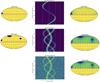 |
Fig. 8 Simulation of a spotted stellar surface in Mollweide projection and seen almost pole on as Vega. Deep blue are dark spots which appear in emission in the dynamical spectrum. Phase 0 is at the left of the stellar map (rotation vector points towards the top). Stellar rotation is counterclockwise in this representation. A spot at the central meridian of the stellar sphere (in front of the observer) would have phase zero and appear on the left of the map. Phases increase clockwise on the stellar sphere. If we read the map in analogy to the terrestrial coordinates, then the phase would correspond to the negative longitude. Left: original map of the stellar surface. Middle: dynamical spectrum. Right: reconstructed stellar surface map. Top: single spot. Middle: complex pattern of three spots of different sizes. Bottom: simulation of a realistic dynamical spectrum (signatures with an amplitude of 1.5 × 10⁻⁴ F/Fc and a noise of σ = 5 × 10⁵−5). |
4.3 Reconstruction of Vega’s brightness map
We used a pixel-based pattern matching approach to assess the spot density from the observed dynamical spectra. As can be seen in Fig. 8, each spot on a stellar surface shows a characteristic signature in the dynamical spectrum. Our basic reconstruction relays on this fact. To do so, we used a regular 128 × 128, colatitude × longitude grid over the (simplified spherical) star. Each cell of this grid defines a trace in the radial velocity × rotation phase plane, namely, the dynamical spectrum. We then summed the amplitude of the observed intensity along the trace specific to each grid-point we want to reconstruct. This provides us with a measure for the signed spot-intensity at this at this particular location of the stellar surface. This simple reconstruction of the spot distribution includes an amplitude bias related in first order to its colatitude. We therefore divided the reconstruction by this colatitude dependency to reduce this bias. However, the ‘spread’ bias due to the crossing of different signatures in the dynamical spectrum is not reduced that way. An application of the method is shown in the simulation of Fig. 8, including a realistic simulation with signature amplitudes and gaussian noise corresponding to our observations. Phase 0 is at the left of the stellar map (the rotation vector points towards the top), while phase 1 on the right. The stellar rotation is counterclockwise in this representation. A spot at the central meridian of the stellar sphere (in front of the observer) would be at phase zero and appear on the left of the map. Phases increase clockwise on the stellar sphere. In our figures, we adopted exactly the same colour scale for upper and lower boundaries.
Before reconstructing the observed stellar maps, we decided to exclude the most noisy parts of the 2018 dataset from the analysis: between phases 0.265–0.328 and 0.742–0.828 of Fig. 9 (top-right). All the reconstructed maps show the identical amplitude scale. Figures 9 and 10 (bottom panels) show the Mollweide projected reconstruction of 2012, 2018, 2023, and 2024 brightness maps. Bright stellar spots are represented in yellow on the reconstructed map. While in the 2012 data, diffuse bright spots at different latitude seem to coexist, the 2018 map concentrates its bright zones above the equator, higher latitudes seem to be less covered by bright zones. This indicates a variation in the surface spot distribution over 6 years. The 2023 and 2024 maps seem to confirm the dominant location of activity spots nearby Vega’s equator, despite the fact that the datasets were of lower quality. Still, the 2023 and 2024 maps are very different: the 2023 map shows two bright spots near the equator at phases 0.25 and 0.58, while the 2024 data shows a brighter spot at an approximately 30 degree latitude and close to phase 0. This tends to indicate spot variations within one year.
To verify the reality of the reconstructed spots versus pure noise we created an artificial dynamic spectrum with a random noise distribution (σ = 5 × 10⁻⁵), similar to the pure noise outside the spectral profile in the 2018 dataset, the signatures in the dynamic spectra having overall amplitudes of 3 ×10⁻⁴ F/Fc. Fig. 11 clearly shows that the reconstructed map only reveals fine fluctuations. A measurement shows that the bright and dark signatures well above the 3 σ noise level translate in the map representation in amplitude ranges at least twice above those corresponding to pure noise.
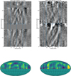 |
Fig. 9 Vega observations with SOPHIE/OHP in 2012 and 2018. Upper panels: dynamical spectra of 2012 and 2018. Phase zero corresponds for the 2018 dataset to BJD = 2456892.015. For the 2012 dataset, we opted for BJD = 2456142.332. The two inner blue lines symmetric to zero velocity correspond to ± v sin i = 21.6 km s−1, while the outer dashed blue lines include the zone where Gaussian broadening widens the line profile. Lower panels: reconstructed surface map of Vega in Mollweide projection, based on the procedure described in Sect. 4.2. Left: map of 2012. Right: map of 2018. Overall, 80% of the highest S/N files were kept for map building. |
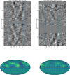 |
Fig. 10 Vega observations in 2023 (left) and 2024 (right) with NEO-NARVAL. See Fig. 9 caption for details. |
4.4 Search for a correlation between magnetic field and brightness maps
A major motivation behind the simultaneous observations with SOPHIE/OHP and NARVAL/TBL in 2018 was the analysis of magnetic versus activity spot location on the reconstructed stellar surface. First, we used a simple visual inspection to search for similarities between the reconstructed starspot map Fig. 9 (lower panel) and the surface magnetic field map Fig. 5 from 2018. Despite perfect alignment of the phase definition in the two representations, no obvious correspondence could be extracted (e.g. major activity spots located in equatorial regions with particularly strong radial or total magnetic field).
Since the dominant activity and magnetic features concentrate in regions near the equator, we decided to do a very rough one dimensional comparison of the location of magnetic versus activity spots in the enlarged equatorial belt of Vega, considering only latitudes between −7° and 45°, with the lower edge of this range being the most extremes areas of the map reconstruction visible on the nearby pole-on star. To do so, we summed quantities in longitude (or phase) strips: (i) the radial magnetic field strength; (ii) the total magnetic field strength (square root of the quadradic addition of radial, meridional and azimuthal field strength); and (iii) the starsport activity signature (intensity). This corresponds to project all information of the 2D maps on individual curves as a function of phase dependency only and omitting the latitude information. Three curves of the averaged radial magnetic field strength, total magnetic field strength, and activity signature as a function of phase were obtained (with a comparison in Fig. 12). At this stage, no obvious correlation between these curves could be drawn; therefore, there cannot report any indication of a correlation between the magnetic and activity spots.
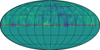 |
Fig. 11 Reconstructed surface map of a random noise dynamical spectrum. The standard deviation of the noise corresponds to the one measured outside the profile in the 2018 Sophie dynamical spectra. |
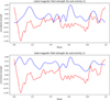 |
Fig. 12 Comparison of averaged latitudinal magnetic field strength variations (blue) and activity (red). Top: radial magnetic field and activity, bottom: total magnetic field strength and activity. |
5 Discussion and conclusions
The aim of our work is to better understand the origin and evolution of Vega’s faint observed stellar magnetic field. To this end, we are regularly monitoring Vega using high-resolution, high-cadence spectroscopy and spectropolarimetry to obtain a complete sampling of several times Vega’s short rotation period of ≈0.678 d over one observing run.
In this work, we managed to successfully cope with a major challenge, namely, to connect new datasets (e.g. 2023, 2024) obtained with a very different instrument (NEO-NARVAL) and a new data reduction pipeline (NEXTRA) to data obtained with NARVAL and reduced with the historic pipeline (LE), this despite the fact that magnetic signals are extremely faint in the case of Vega. We also demonstrated the robustness of our faint activity signatures by showing that they are identical in simultaneous datasets obtained with SOPHIE/OHP and NARVAL/TBL in 2018.
The spectropolarimetric observations of 2018, 2023, and 2024 obtained on Vega with NEO-NARVAL confirm the stability of the main magnetic signatures: a narrow polar spot of same average intensity during at least a decade and an inclined dipole indicating a localisation near to the equator and of comparable strength to previous observations. A stable magnetic field tends to support a fossil origin. However, small scale variations of the stellar magnetic field cannot be excluded, due to S/N and resolution limitations.
While Böhm et al. (2015) reports the first detection of starspots on a hot star like Vega, Petit et al. (2017) re-analysed the same SOPHIE dataset from 2012 and obtained hints of surface features evolving over the different nights of the observing run. In the current work, we were able to reveal long-term variations of the surface structure. A close comparison of our Mollweide projected maps of 2012 with those published in polar presentation by Petit et al. (2017) reveal strong similarities. Examining this line profile variability in three different ways leads to some consistent conclusions: (i) the analysis of Fig. 6 shows the presence of a significantly larger number of harmonics in the Lomb–Scargle periodogram of vspan. As shown in Fig. 6 in Böhm et al. (2015), this indicates a lower latitude of the spot location; (ii) a direct comparison of the dynamic spectra of 2012 and 2018 (shown in Fig. 9, upper panels) clearly shows that later dataset has significantly stronger gradients of the spot signatures crossing the spectra, moving towards more extreme velocities; (iii) the reconstructed stellar surface maps (presented in Fig. 9, lower panels) shows higher latitude bright emission spots in the 2012 dataset than in 2018. It is obvious that starspots are concentrated in equatorial regions of Vega. It is also interesting to notice that the normalised amplitude of the signatures in all the dynamic spectra (from 2012 to 2024) are very similar.
Despite the very weak magnetic field signatures in Vega, the magnetic maps suggest that the large-scale surface magnetic field remains stable over more than a decade (even up to 16 years). In contrast, the very weak intensity line profile variability most likely reveals surface spots that change on different time scales, with the 6 years between the two SOPHIE datasets serving as the upper limit. Based on the assumption that starspots are linked to magnetism, we consider the idea that variable starspots could be related to dynamo generated fields. We searched for similarities in spot distribution between the reconstructed starspot map of 2018 the surface magnetic field map, based on simultaneously obtained spectroscopic data at SOPHIE/OHP and spectropolarimetric data at NARVAL/TBL. While a final conclusion cannot be drawn from this limited dataset, it currently appears that the brightness spots are uncorrelated with the large-scale magnetic field.
The distribution and stability of the large scale magnetic field appear to be inconsistent with the distribution and variability of the brightness spots. If the variability in the line intensity profiles is indeed due to brightness spots, coupled with the possibility that these brightness spots are generated by magnetic fields (as seen in cooler stars), then this discrepancy could reflect two different components of the stellar magnetic field. The first would be a stable, large-scale component, contributing to the Stokes V signal. The second one is a variable, smaller scale component that would be strong enough to produce brightness spots, but structured in a sufficiently complex pattern of mixed magnetic polarities to mostly cancel out in Stokes V (noting that a similar possibility was pointed out by Blazère et al. 2020 for the Am star Alhena). We can speculate that the two components of the magnetic field have different origins. We also highlight the coexistence of a weak fossil field embedded in the radiative portion of the star (providing the stable, large-scale structure); whereas a convective dynamo, most likely concentrated in the equatorial regions where the convective envelope is deeper, could produce the variable, smaller scale structure.
Vega’s so-called magnetic puzzle is getting more mysterious thanks to new insights revealing simultaneous brightness and magnetic surface reconstructions. Thus, it is poised to deliver unique indications, enabling us to obtain deeper insights into the magnetism of tepid and hot stars.
Acknowledgements
The authors want to thank Alexis Lavail for fruitful discussions and support. CPF gratefully acknowledges funding from the European Union’s Horizon Europe research and innovation programme under grant agreement No. 101079231 (EXOHOST), and from the United Kingdom Research and Innovation (UKRI) Horizon Europe Guarantee Scheme (grant number 10051045). The specpolFLow can be found at https://github.com/folsomcp/specpolFlow and the LSDpy package at https://github.com/folsomcp/LSDpy. Matthias Hoschneider acknowledges financing the support of the DFG CRC research grant 1248 at Potsdam university.
References
- Alina, D., Petit, P., Lignières, F., et al. 2012, in American Institute of Physics Conference Series, 1429, eds. J. L. Hoffman, J. Bjorkman, & B. Whitney, 82 [Google Scholar]
- Aurière, M. 2003, in EAS Publications Series, 9, eds. J. Arnaud, & N. Meunier, 105 [Google Scholar]
- Balona, L. A. 2017, MNRAS, 467, 1830 [NASA ADS] [CrossRef] [Google Scholar]
- Balona, L. A. 2019, MNRAS, 490, 2112 [NASA ADS] [CrossRef] [Google Scholar]
- Blazère, A., Petit, P., Lignières, F., et al. 2016, A&A, 586, A97 [NASA ADS] [CrossRef] [EDP Sciences] [Google Scholar]
- Blazère, A., Petit, P., Neiner, C., et al. 2020, MNRAS, 492, 5794 [CrossRef] [Google Scholar]
- Böhm, T., Holschneider, M., Lignières, F., et al. 2015, A&A, 577, A64 [NASA ADS] [CrossRef] [EDP Sciences] [Google Scholar]
- Böhm, T., Cabanac, R., & Lopez Ariste, A. 2016, Technical Specifications, Tech. rep., Obs. Midi-Pyrénées [Google Scholar]
- Bouchy, F., Hébrard, G., Udry, S., et al. 2009, A&A, 505, 853 [NASA ADS] [CrossRef] [EDP Sciences] [Google Scholar]
- Bouchy, F., Díaz, R. F., Hébrard, G., et al. 2013, A&A, 549, A49 [NASA ADS] [CrossRef] [EDP Sciences] [Google Scholar]
- Braithwaite, J., & Cantiello, M. 2013, MNRAS, 428, 2789 [NASA ADS] [CrossRef] [Google Scholar]
- Cang, T. Q., Petit, P., Donati, J. F., et al. 2020, A&A, 643, A39 [NASA ADS] [CrossRef] [EDP Sciences] [Google Scholar]
- Cantiello, M., & Braithwaite, J. 2019, ApJ, 883, 106 [Google Scholar]
- Charpinet, S., Green, E. M., Baglin, A., et al. 2010, A&A, 516, L6 [NASA ADS] [CrossRef] [EDP Sciences] [Google Scholar]
- Donati, J.-F., Semel, M., Carter, B. D., Rees, D. E., & Collier Cameron, A. 1997, MNRAS, 291, 658 [NASA ADS] [CrossRef] [Google Scholar]
- Donati, J. F., Howarth, I. D., Jardine, M. M., et al. 2006, MNRAS, 370, 629 [NASA ADS] [CrossRef] [Google Scholar]
- Erba, C. 2024, in American Astronomical Society Meeting Abstracts, 243, 225.03 [Google Scholar]
- Folsom, C. P., Bouvier, J., Petit, P., et al. 2018a, MNRAS, 474, 4956 [NASA ADS] [CrossRef] [Google Scholar]
- Folsom, C. P., Fossati, L., Wood, B. E., et al. 2018b, MNRAS, 481, 5286 [Google Scholar]
- Folsom, C. P., Erba, C., Petit, V., et al. 2025, arXiv e-prints, [arXiv:2505.18476] [Google Scholar]
- Kanodia, S., & Wright, J. 2018, RNAAS, 2, 4 [NASA ADS] [Google Scholar]
- Kochukhov, O., Makaganiuk, V., & Piskunov, N. 2010, A&A, 524, A5 [NASA ADS] [CrossRef] [EDP Sciences] [Google Scholar]
- Lignières, F., Petit, P., Böhm, T., & Aurière, M. 2009, A&A, 500, L41 [CrossRef] [EDP Sciences] [Google Scholar]
- Meduri, D. G., Jouve, L., & Lignières, F. 2024, A&A, 683, A12 [NASA ADS] [CrossRef] [EDP Sciences] [Google Scholar]
- Perruchot, S., Kohler, D., Bouchy, F., et al. 2008, SPIE Conf. Ser., 7014, 70140J [Google Scholar]
- Petit, P., Lignières, F., Aurière, M., et al. 2011, A&A, 532, L13 [NASA ADS] [CrossRef] [EDP Sciences] [Google Scholar]
- Petit, P., Hébrard, E. M., Böhm, T., Folsom, C. P., & Lignières, F. 2017, MNRAS, 472, L30 [NASA ADS] [CrossRef] [Google Scholar]
- Petit, P., Böhm, T., Folsom, C. P., Lignières, F., & Cang, T. 2022, A&A, 666, A20 [NASA ADS] [CrossRef] [EDP Sciences] [Google Scholar]
- Petitdemange, L., Marcotte, F., Gissinger, C., & Daniel, F. 2024, A&A, 681, A75 [NASA ADS] [CrossRef] [EDP Sciences] [Google Scholar]
- Piskunov, N., Wehrhahn, A., & Marquart, T. 2021, A&A, 646, A32 [NASA ADS] [CrossRef] [EDP Sciences] [Google Scholar]
- Semel, M. 1989, A&A, 225, 456 [NASA ADS] [Google Scholar]
- Spruit, H. C. 2002, A&A, 381, 923 [CrossRef] [EDP Sciences] [Google Scholar]
- Takeda, Y. 2021, MNRAS, 505, 1905 [NASA ADS] [CrossRef] [Google Scholar]
- Takeda, Y., Kawanomoto, S., & Ohishi, N. 2008, ApJ, 678, 446 [NASA ADS] [CrossRef] [Google Scholar]
- Zechmeister, M., Anglada-Escudé, G., & Reiners, A. 2014, A&A, 561, A59 [NASA ADS] [CrossRef] [EDP Sciences] [Google Scholar]
- Zong, W., Charpinet, S., & Vauclair, G. 2016a, A&A, 594, A46 [NASA ADS] [CrossRef] [EDP Sciences] [Google Scholar]
- Zong, W., Charpinet, S., Vauclair, G., Giammichele, N., & Van Grootel, V. 2016b, A&A, 585, A22 [NASA ADS] [CrossRef] [EDP Sciences] [Google Scholar]
All Tables
All Figures
|
Fig. 1 Comparison of the LSD Stokes I intensity profile of Vega obtained with NARVAL/TBL and the new NEXTRA pipeline (red) and a quasi-simultaneous observation with SOPHIE/OHP (within one minute, blue), both processed with LSDpy. Stokes I profiles are quasi-identical. The difference of the SOPHIE and NARVAL profile is presented in the top panel (orange). Dashed blue line corresponds to the radial velocity of Vega of −13.9 km s−1. The dashed yellow lines show ±v sin i (21.6 km s−1), while the dashed red lines correspond to the outer limits of the profile including gaussian broadening (at additional ±10 km s−1). Data come from 1 August 2018 at 23:11 UT. |
| In the text | |
|
Fig. 2 Comparison of the LSD Stokes V profile of γ Equ generated with LSDpy and reduced with the new NEXTRA spectropolarimetric data reduction pipeline (blue) and reduced with the historic Libre-Esprit (red). Both pipelines provide quasi-identical results. The exact same dataset from 19 August 2018 is compared here. The difference between the NEXTRA and LE profile is given in the top panel (orange). |
| In the text | |
|
Fig. 3 Average Stokes V profile of Vega: 2018 (top), august 2023 (middle), and 2024 (bottom). Black line and grey zone: Averaged Stokes V and ±1 σ envelope. Blue line and 1 σ error bars: Averaged Null profile. Vertical dashed yellow lines show the position of the negative and positive peak of the 2018 averaged Stokes V profile. The dashed red lines show ±v sin i, while the dashed black lines correspond to the outer limits of the profile including gaussian broadening (additional ±10 km s−1) as shown in Fig. 1. |
| In the text | |
|
Fig. 4 Comparison of the average LSD Stokes V profile from NARVAL in 2018 (red) with profiles from NEO-NARVAL in august 2023 (top panel, blue) and 2024 (bottom panel, blue). Vertical lines are described in Fig. 3. |
| In the text | |
|
Fig. 5 ZDI reconstructions of magnetic geometries in equatorial projection for 2018, 2023, and 2024 (from top to bottom). Each column displays a component of the local magnetic vector, in a spherical coordinates frame. The field strength is colour-coded (in Gauss units). The phase reference was taken at BJD = 2456892.015, 2456892.185, and 2456892.506 for 2018, 2023, and 2024 (respectively) to ensure that all epochs display an oblique dipole pointing at the same phases. |
| In the text | |
|
Fig. 6 LS periodogram of vspan (SOPHIE 2012: upper panel, 2018: lower panel), including the window function of the dataset. The rotational frequency of the star (1.492 d−1, for a period of 0.670 d), as well as its harmonics, are indicated by vertical bars with a height of 0.3. The lower bars at 0.15 and 0.02 height indicate the position of the ±1 and 2–day aliases, respectively, generated by the window function. |
| In the text | |
|
Fig. 7 Comparison of simultaneous 2018 Vega observations obtained with SOPHIE/OHP (left) and NARVAL/TBL (right). The two inner blue lines symmetric about zero velocity correspond to ±v sin i = 21.6 km s−1 (the profiles have been recentred to the rest velocity), while the outer dashed blue lines include the zone where gaussian broadening widens the line profile. Only 80% of the highest S/N files were kept for the dynamical spectra. White signatures designate bright spots on the star, grey scale varies from −0.0002 (white) to +0.0002 (black), values outside this scale are saturated in the figure. Phase zero corresponds to BJD = 2456892.015. |
| In the text | |
|
Fig. 8 Simulation of a spotted stellar surface in Mollweide projection and seen almost pole on as Vega. Deep blue are dark spots which appear in emission in the dynamical spectrum. Phase 0 is at the left of the stellar map (rotation vector points towards the top). Stellar rotation is counterclockwise in this representation. A spot at the central meridian of the stellar sphere (in front of the observer) would have phase zero and appear on the left of the map. Phases increase clockwise on the stellar sphere. If we read the map in analogy to the terrestrial coordinates, then the phase would correspond to the negative longitude. Left: original map of the stellar surface. Middle: dynamical spectrum. Right: reconstructed stellar surface map. Top: single spot. Middle: complex pattern of three spots of different sizes. Bottom: simulation of a realistic dynamical spectrum (signatures with an amplitude of 1.5 × 10⁻⁴ F/Fc and a noise of σ = 5 × 10⁵−5). |
| In the text | |
|
Fig. 9 Vega observations with SOPHIE/OHP in 2012 and 2018. Upper panels: dynamical spectra of 2012 and 2018. Phase zero corresponds for the 2018 dataset to BJD = 2456892.015. For the 2012 dataset, we opted for BJD = 2456142.332. The two inner blue lines symmetric to zero velocity correspond to ± v sin i = 21.6 km s−1, while the outer dashed blue lines include the zone where Gaussian broadening widens the line profile. Lower panels: reconstructed surface map of Vega in Mollweide projection, based on the procedure described in Sect. 4.2. Left: map of 2012. Right: map of 2018. Overall, 80% of the highest S/N files were kept for map building. |
| In the text | |
|
Fig. 10 Vega observations in 2023 (left) and 2024 (right) with NEO-NARVAL. See Fig. 9 caption for details. |
| In the text | |
|
Fig. 11 Reconstructed surface map of a random noise dynamical spectrum. The standard deviation of the noise corresponds to the one measured outside the profile in the 2018 Sophie dynamical spectra. |
| In the text | |
|
Fig. 12 Comparison of averaged latitudinal magnetic field strength variations (blue) and activity (red). Top: radial magnetic field and activity, bottom: total magnetic field strength and activity. |
| In the text | |
Current usage metrics show cumulative count of Article Views (full-text article views including HTML views, PDF and ePub downloads, according to the available data) and Abstracts Views on Vision4Press platform.
Data correspond to usage on the plateform after 2015. The current usage metrics is available 48-96 hours after online publication and is updated daily on week days.
Initial download of the metrics may take a while.