© The Authors 2025

1. Introduction

Key aspects of helioseismology rely on a good understanding of the helioseismic observables. The relationship between intensity fluctuations and low-degree p modes has been extensively studied (see for example Toutain & Gouttebroze 1993, and references therein). In Kostogryz et al. (2021) (hereafter K+21), we extended this analysis to high-degree modes, incorporating radiative transfer effects and accounting for horizontal wave motions. Building on K+21, we advance this line of research in several significant ways. Firstly, we employ a more realistic background atmospheric model computed using the Merged Parallelized Simplified ATLAS code (MPS-ATLAS, Witzke et al. 2021). This model atmosphere accurately reproduces the observed limb darkening and consequently accounts for the spectral line formation height (Kostogryz et al. 2022). Secondly, we model the full spectral line rather than just the continuum intensity and compute Helioseismic and Magnetic Imager (HMI) observables from the model filtergrams using the algorithm described by Couvidat et al. (2012a) and referred to as the HMI LoS pipeline. Such an approach has recently been used by Petrie et al. (2025) to convert an MHD simulation into HMI magnetograms.

The observables are susceptible to various systematic errors due to instrumental limitations and potential misinterpretation caused by incomplete physical modeling. Here, we focus on two observables: the line-of-sight velocity (hmi.V_45s) and the continuum intensity (hmi.Ic_45s). It is worth noting that HMI does not observe continuum directly, and thus the continuum intensity computed by the HMI algorithm differs from the theoretical continuum intensity as derived, for example, by K+21.

While some corrections are applied in the LoS pipeline (Couvidat et al. 2016), residual systematic effects persist and are addressed differently depending on the helioseismic method. For instance, Bogart et al. (2015) and Liang et al. (2018) have investigated systematic errors in ring-diagram analysis and time-distance helioseismology, respectively. In this work, we aim to elucidate the impact of radiative transfer on the observed oscillations. Furthermore, we incorporate the effects of solar differential rotation and spacecraft velocity, the latter being identified as the most significant remaining systematic error in the observations (Couvidat et al. 2016).

The remainder of this paper is organized as follows. In Sect. 2, we present the spectral line obtained after applying radiative transfer in our background atmosphere. We then summarize the main steps of the HMI algorithm to compute observables from the intensity along the spectral line in Sect. 3. In Sect. 4, we analytically derive the first-order expressions for the observables when the background model is perturbed by oscillations. These expressions are then evaluated numerically to obtain HMI observables: line-of-sight velocity (hmi.V_45s) in Sect. 5 and continuum intensity (hmi.Ic_45s) in Sect. 6. Finally, we present our conclusions and outline some possible extensions of this work in Sect. 7.

2. Spectral synthesis in the background model

The Fe I 6173 Å line is observed by the HMI and Polarimetric and Helioseismic Imager (PHI; Solanki et al. 2020) space-based instruments and often used for photospheric diagnostics in ground-based observations (Cavallini 2006; Scharmer et al. 2007). This line was also chosen for the Photospheric Magnetic field Imager (PMI; Staub et al. 2020) that is to be flown on board ESA’s upcoming Vigil space mission. It is a diagnostically important photospheric spectral line that is used because of its large magnetic sensitivity (Landé factor of 2.5) and lack of (strong) blends that enables robust velocity inference.

We calculated the emergent intensity I_λ at wavelength λ (around the line central wavelength) for each point on the visible hemisphere using the following form of the formal solution of the radiative transfer equation:

$$\begin{array}{c}\hfill I_{\lambda }(\mu )={\displaystyle {\int }_0^{\infty }}{S}_{\lambda }({\tau }_{\lambda }){\text{e}}^{-{\tau }_{\lambda }/\mu }\frac{\mathrm{d}{\tau }_{\lambda }}{\mu },\end{array}$$(1)

where μ is the cosine of the angle between the line-of-sight vector and the local normal to the surface, with μ = 1 corresponding to disk center and μ = 0 to the limb. The source function S_λ was chosen as a Planck function by assuming local thermodynamic equilibrium. The optical depth, τ_λ, is obtained from the opacity, α_λ,

$$\begin{array}{c}\hfill {\tau }_{\lambda }(s;\mu )=-{\displaystyle {\int }_s^{\infty }}{\alpha }_{\lambda }(s^{\prime };\mu )\mathrm{d}{s}^{\prime },\end{array}$$(2)

where s is the geometric height. Numerically, the integration in Eq. (1) needs to be performed only on the optically thin layers (we used layers where the optical depth in the continuum is between 10⁻⁸ and 60).

2.1. Background model

A background model (temperature, pressure, density) that accurately reflects the conditions in the solar atmosphere is crucial for realistic modeling of the spectral line. We used a plane-parallel atmosphere, which is a reasonable approximation to compute radiative transfer for the Sun (except very close to the limb), as the atmosphere is thin compared to the solar radius (see, for example, Toutain et al. 1999, for a comparison of intensity in plane-parallel and spherical geometries).

We opted for a solar atmosphere model from a grid of stellar models by Kostogryz et al. (2022) computed with the MPS-ATLAS code adopting chemical abundances from Asplund et al. (2009). This model includes convection in the lower atmospheric layers, using the mixing-length approximation, and accounts for overshoot from the convective zone into the atmosphere, extending up to one pressure scale height. This background model has been extensively tested against solar measurements (Witzke et al. 2021; Kostogryz et al. 2022) and has shown very good agreement with solar limb darkening observations. This implies that the model allows for an accurate treatment of the formation height dependence on disk position and justifies its choice for the present study.

To model oscillations up to the photosphere (where the observed signal is formed), we used a global eigenvalue solver that requires a model for the solar interior. We used the standard solar Model S (Christensen-Dalsgaard et al. 1996) from the solar center to 700 km below the surface. We smoothly patched it to the atmospheric model from Kostogryz et al. (2022). A smooth transition between these two models was implemented close to the surface as shown in Fig. 1 for density and sound speed. We note that any type of perturbation can be used in the setup presented here. We could have also used outputs from numerical simulations or eigenfunctions computed in a Cartesian box using the plane-parallel approximation.

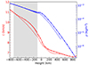Fig. 1. Background sound speed (red) and density (blue) from Model S (dashed), MPS-ATLAS (solid), and the patched model used in this study (dots). The gray region represents the domain where the patching between Model S and MPS-ATLAS is done. The zero level of height in this context is defined at one solar radius.

2.2. Opacity of the Fe I 6173 Å line and continuum

We computed the opacity, α_λ, as the sum of the Fe I line opacity and the continuum opacity employing the high-resolution mode of the MPS-ATLAS code. For the line opacity computation, we selected the Fe I line at λ = 6175.04 Å from the list of atomic lines provided by the Vienna Atomic Line Database (VALD; Piskunov et al. 1995; Kupka et al. 1999; Ryabchikova et al. 2015), which correspond to λ = 6173.33 Å after conversion from vacuum to air wavelength. The shape of the spectral line opacity was approximated by a Voigt profile. In addition, we accounted for the Doppler broadening using a depth-independent micro-turbulent velocity of 1 km/s.

To compute the continuum opacities, we included free-free and bound-free transitions in H⁻, H, He, He⁻, C, N, O, Ne, Mg, Al, Si, Ca, Fe; the molecules CH, OH, and NH; and their ions for the absorption continuum opacity calculation. For the scattering contribution, we considered electron scattering and Rayleigh scattering on HI, HeI, and H₂.

2.3. Spectral line broadening

We synthesized the Fe I spectral line in a 1D geometry by solving Eq. (1) with constant micro-turbulent velocity, resulting in a symmetric (unperturbed) spectral line profile. This approach neglects the upflow and downflow motions caused by granulation, which contribute to line broadening and introduce line asymmetries. Accurately modeling these effects would require synthesizing spectra using a three-dimensional hydrodynamic simulation or using a depth-dependent micro-turbulent velocity, which is beyond the scope of this paper. However, to account for line broadening due to granulation, we computed the emergent intensity by convolving the synthesized intensity profile with a broadening kernel (Gray 2021):

$$\begin{array}{c}\hfill \stackrel{\sim }{I}(\lambda ,\mu )=[I(\mu )\ast G_{\mathrm{macro}}(\mu )](\lambda ),\end{array}$$(3)

where * denotes a convolution with respect to wavelength and G_macro is a Gaussian kernel of standard deviation σ_macro. To account for the effect that granulation broadens spectral lines differently from the center to the limb, we adopted the standard deviation proposed by Takeda & UeNo (2019) that depends on the position on the disk:

$$\begin{array}{c}\hfill {\sigma }_{\mathrm{macro}}={\sigma }_0+{\sigma }_1\sqrt{1-{\mu }^2}.\end{array}$$(4)

To achieve the correct line broadening, we tuned the parameters σ₀ and σ₁ to match the spectral line observations at different μ-positions from Ellwarth et al. (2023) and obtained σ₀ = 0.95 km/s and σ₁ = 0.5 km/s.

2.4. Center-to-limb variation of background intensity

In Figure 2, we compare observed and modeled center-to-limb intensity variations in the continuum (left panel) and spectral line (right panel) using the MPS-ATLAS background model. We also compare with Model S, as it was used in our previous study to compute intensity (K+21) and is often used in helioseismology. Here, the background intensity refers to the emergent intensity computed in an unperturbed atmosphere, serving as the reference for subsequent analysis. The limb darkening observation was conducted by Neckel & Labs (1994) in quiet regions of the Sun. They fit a fifth-order polynomial in μ in the continuum at various wavelengths, and we selected the values at 6110 Å for comparison. Both models align well with the limb-darkening observational data for μ ≥ 0.2. For lower values of μ, the MPS-ATLAS background model reproduces the observations more accurately. The close alignment in center-to-limb variations in emergent intensity between the observations and models indicates that the background model reliably represents the atmospheric structure where the continuum forms.

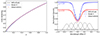Fig. 2. Background intensity computed from the MPS-ATLAS solar model atmosphere (solid), the standard solar Model S (dashed), and from the observations (dots). Left: Limb darkening (Ic(μ)/Ic(μ = 1)) in the continuum around the HMI line compared with the observations from Neckel & Labs (1994). Right: Synthesized FeI spectral line background intensity ($\stackrel{\sim }{I}(\lambda ,\mu )/I_c(\mu =1)$) compared with the observations from the IAG spectral atlas (Ellwarth et al. 2023) at μ = 1 (blue) and μ = 0.5 (red). The wavelength offset is with respect to the center of the HMI line λHMI = 6173.33 Å. The black dashed curves represent the six HMI filtergrams.

We also compared the spectral line profiles between our models and the observations from Ellwarth et al. (2023) at two positions on the disk. The intensity computed with the MPS-ATLAS model reproduces well the observed spectral line depth and width, while the spectral line depth obtained from Model S is too deep. It shows that the atmospheric layers where the line core forms are not realistic for Model S. Since our objective is to compute Doppler velocities, it is crucial to accurately reproduce the spectral line around the instrument’s central wavelength, and we therefore use the MPS-ATLAS background model in the remainder of the paper.

3. HMI algorithm for continuum intensity and velocity

The observed intensities were acquired at a small number of filtergrams, N (six for HMI), corresponding to the convolution of the wavelength-dependent intensities with filters, F_j, centered around specific wavelengths, λ_j:

$$\begin{array}{c}\hfill {\mathcal{I}}_j(\mu )={\displaystyle {\int }_{-\infty }^{\infty }}{F}_j(\lambda )\stackrel{\sim }{I}(\lambda ,\mu )\mathrm{d}\lambda .\end{array}$$(5)

In Figure 2, we show the spectral shapes of the HMI filters at the disk center. Here, two filters are primarily located in the continuum: two in the wings of the line and two closer to the line core. The filters vary across the field of view (Couvidat et al. 2012b), but this effect is not taken into account in this study. Since the filters are distributed near the central wavelength of the line, the integral in Eq. (5) can be evaluated over a narrow wavelength range. We considered only one spectral line and computed Eq. (5) as

$$\begin{array}{c}\hfill {\mathcal{I}}_j(\mu )={\displaystyle {\int }_{{\lambda }_{\mathrm{HMI}}-0.3}^{{\lambda }_{\mathrm{HMI}}+0.3}}{F}_j(\lambda )\stackrel{\sim }{I}(\lambda ,\mu )\mathrm{d}\lambda +I_c(\mu ){\displaystyle {\int }_{|\lambda -{\lambda }_{\mathrm{HMI}}|>0.3}}{F}_j(\lambda )\mathrm{d}\lambda ,\end{array}$$(6)

where λ_HMI is expressed in Å. The second integral takes into account that the filters are non-zero in a broader range of frequencies. We assumed that I_λ = I_c for |λ − λ_HMI|> 0.3 Å and neglected the (weak) blends from other lines for simplicity.

From the six intensities, the main quantities to compute continuum intensities and velocities using the HMI algorithm are the Fourier coefficients a₁ and b₁:

$$\begin{array}{cc}\hfill a_1(\mu )& =\frac{2}{N}{\displaystyle \sum _{j=1}^N}{\mathcal{I}}_j(\mu )cos\left(2\pi \frac{N-0.5-j}{N}\right),\hfill \end{array}$$(7)

$$\begin{array}{cc}\hfill b_1(\mu )& =\frac{2}{N}{\displaystyle \sum _{j=1}^N}{\mathcal{I}}_j(\mu )sin\left(2\pi \frac{N-0.5-j}{N}\right).\hfill \end{array}$$(8)

The second Fourier coefficients, a₂ and b₂, were computed in the same manner by replacing 2π by 4π in the cos and sin.

3.1. Velocity

The Doppler velocity was computed as (Couvidat et al. 2012a)

$$\begin{array}{c}\hfill \mathrm{v}(\mu )=V_{\mathrm{dop}}\text{atan2}[b_1(\mu ),a_1(\mu )],\end{array}$$(9)

where the coefficient V_dop  is usually written as

$$\begin{array}{c}\hfill V_{\mathrm{dop}}=\frac{\mathrm{d}v}{\mathrm{d}\lambda }\frac{T}{2\pi }.\end{array}$$(10)

The period of the observation wavelength span is T = 6 × 68.8 = 412.8 mÅ for HMI, which gives V_dop  ≈ 2.91 km/s. However, it needs to be calibrated via a look-up table due to the limited number of available wavelengths and the filters (Scherrer et al. 1995; Couvidat et al. 2012a). The HMI Doppler velocity (hmi.V_45s) is thus given as

$$\begin{array}{c}\hfill {\mathrm{v}}_{\mathrm{HMI}}={\mathcal{F}}_{\mathrm{HMI}}(\mathrm{v},\mu ),\end{array}$$(11)

where ℱ_HMI corresponds to the look-up table (see Appendix B for more details). For not too strong background velocities (less than 3 km/s), this function is almost the identity, and thus v_HMI ≈ v (see Fig. B.1). However, it deviates from the identity for large background velocities and/or small values of μ. We note that in the production code, due to an initial implementation error, T = 5 × 68.8 mÅ is used (Couvidat et al. 2012a). This effect is compensated by the look-up table as long as the slope between δv and δv_HMI is linear but can become significant for large background velocities (larger than 5 km/s, see Fig. B.1).

3.2. Continuum intensity

As for velocity, the continuum intensity (hmi.Ic_45s) was computed from the Fourier coefficients

$$\begin{array}{c}\hfill I_{\mathrm{HMI}}(\mu )=\frac{1}{6}{\displaystyle \sum _{j=1}^N}[{\mathcal{I}}_j(\mu )+I_d(\mu )\text{exp}(-\frac{{({\lambda }_j-{\lambda }_{\mathrm{HMI}})}^2}{{\sigma }^2(\mu )})],\end{array}$$(12)

where the estimate of the line width is

$$\begin{array}{c}\hfill \sigma (\mu )=\frac{T}{\pi \sqrt{6}}\sqrt{log\left(\frac{a_1^2(\mu )+b_1^2(\mu )}{a_2^2(\mu )+b_2^2(\mu )}\right)},\end{array}$$(13)

and that of the line depth is

$$\begin{array}{c}\hfill I_d(\mu )=\frac{T}{2\sqrt{\pi }\sigma (\mu )}\sqrt{a_1^2(\mu )+b_1^2(\mu )}exp\left(\frac{{\pi }^2{\sigma }^2(\mu )}{T^2}\right).\end{array}$$(14)

4. First-order perturbations for observables

Similar to the approach used by K+21 for the theoretical continuum intensity, we wanted to evaluate the perturbed intensity and velocity caused by the oscillations. We linearized around a background state that represents a spherically symmetric Sun characterized by its temperature, T₀; pressure, p₀; background velocity, u₀ (for example, rotation); and normal vector, r₀ = r₀e_r, at the unperturbed radial coordinate, r₀. The oscillations perturb the surface

$$\begin{array}{c}\hfill \mathit{r}={\mathit{r}}_0+\mathit{\xi },\end{array}$$(15)

where ξ is the Lagrangian displacement vector, which is linked to the Eulerian velocity through

$$\begin{array}{c}\hfill \mathit{u}={\partial }_t\mathit{\xi }-\mathit{\xi }·\mathrm{\nabla }{\mathit{u}}_0.\end{array}$$(16)

The oscillations also modify the thermodynamical quantities T = T₀ + δT, p = p₀ + δp, where the δ corresponds to Lagrangian perturbations. In this paper, we perturbed the surface by the oscillations of a single global mode (see Sect. 5), but the theoretical framework presented below is general. A summary of the different quantities in their background and perturbed state is given in Tab. 1.

This approach is in line with the idea of the response functions used in solar spectropolarimetric diagnostics (e.g., Beckers & Milkey 1975; Landi Degl’Innocenti & Landi Degl’Innocenti 1977; Milić & van Noort 2017). The idea behind the response functions is to devise a kernel that expresses the sensitivity of the emergent (generally, polarized) spectrum to the perturbations of specific physical quantities (temperature, pressure, velocity, magnetic field) in the atmosphere. This kernel is then used to design the observations or to fit the model atmosphere to the observed spectra, i.e., conduct spectropolarimetric inversion. Recently, an interesting application of the response functions, following concepts from helioseismology, has been proposed by Agrawal et al. (2023).

4.1. Perturbed intensity

In the continuum, the perturbed intensity can be written as a sum of purely thermodynamical terms (depending only on δT or δp) and geometrical terms (depending on all the components of the displacement ξ) (see, e.g., K+21). In the line, an additional term corresponding to a Doppler shift appears, and the perturbed intensity can be written as

$$\begin{array}{c}\hfill \delta I_{\lambda }(\mu )=\delta I_{\mathrm{th}}(\lambda ,\mu )+\delta I_{\mathrm{geom}}(\lambda ,\mu )+\delta I_{\mathrm{line}}(\lambda ,\mu ).\end{array}$$(17)

This last term is due to the dependency of opacity on the line-of-sight velocity

$$\begin{array}{c}\hfill {\mathrm{v}}_{\mathrm{los}}^0={\mathit{u}}_0·{\mathbf{e}}_{\mathrm{obs}},\end{array}$$(18)

where e_obs points toward the observer (see, e.g., Eq. (A.12) in K+21 for its expression in spherical coordinates). The variations of the opacity α(p, T, v_los) are obtained from

$$\begin{array}{c}\hfill \frac{\delta {\alpha }_{\lambda }}{{\alpha }_{\lambda }^0}=\frac{\partial (log{\alpha }_{\lambda }^0)}{\partial (log{p}_0)}\frac{\delta p}{p_0}+\frac{\partial (log{\alpha }_{\lambda }^0)}{\partial (log{T}_0)}\frac{\delta T}{T_0}+\frac{\partial (log{\alpha }_{\lambda }^0)}{\partial {\mathrm{v}}_{\mathrm{los}}^0}\delta {\mathrm{v}}_{\mathrm{los}},\end{array}$$(19)

where the derivative in the last term can be calculated as

$$\begin{array}{c}\hfill \frac{\partial (log{\alpha }_{\lambda }^0)}{\partial {\mathrm{v}}_{\mathrm{los}}^0}=\frac{\partial (log{\alpha }_{\lambda }^0)}{\partial \lambda }\frac{\partial \lambda }{\partial {\mathrm{v}}_{\mathrm{los}}^0}=\frac{\partial (log{\alpha }_{\lambda }^0)}{\partial \lambda }\frac{\lambda }{c}.\end{array}$$(20)

The thermodynamical and geometrical terms are derived in K+21, and we recall their formulation here for completeness. The geometrical term depends on the displacement and its derivatives and is given by

$$\begin{array}{cc}\hfill \delta I_{\mathrm{geom}}(\lambda ,\mu )=& \frac{1}{{\mu }_0}{\displaystyle {\int }_0^{\infty }}{r}_0{S}_{\lambda }^0{e}^{-{\tau }_{\lambda }^0/{\mu }_0}\{\frac{\partial }{\partial r_0}\left(\frac{\mathit{\xi }·{\mathit{e}}_{\text{obs}}}{r_0}\right)\hfill \\ \hfill & +(\frac{{\tau }_{\lambda }^0}{{\mu }_0}-1)({\mu }_0\frac{\partial }{\partial r_0}\left(\frac{{\xi }_r}{r_0}\right)-\frac{\mathrm{\nabla }\mathit{\xi }·{\mathit{e}}_{\mathrm{obs}}}{r_0})\}\frac{\mathrm{d}{\tau }_{\lambda }^0}{{\mu }_0}.\hfill \end{array}$$(21)

The thermodynamical term reflects the changes in the opacity and source function and can be written as

$$\begin{array}{c}\hfill \delta I_{\mathrm{th}}(\lambda ,\mu )={\displaystyle {\int }_0^{\infty }}[f_T^{\lambda }\frac{\delta T}{T_0}+f_P^{\lambda }\frac{\delta p}{p_0}]{\text{e}}^{-{\tau }_{\lambda }^0/{\mu }_0}\frac{\mathrm{d}{\tau }_{\lambda }^0}{{\mu }_0},\end{array}$$(22)

where the functions f_T and f_P are given by

$$\begin{array}{cc}\hfill f_T^{\lambda }({\tau }_{\lambda }^0,{\mu }_0)& =S_{\lambda }^0\frac{h\nu /k{T}_0}{1-{\text{e}}^{-h\nu /k{T}_0}}+\frac{\partial log{\alpha }_{\lambda }^0}{\partial log{T}_0}[S_{\lambda }^0-I_{\lambda }^0],\hfill \end{array}$$(23)

$$\begin{array}{cc}\hfill f_P^{\lambda }({\tau }_{\lambda }^0,{\mu }_0)& =\frac{\partial log{\alpha }_{\lambda }^0}{\partial log{p}_0}[S_{\lambda }^0-I_{\lambda }^0].\hfill \end{array}$$(24)

The relation from K+21 has been integrated by parts to make appear the background intensity, I_λ⁰, an expression already obtained by Zhugzhda et al. (1996) (see Appendix D). Using Eq. (21) from K+21 that relates the perturbed intensity to the change in opacity, we obtained the perturbations due to the line-of-sight velocity:

$$\begin{array}{c}\hfill \delta I_{\mathrm{line}}(\lambda ,\mu )={\displaystyle {\int }_0^{\infty }}\frac{\partial log{\alpha }_{\lambda }^0}{\partial \lambda }\frac{\lambda }{c}[S_{\lambda }^0-I_{\lambda }^0]\delta {\mathrm{v}}_{\mathrm{los}}{\text{e}}^{-{\tau }_{\lambda }^0/{\mu }_0}\frac{\mathrm{d}{\tau }_{\lambda }^0}{{\mu }_0}.\end{array}$$(25)

This term shifts the spectral line and is the main contributor to the velocity, as we demonstrate in the numerical section (Sect. 5).

4.2. Perturbed velocity

We show in App. C.1 that v = v⁰ + δv, where

$$\begin{array}{cc}\hfill {\mathrm{v}}^0& =V_{\mathrm{dop}}\text{atan2}[b_1^0,a_1^0],\hfill \end{array}$$(26)

$$\begin{array}{cc}\hfill \delta \mathrm{v}& =V_{\mathrm{dop}}\frac{{\displaystyle {\sum }_{i=1}^N{\sum }_{j=1}^N}{\mathcal{I}}_i^0\delta {\mathcal{I}}_{j}sin\left(2\pi \frac{j-i}{N}\right)}{{\displaystyle {\sum }_{i=1}^N{\sum }_{j=1}^N}{\mathcal{I}}_i^0{\mathcal{I}}_j^{0}cos\left(2\pi \frac{j-i}{N}\right)}.\hfill \end{array}$$(27)

The perturbed filtergrams, δℐ_j, such that ℐ_j = ℐ_j⁰ + δℐ_j were computed from Eq. (5) using the perturbed intensities derived in the previous section.

The look-up table needs to be taken into account to compute the perturbed HMI velocity. Using Eq. (11),

$$\begin{array}{c}\hfill {\mathrm{v}}_{\mathrm{HMI}}={\mathcal{F}}_{\mathrm{HMI}}({\mathrm{v}}^0+\delta \mathrm{v},{\mu }_0+\delta \mu )={\mathrm{v}}_{\mathrm{HMI}}^0+\delta {\mathrm{v}}_{\mathrm{HMI}},\end{array}$$(28)

where the expression for δμ is given by Eq. (18) in K+21 and

$$\begin{array}{cc}\hfill {\mathrm{v}}_{\mathrm{HMI}}^0& ={\mathcal{F}}_{\mathrm{HMI}}({\mathrm{v}}^0,{\mu }_0),\hfill \end{array}$$(29)

$$\begin{array}{cc}\hfill \delta {\mathrm{v}}_{\mathrm{HMI}}& =\delta \mathrm{v}\frac{\partial {\mathcal{F}}_{\mathrm{HMI}}}{\partial \mathrm{v}}+\delta \mu \frac{\partial {\mathcal{F}}_{\mathrm{HMI}}}{\partial \mu }.\hfill \end{array}$$(30)

A representation of the function ℱ_HMI and its derivatives is given in Appendix B.

4.3. Response function for velocity

To simplify the computation and the interpretation of the measured velocity, a direct relationship between δv and δv_los = u ⋅ e_obs would be helpful. This can be constructed for the term coming from δI_line, which we denote as δv_line. First, rewrote δI_line defined in Eq. (25) as

$$\begin{array}{c}\hfill \delta I_{\mathrm{line}}(\lambda ,\mu )={\displaystyle {\int }_0^{\infty }}{K}_I(\lambda ,s,{\mu }_0)\delta {\mathrm{v}}_{\mathrm{los}}(s,{\mu }_0)\mathrm{d}s,\end{array}$$(31)

where s is the geometrical height defined from Eq. (2) and

$$\begin{array}{c}\hfill K_I(\lambda ,s,{\mu }_0)=-\frac{\partial log{\alpha }_{\lambda }^0}{\partial \lambda }\frac{\lambda }{c}[S_{\lambda }^0-I_{\lambda }^0]\frac{{\alpha }_{\lambda }^0}{{\mu }_0}{\text{e}}^{-{\tau }_{\lambda }^0/{\mu }_0}.\end{array}$$(32)

Then, using Eq. (27), we obtained

$$\begin{array}{c}\hfill \delta {\mathrm{v}}_{\mathrm{line}}({\mu }_0)={\displaystyle {\int }_0^{\infty }}K(s;{\mu }_0)\delta {\mathrm{v}}_{\mathrm{los}}(s,{\mu }_0)\mathrm{d}s,\end{array}$$(33)

where

$$\begin{array}{c}\hfill K(s;{\mu }_0)=\frac{\partial {\mathcal{F}}_{\mathrm{HMI}}}{\partial {\mathrm{v}}^0}{V}_{\mathrm{dop}}\frac{{\displaystyle {\sum }_{i,j}}{\mathcal{I}}_i^0({\mu }_0){\mathcal{K}}_j(s;\mu )sin\left(2\pi \frac{j-i}{N}\right)}{{\displaystyle {\sum }_{i,j}}{\mathcal{I}}_i^0({\mu }_0){\mathcal{I}}_j^0({\mu }_0)cos\left(2\pi \frac{j-i}{N}\right)},\end{array}$$(34)

with

$$\begin{array}{c}\hfill {\mathcal{K}}_j(s;{\mu }_0)={\displaystyle {\int }_{-\infty }^{\infty }}{F}_j(\lambda ){[K_I(s,{\mu }_0)\ast G_{\mathrm{macro}}({\mu }_0)]}_{\lambda }\mathrm{d}\lambda .\end{array}$$(35)

A representation of this kernel, K, is given in Fig. 3, and it shows that the observed velocity corresponds to a weighted average of the oscillation velocity at different depths. This averaging depends on the center-to-limb distance, particularly for small values of μ (μ ≤ 0.2). Close to the disk center, the maximum is obtained around 120 km above the surface, and the center-of-gravity is at 180 km. These values are in agreement with the formation heights reported by Fleck et al. (2011) and Nagashima et al. (2014) using the HMI algorithm on 3D radiation-hydrodynamic simulations. However, this function is far from a delta function (with height), and the observed velocity corresponds to a weighted averaging from the surface to about 400 km above the surface at the disk center. A similar approach was undertaken by Vukadinović et al. (2022) to construct a kernel that relates the weak-field estimate of the line-of-sight magnetic field to the underlying depth-dependent field. Finally, we note that Eq. (35) can be used to define a response function and a formation height for the six measured HMI intensities.

Fig. 3. Response function for velocity K(s, μ) (in Mm−1) defined by Eq. (34) as a function of height, s, and limb angle, μ. The black and white lines respectively represent the maximum and center of gravity of the response function for each value of μ.

4.4. Perturbed continuum intensity

The perturbed continuum intensity was obtained in a similar way to velocity. In Appendix C.3, we derived

$$\begin{array}{c}\hfill \delta I_{\mathrm{HMI}}=\frac{1}{N}{\displaystyle \sum _{j=1}^N}\delta {\mathcal{I}}_j+{\mathrm{e}}^{-\frac{{({\lambda }_j-{\lambda }_{\mathrm{HMI}})}^2}{{\sigma }_0^2}}(\delta I_d+2I_d^0\frac{\delta \sigma }{{\sigma }_0}\frac{{({\lambda }_j-{\lambda }_{\mathrm{HMI}})}^2}{{\sigma }_0^2}),\end{array}$$(36)

where the perturbed line width and line depth are

$$\begin{array}{cc}\hfill \delta \sigma & =\frac{T^2}{6{\pi }^2{\sigma }_0}[\frac{a_1^0\delta a_1+b_1^0\delta b_1}{{(a_1^0)}^2+{(b_1^0)}^2}-\frac{a_2^0\delta a_2+b_2^0\delta b_2}{{(a_2^0)}^2+{(b_2^0)}^2}],\hfill \end{array}$$(37)

$$\begin{array}{cc}\hfill \delta I_d& =I_d^0[-\frac{\delta \sigma }{{\sigma }_0}+\frac{\delta a_1{a}_1^0+\delta b_1{b}_1^0}{{(a_1^0)}^2+{(b_1^0)}^2}+\frac{2{\pi }^2{\sigma }_0\delta \sigma }{T^2}].\hfill \end{array}$$(38)

We note that the line width and line depth are also HMI observables (hmi.Lw_45s and hmi.Ld_45s respectively), but we do not study them in detail here.

4.5. Validation

To assess whether the intensity perturbation using the first-order perturbation theory functions correctly, we first present a validation of our algorithm. We perturbed the background model from Sect. 2 characterized by (r₀, p₀, T₀) and intensity, I_λ⁰, using a simple function representative of a radial eigenfunction. We then computed the intensity, I^λ(μ), at each wavelength in the perturbed medium, which has a surface given by r₀e_r + ξ; velocity, d_tξ; pressure, p = p₀ + δp; and temperature, T = T₀ + δT. The difference between the perturbed and background intensity, I_λ − I_λ⁰, was then compared to the first-order computation of δI_λ derived in Sect. 4.1.

In Fig. 4, we compare the different contributions separately, for example, I_th is computed in a background medium with perturbed pressure and temperature but without surface deformation or velocity. The direct and first-order computations agree very well for the different contributions, which allowed us to validate the derivation in Sect. 4.1 and the numerical implementation.

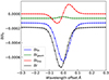Fig. 4. Test of the direct computation of the perturbed intensity (Iλ − Iλ0)/Iλ0 (dots) for μ = 0.5 and comparison with first-order computations δIλ/Iλ0 (solid line). The thermodynamic, geometrical, and line contributions are represented separately in blue, green, and red, while the full intensity is in black. The wavelength offset is with respect to the center of the HMI line λHMI = 6173.33 Å.

Once the intensity was known at all wavelengths, the continuum intensity and the velocity could be computed following the HMI algorithm. A comparison of these two observables, obtained from both the direct computation and the first-order formulation, is presented in Appendix A, Figs. A.2 and A.1, for the HMI velocity and continuum intensity. Both methods agree well, validating the expressions of δv (Eq. (27)) and δI_HMI (Eq. (36)).

5. HMI line-of-sight Doppler velocity

The interpretation of Doppler velocity often relies on the assumption that the observed Doppler velocity is simply a line-of-sight projection at a given height. In this section, we study how our more comprehensive approach differs from this simple approximation. We considered the different terms that enter into the computation of the HMI velocity:

$$\begin{array}{c}\hfill \delta {\mathrm{v}}_{\mathrm{HMI}}=\delta {\mathrm{v}}_{\mathrm{line}}+\delta {\mathrm{v}}_{\mathrm{th}}+\delta {\mathrm{v}}_{\mathrm{geom}}.\end{array}$$(39)

The framework developed here is general and could be used with any perturbation. Here, we perturbed our atmosphere by a single mode, ξ_nl, associated with the eigenfrequency, ω_nl, and computed the resulting velocity, δv_HMI. The eigenfunctions were computed in a (non-rotating) spherically symmetric background and thus do not depend on the longitudinal wavenumber, m. We used the patched model between Model S and the MPS-ATLAS atmosphere presented in Sect. 2.1 and computed the adiabatic eigenfunctions using the GYRE code (Townsend & Teitler 2013). We normalized the eigenfunction so that the line-of-sight velocity has an amplitude of 1.0 m/s at the disk center at the surface. For an eigenfunction ξ_nl(r, t) = ℜ[ξ_nl(r)e^iω_nlt], we computed the (complex) velocity δv_HMI(r) and the associated contributions δv_line, δv_th, and δv_geom. The final time-dependent quantities were then obtained by multiplying by e^iω_nlt and taking the real part.

Under our hypotheses, ξ_nl is real, which implies that the line contribution, δv_line, is purely imaginary, while the geometrical and thermodynamical terms are real. We thus compare δv_line to

$$\begin{array}{c}\hfill \delta {\mathrm{v}}_{\mathrm{los}}(h)=-\text{i}\omega e_{\mathrm{obs}}·\mathit{\xi }(h)\end{array}$$(40)

and δv_geom, δv_th to 0. Two line-of-sight approximations are considered: once at the center-of-gravity of the response function at each μ position h_μ and once at a fixed height, independent of the position on the disk, corresponding to h_μ = 1 = 180 km (see Fig. 3).

5.1. Velocity perturbation caused by a radial mode

Figure 5 presents the different contributions to δv_HMI when the perturbation is caused by the oscillation of a single radial p-mode with (l = 0, n = 20, ω_nl/2π = 2.90 mHz). As expected, the difference between δv_line and the single height line-of-sight approximation increases toward the limb as the line forms higher in the atmosphere when moving toward the limb. For this contribution, the error can be decreased by using the formation height, h_μ, that depends on the center-to-limb distance. When doing so, the absolute error is about 0.6% and remains mostly constant with μ. We note that by definition of the center of gravity, this error is zero if the eigenfunction varies linearly with height.

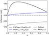Fig. 5. Difference between the velocity perturbation caused by an example radial p-mode (l = 0, n = 20, ωnl/2π = 2.90 mHz) of amplitude 1.0 m/s (at the surface at the disk center) computed from the HMI algorithm (without background velocity) and a simple line-of-sight approximation evaluated at the formation height at each position on the disk, hμ, or at disk center, hμ = 1. We note that δvlos is purely imaginary so that Re[δvth] and Re[δvgeom] are a deviation from the simple line-of-sight approximation. A center-to-limb effect is observed in the imaginary part and in the thermodynamic contribution. For this radial mode, the geometrical component is small.

Another contribution due to the structural changes (mostly temperature) causes a non-zero real part. This term modifies the shape of the line symmetrically compared to the central wavelength and should thus not contribute to the velocity. This, unfortunately, is not the case, as the filters and the line shape (not considered in this study) are not symmetric. This thermodynamical contribution causes a systematic phase shift with non-trivial center-to-limb variations, as it is out of phase compared to δv_line.

5.2. Velocity perturbation caused by high-degree modes

Figure 6 shows the perturbed velocity caused by a p-mode with l = 100 and n = 6 corresponding to a frequency of 2.93 mHz and an f-mode with l = 600 (frequency 2.45 mHz). As observed for the radial mode, the error due to the formation height increases toward the limb. This error also increases with the harmonic degree. The geometrical contributions also increase with the harmonic degree but remain relatively small. As expected, the thermodynamic effect vanishes for the f-mode. Overall, for all modes, the thermodynamic and/or geometrical contributions that are out of phase with the Doppler contributions cause systematic center-to-limb phase shifts. We note that these contributions vanish if we artificially symmetrize the HMI filters around the central wavelength (for a given background velocity). They are therefore caused by the shift of the line due to the background velocity resulting in asymmetric filters with respect to the HMI central wavelength. The (instrumental) asymmetry of the filters (and eventually of the line shape) also contributes to this phase shift.

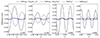Fig. 6. Same as Fig. 5 but for an example of the high-degree p-mode (l = 100, n = 6, ωnl/2π = 2.93 mHz) and the f-mode (l = 600, n = 0, ωnl/2π = 2.45 mHz) centered around μ = 0.2 and μ = 0.5 on the central meridian.

5.3. Modeling on the CCD with realistic background velocities

To get closer to the observations, we modeled the Doppler velocity on the CCD as it would be observed by HMI and included the effects of background velocities, in particular the satellite velocity and differential rotation. This was done to study the impact of background velocities on the evaluation of the perturbed velocities.

We denote by (x, y) the pixel coordinates on the CCD. We took into account the B₀- and P₀-angles in order to make the connection between the CCD coordinates (x, y) and the heliographic angles (θ, ϕ). To do so, we used the relations between pseudo-angles and the gnomonic (TAN) projection as described in Sect. 7.2 of Thompson (2006). The different values required to make the conversions were directly read from the HMI header.

We also included the satellite velocity associated with a given time frame by reading the keywords OBS_VW, OBS_VN, and OBS_VR from the HMI header. The background velocity is the sum of the line-of-sight projection of the Solar Dynamics Observatory motion (see for example Eq. 4 in Schuck et al. 2016) and the differential rotation given by

$$\begin{array}{c}\hfill {\mathrm{v}}_{\mathrm{los}}^{\mathrm{rot}}(\theta ,\varphi )={\mathbf{u}}^{\mathrm{rot}}·{\mathrm{e}}_{\mathrm{obs}}=-R_{\odot }\mathrm{\Omega }(\theta )sin\theta cos{B}_{0}sin\varphi .\end{array}$$(41)

We used a three-term approximation of the surface solar differential rotation Ω(θ)/2π = [454 − 55cos²θ − 76cos⁴θ] nHz.

A representation of the background velocity for a particular frame on June 6, 2011, at 00:00 is shown in the left panel of Fig. 7. This day was chosen because the B₀-angle is small. In this frame, the background velocity varies between 0 and 4 km/s, with the smallest values toward the east, where the satellite motion almost compensates for the rotation. Additional background flows such as convective blue shift and gravitational red shift could be added within this framework.

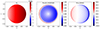Fig. 7. Effect of background velocity on the perturbed velocity caused by an example radial mode (l = 0, n = 20, ωnl/2π = 2.90 mHz) on June 6, 2011, at 00:00 when the B0 angle is close to 0. The left panel shows the line-of-sight component of the background velocity due to the satellite motion and solar differential rotation. The middle panel shows the amplitude (normalized by μ0), and the right panel corresponds to the phase (in degrees) of the perturbed velocity computed using the HMI algorithm. An animation over one day of observation is available online, and it illustrates the variations caused by the changing spacecraft motion.

The middle and right panels of Fig. 7 show the normalized amplitude (δv_HMI/μ₀) and the phase of the perturbed velocity caused by a radial mode. Such phase maps are often used to study systematics (see for example Couvidat et al. 2016). They are computed on a CCD grid with 300 pixels uniformly distributed in the x- and y-directions. From a simple line-of-sight velocity projection, the amplitude should be constant and equal to one over the disk, and the phase should be −90°. The variations in amplitude over the disk are mostly due to the Doppler shift term δv_line and depend on the center-to-limb distance. However, these variations also depend on the background velocity (see also the online animation associated with Fig. 7 showing the 24-hour variations of these quantities). The phase is mostly created by the thermodynamical contributions (the geometrical part is about one order of magnitude smaller but becomes more significant for higher-degree modes) and is anticorrelated with the background rotation with a Pearson correlation coefficient of −0.8. We note that the imaginary part of δv_HMI is almost completely anticorrelated with the rotation (correlation coefficient of −0.98).

6. HMI continuum intensity

The continuum intensity derived from the HMI algorithm (hmi.Ic_45s) is underestimated in the quiet Sun (Couvidat et al. 2012a). This underestimation arises from the imperfections of the HMI algorithm, which assumes a Gaussian line profile and employs non-ideal δ-function filters. These limitations lead to inaccurate discrete approximations of Fourier coefficients. Furthermore, the Doppler effect caused by the Solar and Dynamics Observatory’s motion around the Earth and the Sun results in a shift of the spectral line with respect to the HMI filters, contributing differently to each filtergram.

Figure 8 shows the perturbed continuum intensity as computed by the HMI algorithm for a radial p-mode (l = 0, n = 20, ω_nl/2π = 2.90 mHz). As was already noted for the theoretical continuum, the intensity depends on the distance to the disk center (Toutain et al. 1999; Kostogryz et al. 2021). However, the HMI continuum differs from the theoretical one by more than 10% depending on the position on the disk. Both the phase and the amplitude are affected with non-trivial variations across the detector. The thermodynamic contributions are mostly responsible for the amplitude variations, while the phase is linked to the imaginary contribution due to the line shift.

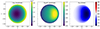Fig. 8. Continuum intensity perturbation caused by a radial p-mode (l = 0, n = 20, ωnl/2π = 2.90 mHz) on June 6, 2011, at 00:00. The amplitude (left) and phase (right) of the perturbed intensity were computed using the HMI algorithm. The middle panel shows the ratio between HMI and the theoretical continuum. An animation over one day of observation is available online.

7. Summary and discussion

In this paper, we have outlined the steps required to compute the perturbations in continuum intensity and Doppler velocity caused by oscillations of the solar surface. We found that approximating hmi.Ic_45s by the theoretical continuum and hmi.V_45s by a line-of-sight projection of the oscillations leads to an amplitude error of around 10% and a phase error of up to 10°. Due to the asymmetry of the filters with respect to the central wavelength (caused by background velocities as well as the filters themselves), hmi.V_45s is also influenced by thermodynamic perturbations (δv_th), while oscillation velocities (δv_line) also contribute to hmi.Ic_45s. A polynomial correction was implemented in the HMI pipeline to take into account the background velocities (Couvidat et al. 2016), and the quality of this correction can be assessed using the tools developed in this paper. Other sources of background velocities, such as convective blue shift and gravitational red shift (see for example Beckers & Nelson 1978) should be added to the background velocity before comparing perturbed quantities to observations.

More generally, the framework developed here can be used to gain insight into the systematic errors reported in the different helioseismic analyses. Notably, better understanding of these errors can allow for the use of additional measurements, such as the frequency-filtered travel times from Rajaguru et al. (2020) or the multi-height measurements proposed by Nagashima et al. (2014). However, we note that this framework cannot explain (instrumental) long-term variations, such as those observed in the travel times by Liang et al. (2018) (their Figure 4). The expressions for the perturbed intensity and velocity can also be used to construct improved leakage matrices (see for example Larson & Schou 2015) for global helioseismology or normal-mode coupling.

The framework has been illustrated on HMI but can be applied to other instruments, such as PHI and PMI. By shifting the spectral line to the Ni I 6768 line and adapting the algorithms, the data from MDI and GONG can also be analyzed, allowing for a comparison of systematic errors between the different instruments.

Data availability

Movies associated to Figs. 7 and 8 are available at https://www.aanda.org

Acknowledgments

We thank Philip Scherrer and Todd Hoeksema for useful discussions about the HMI algorithm and HMI observables, the provision of example HMI filters, and comments on the manuscript draft. We thank Zhi-Chao Liang for help with HMI keywords and the projection algorithm, as well as Aaron Birch and Ha Pham for comments on an earlier version of this manuscript. NK and LG acknowledge generous support from the German Aerospace Center (DLR) under grants “PLATO Data Center” 50OO1501 and 50OP1902. DF and LG acknowledge partial support from ERC Synergy grant WHOLE SUN 810218, from DFG grant SFB 1456 “Mathematics of Experiments” (project C04), and from DFG grant “Stellare Schmetterlingsdiagramme” no. 530101854. VW and AIS acknowledge support from ERC Synergy Grant REVEAL under the European Union’s Horizon 2020 research and innovation program (grant no. 101118581) IM acknowledges the financial support from the Serbian Ministry of Science and Technology through the grants 451-03-136/2025-03/200104 and 451-03-136/2025-03/200002.

References

Appendix A: Validation

This appendix shows the validation of the computation of perturbed continuum intensity and velocity. To do so, we compute the intensity at each wavelength in a background model characterized by (r₀, p₀, T₀, u = 0) and perturbed intensities. The perturbed intensities are computed with a media characterized by (r₀, p, T, u = 0) for δI_th, (r₀e_r + ξ, p₀, T₀, u = 0) for δI_geom, and (r₀, p₀, T₀, d_tξ) for δI_line.

A validation of the intensity as a function of wavelength is shown in the main text in Fig. 4. Here, we additionally compare the perturbed continuum intensity in Fig. A.1 and velocity in Fig. A.2. The direct and first-order computations agree well. For velocity computations, the main contribution is coming as expected from the line shift (that is the term δI_line) but small deviation due to the thermodynamic term is observed in particular for small values of μ. Such a deviation could introduce systematic effects in the interpretation of the observables.

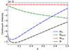Fig. A.1. Test of the direct computation of continuum intensity (dots) as a function μ and comparison with the first-order computation (solid line). The thermodynamical, geometrical, and line contributions are represented separately in blue, green, and red respectively while the full intensity is in black. The wavelength offset is with respect to the center of the HMI line λHMI = 6173.33 Å.

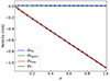Fig. A.2. Test of the direct computation of velocity and comparison with the first-order computation. The velocity computation is done with the HMI algorithm after convolution of the intensity with the filtergrams shown in Fig. 2. The different contributions as well as the total velocity are shown using the first-order approach (solid line) and direct computation (dots).

Appendix B: Look-up tables

The look-up table gives the correspondence between the velocity computed from the HMI algorithm and the real Doppler velocity

$$\begin{array}{c}\hfill {\mathrm{v}}_{\mathrm{HMI}}^0={\mathcal{F}}_{\mathrm{HMI}}({\mathrm{v}}^0,{\mu }_0).\end{array}$$(B.1)

To obtain ℱ_HMI, we manually shift the line of a given wavelength Δλ corresponding to a Doppler shift of Δλ c/λ and compare this shift to v_HMI⁰ using the HMI algorithm. A representation of this function at the disk center is given on the left panel of Fig. B.1. As the filters are not symmetric, an offset is visible between the velocity obtained by the algorithm and the real velocity. Otherwise, the slope is very close to 1 with some deviations only for very large background velocities (larger than 6 km/s).

To compute the perturbed velocity, we also need the derivatives of the look-up table with respect to v⁰ and μ₀ as

$$\begin{array}{c}\hfill \delta {\mathrm{v}}_{\mathrm{HMI}}=\delta \mathrm{v}\frac{\partial {\mathcal{F}}_{\mathrm{HMI}}}{\partial {\mathrm{v}}^0}+\delta \mu \frac{\partial {\mathcal{F}}_{\mathrm{HMI}}}{\partial {\mu }_0}.\end{array}$$(B.2)

A representation of these two derivatives is shown in Fig. B.1. For small background velocities $\frac{\partial {\mathcal{F}}_{\mathrm{HMI}}}{\partial {\text{v}}^0}\approx 1$ and $\frac{\partial {\mathcal{F}}_{\mathrm{HMI}}}{\partial {\mu }_0}\approx 0$ so that δv_HMI ≈ δv. However, some strong deviations appear for large background velocities which could lead to an underestimation of the real velocity (as $\frac{\partial {\mathcal{F}}_{\mathrm{HMI}}}{\partial {\text{v}}^0}>1$) but also to some variations depending on the distance to the disk center when $\frac{\partial {\mathcal{F}}_{\mathrm{HMI}}}{\partial {\mu }_0}$ is significant.

To show the importance of Eq. (B.2) in computing the perturbed velocity, we perturb the reference model by a function that is independent of depth (and varies with latitude as a Legendre polynomial of order 10). In this case, we know the exact value of the perturbed velocity and we can compare it to the value returned by the HMI algorithm with or without the look-up tables. Such a comparison is made in Fig. B.2. After taking the look-up table into account, the velocity δv_HMI perfectly matches the expected value. However, it deviates from the value without applying the look-up table, in particular for very large background velocities. We note finally that the correction due to the term $\delta \mu \frac{\partial {\mathcal{F}}_{\mathrm{HMI}}}{\partial {\mu }_0}$ is very small (5 order of magnitude smaller than the other term in this case).

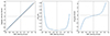Fig. B.1. Look-up table and derivatives at μ = 1 necessary to map the HMI velocity to real Doppler velocity. Left: ℱHMI (blue line) compared to the one-to-one correspondence (black). Middle: ∂ℱHMI/∂v0. Right: ∂ℱHMI/∂μ0. These two derivatives are necessary to compute the perturbed velocity.

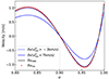Fig. B.2. Perturbed velocity computed with the HMI algorithm with and without applying the look-up table. For large background velocities, the amplitude correction due to the look-up table is significant. Note that δvHMI is the same for all background velocities.

Appendix C: First-order perturbations in velocity and intensity

In order to obtain the first-order perturbations in the different HMI observables, we decompose the Fourier coefficients a₁ and b₁ as

$$\begin{array}{c}\hfill a_1=a_1^0+\delta a_1\text{and}{b}_1=b_1^0+\delta b_1,\end{array}$$(C.1)

where a₁⁰ and b₁⁰ (resp. δa₁ and δb₁) are computed from Eqs. (7) and (8) using the background intensity ℐ_j⁰ (resp. perturbed intensities δℐ_j).

C.1. Velocity

From the velocity definition (Eq. (9)), we obtained

$$\begin{array}{c}\hfill \mathrm{v}=V_{\mathrm{dop}}arctan\left(\frac{b_1^0+\delta b_1}{a_1^0+\delta a_1}\right)=V_{\mathrm{dop}}arctan(\frac{b_1^0}{a_1^0}+\frac{\delta b_1}{a_1^0}-\frac{\delta a_1{b}_1^0}{{(a_1^0)}^2}).\end{array}$$(C.2)

We used a first-order development of the arctan

$$\begin{array}{c}\hfill arctan(x+ϵ)=arctanx+\frac{ϵ}{1+x^2},\end{array}$$(C.3)

to obtain v = v⁰ + δv, where

$$\begin{array}{cc}\hfill {\mathrm{v}}^0& =V_{\mathrm{dop}}arctan\left(\frac{b_1^0}{a_1^0}\right),\hfill \end{array}$$(C.4)

$$\begin{array}{cc}\hfill \delta \mathrm{v}& =V_{\mathrm{dop}}\frac{a_1^0\delta b_1-b_1^0\delta a_1}{{(a_1^0)}^2+{(b_1^0)}^2}.\hfill \end{array}$$(C.5)

By replacing the expressions of the Fourier coefficients, δv can also be written as

$$\begin{array}{c}\hfill \delta \mathrm{v}=V_{\mathrm{dop}}\frac{{\displaystyle {\sum }_{i,j}}{\mathcal{I}}_i^0\delta {\mathcal{I}}_{j}sin\left(2\pi \frac{j-i}{N}\right)}{{\displaystyle {\sum }_{i,j}}{\mathcal{I}}_i^0{\mathcal{I}}_j^{0}cos\left(2\pi \frac{j-i}{N}\right)}.\end{array}$$(C.6)

C.2. Line width

Using the first-order perturbation of the Fourier coefficients, the line width σ is rewritten as

$$\begin{array}{cc}\hfill \sigma & :=\frac{T}{\pi \sqrt{6}}\sqrt{log\left(\frac{a_1^2+b_1^2}{a_2^2+b_2^2}\right)}=\frac{T}{\pi \sqrt{6}}\sqrt{log[{(a_1^0)}^2+{(b_1^0)}^2+2a_1^0\delta a_1+2b_1^0\delta b_1]-log[{(a_2^0)}^2+{(b_2^0)}^2+2a_2^0\delta a_2+2b_2^0\delta b_2]},\hfill \end{array}$$(C.7)

$$\begin{array}{cc}& =\frac{T}{\pi \sqrt{6}}\sqrt{log[{(a_1^0)}^2+{(b_1^0)}^2]+2\frac{a_1^0\delta a_1+b_1^0\delta b_1}{{(a_1^0)}^2+{(b_1^0)}^2}-log[{(a_2^0)}^2+{(b_2^0)}^2]-2\frac{a_2^0\delta a_2+b_2^0\delta b_2}{{(a_2^0)}^2+{(b_2^0)}^2}}.\hfill \end{array}$$(C.8)

We obtained σ = σ₀ + δσ where the perturbation to the line width δσ is given by

$$\begin{array}{c}\hfill \delta \sigma =\frac{T^2}{6{\pi }^2{\sigma }_0}[\frac{a_1^0\delta a_1+b_1^0\delta b_1}{{(a_1^0)}^2+{(b_1^0)}^2}-\frac{a_2^0\delta a_2+b_2^0\delta b_2}{{(a_2^0)}^2+{(b_2^0)}^2}].\end{array}$$(C.9)

C.3. Line depth

The line depth I_d is developed at first order as

$$\begin{array}{cc}\hfill I_d& =\frac{T}{2\sqrt{\pi }\sigma }\sqrt{a_1^2+b_1^2}exp\left(\frac{{\pi }^2{\sigma }^2}{T^2}\right)=\frac{T}{2\sqrt{\pi }({\sigma }_0+\delta \sigma )}\sqrt{{(a_1^0)}^2+{(b_1^0)}^2+2\delta a_1{a}_1^0+2\delta b_1{b}_1^0}exp\left(\frac{{\pi }^2({\sigma }_0^2+2{\sigma }_0\delta \sigma )}{T^2}\right),\hfill \end{array}$$(C.10)

$$\begin{array}{cc}& =\frac{T}{2\sqrt{\pi }{\sigma }_0}[(1-\frac{\delta \sigma }{{\sigma }_0})\sqrt{{(a_1^0)}^2+{(b_1^0)}^2}(1+\frac{\delta a_1{a}_1^0+\delta b_1{b}_1^0}{{(a_1^0)}^2+{(b_1^0)}^2})exp\left(\frac{{\pi }^2{\sigma }_0^2}{T^2}\right)(1+\frac{2{\pi }^2}{T^2}{\sigma }_0\delta \sigma )]=I_d^0+\delta I_d,\hfill \end{array}$$(C.11)

where

$$\begin{array}{c}\hfill \delta I_d=I_d^0[-\frac{\delta \sigma }{{\sigma }_0}+\frac{\delta a_1{a}_1^0+\delta b_1{b}_1^0}{{(a_1^0)}^2+{(b_1^0)}^2}+\frac{2{\pi }^2{\sigma }_0\delta \sigma }{T^2}],\end{array}$$(C.12)

and δσ is given by Eq. (C.9).

C.4. Continuum intensity

Using the previously derived expressions for the perturbed line width δσ and line depth δI_d, we can compute the perturbed continuum intensity

$$\begin{array}{cc}\hfill I_{\mathrm{HMI}}& =\frac{1}{N}{\displaystyle \sum _{j=1}^N}[I_j+I_d\text{exp}(-\frac{{({\lambda }_j-{\lambda }_{\mathrm{HMI}})}^2}{{\sigma }^2})]=\frac{1}{6}{\displaystyle \sum _{j=1}^N}[I_j^0+\delta I_j+(I_d^0+\delta I_d)\text{exp}(-\frac{{({\lambda }_j-{\lambda }_{\mathrm{HMI}})}^2}{{\sigma }_0^2+2{\sigma }_0\delta \sigma })],\hfill \end{array}$$(C.13)

$$\begin{array}{cc}& =\frac{1}{N}{\displaystyle \sum _{j=1}^N}[I_j^0+\delta I_j+(I_d^0+\delta I_d)\text{exp}(-\frac{{({\lambda }_j-{\lambda }_{\mathrm{HMI}})}^2}{{\sigma }_0^2})(1+2\frac{{({\lambda }_j-{\lambda }_{\mathrm{HMI}})}^2}{{\sigma }_0^2}\frac{\delta \sigma }{{\sigma }_0})],\hfill \end{array}$$(C.14)

$$\begin{array}{cc}& =I_{\mathrm{HMI}}^0+\frac{1}{N}{\displaystyle \sum _{j=1}^N}[\delta I_j+\delta I_d\text{exp}(-\frac{{({\lambda }_j-{\lambda }_{\mathrm{HMI}})}^2}{{\sigma }_0^2})]+I_d^0\frac{\delta \sigma }{{\sigma }_0}\frac{2}{N}{\displaystyle \sum _{j=1}^N}\text{exp}(-\frac{{({\lambda }_j-{\lambda }_{\mathrm{HMI}})}^2}{{\sigma }_0^2})\frac{{({\lambda }_j-{\lambda }_{\mathrm{HMI}})}^2}{{\sigma }_0^2}=I_{\mathrm{HMI}}^0+\delta I_{\mathrm{HMI}},\hfill \end{array}$$(C.15)

where

$$\begin{array}{c}\hfill \delta I_{\mathrm{HMI}}=\frac{1}{N}{\displaystyle \sum _{j=1}^N}[\delta {\mathcal{I}}_j+exp(-\frac{{({\lambda }_j-{\lambda }_{\mathrm{HMI}})}^2}{{\sigma }_0^2})(\delta I_d+2I_d^0\frac{\delta \sigma }{{\sigma }_0}\frac{{({\lambda }_j-{\lambda }_{\mathrm{HMI}})}^2}{{\sigma }_0^2})].\end{array}$$(C.16)

Appendix D: Rewriting the thermodynamical contributions

We have shown in K+21 that

$$\begin{array}{c}\hfill \delta I_{\tau ,\alpha }={\displaystyle {\int }_0^{{\tau }^{\max }}}{S}_{\lambda }^0{\text{e}}^{-{\tau }_{\lambda }^0/{\mu }_0}(\frac{\delta {\alpha }_{\lambda }}{{\alpha }_{\lambda }^0}-{\displaystyle {\int }_0^{{\tau }_{\lambda }^0}\frac{\delta {\alpha }_{\lambda }}{{\alpha }_{\lambda }^0}\frac{d{\tau }_{\lambda }^{\prime }}{{\mu }_0}})\frac{d{\tau }_{\lambda }^0}{{\mu }_0}.\end{array}$$(D.1)

Here, we give an equivalent form in order to make appear the background intensity I_λ⁰. The second term can be integrated by part

$$\begin{array}{cc}\hfill {\displaystyle {\int }_0^{{\tau }^{\max }}}{S}_{\lambda }^0{\text{e}}^{-{\tau }_{\lambda }^0/{\mu }_0}{\displaystyle {\int }_0^{{\tau }_{\lambda }^0}\frac{\delta {\alpha }_{\lambda }}{{\alpha }_{\lambda }^0}\frac{d{\tau }_{\lambda }^{\prime }}{{\mu }_0}\frac{d{\tau }_{\lambda }^0}{{\mu }_0}}& =-{\displaystyle {\int }_0^{{\tau }^{\max }}}\left[{\displaystyle {\int }_0^{{\tau }_{\lambda }^0}{S}_{\lambda }^0{\text{e}}^{-{\tau }_{\lambda }^{\prime }/{\mu }_0}\frac{d{\tau }_{\lambda }^{\prime }}{{\mu }_0}}\right]\frac{\delta {\alpha }_{\lambda }}{{\alpha }_{\lambda }^0}\frac{d{\tau }_{\lambda }^0}{{\mu }_0}+{\displaystyle {\int }_0^{{\tau }^{\max }}}{S}_{\lambda }^0{\text{e}}^{-{\tau }_{\lambda }^0/{\mu }_0}\frac{d{\tau }_{\lambda }^0}{{\mu }_0}{\displaystyle {\int }_0^{{\tau }^{\max }}}\frac{\delta {\alpha }_{\lambda }}{{\alpha }_{\lambda }^0}\frac{d{\tau }_{\lambda }^0}{{\mu }_0},\hfill \end{array}$$(D.2)

$$\begin{array}{cc}& =-{\displaystyle {\int }_0^{{\tau }^{\max }}}[I_{\lambda }^0(0,{\mu }_0)-{\displaystyle {\int }_{{\tau }_{\lambda }^0}^{{\tau }^{\max }}{S}_{\lambda }^0{\text{e}}^{-{\tau }_{\lambda }^{\prime }/{\mu }_0}}\frac{d{\tau }_{\lambda }^{\prime }}{{\mu }_0}]\frac{\delta {\alpha }_{\lambda }}{{\alpha }_{\lambda }^0}\frac{d{\tau }_{\lambda }^0}{{\mu }_0}+I_{\lambda }^0(0,{\mu }_0){\displaystyle {\int }_0^{{\tau }^{\max }}}\frac{\delta {\alpha }_{\lambda }}{{\alpha }_{\lambda }^0}\frac{d{\tau }_{\lambda }^0}{{\mu }_0},\hfill \end{array}$$(D.3)

$$\begin{array}{cc}& ={\text{e}}^{-{\tau }_{\lambda }^0/{\mu }_0}{\displaystyle {\int }_0^{{\tau }^{\max }}}{I}_{\lambda }^0({\tau }_{\lambda }^0,{\mu }_0)\frac{\delta {\alpha }_{\lambda }}{{\alpha }_{\lambda }^0}\frac{d{\tau }_{\lambda }^0}{{\mu }_0}.\hfill \end{array}$$(D.4)

Thus

$$\begin{array}{c}\hfill \delta I_{\tau ,\alpha }={\displaystyle {\int }_0^{{\tau }^{\max }}}[S_{\lambda }^0-I_{\lambda }^0({\tau }_{\lambda }^0,{\mu }_0)]{\text{e}}^{-{\tau }_{\lambda }^0/{\mu }_0}\frac{\delta {\alpha }_{\lambda }}{{\alpha }_{\lambda }^0}\frac{d{\tau }_{\lambda }^0}{{\mu }_0},\end{array}$$(D.5)

a form already obtained by Zhugzhda et al. (1996).

All Tables

All Figures

	Fig. 1. Background sound speed (red) and density (blue) from Model S (dashed), MPS-ATLAS (solid), and the patched model used in this study (dots). The gray region represents the domain where the patching between Model S and MPS-ATLAS is done. The zero level of height in this context is defined at one solar radius.
In the text

Fig. 2. Background intensity computed from the MPS-ATLAS solar model atmosphere (solid), the standard solar Model S (dashed), and from the observations (dots). Left: Limb darkening (Ic(μ)/Ic(μ = 1)) in the continuum around the HMI line compared with the observations from Neckel & Labs (1994). Right: Synthesized FeI spectral line background intensity ($\stackrel{\sim }{I}(\lambda ,\mu )/I_c(\mu =1)$) compared with the observations from the IAG spectral atlas (Ellwarth et al. 2023) at μ = 1 (blue) and μ = 0.5 (red). The wavelength offset is with respect to the center of the HMI line λHMI = 6173.33 Å. The black dashed curves represent the six HMI filtergrams.

In the text

	Fig. 3. Response function for velocity K(s, μ) (in Mm−1) defined by Eq. (34) as a function of height, s, and limb angle, μ. The black and white lines respectively represent the maximum and center of gravity of the response function for each value of μ.
In the text

	Fig. 4. Test of the direct computation of the perturbed intensity (Iλ − Iλ0)/Iλ0 (dots) for μ = 0.5 and comparison with first-order computations δIλ/Iλ0 (solid line). The thermodynamic, geometrical, and line contributions are represented separately in blue, green, and red, while the full intensity is in black. The wavelength offset is with respect to the center of the HMI line λHMI = 6173.33 Å.
In the text

Fig. 5. Difference between the velocity perturbation caused by an example radial p-mode (l = 0, n = 20, ωnl/2π = 2.90 mHz) of amplitude 1.0 m/s (at the surface at the disk center) computed from the HMI algorithm (without background velocity) and a simple line-of-sight approximation evaluated at the formation height at each position on the disk, hμ, or at disk center, hμ = 1. We note that δvlos is purely imaginary so that Re[δvth] and Re[δvgeom] are a deviation from the simple line-of-sight approximation. A center-to-limb effect is observed in the imaginary part and in the thermodynamic contribution. For this radial mode, the geometrical component is small.

In the text

	Fig. 6. Same as Fig. 5 but for an example of the high-degree p-mode (l = 100, n = 6, ωnl/2π = 2.93 mHz) and the f-mode (l = 600, n = 0, ωnl/2π = 2.45 mHz) centered around μ = 0.2 and μ = 0.5 on the central meridian.
In the text

Fig. 7. Effect of background velocity on the perturbed velocity caused by an example radial mode (l = 0, n = 20, ωnl/2π = 2.90 mHz) on June 6, 2011, at 00:00 when the B0 angle is close to 0. The left panel shows the line-of-sight component of the background velocity due to the satellite motion and solar differential rotation. The middle panel shows the amplitude (normalized by μ0), and the right panel corresponds to the phase (in degrees) of the perturbed velocity computed using the HMI algorithm. An animation over one day of observation is available online, and it illustrates the variations caused by the changing spacecraft motion.

In the text

	Fig. 8. Continuum intensity perturbation caused by a radial p-mode (l = 0, n = 20, ωnl/2π = 2.90 mHz) on June 6, 2011, at 00:00. The amplitude (left) and phase (right) of the perturbed intensity were computed using the HMI algorithm. The middle panel shows the ratio between HMI and the theoretical continuum. An animation over one day of observation is available online.
In the text

	Fig. A.1. Test of the direct computation of continuum intensity (dots) as a function μ and comparison with the first-order computation (solid line). The thermodynamical, geometrical, and line contributions are represented separately in blue, green, and red respectively while the full intensity is in black. The wavelength offset is with respect to the center of the HMI line λHMI = 6173.33 Å.
In the text

	Fig. A.2. Test of the direct computation of velocity and comparison with the first-order computation. The velocity computation is done with the HMI algorithm after convolution of the intensity with the filtergrams shown in Fig. 2. The different contributions as well as the total velocity are shown using the first-order approach (solid line) and direct computation (dots).
In the text

	Fig. B.1. Look-up table and derivatives at μ = 1 necessary to map the HMI velocity to real Doppler velocity. Left: ℱHMI (blue line) compared to the one-to-one correspondence (black). Middle: ∂ℱHMI/∂v0. Right: ∂ℱHMI/∂μ0. These two derivatives are necessary to compute the perturbed velocity.
In the text

	Fig. B.2. Perturbed velocity computed with the HMI algorithm with and without applying the look-up table. For large background velocities, the amplitude correction due to the look-up table is significant. Note that δvHMI is the same for all background velocities.
In the text

References

- Agrawal, P., Rast, M. P., & Ruiz Cobo, B. 2023, ApJ, 944, 111 [Google Scholar]
- Asplund, M., Grevesse, N., Sauval, A. J., & Scott, P. 2009, ARA&A, 47, 481 [NASA ADS] [CrossRef] [Google Scholar]
- Beckers, J. M., & Milkey, R. W. 1975, Sol. Phys., 43, 289 [Google Scholar]
- Beckers, J. M., & Nelson, G. D. 1978, Sol. Phys., 58, 243 [NASA ADS] [CrossRef] [Google Scholar]
- Bogart, R. S., Baldner, C. S., & Basu, S. 2015, ApJ, 807, 125 [NASA ADS] [CrossRef] [Google Scholar]
- Cavallini, F. 2006, Sol. Phys., 236, 415 [NASA ADS] [CrossRef] [Google Scholar]
- Christensen-Dalsgaard, J., Däppen, W., Ajukov, S. V., et al. 1996, Science, 272, 1286 [Google Scholar]
- Couvidat, S., Rajaguru, S. P., Wachter, R., et al. 2012a, Sol. Phys., 278, 217 [NASA ADS] [CrossRef] [Google Scholar]
- Couvidat, S., Schou, J., Shine, R. A., et al. 2012b, Sol. Phys., 275, 285 [NASA ADS] [CrossRef] [Google Scholar]
- Couvidat, S., Schou, J., Hoeksema, J. T., et al. 2016, Sol. Phys., 291, 1887 [Google Scholar]
- Ellwarth, M., Schäfer, S., Reiners, A., & Zechmeister, M. 2023, A&A, 673, A19 [NASA ADS] [CrossRef] [EDP Sciences] [Google Scholar]
- Fleck, B., Couvidat, S., & Straus, T. 2011, Sol. Phys., 271, 27 [Google Scholar]
- Gray, D. F. 2021, The Observation and Analysis of Stellar Photospheres (Cambridge University Press) [Google Scholar]
- Kostogryz, N. M., Fournier, D., & Gizon, L. 2021, A&A, 654, A1 (K+21) [Google Scholar]
- Kostogryz, N. M., Witzke, V., Shapiro, A. I., et al. 2022, A&A, 666, A60 [NASA ADS] [CrossRef] [EDP Sciences] [Google Scholar]
- Kupka, F., Piskunov, N., Ryabchikova, T. A., Stempels, H. C., & Weiss, W. W. 1999, A&AS, 138, 119 [NASA ADS] [CrossRef] [EDP Sciences] [Google Scholar]
- Landi Degl’Innocenti, E., & Landi Degl’Innocenti, M. 1977, A&A, 56, 111 [NASA ADS] [Google Scholar]
- Larson, T. P., & Schou, J. 2015, Sol. Phys., 290, 3221 [NASA ADS] [CrossRef] [Google Scholar]
- Liang, Z.-C., Gizon, L., Birch, A. C., Duvall, T. L., & Rajaguru, S. P. 2018, A&A, 619, A99 [NASA ADS] [CrossRef] [EDP Sciences] [Google Scholar]
- Milić, I., & van Noort, M. 2017, A&A, 601, A100 [NASA ADS] [CrossRef] [EDP Sciences] [Google Scholar]
- Nagashima, K., Löptien, B., Gizon, L., et al. 2014, Sol. Phys., 289, 3457 [Google Scholar]
- Neckel, H., & Labs, D. 1994, Sol. Phys., 153, 91 [CrossRef] [Google Scholar]
- Petrie, G. J. D., Blanco Rodríguez, J., Martínez Pillet, V., Uitenbroek, H., & Scherrer, P. H. 2025, ApJS, 278, 55 [Google Scholar]
- Piskunov, N. E., Kupka, F., Ryabchikova, T. A., Weiss, W. W., & Jeffery, C. S. 1995, A&AS, 112, 525 [Google Scholar]
- Rajaguru, S. P., & Antia, H. M. 2020, in Dynamics of the Sun and Stars; Honoring the Life and Work of Michael J. Thompson, eds. M. J. P. F. G. Monteiro, R. A. García, J. Christensen-Dalsgaard, & S. W. McIntosh, Astrophys. Space Sci. Proc., 57, 107 [Google Scholar]
- Ryabchikova, T., Piskunov, N., Kurucz, R. L., et al. 2015, Phys. Scr, 90, 054005 [Google Scholar]
- Scharmer, G. B., Langhans, K., Kiselman, D., & Löfdahl, M. G. 2007, in New Solar Physics with Solar-B Mission, eds. K. Shibata, S. Nagata, & T. Sakurai, ASP Conf. Ser., 369, 71 [Google Scholar]
- Scherrer, P. H., Bogart, R. S., Bush, R. I., et al. 1995, Sol. Phys., 162, 129 [Google Scholar]
- Schuck, P. W., Antiochos, S. K., Leka, K. D., & Barnes, G. 2016, ApJ, 823, 101 [NASA ADS] [CrossRef] [Google Scholar]
- Solanki, S. K., del Toro Iniesta, J. C., Woch, J., et al. 2020, A&A, 642, A11 [NASA ADS] [CrossRef] [EDP Sciences] [Google Scholar]
- Staub, J., Fernandez-Rico, G., Gandorfer, A., et al. 2020, J. Space Weather Space Clim., 10, 54 [NASA ADS] [CrossRef] [EDP Sciences] [Google Scholar]
- Takeda, Y., & UeNo, S. 2019, Sol. Phys., 294, 63 [NASA ADS] [CrossRef] [Google Scholar]
- Thompson, W. T. 2006, A&A, 449, 791 [NASA ADS] [CrossRef] [EDP Sciences] [Google Scholar]
- Toutain, T., & Gouttebroze, P. 1993, A&A, 268, 309 [NASA ADS] [Google Scholar]
- Toutain, T., Berthomieu, G., & Provost, J. 1999, A&A, 344, 188 [NASA ADS] [Google Scholar]
- Townsend, R. H. D., & Teitler, S. A. 2013, MNRAS, 435, 3406 [Google Scholar]
- Vukadinović, D., Milić, I., & Atanacković, O. 2022, A&A, 664, A182 [NASA ADS] [CrossRef] [EDP Sciences] [Google Scholar]
- Witzke, V., Shapiro, A. I., Cernetic, M., et al. 2021, A&A, 653, A65 [NASA ADS] [CrossRef] [EDP Sciences] [Google Scholar]
- Zhugzhda, Y. D., Staude, J., & Bartling, G. 1996, A&A, 305, L33 [Google Scholar]