| Issue |
A&A
Volume 703, November 2025
|
|
|---|---|---|
| Article Number | A226 | |
| Number of page(s) | 9 | |
| Section | Astrophysical processes | |
| DOI | https://doi.org/10.1051/0004-6361/202553812 | |
| Published online | 21 November 2025 | |
Studying the properties of reconnection-driven turbulence
1
School of Mathematics and Computational Sciences, Xiangtan University, Xiangtan, Hunan 411105, People’s Republic of China
2
Department of Physics, Xiangtan University, Xiangtan, Hunan 411105, People’s Republic of China
3
Key Laboratory of Stars and Interstellar Medium, Xiangtan University, Xiangtan 411105, People’s Republic of China
4
Hunan Key Laboratory for Computation and Simulation in Science and Engineering, Xiangtan 411105, People’s Republic of China
5
Hunan National Center for Applied Mathematics, Xiangtan 411105, People’s Republic of China
⋆ Corresponding authors: This email address is being protected from spambots. You need JavaScript enabled to view it.
; This email address is being protected from spambots. You need JavaScript enabled to view it.
Received:
20
January
2025
Accepted:
10
October
2025
Abstract
Context. Magnetic reconnection, often accompanied by a turbulence interaction, is a ubiquitous phenomenon in astrophysical environments. However, the current understanding of the nature of turbulent magnetic reconnection remains insufficient.
Aims. We investigate the statistical properties of reconnection turbulence in the framework of the self-driven reconnection.
Methods. Using the open-source software package AMUN, we first performed numerical simulations of turbulent magnetic reconnection. We then obtained the statistical results of reconnection turbulence by traditional statistical methods such as the power spectrum and structure function.
Results. Our numerical results demonstrate: (1) the velocity spectrum of reconnection turbulence follows the classical Kolmogorov type of E ∝ k−5/3, while the magnetic field spectrum is steeper than the Kolmogorov spectrum, which are independent of limited resistivity, guide field, and isothermal or adiabatic fluid states; (2) most of the simulations show the anisotropy cascade, except that the presence of a guide field leads to an isotropic cascade; (3) reconnection turbulence is incompressible in the adiabatic state, with energy distribution being dominated by the velocity solenoidal component; and (4) different from pure magnetohydrodynamic (MHD) turbulence, the intermittency of the velocity field is stronger than that of the magnetic field in reconnection turbulence.
Conclusions. The steep magnetic field spectrum, together with the velocity spectrum of a Kolmogorov type, can characterize the feature of the reconnection turbulence. In the case of the presence of the guide field, the isotropy of the reconnection turbulence cascade is also different from the cascade mode of pure MHD turbulence. Our experimental results provide new insights into the properties of reconnection turbulence, which will contribute to advancing self-driven reconnection theory.
Key words: acceleration of particles / turbulence / cosmic rays / ISM: magnetic fields / ISM: structure
© The Authors 2025
 Open Access article, published by EDP Sciences, under the terms of the Creative Commons Attribution License (https://creativecommons.org/licenses/by/4.0), which permits unrestricted use, distribution, and reproduction in any medium, provided the original work is properly cited.
This article is published in open access under the Subscribe to Open model. This email address is being protected from spambots. You need JavaScript enabled to view it. to support open access publication.
1. Introduction
Magnetic reconnection is a fundamental physical process that facilitates the conversion of magnetic energy into kinetic and internal energies. This phenomenon is prevalent in various astrophysical environments such as solar flares (Dere 1996; Chitta & Lazarian 2020; Li et al. 2024), pulsar wind nebulae (Meyer et al. 2010; Tavani et al. 2011), and gamma-ray bursts (Gehrels et al. 2009). Sweet (1958) and Parker (1957) developed a theoretical model, known as the Sweet-Parker model, to describe reconnection processes. In this model, the reconnection rate is determined by VR ∼ VA(Δ/L)∼VAS−1/2, where S = LVA/η represents the Lundquist number, VA the Alfvén velocity, L and Δ the length and thickness of the current sheet, as well as η the Ohmic resistivity. Given the high Lundquist number in the astrophysical environment, the Sweet-Parker model predicts a low reconnection rate, which contradicts the observations (see Dere 1996 for an example of fast-flare phenomena). To enhance the reconnection rate, Petschek (1964) proposed an X-type reconnection configuration (known as an X-point model), which converges magnetic field lines to the reconnection region at a sharp angle, resulting in L being so small that it is comparable to Δ. Currently, some observations (Shibata et al. 1995; Eriksson et al. 2004; Drake et al. 2006) and simulations (Lin & Forbes 2000; Wang et al. 2023) support this model. Meanwhile, a 2D Petschek-type standard flare model can also explain various macroscale flare characteristics of the Sun (Carmichael 1964; Sturrock 1966; Hirayama 1974; Kopp & Pneuman 1976). Although this structure can effectively enhance the reconnection rate, the main challenge is that this structure cannot be maintained on a large astrophysical scale, rapidly collapsing to the Sweet-Parker configuration, as found in magnetohydrodynamic (MHD) simulations (Biskamp 1996).
Given that the magnetic reconnection process is highly dynamic, Lazarian & Vishniac (1999, hereafter LV99) introduced turbulence to magnetic reconnection, inducing magnetic field wandering, to thicken the reconnection layer Δ. Since the wandering of the large-scale magnetic field directly determines the value of Δ, the LV99 theory found that the reconnection rate significantly depends on the turbulence level rather than the plasma resistivity. In the framework of the turbulent reconnection model, the fast reconnection rate is given by VR ≈ VAmin[(l/L)1/2, (L/l)1/2]MA2, where l is the scale of turbulent eddies. Naturally, for a trans-Alfvénic turbulence (MA ∼ 1), the reconnection rate ultimately reaches the Alfvén velocity VA on the system size. The 2D numerical testing of the LV99 model demonstrated that the reconnection rate still depends on the resistivity (Loureiro et al. 2009; Kulpa-Dybeł et al. 2010). Note that the LV99 model itself should be 3D in nature due to the 3D dynamic interactions of magnetic fields. By injecting turbulent flow into an antiparallel magnetic field using the external driving method, Kowal et al. (2009), Kowal (2012) performed the first 3D reconnection simulations to test the LV99 model and demonstrated that reconnection is indeed rapid in the presence of turbulence, as it is independent of resistivity. The reason for the difference between 2D and 3D numerical testing is that the 2D and 3D magnetized turbulence numerically exhibit distinct characteristics (Eyink et al. 2011). From the perspective of analytical analysis, Vishniac et al. (2012) predicted that turbulence within the reconnection region is similar to turbulence in a homogeneous system.
Turbulence can also be generated by the inhomogeneous current sheet caused by the presence of MHD instabilities, rendering the imposed external turbulence unnecessary, which is called self-driven (SD) reconnection (see LV99 and Lazarian & Vishniac 2009 for details). In the SD reconnection scenario, the inhomogeneity of the current sheet makes the current sheet thicker and the outflow stronger, leading to an increase in turbulence. The reconnection process facilitates turbulence interactions and increases the reconnection rate predicted in LV99. Subsequently, numerical simulations (Beresnyak 2017; Kowal et al. 2017) verified this theoretical prediction. In the case of incompressibility, Beresnyak (2017) numerically simulated the 3D case of SD reconnection, with the findings being the following: (1) unlike the 2D reconnection, the position of the current sheet changes with the evolution of the system in the 3D case; (2) the flux ropes observed in the 3D case are different from the 2D magnetic island exhibiting turbulence within its interior; and (3) the number of flux ropes is independent of the Lundquist number, in contrast to Uzdensky et al. (2010). Moreover, Beresnyak (2017) found that the power spectrum presents the power-law relationship of E(k)∝k−5/3, consistent with the She & Leveque (1995, hereafter GS95) theory.
In the case of the isothermal equation of state (EOS), Oishi et al. (2015) claimed a weak dependence of the width of the current sheet Δ on the resistivity η. However, they did not examine the properties of turbulence. Kowal et al. (2017) reported that the reconnection turbulence is similar to the pure MHD turbulence, though significantly affected by the flow dynamics induced by reconnection, especially in the low β region. Furthermore, Kowal et al. (2020) found that the tearing instability dominates the reconnection rate at the early stage. In contrast, when a sufficient turbulence amplitude is reached near the current sheet, the Kelvin-Helmholtz instability dominates turbulence generation over the tearing instability. In the case of the adiabatic EOS, Huang & Bhattacharjee (2016) found a nearly scale-independent anisotropy of the velocity fluctuations, with a slope in the range of −2.5 to −2.3, in contrast to the theoretical predictions of GS95. In the framework of SD reconnection, our recent work studied the dynamics of magnetic reconnection and the properties of acceleration of the test particle (Liang et al. 2023). We found that the power spectrum of the magnetic field exhibits a steeper slope than the Kolmogorov spectrum, indicating that more magnetic energy accumulates on large scales.
On the one hand, there is a significant contradiction between different numerical simulations of SD reconnection. On the other hand, compared to the externally driven reconnection model, the complete theory of SD reconnection does not exist yet. Our current work numerically studies the nature of reconnection-driven turbulence. We want to know how different key physical parameters, such as the guide field, resistivity, and fluid state, affect the properties of reconnection turbulence. The structure of this paper is as follows. Section 2 includes the numerical methods and initial setup. Our numerical result is provided in Section 3, followed by a discussion and summary in Sections 4 and 5, respectively.
2. Simulation setup
To describe the turbulent magnetic reconnection process, we consider the resistive MHD equations to be the following:
 (1)
(1)
![Mathematical equation: $$ \begin{aligned} \frac{\partial \boldsymbol{m}}{\partial t}+ \nabla \cdot \left[ \boldsymbol{mv}_{\rm g}-\boldsymbol{BB}+I\left( p+\frac{\boldsymbol{B}^2}{2}\right)\right]= 0, \end{aligned} $$](/articles/aa/full_html/2025/11/aa53812-25/aa53812-25-eq2.gif) (2)
(2)
![Mathematical equation: $$ \begin{aligned} \frac{\partial E_{\rm t}}{\partial t} + \nabla \cdot \left[\left(\frac{\rho \boldsymbol{v}_{\rm g}^2}{2}+\rho e +p\right)\boldsymbol{v}_{\rm g} + \boldsymbol{E} \times \boldsymbol{B}\right] = 0, \end{aligned} $$](/articles/aa/full_html/2025/11/aa53812-25/aa53812-25-eq3.gif) (3)
(3)
 (4)
(4)
 (5)
(5)
representing the continuity, momentum, energy, induction, and solenoidal condition, respectively. Here, ρ denotes the mass density, vg the gas velocity, m = ρvg the momentum density, I the unit tensor, e the specific internal energy, p the gas pressure, B the magnetic field, and Et = ρe + m2/2ρ + B2/2 the total energy density. The evolution of the magnetic field is governed by Faraday’s law E = −vg × B + ηJ, where J = ∇ × B represents the current density and η the resistivity coefficient.
We set the configuration of the initial magnetic field by a Harris type (Harris 1962),
 (6)
(6)
where w is the initial width of the current sheet and B0 = 1.0 is the magnetic field strength. Magnetic fields are antiparallel along the X direction, resulting in a discontinuity plane placed at Y = 0. In the case of the adiabatic EOS, we set an initial equilibrium condition (Mignone et al. 2018; Puzzoni et al. 2021)
 (7)
(7)
to constrain the gas pressure, where the plasma parameter β is set to 1.0 (Mignone et al. 2018). As a result, the total pressure remains constant throughout the current sheet. For the isothermal cases, we consider the gas pressure of p = ρcs2 with a sound speed of cs = 1.0.
We employed the AMUN code (Kowal et al. 2009; Kowal 2012) to solve Eqs. (1)–(5), where Eq. (3) was ultimately removed in the case of isothermal states. We performed 3D simulations in physical dimensions of 1.0 × 1.0 × 1.0. Taking into account the numerical resolution of 5123 (10243), we have a grid size of δL ∼ 0.002 (δL ∼ 0.001). In our simulations, we considered periodic boundaries in the X and Z directions and reflective conditions in the Y direction, with the HLLD Riemann solver with a WENO reconstruction and third-order RK time stepping. With some fixed parameters, such as the uniform background plasma density of ρ = 1.0, Alfvén velocity VA = 1.0, and the half-width of the initial current sheet w ∼ 0.01 (corresponding to about ten cells), we adjusted the variable parameters listed in Table 1. To accelerate the simulations, we set an initial velocity disturbance with an amplitude of Veps near the initial discontinuity plane (Y = 0). When reaching a statistically steady state for the spectral distributions of both kinetic and magnetic energies, we terminated the simulation at the integration time of tfinal = 20tA.
Variable parameters used in our simulation.
3. Simulation results
3.1. Dynamic process of turbulent reconnection
Figure 1 shows the 3D topological structures of the current sheet at two selected snapshots through a transparent volume rendering of the current density isosurface (|J|> 0.01), superimposed with magnetic field lines colored by the field strength. From this figure, we see that the current sheet deforms at t = 4tA and becomes thicker at t = 20tA. The dissipated regular magnetic fields (⟨B⟩≃ 0.9 and 0.7 for t = 4tA and 20tA, respectively) increase the fluctuation magnetic fields and kinetic energies in the process of reconnection development. As expected, we also see two distinct magnetic field configurations: (1) highly twisted helical structures in the flux ropes with chaotic magnetic field lines within the reconnection region, which is characteristic of a turbulence-dominated magnetic topology configuration; and (2) the ordered magnetic field along the background field direction outside the reconnection region with small fluctuations, which is the laminar-dominated configuration. This distinct spatial separation between the turbulent and laminar domains represents a fundamental topological signature of 3D turbulent reconnection. This is because the flux rope merging process drives the turbulence cascades, generating secondary current sheets and effectively limiting the turbulent energy within the current layer (see also Dong et al. 2022).
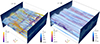 |
Fig. 1. 3D view of the turbulent reconnection structure at t = 4tA and 20tA. The solid lines represent the magnetic field lines colored with the field strength, filled in the 3D current isosurface with |J|≥0.01. This 3D view is based on SD2 listed in Table 1. |
To understand the exchange process of energy in turbulent magnetic reconnection, Figure 2 plots the temporal variation of the magnetic (Figs. 2a and b), kinetic (Fig. 2c), and dissipated (Fig. 2d) energies for all models, where the magnetic energy includes the mean E⟨B⟩ (Fig. 2a) and fluctuation Eb (Fig. 2b) components, and dissipated energy Ediss(t) = E⟨B⟩(t = 0)+Ek(t = 0)−E⟨B⟩(t)−Eb(t)−Ek(t), where the internal energy is defined as  (Γ is the adiabatic index), and its growth is written as ΔEi(t) = Ei(t)−Ei(t = 0). As we can see, all the cases exhibit a similar evolutionary trend, with only differences in temporal progression. The overall evolution process can be divided into three phases: (1) the initial phase of SD reconnection, resulting from instability triggered by the initial velocity perturbation within the current sheet; (2) the fast dissipation and excitation phase, the regular magnetic energy released by reconnection being transferred into kinetic energy, and fluctuation magnetic energy, enhancing the turbulence inside the current sheet to promote the magnetic reconnection process; and (3) the subsequent gradual relaxation phase, showing an approximately dynamic equilibrium between the dissipation of regular magnetic energies and the increase in fluctuations in kinetic and magnetic energies.
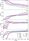 |
Fig. 2. Mean (panel (a)) and fluctuation (panel (b)) magnetic energies, kinetic energy (panel (c)), and dissipated energy (panel (d)) as a function of the evolution time. The solid black line in panel (d) represents the internal energy growth of SD6. |
Taking SD1 as an example, we further clarify the three phases mentioned above: (1) for the first phase before t ∼ 3tA, the regular magnetic energy E⟨B⟩ slowly dissipates and the fluctuation magnetic energy Eb nearly remains unchanged (Figs. 2a and b), while kinetic energy Ek also decreases due to numerical dissipation (Figs. 2c and d), the dissipated energy Ediss, significantly increasing. At this stage, initial velocity perturbation triggers instabilities, leading to the beginning of reconnection and the dissipation of magnetic energy within the current sheet. (2) For the second phase during 3tA ≤ t ≤ 7tA, the energy of the regular magnetic field E⟨B⟩ significantly decreases; the fluctuation magnetic field Eb and kinetic field Ek increase rapidly because of the emergence of turbulence enhancing the reconnection level. (3) For the third phase after t ∼ 7tA, E⟨B⟩ and Eb gradually decrease and increase, respectively, while Ek and Ediss roughly plateau, with the ratio of kinetic energy to dissipated energy being Ek/Ediss ∼ 2% at t = 20tA, showing an approximate relationship of ΔE⟨B⟩ ≃ ΔEk + ΔEb + ΔEdiss.
In addition, we note that the internal energy evolution (ΔEi(t) vs. t) of the adiabatic model SD6 almost coincides with that of the dissipated energy (see SD6 in Fig. 2d), indicating that the dissipated energy is mainly converted into the thermal energy of the gas. This result can help to understand observations in solar flares, as Kontar et al. (2017) pointed out that the magnetic energy released by reconnection is dissipated into gas thermal energy via turbulent interactions, and turbulent kinetic energy accounts for about 1% of the magnetic energy released by reconnection (i.e., dissipated energy).
3.2. Direction-dependent spectral distribution
To investigate the inhomogeneity of reconnection turbulence, we adopted the methodology proposed by Beresnyak (2017) for spectral calculations defined as
 (8)
(8)
where l and kl represent the integration direction (X, Y, and Z) and the wave vector in the plane perpendicular to that direction, respectively, and  denotes the Fourier transform of v or B. Here, we have kl = (ky, kz), (kx, kz), and (kx, ky) for the X, Y, and Z directions, respectively. Based on Eq. (8), we first analyzed the spectral distribution characteristics at the end time (t ∼ 20tA) along three coordinate axis directions.
As shown in Fig. 3, we present the spectral distributions of magnetic (panel (a)) and kinetic (panel (b)) energies in the X, Y, and Z directions. For the spectral distributions of magnetic energy, we can see from Fig. 3a that spectral distributions in the Y direction show a steep slope of E ∝ k−8/3, which indicates the power is more concentrated in the large-scale (small wavenumber) range. In this direction, that is, the X − Z plane parallel to the current sheet, the turbulent magnetic field (small power) within the reconnection region can be well separated from the undisturbed magnetic field (large power) outside the reconnection region. Spectral distributions in the X and Z directions, the Y − Z and X − Y planes perpendicular to the current sheet, show a shallow slope between E ∝ k−8/3 and E ∝ k−5/3 that extends to a large wavenumber (without a significant dissipation process of magnetic energies at small scales). Since both the turbulent magnetic field (within and surrounding the reconnection region) and the undisturbed magnetic field (away from the reconnection region) are included in the same layer when calculating the power spectrum, the small-scale fluctuations of reconnection turbulence within the reconnection region are masked by the surrounding strong, regular, large-scale magnetic fields. Therefore, the power spectra in the X and Z directions do not fully reveal the cascading nature of the reconnection turbulence. The asymmetric phenomenon of spectral distributions reveals the spatial inhomogeneity well of turbulent magnetic field distributions in the reconnection turbulence (see also Zhang et al. 2024 for synthetic synchrotron observations). For the steep spectral feature of the magnetic field, we speculate that the inhomogeneity of the magnetic field and plasma wave instabilities may lead to an anomalous resistivity (e.g., Numata & Yoshida 2002; Silin et al. 2005; Wu et al. 2010), which may indirectly result in the steepening of the power spectrum by affecting the energy cascade processes.
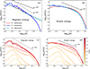 |
Fig. 3. Spectral distributions of magnetic (left column) and velocity (right column) fields. Upper row: Spectral distributions in the three axis directions at t = 20tA. Lower row: Spectral evolutions in the process of turbulence development, where the color bar shows the simulation time in units of Alfvén time tA. These results are based on high-resolution simulations of SD1. |
Spectral distributions of the kinetic energy (see Fig. 3b) exhibit different characteristics from those of the magnetic field. They follow the classical Kolmogorov spectrum of E ∝ k−5/3, except the spectrum in the X direction becomes slightly shallower in the large-scale range, which may be due to the effects of the outflow. This shows that the inhomogeneity of the turbulent flow driven by the reconnection is mainly reflected in the turbulent magnetic field, while the turbulent velocity remains uniform. To effectively reveal the nature of reconnection turbulence, we discuss only the power spectral properties in the Y direction below.
To trace the evolution process of reconnection turbulence, we plotted the time-dependent evolution of spectral distributions of magnetic and kinetic energies in Figs. 3c and d, respectively. With the increase in evolutionary time, the amplitudes of the magnetic and velocity spectra gradually increase to a quasi-saturated state. In the early stages of evolution, the spectra of velocity and the magnetic field only distribute in the large-scale range (about k < 10). Subsequently, the distribution of the spectrum extends to a wider range of wavenumbers. In the late stages, they converge to the scaling of E(k)∝k−8/3 for the magnetic field and E(k)∝k−5/3 for velocity. We note that the spectra t ∼ 20tA (the top red lines) are almost the same as those at t ∼ 15tA (the penultimate red lines), indicating that the turbulence has fully developed. Therefore, our subsequent analysis of the turbulence characteristics focuses on the quasi-steady state at t = 20tA.
3.3. Influence of variable parameters on reconnection turbulence
To evaluate the impact of numerical convergence on our numerical results, we ran the same parameter setting twice (SD1 for 10243 and SD2 for 5123) to compare the spectral distributions. Figure 4 shows the spectral distributions of the magnetic (panel (a)) and kinetic (panel (b)) energies for all cases at t = 20tA. As we can see, spectral distributions of magnetic and kinetic energies display a consistent statistical behavior in the inertial range, with an extended tail at a large wavenumber for SD1. In other words, the simulation for SD1 exhibits a marginally extended inertial range, as it is expected that high-resolution simulations can resolve small-scale structures of reconnection turbulence. This confirms that the resolution of 5123 can capture the spectral feature of the reconnection turbulence cascade. Therefore, to save computing resources, we perform studies of parameter changes in 5123 resolutions below.
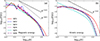 |
Fig. 4. Power spectral distributions of magnetic (panel (a)) and velocity (panel (b)) fields normalized in their mean power at t = 20tA for all models, SD1 to SD6, listed in Table 1. |
We subsequently explore the effect of initial velocity perturbations and explicit resistivity settings on the reconnection turbulence. Due to the lack of differences in spectral distributions between SD2 and SD3, we suggest that the initial velocity perturbation has no significant effect on the reconnection turbulence. Similarly, since SD3 and SD4 exhibit nearly identical spectral distributions, we confirm that explicit resistivity does not significantly influence turbulent reconnection dynamics, which is in agreement with the theoretical predictions of LV99 (e.g., see Kowal et al. 2009, 2017; Beresnyak 2017 for similar results). In addition, we studied the influence of a nonzero guide field on reconnection turbulence (see SD5 of Fig. 4a). For SD5, we see that the magnetic spectrum exhibits an approximate slope of E ∝ k−8/3, with a softening feature in the range of the large wavenumber of k < 10, and the velocity spectrum shows a scaling of E ∝ k−5/3. Consistent with recent 3D MHD simulations (Xiong et al. 2024) and magnetotail observations (Fu et al. 2017; Huang et al. 2023), the existence of the guiding field can promote the transformation of small-scale reconnection points into larger-scale magnetic flux rope structures (Fu et al. 2017; Huang et al. 2023).
As shown in Fig. 5a, we also investigated the influence of the EOS on turbulent reconnection by analyzing the spectral distributions of the magnetic, kinetic, and internal energies. From this figure, we see spectral distributions of magnetic and internal energies of E ∝ k−8/3, and the kinetic energy spectrum E ∝ k−5/3. Remarkably similar spectral distributions from magnetic and internal energies suggest a close connection between magnetic dissipation and gas heating. In addition, a least-squares fitting yields a parabolic relation of p = 0.51B2 − 0.01B + 1 (not shown), which implies that magnetic annihilation during turbulent reconnection enables efficient energy conversion via Joule heating (LV99).
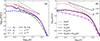 |
Fig. 5. Distributions of magnetic and kinetic energies compared to distributions of internal energies (panel (a)), as well as the solenoidal and compressive components of kinetic energies (panel (b)). Simulations are from the adiabatic state (SD6 listed in Table 1) at t = 20tA. |
3.4. Compressibility of reconnection turbulence
To elucidate the compressibility of reconnection turbulence, we performed a Helmholtz decomposition of the velocity field (v = vsol + vcom) and computed the spectral distributions for two components (Zhdankin et al. 2017), which are defined as  and
and  . Figure 5b shows the spectral distributions of the magnetic field, velocity field, solenoidal, and compressive components. As we can see, although the solenoidal Esol(k) and compressive Ecom(k) components all follow E ∝ k−5/3, the amplitude of the compressive component is much smaller than that of the solenoidal component, with the compressive component Ecom(k) contributing only ∼6.5% to the kinetic energy. Therefore, for the parameter settings of SD6, we suggest that the reconnection turbulence is in a quasi-incompressible state, for which non-reconnection MHD simulations give the proportion of compressible components to be less than 10% (Cho & Lazarian 2003).
3.5. Anisotropy of reconnection turbulence
Figure 6a provides the scale-dependent anisotropy for all models listed in Table 1, with dotted and dashed black lines representing the isotropic and anisotropic scalings, respectively. As can be seen, most of the models exhibit an anisotropic scaling of  at large scales, except SD5 with a nonzero guide field has an isotropic relationship of ℓ∥ ∝ ℓ⊥ throughout the whole spatial region. This indicates that the presence of a guide field affects the spatial anisotropy of the reconnection turbulence. Comparing SD1 to SD2, we found that the anisotropic scaling for SD1 is stronger than that of SD2 at small scales, suggesting that the reconstruction of anisotropic relationships depends on numerical resolution. Since our current simulations have a uniform grid distribution, the geometric constraint of reconnection turbulence poses a challenge to high-precision simulations (see Wang et al. 2025 for the high-resolution simulation of the coronal mass ejection). As we can see in Fig. 1, the reconnection turbulence region occupies only a small portion of the entire space in the direction perpendicular to the current sheet. We expect that simulations of nonuniform meshes may be an effective way to capture the anisotropy of reconnection turbulence, which will be explored in future work.
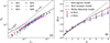 |
Fig. 6. Scale-dependent anisotropy of the velocities for all models (panel (a)) and the intermittency of magnetic and velocity fields (panel (b)). Panel (a): The coordinates ℓ⊥ and ℓ∥ represent the perpendicular and parallel scales of the eddies along the local magnetic field, respectively. Panel (b): The scaling exponent ζ vs. the order of structure functions. Our numerical results, with error bars estimated from the standard deviation, are compared with theoretical predictions from intermittency models: the Kolmogorov, She-Leveque, and Müller-Biskamp. The numerical results that we analyzed, t = 20tA, are based on SD1 listed in Table 1. |
3.6. Intermittency of reconnection turbulence
To investigate the intermittency of reconnection turbulence, we used the extended self-similarity (Benzi et al. 1993) to obtain the scaling exponent (ζ(n)) of the nth-order structure function, which was normalized by the scaling exponent of the third-order structure function. Figure 6b presents the intermittency ofmagnetic and velocity fields for SD1 at t = 20tA. The dotted, dashed, and dot-dashed lines represent the theoretical results from the Kolmogorov (1941,  ), She & Leveque (1994,
 ![Mathematical equation: $ \zeta(n) = \frac{n}{9}+2[1-(\frac{2}{3})^{n/3}] $](/articles/aa/full_html/2025/11/aa53812-25/aa53812-25-eq15.gif) ), and She & Leveque (2000,
), and She & Leveque (2000,  ) models, respectively. As we can see, the velocity and magnetic fields exhibit distinct scaling behaviors. The velocity field scaling at higher orders (n > 3) aligns with the Müller-Biskamp model, corresponding to a 2D sheet-like structure. This finding is consistent with Wang et al. (2025), in which examination of the reconnection core morphology in the current sheet revealed a preference for 2D sheet-like structures. The magnetic field scaling exponents fall between the results of the She-Leveque and Müller-Biskamp models. Compared to the velocity field, this means that the intermittency of the magnetic field is weaker than that of the velocity field.
In the case of lower orders (n = 1 and 2), both velocity and magnetic field scaling exponents slightly exceed the results of all three models. This deviation may arise because classical turbulence theories consider energy cascades from large to small scales. Here, turbulent magnetic reconnection locally concentrates energy release (through the current sheet disruption or magnetic island coalescence). Such an inhomogeneous energy injection could modify the scaling laws (Beresnyak 2019). Furthermore, rapid merging of flux ropes (or magnetic islands in 2D) during reconnection may also enhance the small-scale energy cascade and potentially suppress intermittency (Loureiro et al. 2012).
4. Discussion
In this work, we conducted simulations of SD turbulent reconnection to investigate the properties of reconnection turbulence. Our simulations have incorporated the resistivity effect but have neglected possible viscosity. This is because in magnetic reconnection research, magnetically dominated plasmas are generally considered (e.g., the solar corona and magnetopause; see Lazarian et al. 2020), where resistive dissipation predominantly governs energy conversion within current sheets. This resistive term in the generalized Ohm’s law constitutes the primary mechanism for magnetic diffusion (Priest & Forbes 2000), an assumption supported by extensive observational evidence, including solar flares (Su et al. 2013) and in situ magnetospheric measurements (Burch et al. 2016). Furthermore, energetic transfer in the inertial range is primarily governed by Alfvénic wave interactions (Kraichnan 1965), which are insensitive to dissipation mechanisms (Müller & Grappin 2005).
Our numerical results indicate that explicit resistivity has no significant effect on the properties of reconnection turbulence, at least in the quasi-steady-state phase (see Sect. 3.1), which is consistent with the expectation of LV99 and the results of numerical experiments (e.g., Kowal et al. 2009; Kowal 2012; Kowal et al. 2017). In the early stage of reconnection evolution, resistivity may play a role when the instability of the tearing mode dominates the reconnection process (Huang & Bhattacharjee 2010, 2016). In that case, the influence of different Lundquist numbers should be considered, especially for plasmas above and below the critical Lundquist number (Scrit ∼ 104, see Samtaney et al. 2009). However, once the system transitions to fully developed turbulent reconnection, the effects of resistivity on the reconnection rate can be ignored (Kowal et al. 2009, 2020; Lazarian et al. 2020).
In the case of the guiding field, our results show that the anisotropy of magnetic energy is significantly different from that of other cases. This difference highlights the influence of the guide field on the reconnection turbulence. It is incompatible with the results provided by Kowal et al. (2009), who found that the guide field has no significant impact on the reconnection process. The reason may be that with the high injection rate of turbulence (Pinj ∼ 1.0) in Kowal et al. (2009), the turbulence cascade is strong enough. An appropriate guide field can provide an angle of inclination for the antiparallel magnetic field lines to facilitate the reconnection rate (see Liang et al. 2023 for SD reconnection; and Xu & Lazarian 2022 for a theoretical explanation), resulting in an effective acceleration of particles (Liang et al. 2023; Zhang et al. 2023). This difference requires more numerical simulation work to test.
The reconstruction of scale-dependent anisotropy depends on high-resolution numerical simulations. A deviation in anisotropic relationships at small scales (see Kowal et al. 2017 for similar results) may be caused by numerical dissipation. Therefore, we do indeed need higher-resolution simulations to confirm whether the consistency between the anisotropic scaling of reconnection turbulence and the GS95 theory is robust. We expect that adaptive mesh refinement may be an effective method for achieving high-resolution simulations to capture the anisotropy of reconnection turbulence. We will explore this in future work.
Wang et al. (2025) analyzed the reconnection core within the current sheet, indicating that the reconnection core presents a 2D sheet-like structure, which is consistent with our intermittent result of the velocity field (Fig. 6b). A notable finding is that in reconnection turbulence, the velocity field has a stronger intermittency than the magnetic field; this result contrasts with pure MHD turbulence (e.g., Cho et al. 2003; Haugen et al. 2004; Yoshimatsu et al. 2011; Mallet & Schekochihin 2016). This suggests that the cascade processes of the turbulent magnetic field are constrained by the reconnection processes within the current sheet.
Different from the well-known Kolmogorov spectrum of E ∝ k−5/3, our simulations show an anomalous steep spectrum of the magnetic field of E ∝ k−8/3 along the Y-axis direction, which is a better representation of the spectrum of anisotropic reconnection turbulence. This result is similar to the spectral shape of electron MHD turbulence on kinetic scales in the case of rstrong magnetic fields (Meyrand & Galtier 2013), arising from the strong suppression of the energy cascade along the magnetic field. In the case of reconnection turbulence, reconnection outflows interacting with the magnetic field may result in a negligible parallel (with regard to the local magnetic field) cascade. Therefore, we claim that the anomalous steep spectrum may not be an isolated case across different spatial scales.
5. Summary
Focusing on the properties of reconnection-driven turbulence in SD turbulent magnetic reconnection, we explored the influence of different factors (such as the guide field, resistivity, numerical resolution, and fluid state) on the dynamics and turbulence of reconnection. The main results can be briefly summarized as follows:
-
The evolution of turbulent reconnection can simply be divided into three phases: initial, fast dissipation, and relaxation phases. The dissipation of the antiparallel, regular magnetic fields leads to an increase in turbulent magnetic and kinetic energies.
-
Due to the inhomogeneity of reconnection turbulence, the power spectrum of the turbulent magnetic field presents a direction-dependent spectral distribution, and the power spectrum of turbulent velocity is almost direction-independent.
-
The velocity spectrum shows the expected scaling of E ∝ k−5/3 corresponding to the classic Kolmogorov type, while the slope of the magnetic field spectrum is steeper.
-
Explicit resistivity and the initial velocity disturbance amplitude have no significant effect on the properties of reconnection turbulence, such as spectra and anisotropy, which are consistent with the theoretical prediction of LV99. The presence of a guide field results in an isotropic cascade of reconnection turbulence, which is significantly different from the cascade pattern of pure MHD turbulence.
-
Reconnection turbulence presents a quasi-incompressibility in the adiabatic states, with energy distributions being dominated by the solenoidal component of the velocity. The intermittency of the velocity field is stronger than that of the magnetic field.
Acknowledgments
We thank the anonymous referee for valuable comments that significantly improved the quality of the paper. This work is supported in part by the High-Performance Computing Platform of Xiangtan University. J.F.Z. is grateful for the support from the National Natural Science Foundation of China (No. 12473046), and the Hunan Natural Science Foundation for Distinguished Young Scholars (No. 2023JJ10039). N.Y.Y. is grateful for the support from the National Natural Science Foundation of China (No. 12431014) and the Project of Scientific Research Fund of the Hunan Provincial Science and Technology Department (2024ZL5017). S.M.L. and N.N.G. are grateful for the support from the Xiangtan University Innovation Foundation for Post-graduate Students (Nos. XDCX2024Y164 and XDCX2025Y257).
References
- Benzi, R., Ciliberto, S., Tripiccione, R., et al. 1993, Phys. Rev. E, 48, R29 [CrossRef] [Google Scholar]
- Beresnyak, A. 2017, ApJ, 834, 47 [Google Scholar]
- Beresnyak, A. 2019, Liv. Rev. Comput. Astrophys., 5, 2 [CrossRef] [Google Scholar]
- Biskamp, D. 1996, Ap&SS, 242, 165 [Google Scholar]
- Burch, J. L., Torbert, R. B., & Phan, T. D. 2016, Science, 352, aaf2939 [Google Scholar]
- Carmichael, H. 1964, in NASA Special Publication, ed. W. N. Hess, 50, 451 [NASA ADS] [Google Scholar]
- Chitta, L. P., & Lazarian, A. 2020, ApJ, 890, L2 [Google Scholar]
- Cho, J., & Lazarian, A. 2003, MNRAS, 345, 325 [NASA ADS] [CrossRef] [Google Scholar]
- Cho, J., Lazarian, A., & Vishniac, E. T. 2003, ApJ, 595, 812 [NASA ADS] [CrossRef] [Google Scholar]
- Dere, K. P. 1996, ApJ, 472, 864 [Google Scholar]
- Dong, C., Wang, L., Huang, Y.-M., et al. 2022, Science Adv., 8, eabn7627 [Google Scholar]
- Drake, J. F., Swisdak, M., Che, H., & Shay, M. A. 2006, Nature, 443, 553 [Google Scholar]
- Eriksson, S., Elkington, S. R., Phan, T. D., et al. 2004, J. Geophys. Res., 109, A12203 [Google Scholar]
- Eyink, G. L., Lazarian, A., & Vishniac, E. T. 2011, ApJ, 743, 51 [Google Scholar]
- Fu, H. S., Vaivads, A., Khotyaintsev, Y. V., et al. 2017, Geophys. Res. Lett., 44, 37 [Google Scholar]
- Gehrels, N., Ramirez-Ruiz, E., & Fox, D. B. 2009, ARA&A, 47, 567 [NASA ADS] [CrossRef] [Google Scholar]
- Goldreich, P., & Sridhar, S. 1995, ApJ, 438, 763 [Google Scholar]
- Harris, E. G. 1962, Il Nuovo Cimento, 23, 115 [Google Scholar]
- Haugen, N. E. L., Brandenburg, A., & Dobler, W. 2004, Phys. Rev. E, 70, 016308 [NASA ADS] [CrossRef] [Google Scholar]
- Hirayama, T. 1974, Sol. Phys., 34, 323 [Google Scholar]
- Huang, Y.-M., & Bhattacharjee, A. 2010, Phys. Plasmas, 17, 062104 [Google Scholar]
- Huang, Y.-M., & Bhattacharjee, A. 2016, ApJ, 818, 20 [NASA ADS] [CrossRef] [Google Scholar]
- Huang, S. Y., Zhang, J., Xiong, Q. Y., et al. 2023, ApJ, 958, 189 [Google Scholar]
- Kolmogorov, A. 1941, Akademiia Nauk SSSR Doklady, 30, 301 [Google Scholar]
- Kontar, E. P., Perez, J. E., Harra, L. K., et al. 2017, Phys. Rev. Lett., 118, 155101 [NASA ADS] [CrossRef] [Google Scholar]
- Kopp, R. A., & Pneuman, G. W. 1976, Sol. Phys., 50, 85 [Google Scholar]
- Kowal, G., & de Gouveia Dal Pino, E. M., & Lazarian, A., 2012, Phys. Rev. Lett., 108, 241102 [NASA ADS] [CrossRef] [Google Scholar]
- Kowal, G., Lazarian, A., Vishniac, E. T., & Otmianowska-Mazur, K. 2009, ApJ, 700, 63 [Google Scholar]
- Kowal, G., Falceta-Gonçalves, D. A., Lazarian, A., & Vishniac, E. T. 2017, ApJ, 838, 91 [NASA ADS] [CrossRef] [Google Scholar]
- Kowal, G., Falceta-Gonçalves, D. A., Lazarian, A., & Vishniac, E. T. 2020, ApJ, 892, 50 [Google Scholar]
- Kraichnan, R. H. 1965, Phys. Fluids, 8, 1385 [Google Scholar]
- Kulpa-Dybeł, K., Kowal, G., Otmianowska-Mazur, K., Lazarian, A., & Vishniac, E. 2010, A&A, 514, A26 [NASA ADS] [CrossRef] [EDP Sciences] [Google Scholar]
- Lazarian, A., & Vishniac, E. T. 1999, ApJ, 517, 700 [Google Scholar]
- Lazarian, A., & Vishniac, E. T. 2009, Rev. Mex. Astron. Astrofis. Conf. Ser., 36, 81 [Google Scholar]
- Lazarian, A., Eyink, G. L., Jafari, A., et al. 2020, Phys. Plasmas, 27, 012305 [NASA ADS] [CrossRef] [Google Scholar]
- Li, L., Song, H., Peter, H., et al. 2024, ApJ, 967, 130 [Google Scholar]
- Liang, S.-M., Zhang, J.-F., Gao, N.-N., & Xiao, H.-P. 2023, ApJ, 952, 93 [Google Scholar]
- Lin, J., & Forbes, T. G. 2000, J. Geophys. Res., 105, 2375 [Google Scholar]
- Loureiro, N. F., Uzdensky, D. A., Schekochihin, A. A., Cowley, S. C., & Yousef, T. A. 2009, MNRAS, 399, L146 [Google Scholar]
- Loureiro, N. F., Samtaney, R., Schekochihin, A. A., & Uzdensky, D. A. 2012, Phys. Plasmas, 19, 042303 [NASA ADS] [CrossRef] [Google Scholar]
- Mallet, A., & Schekochihin, A. A. 2016, MNRAS, 466, 3918 [Google Scholar]
- Meyer, M., Horns, D., & Zechlin, H. S. 2010, A&A, 523, A2 [NASA ADS] [CrossRef] [EDP Sciences] [Google Scholar]
- Meyrand, R., & Galtier, S. 2013, Phys. Rev. Lett., 111, 264501 [NASA ADS] [CrossRef] [Google Scholar]
- Mignone, A., Bodo, G., Vaidya, B., & Mattia, G. 2018, ApJ, 859, 13 [CrossRef] [Google Scholar]
- Müller, W.-C., & Biskamp, D. 2000, Phys. Rev. Lett., 84, 475 [CrossRef] [Google Scholar]
- Müller, W.-C., & Grappin, R. 2005, Phys. Rev. Lett., 95, 114502 [Google Scholar]
- Numata, R., & Yoshida, Z. 2002, Phys. Rev. Lett., 88, 045003 [Google Scholar]
- Oishi, J. S., Mac Low, M.-M., Collins, D. C., & Tamura, M. 2015, ApJ, 806, L12 [NASA ADS] [CrossRef] [Google Scholar]
- Parker, E. N. 1957, J. Geophys. Res., 62, 509 [Google Scholar]
- Petschek, H. E. 1964, NASA Spec. Pub., 50, 425 [NASA ADS] [Google Scholar]
- Priest, E., & Forbes, T. 2000, Magnetic Reconnection: MHD Theory and Applications (Cambridge, UK: Cambridge University Press) [Google Scholar]
- Puzzoni, E., Mignone, A., & Bodo, G. 2021, MNRAS, 508, 2771 [CrossRef] [Google Scholar]
- Samtaney, R., Loureiro, N. F., Uzdensky, D. A., Schekochihin, A. A., & Cowley, S. C. 2009, Phys. Rev. Lett., 103, 105004 [NASA ADS] [CrossRef] [Google Scholar]
- She, Z.-S., & Leveque, E. 1994, Phys. Rev. Lett., 72, 336 [Google Scholar]
- Shibata, K., Masuda, S., Shimojo, M., et al. 1995, ApJ, 451, L83 [Google Scholar]
- Silin, I., Büchner, J., & Vaivads, A. 2005, Phys. Plasmas, 12, 062902 [Google Scholar]
- Sturrock, P. A. 1966, Nature, 211, 695 [Google Scholar]
- Su, Y., Veronig, A. M., Holman, G. D., et al. 2013, Nat. Phys., 9, 489 [Google Scholar]
- Sweet, P. A. 1958, The Observatory, 78, 30 [Google Scholar]
- Tavani, M., Bulgarelli, A., Vittorini, V., et al. 2011, Science, 331, 736 [CrossRef] [PubMed] [Google Scholar]
- Uzdensky, D. A., Loureiro, N. F., & Schekochihin, A. A. 2010, Phys. Rev. Lett., 105, 235002 [Google Scholar]
- Vishniac, E. T., Pillsworth, S., Eyink, G., et al. 2012, Nonlinear Processes Geophys., 19, 605 [Google Scholar]
- Wang, Y., Cheng, X., Ding, M., et al. 2023, ApJ, 954, L36 [NASA ADS] [CrossRef] [Google Scholar]
- Wang, Y., Cheng, X., & Ding, M. 2025, ApJ, 985, 43 [Google Scholar]
- Wu, G., Huang, G., & Ji, H. 2010, ApJ, 720, 771 [Google Scholar]
- Xiong, Q. Y., Huang, S. Y., Zhang, J., et al. 2024, Geophys. Res. Lett., 51, e2024GL109356 [Google Scholar]
- Xu, S., & Lazarian, A. 2022, ApJ, 942, 21 [Google Scholar]
- Yoshimatsu, K., Schneider, K., Okamoto, N., Kawahara, Y., & Farge, M. 2011, Phys. Plasmas, 18, 092304 [Google Scholar]
- Zhang, J.-F., Xu, S., Lazarian, A., & Kowal, G. 2023, J. High Energy Astrophys., 40, 1 [Google Scholar]
- Zhang, J.-F., Liang, S.-M., & Xiao, H.-P. 2024, ApJ, 969, 139 [Google Scholar]
- Zhdankin, V., Werner, G. R., Uzdensky, D. A., & Begelman, M. C. 2017, Phys. Rev. Lett., 118, 055103 [NASA ADS] [CrossRef] [Google Scholar]
All Tables
All Figures
|
Fig. 1. 3D view of the turbulent reconnection structure at t = 4tA and 20tA. The solid lines represent the magnetic field lines colored with the field strength, filled in the 3D current isosurface with |J|≥0.01. This 3D view is based on SD2 listed in Table 1. |
| In the text | |
|
Fig. 2. Mean (panel (a)) and fluctuation (panel (b)) magnetic energies, kinetic energy (panel (c)), and dissipated energy (panel (d)) as a function of the evolution time. The solid black line in panel (d) represents the internal energy growth of SD6. |
| In the text | |
|
Fig. 3. Spectral distributions of magnetic (left column) and velocity (right column) fields. Upper row: Spectral distributions in the three axis directions at t = 20tA. Lower row: Spectral evolutions in the process of turbulence development, where the color bar shows the simulation time in units of Alfvén time tA. These results are based on high-resolution simulations of SD1. |
| In the text | |
|
Fig. 4. Power spectral distributions of magnetic (panel (a)) and velocity (panel (b)) fields normalized in their mean power at t = 20tA for all models, SD1 to SD6, listed in Table 1. |
| In the text | |
|
Fig. 5. Distributions of magnetic and kinetic energies compared to distributions of internal energies (panel (a)), as well as the solenoidal and compressive components of kinetic energies (panel (b)). Simulations are from the adiabatic state (SD6 listed in Table 1) at t = 20tA. |
| In the text | |
|
Fig. 6. Scale-dependent anisotropy of the velocities for all models (panel (a)) and the intermittency of magnetic and velocity fields (panel (b)). Panel (a): The coordinates ℓ⊥ and ℓ∥ represent the perpendicular and parallel scales of the eddies along the local magnetic field, respectively. Panel (b): The scaling exponent ζ vs. the order of structure functions. Our numerical results, with error bars estimated from the standard deviation, are compared with theoretical predictions from intermittency models: the Kolmogorov, She-Leveque, and Müller-Biskamp. The numerical results that we analyzed, t = 20tA, are based on SD1 listed in Table 1. |
| In the text | |
Current usage metrics show cumulative count of Article Views (full-text article views including HTML views, PDF and ePub downloads, according to the available data) and Abstracts Views on Vision4Press platform.
Data correspond to usage on the plateform after 2015. The current usage metrics is available 48-96 hours after online publication and is updated daily on week days.
Initial download of the metrics may take a while.