| Issue |
A&A
Volume 703, November 2025
|
|
|---|---|---|
| Article Number | A64 | |
| Number of page(s) | 18 | |
| Section | Stellar structure and evolution | |
| DOI | https://doi.org/10.1051/0004-6361/202553922 | |
| Published online | 07 November 2025 | |
SN 2022xlp: The second-known well-observed, intermediate-luminosity Iax supernova
1
Department of Experimental Physics, Institute of Physics, University of Szeged, Dóm tér 9, 6720 Szeged, Hungary
2
Baja Astronomical Observatory of the University of Szeged, Szegedi út, Kt. 766, 6500 Baja, Hungary
3
HUN-REN CSFK Konkoly Observatory, Konkoly Thege M. út 15-17, Budapest 1121, Hungary
4
HUN-REN-SZTE Stellar Astrophysics Research Group, Szegedi út, Kt. 766, 6500 Baja, Hungary
5
Department of Astronomy, University of Texas at Austin, 2515 Speedway, Stop C1400, Austin, TX 78712-1205, USA
6
Steward Observatory, University of Arizona, 933 North Cherry Avenue, Tucson, AZ 85721-0065, USA
7
Department of Astronomy and Astrophysics, University of California, Santa Cruz, CA 95064, USA
8
Institute of Space Sciences (ICE, CSIC), Campus UAB, Carrer de Can Magrans, s/n, E-08193 Barcelona, Spain
9
Institut d’Estudis Espacials de Catalunya (IEEC), E-08034 Barcelona, Spain
10
Department of Physics and Astronomy, Rutgers, the State University of New Jersey, 136 Frelinghuysen Road, Piscataway, NJ 08854-8019, USA
11
Las Cumbres Observatory, 6740 Cortona Drive, Suite 102, Goleta, CA 93117-5575, USA
12
Department of Physics, University of California, Santa Barbara, CA 93106-9530, USA
13
Center for Interdisciplinary Exploration and Research in Astrophysics (CIERA), and Department of Physics and Astronomy, Northwestern University, Evanston, IL 60208, USA
14
ELTE Eötvös Loránd University, Institute of Physics and Astronomy, Pázmány Péter sétány 1A, Budapest 1117, Hungary
15
National Astronomical Research Institute of Thailand (NARIT), Chiang Mai 50180, Thailand
⋆ Corresponding author: This email address is being protected from spambots. You need JavaScript enabled to view it.
Received:
27
January
2025
Accepted:
18
July
2025
Abstract
Context. We present a detailed multicolor photometric and spectroscopic analysis of type Iax supernova SN 2022xlp. With a V-band absolute magnitude light curve peaking at Mmax(V) = − 16.04 ± 0.25 mag, this object is regarded as the second determined well-observed Iax supernova in the intermediate luminosity range after SN 2019muj.
Aims. Our research aims to explore the question of whether the physical properties vary continuously across the entire luminosity range. We also investigate the chemical abundance profiles and the characteristic physical quantities of the ejecta, followed by tests of the predictions of hydro simulations.
Methods. The pseudo-bolometric light curve was calculated using optical (BgVriz) and UV (Swift UVOT UVW2,UVM2, UVW1,U,B) light curves and fits with a radiation diffusion Arnett model to constrain the average optical opacity, ejected mass, and initial nickel mass produced in the explosion. We analyzed the color evolution of SN 2022xlp and compared it with that of other Iax supernovae with different peak luminosities. We used the spectral tomography method to determine the radial profiles of physical properties and abundances of the ejecta, comparing them with a set of hydrodynamic pure deflagration models.
Results. SN 2022xlp shows a relatively rapid color evolution due to the decreasing photospheric temperature in the early phase. The estimated bolometric flux peaks at 8.87 × 1041 erg s−1 and indicates the production of radioactive nickel as M(56Ni) = 0.0215 ± 0.009 M⊙. According to the best-fit model, the explosion energy is (2.066 ± 0.236)×1049 erg and the ejecta mass is 0.142 ± 0.015 M⊙. The performed spectral tomography analysis shows that the determined physical quantities agree well with the predictions of the deflagration simulations, with modifications regarding the increased Na abundance and the more massive outer layers. SN 2022xlp bridges the previously existing luminosity gap, together with SN 2019muj, and supports the assumption of continuous variation in the physical properties across the SN Iax subclass.
Key words: radiative transfer / techniques: photometric / techniques: spectroscopic / supernovae: general / supernovae: individual: SN 2022xlp
© The Authors 2025
 Open Access article, published by EDP Sciences, under the terms of the Creative Commons Attribution License (https://creativecommons.org/licenses/by/4.0), which permits unrestricted use, distribution, and reproduction in any medium, provided the original work is properly cited.
This article is published in open access under the Subscribe to Open model. This email address is being protected from spambots. You need JavaScript enabled to view it. to support open access publication.
1. Introduction
It is widely accepted that thermonuclear supernovae (SNe) are fusion explosions of white dwarfs (WDs) in special binary systems. While modern observations and theoretical studies, such as radiative energy transfer modeling in SN ejecta and hydrodynamic simulations of explosions, have allowed us to unveil the nature and properties of thermonuclear SNe, some key questions remain unresolved. Over the past few decades, transient survey programs have discovered several subtypes of thermonuclear events besides the Branch-normal SNe Ia Branch et al. (2006). Currently, one of the most important questions pertains to exactly how the fusion explosion of a WD occurs and what the progenitor systems are for the different types of thermonuclear SNe. In this study, we present a detailed multicolor photometric and spectroscopic analysis of a special thermonuclear supernova, SN 2022xlp, which belongs to the Iax subclass.
The spectra of SNe Iax (often referred to as 2002cx-like objects after the first known SN of this type of these peculiar transients (Li et al. 2003) are similar to those of normal SNe Ia in terms of line-forming ions. SNe Iax always have lower peak luminosity, lower photospheric velocities, shorter rise times, and kinetic energies. Furthermore, these observables present a strong diversity in the subclass. SN 2019gsc, one of the least luminous SN Iax, had a peak brightness of Mmax(V) = − 13.99 mag in the V-band (Srivastav et al. 2020); whereas SN 2011ay reached a peak at Mmax(V) = − 18.39 mag (Szalai et al. 2015). The rise time of SNe Iax typically falls between 10 and 15 days (see, e.g., Foley et al. 2009, Srivastav et al. 2020, and Singh et al. 2024), while the decay phase of their light curves (LCs) is faster than that of the normal SNe Ia. In the case of SNe Iax, the value of the parameter Δm15 (the decrease in brightness within the first 15 days following the peak) typically falls between ∼0.6 − 1.3 mag. Finally, both the photospheric velocity and the mass of the produced 56Ni isotopes display a broad diversity; for instance, vphot = 2500 km/s and M56Ni = 0.003 M⊙ were found in the case of SN 2008ha (Foley et al. 2009), while the corresponding values for SN 2011ay, for instance, are vphot = 9300 km/s and M56Ni = 0.225 M⊙ (Szalai et al. 2015).
The spectral features of SNe Iax and normal SNe Ia also display significant differences in their evolution. In SNe Iax, (i) the lines of the intermediate mass elements (IMEs) are weaker than those of the iron group elements (IGEs); (ii) the absorption components of the P Cygni line profiles cover shorter range of wavelength, indicating that the line-forming processes of the particular ions take part in a narrow atmospheric shell (caused by either the steeper density or temperature gradient). At later epochs, SNe Iax never enter the pure nebular phase; while some dominant forbidden emission lines are present, the late-time spectra show continuum flux and permitted P Cygni profiles (e.g. Fe II, Na I D, Ca II) even at more than ∼100 days after explosion (Foley et al. 2016a). These properties possibly indicate that a bound remnant is left over after the unsuccessful disruption of a WD, which is assumed to produce outflow by the super-Eddington wind process (Foley et al. 2016b).
The most successful hydrodynamic simulations, for instance, reported in the studies of Fink et al. (2014), Lach et al. (2022), Kromer et al. (2015), and Long et al. (2014) have also shown that the pure deflagration explosion of a WD is sufficient to explain the diversity of the observed properties of SNe Iax. The strength of the initial deflagration determines the kinetic energy and, thus, the expansion velocity of the ejecta. In contrast to the detonation processes, the kinetic energy produced during pure deflagration is too low to disrupt the whole WD. Thus, less material is ejected, producing a lower-density profile compared to normal SNe Ia. The models predict that the abundance profile of an SN Iax is almost constant and that IGEs have higher abundances than in normal SNe Ia. According to these simulations, the most abundant elements and isotopes are 56Ni, O, and C.
In the case of typical SNe Ia, a relation exists between the peak absolute brightness and the Δm15 parameter (usually called the Phillips relation, Pskovskii 1977; Phillips 1993), which allows for the use of SNe Ia as precise distance indicators. Although SNe Iax basically do not follow this relation (Jha 2017), the question arises of whether there are similar correlations regarding some of their physical parameters. Previously, there have been attempts to find such pairs of correlated parameters, such as the absolute magnitude of the peak in the V band and the photospheric velocity, or the Δm15(V) parameter and the photospheric velocity (McClelland et al. 2010; Tomasella et al. 2016). These studies, however, could not unambiguously determine the existence of such correlations due to the limited sample size and the existence of outliers, such as SNe 2009ku (Narayan et al. 2011), or 2014ck (Tomasella et al. 2016).
SN 2022xlp is considered special even within the Iax subclass because it is only the second well-observed in the intermediate-luminosity range (after SN 2019muj, Barna et al. 2021). We present the context of the discovery of SN 2022xlp, along with the main properties of the host galaxy NGC 3938 in Section 2. The observations, data reduction procedures, and steps for detailed photometric and spectroscopic analysis are presented in Sections 3, 4, and 5, respectively. We summarize the results and conclusions of our study in Section 6.
2. SN 2022xlp and its host galaxy NGC 3938
SN 2022xlp was discovered by Koichi Itagaki on T0 = 59865.808 MJD with ∼17 mag in apparent magnitude (Itagaki 2022). The supernova exploded in the NGC 3938 galaxy at RA = 11:52:49.560, Dec = +44:06:03.60 (J2000). The redshift and the distance modulus of the host galaxy are adopted from the NASA Extragalactic Database (NED1) and are listed in Table 1. The distance of NGC 3938 was measured with the expanding photosphere method (EPM) based on the data analysis of Type IIP SN 2005ay (which appeared earlier in this galaxy); the result in the I-band is dI = 21.9 Mpc, while in the V-band dV = 22.4 Mpc (Rodríguez et al. 2014). For further analysis, we used the average of these values d = 22.15 Mpc as the distance from the host galaxy. The galactic extinction data in the direction of NGC 3938 were adopted from NED and listed in Table 1. The galactic color excess is E(B − V) = 0.019 mag. SN 2022xlp was classified as SN Iax by Kenta Taguchi, Keiichi Maeda, and Miho Kawabata (Kyoto University) based on the first spectrum obtained at 59867.8 MJD (Taguchi et al. 2022). The image of NGC 3938 with SN 2022xlp can be seen in Fig. 1, while the detailed data of these objects are listed in Table 1.
Data pertaining to NGC 3938 and SN 2022xlp.
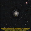 |
Fig. 1. Image of NGC 3938 hosted the SN 2022xlp. This picture was taken with the BRC80 telescope in the Baja Astronomical Observatory of the University of Szeged. |
3. Observations and data processing
3.1. Photometry
The long-term multicolor photometric follow-up of the supernova was started at the Baja Astronomical Observatory of the University of Szeged with the BRC80 telescope right after the classification, during the rising phase. The instrument is a 0.8m Ritchey-Chrétien-Nasmyth (RCN) telescope, with a focal length of 5700 mm and an f/7 light-gathering power. The telescope is equipped with Johnson-Cousins-Bessel BV and Sloan ugriz filters mounted in front of an FLI PL230-42 CCD camera, which has a 2048 × 2048 sensitive back-illuminated E2V CCD chip. The image scale is 0.55 arcsec/px, totaling to a field of view of 18.86 × 18.86′. We carried out standard multicolor photometric observations in 17 nights between −5 and 150 days relative to the V-band maximum. The exposure times are listed in the Table A.1. The instrumental magnitudes of the SN were calculated using the image subtraction method and transformed into the standard photometric system (for further technical details, see Appendix A).
After maximum light, ground-based photometric follow-up was also obtained with the 1m telescopes of the Las Cumbres Observatory (LCO2) network located at the Teide Observatory (Tenerife, Canary Islands, Spain) and McDonald Observatory (Fort Davis, Texas, USA) via the Global Supernova Project (GSP) in the SDSS gri and Johnson-Cousins-Bessel BV bands. The data obtained by the BRC80 telescope were reduced by our IRAF-based reduction and photometric software, while the median combination and the aperture photometry of LCO data were performed by applying self-written pipelines using the FITSH software Pál (2012). The long-term multicolor standard photometric magnitudes of the SN 2022xlp are listed in Table B.1, while the standard multicolor photometric LCs are plotted in Fig. 2. For the epoch with no available measurements in the Johnson-Cousins-Bessel B and V bands at LCO, these magnitudes were calculated by transformation of SDSS band magnitudes according to Tonry et al. (2012), while data points with errors greater than ∼0.1 mag were rejected.
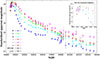 |
Fig. 2. Ground-based photomety of SN 2022xlp. The zoom-inset highlights the near-maximum observations. Data measured by the BRC80 telescope are marked with triangles, while filled circles mark the LCO data points. |
In addition to ground-based photometry, the Neil Gehrels Swift Observatory Ultraviolet/Optical Telescope (UVOT, hereafter Swift; Burrows et al. 2005; Roming et al. 2005; Gehrels et al. 2004) measured the brightness in the UV-band filters (W2, M2, W1, U, B) at three epochs between –4 and 3 days relative to the V-band maximum. The Swift data were downloaded from the Swift archive. These data were reduced using standard HEAsoft tasks. Individual frames were summarized with the uvotimsum task. The magnitudes were determined via aperture photometry using the task uvotsource and adopting the most recent zero-points from the caldb database. The UV photometric dataset is presented in Table C.1.
3.2. Spectroscopy
The first spectrum was taken with the KOOLS-IFU spectrograph attached to the 3.8-m Seimei telescope at the Okayama Observatory. After the classification, a spectroscopic follow-up was obtained with the 3m Shane telescope located in the Lick Observatory of the University of California. The spectra were observed with the Shane telescope’s Kast Dual Channel Spectrograph (Miller & Stone 1993). The telescope’s three-meter primary mirror and the spectrograph’s efficient light throughput enabled the recording of spectra with a high signal-to-noise ratio (S/N), required by spectral tomography. To reduce the Kast data, we used the UCSC Spectral Pipeline3 (Siebert et al. 2020) data reduction pipeline based on procedures outlined by Foley et al. (2003), Silverman et al. (2012), and references therein. The two-dimensional (2D) spectra were bias-corrected, flat-field corrected, adjusted for varying gains across different chips and amplifiers, and trimmed. The one-dimensional (1D) spectra were extracted using the optimal algorithm (Horne 1986). The spectra were wavelength-calibrated using internal comparison-lamp spectra with linear shifts applied by cross-correlating the observed night-sky lines in each spectrum to a master night-sky spectrum. Flux calibration and telluric correction were performed using standard stars at an air mass similar to that of the science exposures. We combined the sides by scaling one spectrum to match the flux of the other in the overlap region and using their error spectra to correctly weight the spectra when combining. More details of this process are discussed in prior works (Foley et al. 2003; Silverman et al. 2012; Siebert et al. 2020). These observations were primarily coordinated using YSE-PZ (Coulter et al. 2022, 2023), an open source, general-purpose target and observation management (TOM) platform.
Main photometric parameters of the multicolor LCs of SN 2022xlp.
From +23 days since the V-band maximum, the 2m Faulkes Telescope North of the Las Cumbres Observatory (LCO4) also joined the spectral follow-up through the Global Supernova Project. Spectra were taken with the FLOYDS spectrograph5. The 1D spectra were extracted using the FLOYDS pipeline6.
In the case of the classification spectrum and the spectra taken by the 2m Faulkes telescope, we applied a moving-averaging process to improve the S/N. We performed a wavelength-dependent spectral flux calibration on all spectra according to match the multicolor photometry. The dataset was corrected for extinction, reddening, and redshift with values adopted from the NED database (see Table 1). In the absence of a high-resolution spectrum, it was not possible to precisely measure the extinction of the host galaxy using the Na I D lines. Since the explosion occurred in a region of the NGC 3938 disk with less interstellar matter, viewed face-on, we neglected the local extinction and only applied a correction for the Galactic component. The series of normalized spectra can be seen in Fig. 3, where the main spectral features are also highlighted. The log of spectral observations is summarized in Table D.1.
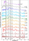 |
Fig. 3. Optical spectra of SN 2022xlp. The characteristic spectral features are highlighted by gray stripes. The phase relative to the V-band maximum (tV) and the time since the explosion (texp) are also marked. |
4. Photometry and light curve analysis
We fit individual LCs with simple polynomial functions to determine the characteristic parameters, namely the MJD of the peak brightness, Δm15, and the apparent and absolute magnitudes of the peak. Hereafter, we use the moment of the V-band maximum as a reference time, since most of the data points are available in this filter. The determined LC parameters are listed in Table 2. According to the peak absolute brightnesses of the Mpeak(V) = − 16.04 ± 0.25 mag and Mpeak(g) = − 16.05 ± 0.25 mag, SN 2022xlp is the second intermediate luminous supernova studied in detail along with SN 2019muj (Mpeak(V) = − 16.42 ± 0.06 mag and Mpeak(g) = − 16.48 ± 0.07 mag) (Barna et al. 2021). The obtained decline rates are  and
and  indicating a slower dimming than that of SN 2019muj (Δm15(V) = 1.2 mag and Δm15(g) = 2.0 mag Barna et al. 2021).
The color evolution of SN 2022xlp can be seen in Fig. 5, along with a comparison to other Iax supernovae. We applied extinction corrections to the color indexes with the formula (mλ1 − mλ2)real = (mλ1 − mλ2)obs − (Rλ1 − Rλ2)×E(B − V), where (mλ1 − mλ2)real is the extinction-corrected color index, while (mλ1 − mλ2)obs is the observed color index, E(B − V) is the color excess, and Rλ is a filter-dependent coefficient. The time dependence of the various color indices shows a very strong similarity in the case of SN 2022xlp and SN 2019muj. According to the B–V, g–r, and g–i color changes, a relatively steep reddening occurs in the very early phase between about −5 and 18 days and the V-band maximum. The B-V color index changes ∼1.3 mag in ∼23 days, while the g-r and g-i color indexes vary ∼1.0 mag and ∼1.2 mag, respectively. This reddening is much faster compared to normal SNe Ia (Milne et al. 2010). The r–i color shows a monotonic increase, which becomes quasi-linear after 16 days following the V maximum. In Fig. 5, the color evolution of SN 2022xlp is compared to a fainter and brighter SNe Iax, SN 2008ha and SN 2012Z. All SNe Iax show an overall similar color evolution with minor differences in the amplitude and steepness of the initial reddening. The fainter SNe Iax shows a faster color change rate. The amplitude of the color change is greater in the case of brighter Iax supernovae. After the reddening maximum, the color indices start to decline slowly andquasi-linearly.
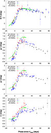 |
Fig. 5. Evolution of different color indexes compared to another SNe Iax (SN 2019muj – (Barna et al. 2021), SN 2012Z – (Stritzinger et al. 2015), and SN 2008ha – (Foley et al. 2009; Stritzinger et al. 2014)). SN 2022xlp shows a very similar color evolution to SN 2019muj. The color indexes are corrected for the extinction as described in Sect. 4. We adopted the color excess from the papers listed above. |
A pseudo-bolometric LC is created by the integration of spectral flux densities calculated from the multicolor magnitudes. The optical flux is calculated with the SuperBol Python software (Nicholl 2018). We calculate the UV flux with the Swift UVOT magnitudes. At every third epoch, the magnitudes were corrected to extinction, converted to spectral flux densities, and integrated up to the effective wavelength of the B filter. According to these three epochs, the time evolution of the UV flux follows a linear decay trend. We fit the FUV − tV data points with a linear function to calculate the UV part of the total flux for other epochs when only optical data areavailable.
The IR contribution was estimated from the i band flux. We adopted FIR = λFλ/3 according to the integrated formula of the Rayleigh-Jeans assumption, where λ is the effective wavelength of the i filter.
We performed an analysis of the pseudo-bolometric LC via the fitting of the theoretical (Arnett) model. The expansion of the supernova ejecta was assumed to be spherically symmetric and homologous (Magee et al. 2016). At the pre-maximum epochs, the ejecta can be modeled as an optically thick expanding fireball model. The energy released by the decay of 56Ni (with half-life time t1/2 = 6.077 days and the energy production rate ϵ56Ni = 3.9 × 10¹⁰ erg/s/g) is in agreement with the decreasing internal energy caused by the adiabatic expansion and radiation. Thus, the temperature can remain nearly constant and the luminosity of the supernova has a quadratic dependence on time, expressed as
 (1)
(1)
where R is the radius of the supernova photosphere, Tph and vph are its temperature and expansion velocity, and texp is the time since the explosion. At maximum light, the emitted energy is equal to the energy released by the decay of 56Ni; thus, the peak luminosity depends on the nickel mass produced. The post-maximum phase of the LC is also influenced by the decay of 56Ni and its daughter isotope 56Co, and the decline rate is proportional to the effective diffusion time of the photons:  , where td is the diffusion time, κ is the opacity, M is the mass of the supernova ejecta, and Ek is its kinetic energy. The opacity is mainly affected by the Thomson-scattering of photons on free electrons and the fluorescenceof IGEs.
The time-dependent bolometric flux can be expressed with a semi-analytic model as presented in Chatzopoulos et al. (2012), which is based on the radioactive decay and photodiffusion model described in Arnett (1982) and Valenti et al. (2008) as
![Mathematical equation: $$ \begin{aligned}&L(t) = M_{^{56}Ni}\exp {(-x^2)}\left[1-\exp {\left(-\frac{t_{\gamma }}{t_{\rm exp}^2} \right)}\right] \times \nonumber \\&\times \left[(\epsilon _{^{56}Ni}-\epsilon _{^{56}Co})\int _{0}^x 2z\exp {(z^2-2z{ y})}\mathrm{d}z + \right. \nonumber \\&+ \left. \epsilon _{^{56}Co}\int _{0}^x 2z\exp {(z^2-2z{ y}+2zs)}\mathrm{d}z \right], \end{aligned} $$](/articles/aa/full_html/2025/11/aa53922-25/aa53922-25-eq27.gif) (2)
(2)
where texp is the time since the explosion, M56Ni is the mass of the 56Ni produced by the explosion, and ϵ56Ni and ϵ56Co are the energy production rates of the 56Ni and 56Co isotopes, respectively. The factor tγ = (3κγMej)/(4πv2) accounts for the gamma leakage, where kγ is the gamma ray opacity, v is the expansion velocity, Mej is the mass of the ejecta. The remaining parameters are defined by the following expressions: x = t/td, y = td/(2tNi), z = 1/(2td), and s = td(tCo − tNi)/(2tCotNi), where  is the effective diffusion time, κ is the total opacity and β = 13.8 is a fixed LC parameter, which is related to the density distribution (Arnett 1982). The synthetic LC produced by the presented semi-analytic model is fit to the pseudo-bolometric LC by the MINIM code (Chatzopoulos et al. 2013). The best-fit model parameters are listed in Table 3, while the pseudo-bolometric LC and the best-fit synthetic model are shown in Fig. 4. According to the determined Arnett model parameters, the total mass of the ejecta and the explosion energy can be calculated with the following formulae:
 (3)
(3)
 (4)
(4)
Best-fit Arnett model parameters and the calculated ejecta properties.
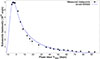 |
Fig. 4. Pseudo-bolometric LC of SN 2022xlp and the best-fit synthetic light model. |
where vph is the photospheric velocity, κγ = 0.025 cm2g−1 according to (Guttman et al. 2024). In the case of Eq. (4), constant density ejecta is assumed. The photospheric velocity can be determined by spectral analysis, which is described in Sect. 5. We can determine the mass and kinetic energy of the ejecta based on the effective diffusion time with the formulae adopted from Ganeshalingam et al. (2012):
 (5)
(5)
 (6)
(6)
Regarding the determined model parameters, the mass of 56Ni is comparable and slightly lower than in the case of SN 2019muj, as predicted by similar absolute peak brightnesses. The nickel mass determined from the Arnett model fit is M56Ni = 0.0191 ± 0.0025 M⊙, while in the case of SN 2019muj, it is M56Ni = 0.031 ± 0.005 M⊙ (Barna et al. 2021). The effective diffusion time is similar for SN 2019muj and SN 2022xlp, 7.1 ± 0.5 days for SN 2019muj and 6.46 ± 1.73 days for SN 2022xlp, while the gamma leakage timescale differs significantly, with 5.5 ± 1.5 days for the former and 19.26 ± 5.23 days for the latter. The timescale of gamma-ray leakage cannot be accurately estimated because it is most sensitive for the middle part of the bolometric LC and the uncertainty is the largest at that part. Thus, the ejecta parameters determined from the timescale of gamma-ray leakage suffer a more significant error.
The ejecta mass calculated from the gamma-ray leakage timescale is Mej = 0.056 ± 0.031 M⊙, while from the effective diffusion timescale, it is estimated to be Mej = 0.088 ± 0.047 M⊙. These results, derived from independent model parameters, are in agreement within the margin of error. In the case of SN 2019muj, the ejecta mass is determined to be Mej = 0.17 M⊙ Barna et al. (2021), which is slightly greater than that of SN 2022xlp.
Applying Eqs. (4) and (6) to determine the kinetic energy of the explosion based on the timescale of gamma-ray leakage and the effective diffusion time, we found Ekin = (8.16 ± 4.66)×1048 erg and Ekin = (2.16 ± 3.31)×1049 erg. These results are approximately of the same order of magnitude. The kinetic energy of SN 2019muj was also found to be slightly higher, at Ekin = 4.4 × 1049 erg Barna et al. (2021).
Based on Table 3, we can compare the results with a brighter Stritzinger et al. (SN 2012Z, 2015) and a fainter (SN 2008ha Foley et al. 2009; Stritzinger et al. 2014) SN Iax. The brighter SN 2012Z shows an order of magnitude higher Ni- and ejecta mass, while its kinetic energy differs two orders of magnitude from the intermediate-luminosity SNe Iax. In the case of the fainter one, SN 2008ha, the determined Ni mass and the kinetic energy are one order of magnitude lower, while the ejecta mass is similar to the intermediate-luminosity SNe Iax. We note that the ejecta mass can often be determined only with relatively low precision between 0.02 M⊙ and 0.2 M⊙ and these uncertainties propagate to the kinetic energy as well.
The determined ejecta parameters, namely, Eexp as the explosion energy, M56Ni as the nickel mass, and Mej as the ejecta mass, can be compared with the results of various hydrodynamic deflagration simulations; for example, from Lach et al. (2022). Table 3 also presents the parameters of the two deflagration models whose peak luminosities are closest to that of SN 2022xlp. The determined ejecta parameters agree well with the parameters of def_2021_r48_d5.0_z model.
Based on the fitting of the bolometric LC model, the rise time is constrained as 12.04 days in the V-band, marking the moment of the first light at T0 = 59862.02 MJD. This is in good agreement with the explosion date estimated from the spectral analysis (see Sect. 5), which is −12.26 days (Texp = 59861.8 MJD). However, note that the two characteristic dates are not equivalent, since Texp precedes T0, as the first photons are released after the excitation with some delay. The difference is expected to be a few hours to two days for normal SNe Ia Firth et al. (2015); therefore, the inferred dates of SN 2022xlp are consistent with each other.
5. Spectral analysis and spectral tomography
We analyzed the evolution of the characteristic spectral lines of SN 2022xlp by comparing its normalized spectra taken at various epochs, as shown in Fig. 6. At –6.2 days, the spectrum shows only a few weak spectral lines on optical wavelengths and is almost featureless over 5200 Å. After the maximum, the width of the IGE lines in 3600−4400 Å increases with time, indicating the expansion of their effective line-forming regions. This evolution supports the assumption of uniform abundances of IGEs predicted by pure deflagration models. The strength of IGE lines increases moderately in the 4400−5400 Å range during the observed post-maximum epochs, while the Na I D line and the Ca II NIR triplet display a continuous increase. Due to the lower excitation temperature (see, e.g., Johnson 1964) and the blue shift of the Na I D line indicates a high abundance of Na in the outermost region of the ejecta. The Si II λ6355 line is clearly visible during the early epochs, but gradually weakens at later epochs.
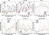 |
Fig. 6. Zoom-in on the details of the normalized spectral time series of SN 2022xlp shown in Fig. 3 and described in Table D.1, focusing on characteristic spectral lines. The lines specified in the legend correspond to the different epochs observed. Note: to improve clarity, not all epochs are plotted. |
We also compared the spectra of four SNe from different luminosity groups of the Iax subclass at similar phases. All spectra obtained approximately 19 days after the explosion, thus relatively close to their peak luminosity, are plotted in Fig. 7 (when the characteristic IME spectral features can still be identified). There is a strong similarity between SN 2022xlp and SN 2019muj with respect to their continuum and spectral lines. Figure 7 shows that the photospheric temperature and, thus, the steepness of the continuum increase with the brightness of the supernova at the same epoch relative to the explosion. The characteristic spectral lines of the Iax SN sample can be compared by normalization of the spectra, which are plotted in Fig. 8. In the case of SN 2022xlp, the lines of IGE elements, namely Co II, Ni II, Ca II, and Cr II are stronger in the 3700−4750 Å range compared to SN 2019muj, which is a result of the difference in the density profile due to the difference in epochs between the two spectra. Above 4750 Å, we observe lines of approximately the same strength, such as Fe II, Co II, and Si II. In the case of the fainter SN 2022ywf, the Na I D line is stronger than in either of the other supernovae; this is also the case for the Fe II, Ni II, and O I lines in the 7300−7700 Å range, as well as the Ca II and Co II lines in the 8300−8700 Å range. The more luminous SN 2012Z shows the same set of lines in the 3500−5400 Å wavelength range. The Si II λ6355 line is the weakest in this supernova sample, while the Na I D cannot be identified. The prominent appearance of Na I D and Si II λ6355 lines in the spectra of the fainter SNe Iax suggest either a lower ejecta temperature or an enhancement of the IMEs. In general, the appearance of these spectral features indicates similar abundance profiles but a faster evolution of the fainter SNe Iax. These differences may possibly arise from the steepness of their density profiles. An alternative explanation is that SNe Iax have similar temperature profiles, but the abundance profiles are stratified; at the same time, after the explosion, the photosphere is located at a different layer. However, the pure deflagration hydrodynamic simulations do not support a stratified abundance profile scenario.
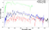 |
Fig. 7. Spectra of SN 2022xlp, SN 2019muj (Barna et al. 2021), SN2012Z (Stritzinger et al. 2015), and SN 2022ywf (Barna et al. in prep.) measured 19 days after the explosion. Because of the order of magnitude difference in luminosity in the Iax subclass, we plot the logarithm of spectral luminosity density. The strong similarity between SN 2022xlp and SN 2019muj can be amply observed. |
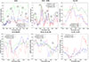 |
Fig. 8. Normalized spectra of the Iax-type supernovae SN 2019muj (Barna et al. 2021), the intermediate-luminous SN 2022xlp, bright SN 2012Z (Stritzinger et al. 2015), and faint SN 2022ywf (Barna et al. in prep.) in the wavelength range of the characteristic P-Cygni spectral lines. Note: the S/N of the spectra of SN 2012Z is too low above ∼ 8000 Å and thus it is not plotted in the lower right subplot. |
We performed a detailed spectral tomography analysis on the spectral time series of SN 2022xlp to determine the physical and abundance structure of the ejecta. In a co-moving frame, the photosphere moves inward with time as the ejecta expands and the temperature decreases. Thus, deeper and deeper ejecta regions gradually become part of the optically thin atmosphere and the strongest line-forming region. By comparing spectra taken at different epochs, we can determine the radial profiles of the physical properties and abundances via the fittings with synthetic spectra calculated by a radiative transfer code. This method is called spectral tomography. We used a Monte Carlo-based 1D radiative transfer code TARDIS (Kerzendorf & Sim 2014) to synthesize the theoretical model spectra. The model parameters kept fixed during the fitting are presented in Appendix E. The self-consistent fitting of spectra time series with TARDIS-synthesized spectra allowed us to reveal the SN ejecta’s radial density and abundance profile. The parameters of these profiles must be specified at a reference time and kept constant for all epochs. This is because the slope of the density profile and the abundances of the stable isotopes do not change over time; in addition, the code calculates the expansion-caused dilution together with the radioactive decay of unstable isotopes. By comparing the parameters determined from spectral tomography with those modelled from the pure deflagration explosion simulations, we can estimate the possible explosion process and the progenitor object of the supernova.
One of the most important sources of information regarding the outermost regions of the ejecta is the pre-maximum spectrum and its TARDIS model fitting, which can be seen in the upper left subplot of Fig. 9. It was observed 4.7 days and 6.2 days before the maximum brightness of the B and V bands and 6 days after the explosion date constrained in the spectral tomography analysis. The first spectrum shows only a few relatively weak spectral lines; thus, it offers the best opportunity to determine the characteristic value of continuum-related physical quantities. The determined bolometric luminosity is L(texp = 6.0 days) = 1.58 × 10⁸ L⊙, while the photospheric velocity is vphot(texp = 6.0 days) = 5400 km/s. The physical properties of the ejecta determined by spectral tomography are summarized in Table 4 for all epochs. The strongest lines can be identified at shorter wavelengths between 4100 − 5100 Å, and belong to highly ionized IGE-s, mainly, Fe III, Co III, and Ni II. There are some signs of IME-s, such as S III around 4225 Å, Si III at 4529 Å, and C II around 4670 Å, 6580 Å and 7170 Å. The highly ionised ions and the steep, blue-dominated continuum show high photospheric temperature. According to the fitted model spectra, the photospheric temperature was Tphot(texp = 6.0 days) = 11870 K. The Si II λ6355 line is clearly detectable. The effects of the Thomson-scattering and the bound-bound transitions of different ions can be visualized in a so-called spectral decomposition (SDEC) plot, shown in Fig. 10. The SDEC plot of the first epoch presents the dominance of Ni, Co, and Fe ions in the spectra, as we would expect from the hydrodynamic deflagration simulations (see models from, e.g., Lach et al. 2022 or Fink et al. 2014). Due to the lack of very early-phase photometric data, we were unable to determine the explosion time using the expanding fireball method, so we treated it as a fitting parameter during the spectral fitting process to obtain this parameter.
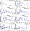 |
Fig. 9. Spectra time series fittings of SN 2022xlp with TARDIS-synthesised model spectra. The figure also shows the identified spectral lines at the two highlighted epochs: a post- and near maximum and a late-phase spectrum. The phase relative to the V-band maximum and the time since the explosion are also marked. |
Physical properties of the SN 2022xlp ejecta constrained in fitting the spectral series with TARDIS.
The next spectrum of the time series was measured 19.0 days after the explosion, as well as 8.0 days and 6.5 days after the B and V maximum, respectively. Compared with the spectrum of the previous epoch, it shows stronger lines over the whole wavelength range. The most prominent line-forming IGE ions are Co II, Ni II, Fe II, and Cr II; while the Ca II, Si II és O I lines from IME also have significant features, especially in the red part of the spectrum. The Ca II also has an effect on the blue part and Mg II contributes to a spectral line above 9000 Å. The observed and fitted synthetic spectra are plotted in the top right panel of Fig. 9. With the decrease in photospheric temperature, the Si IIλ6355 line emerged more prominently. According to the best-fit TARDIS model spectrum, the photospheric temperature was Tphot(texp = 19.0 days) = 6937 K, its velocity vphot(texp = 19.0 days) = 4400 km/s, while the luminosity L(texp = 19.0 days) = 1.58 × 10⁸ L⊙. We also measured the photospheric velocity by fitting the Si II λ6355 line, which is a widely used method for thermonuclear SNe. In case of type Iax SNe, however, Si II λ6355 is often blanketed by Fe II λ6456 and by Co II lines, which may lead to the underestimation of vphot when applying a single Gaussian profile to fit the observed absorption feature Szalai et al. (2015). Therefore, we also adopted a double Gaussian function to account for the presence of any other lines next to Si II λ6355. This method provides vphot, Gauss(texp = 19.0 days) = 2570 km/s, which is still a significantly lower value than that of the spectral tomography. Since radiative transfer modeling offers a more physical approach and, thus, more accurate velocity estimation is expected, we accept and use vphot(texp = 19.0 days) = 4400 km/s constrained by spectral synthesis hereafter. The SDEC plot of this near-maximum epoch can be seen in Fig. 10, which still shows significant Ni, Co, and Fe spectral features.
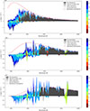 |
Fig. 10. The spectral decomposition (SDEC) plots of SN 2022xlp at texp = 6.0 days (top), texp = 19.0 days (middle) and texp = 73.0 days (bottom). The figures show the synthetic model spectrum and also the contribution of various light-matter interactions and elements to the spectrum, indicating how much they add or subtract from the spectral luminosity density at different wavelengths. The red dashed line represents the Planck curve corresponding to the photospheric temperature. |
The fit of the next four spectra in the time series can be seen in the two middle rows of Fig. 9. The phases and the time since the explosion are listed in Table D.1, while the determined time-dependent physical parameters, such as the photospheric velocity and temperature, as well as the bolometric luminosity, are summarized in Table 4. The synthetic spectrum agrees well with the observed spectrum below 6600 Å. Above this wavelength, the model continuum overestimates the observed spectrum, which is caused either by the uncertainty of photospheric properties or the presence of unidentified absorption features. The spectral luminosity density decreases monotonically after the maximum, with an initially faster rate of decline. Similar conclusions can be drawn regarding the photospheric temperature and velocity. In the shorter wavelength part of the spectrum, below 5500 Å, the main line-forming ions from the IGE elements are Co II, Fe II, and Ni II, while from the IME elements are Cr II, Ca II, and Si II. The strength of the Ni feature decreases with time due to the radioactive decay of 56Ni. On the red side of the spectrum, above 5500 Å, the line-forming ions are Na I, Fe II, Cr II, Si II, Ca II, and Mg II. A detectable line is also produced by O I around ∼ 7750 Å, as well as a significant line triplet by Ca II near ∼ 8830 Å, which strengthens over time. As time progresses after the explosion, the spectrum becomes increasingly dominated by Fe II ion lines, and the Na I D line also becomes more prominent due to the temperature decrease in the atmospheric layers. Some spectral lines in the 6650−7320 Å range, as well as those near ∼ 9760 Å, could not be fitted. The presence of these lines likely requires modification of the abundance profile adopted from deflagration models used for comparison, requiring adjustments to the abundances of certain isotopes (introduced at the end of thissection).
We used two of the last four observed spectra of SN 2022xlp for our spectral tomography, since the late-phase evolution of thermonuclear SNe is slower than in the early phase. These late-time spectra were obtained at texp = 73.0 days and texp = 102.8 days after the explosion (60.4 days and 90.5 days after the V-band maximum). The observed and fitted model spectra are plotted in Fig. 9. By this time, the spectrum is dominated by Fe I and Fe II lines throughout the optical regime. The only noticeable contributions of IMEs are the Na I D line, the Ca II NIR triplet, and the O I λ7770 feature. At shorter wavelengths, there are weak P Cygni profiles of Ca II, Cr II, and Co II ions. The contributions of Cr II and O I ions nearly disappear 102.8 days after the explosion. Beyond 6600 Å, the continuum flux of the synthetic spectrum is higher than that of the observed spectrum and fitting the observed spectral features between 6600−7360 Å, 7780−8310 Å and above 8910 Å was not feasible with our TARDIS model. A possible explanation of this discrepancy in the 7000−7500 Å region is the rise of forbidden emission lines in the late phase spectrum, described in Foley et al. (2016a). Forbidden emissions are significant at 102.8 days (prior to this, the growing forbidden lines are difficult to distinguish from the previously existing P Cygni features), where we can see some narrow and strong emission lines in the red part of the spectrum. According to the discussion of Foley et al. (2016a), the Fe II λ7155, Ca II λ7291, Ca II λ7324, and Ni II λ7378 lines are the strongest forbidden emission lines. The appearance of these emission features is made possible by the significant dilution of the outer layers of the supernova ejecta; however, the TARDIS code is unable to synthesize these lines. Thus, we simply omitted these emission features from our fitting process. However, based on TARDIS fits, the Fe II λ7465 line appears, which is not a forbidden emission line at least at 73.0 days after the explosion. The photospheric velocity has also decreased to vphot(texp = 73.0 days) = 800 km s−1 and further decreased to vphot(texp = 102.8 days) = 565 km s−1, while the photospheric temperature has also changed to Tphot(texp = 73.0 days) = 4803 K and Tphot(texp = 102.8 days) = 4475 K. The bolometric luminosity has reached L(texp = 73.0 days) = 2.34 × 10⁷ L⊙ and L(texp = 102.8 days) = 1.82 × 10⁷ L⊙. The SDEC plot of this epoch can be seen in Fig. 10, which shows exclusively Fe-dominated spectra and the significant Na I D and Ca II NIR triplet features.
From the various pure deflagration models of Fink et al. (2014) and Lach et al. (2022), we selected those exhibiting a peak luminosity and bolometric LC roughly similar to those of SN 2022xlp. The most similar models are def_2021_r48_d5.0_z and def_2021_r120_d5.0_z from Lach et al. (2022) with peak bolometric absolute magnitudes of Mbol, peak(def_2021_r48_d5.0_z) = − 15.83 mag and Mbol, peak(def_2021_r120_d5.0_z) = − 15.38 mag. We adopted the abundance profile of model def_2021_r48_d5.0_z for the spectral synthesis with TARDIS, but allowed for minor modifications to further improve the fit. Regarding the density profile, we applied a custom model based on Barna et al. (2021) or Barna et al. (2018), which can be expressed as:
 (7)
(7)
where ρ0 is the core density at 100 s after the explosion, v0 describes the decrease in density outward the ejecta. The derived density profile, along with the adopted def_2021_r48_d5.0_z and minor-modified deflagration abundance profile, is shown in Fig. 11. The density profile of the def_2021_r48_d5.0_z model produces overly strong spectral lines at early epochs, as shown in Fig. 12, because it predicts excessively high densities in the layers above the photosphere. To improve the fit of synthetic spectra, we constrained a density function described by Eq. 7 instead, where the parameters are ρ0 = 0.4 g cm−3, while v0 = 3000 km s−1 (summarized in Table 4). Our fitted density profile introduces a steep cutoff of vlim = 4400 km s−1, beyond which the density declines more rapidly, resulting in a proper fit for the spectral lines. After the maximum, the spectra become less sensitive to the density profile, as is seen in Fig. 12. The slope of the constrained density profile differs from the density profiles estimated by the deflagration models def_2021_r48_d5.0z_ and def_2021_r120_d5.0_z. The slightly slower decline leads to more material being present before the cutoff point, and significantly less in the outermost regions of the ejecta beyond the cutoff. The synthetic spectra closer to the maximum brightness are more sensitive to the abundance profile, while the later spectra are dominated by iron lines and insensitive to the IMEs. The adopted abundance profile of the def_2021_r48_d5.0_z deflagration model results in a very good fit to the series of spectra, except for the Na I D line. This line could be fit only by significantly increasing the Na abundance to 0.06 in all layers, while correspondingly decreasing the O abundance, which has a relatively weaker effect. The spectra calculated with the density and abundance profile of the def_2021_r48_d5.0_z model are shown with our fitted spectra in Fig. 12. Here, we can see that the Na I D line cannot be fit with the abundance profile of the def_2021_r48_d5.0_z model.
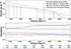 |
Fig. 11. Density and abundance profiles obtained from the tomographic analysis of SN 2022xlp. Vertical lines on the density profile indicate its sampling points. The blue and green dashed lines show the density profiles of the def_2021_r48_d5.0_z and def_2021_r120_d5.0_z models. The abundance profile is identical to that of the def_2021_r48_d5.0_z deflagration model, except for an increased Na abundance and a corresponding reduction in O abundance. |
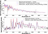 |
Fig. 12. Comparison of the model spectra of SN 2022xlp at different epochs. The model spectra calculated with the fitted density and Na-corrected abundance profile are shown with blue curves. In contrast, the spectra computed using exactly the adopted density and abundance profiles of the def_2021_r48_d5.0_z model are shown with red curves. Apart from the density and abundance profiles, the values of the other parameters are identical at each epoch. |
6. Summary and conclusions
We present our multicolor photometric and spectroscopic observations of SN 2022xlp, which is the second intermediate-luminosity type Iax SN with detailed follow-up, as its V-band LC peaks at Mmax(V) = − 16.04 ± 0.25 mag. The data set starts at 6.0 days and covers ∼73.0 days after the explosion. Based on observing characteristics, such as LC properties, color evolution, and spectral features, SN 2022xlp is shown to be very similar to SN 2019muj, bridging the luminosity gap of the diverse Iax class. The change in color-indexes is ∼1.5 mag between −8.0 and 20.0 days, indicating a rapidly decreasing photospheric temperature. After 20 days the V-band maximum, the B–V and r–i colors are almost constant, while g-r and g–i show a slow decline. By comparing the color evolution of various luminous SNe Iax, we can conclude that the amplitude of the color change is greater in the case of brighter Iax supernovae.
We performed a semi-bolometric LC fitting based on the Arnett model to set constraints on the general parameters of the ejecta. The results of the modeling are MNi = 0.012 ± 0.009 M⊙ for the nickel mass, Mej = 0.142 ± 0.015 M⊙ for the ejecta mass, and Ekin = (2.066 ± 0.236)×1049 erg for the kinetic energy. Based on the synthetic LC fitting, the Ni mass, ejecta mass, explosion energy, and effective diffusion time are similar to those of SN 2019muj. According to the bolometric LC analysis of SNe 2019muj and 2022xlp, the characteristic mass parameters of the intermediate luminous SNe Iax are MNi ∼ 0.02 − 0.03 M⊙ and Mej ∼ 0.09 − 0.17 M⊙. We performed a comprehensive spectroscopic analysis that included a qualitative comparison of the spectra of different SNe Iax with different peak luminosities, a spectral line evolution study, and detailed spectral tomography. The main results are listedbelow.
-
Based on the analysis of the evolution of spectral features:
-
After the maximum, the widths of the IGE spectral lines at the 3600−4400 Å wavelength range indicate a widening of the line-forming regions of IGEs, along with quasi-constant abundances. This result shows good agreement with pure deflagration hydrodynamic simulation results.
-
The increasing strength of the Na I D lines indicates a high Na abundance (X(Na)≃0.05) in the outermost region of the ejecta, compared to the predictions of pure deflagration models.
-
-
Based on the comparison of the spectra of different SNe Iax at the same time since explosion:
-
There is a strong similarity between SN 2022xlp and SN 2019muj.
-
The prominent appearance of Na I D and Si II λ6355 lines in the spectra of fainter SNe Iax suggest a lower photospheric temperature profile in the case of fainter Iax supernovae. These spectral features also indicate similar abundance profiles.
-
The fainter SNe Iax evolve faster. Their temperature profile decreases faster or the decline starts at lower temperatures. The difference in the evolution rate can possibly originate from the difference in the density profile.
-
-
Based on the spectral tomography:
-
The physical quantities characteristic of the ejecta, the luminosity, the photospheric temperature, and the velocity could be determined by fitting the observed spectra time series with the TARDIS synthesized spectra. These results are summarized in Table 4.
-
We present the line identification results at the most important epochs, the first post-maximum spectra, and the latest spectra (see Fig. 9, and Fig. 10).
-
The density profile could be determined and compared with the results of the most similar pure deflagration hydrodynamic simulations (see Fig. 11). The most important result is that the determined density profile differs in its rate of decline from the density profiles calculated by the deflagration hydrodynamic simulations def_2021_r48_d5.0_z and def_2021_r120_d5.0_z. Our fitted density profile introduces a steep cutoff resulting significantly lower densities in the outermost regions to prevent the presence of excessively strong lines at the early epochs.
-
The adopted abundance profile of the def_2021_r48_d5.0_z deflagration model results in a very good fit to the series of spectra, except for the Na I D line. This line can only be well fitted by significantly increasing the Na abundance in all layers, while correspondingly decreasing the O abundance, which has a relatively smaller effect.
-
In summary, SN 2022xlp shows a very strong similarity to the first, well-analyzed intermediate-luminous Iax supernova, SN 2019muj. SN 2022xlp supports the assumption of the luminosity-velocity relation bridging the previously existing luminosity gap together with SN 2019muj. For a more detailed recognition of the intermediate-luminous range of SNe Iax, further analyses and even more objects would be required.
Data availability
All spectra are available at the WISeREP (Yaron & Gal-Yam 2012) online supernova database: https://www.wiserep.org/object/21831.
NED can be accessed at https://ned.ipac.caltech.edu/
The official website of the LCO can be accessed at https://lco.global/
The official website of the LCO can be accessed at https://lco.global/
Detailed description of the instrument can be found at https://lco.global/observatory/instruments/floyds/
Detailed description of FLOYDS pipeline is available at https://github.com/svalenti/FLOYDS_pipeline
The Pan-STARRS DR1 archive: https://outerspace.stsci.edu/display/PANSTARRS/
Acknowledgments
This work was supported by the professional funding from the University Research Scholarship Programme (project code: EKÖP-24-3-SZTE-484) of the Ministry of Culture and Innovation, financed by the National Research, Development, and Innovation Fund (NKFIH), Hungary. The deployment and operation of the BRC80 telescope was supported by the GINOP 2.3.2-15-2016-00033 project of the NKFIH and the Hungarian Government, funded by the European Union. JV is supported by the NKFIH-OTKA grant K142534. The UCSC team is supported in part by NASA grant 80NSSC20K0953, NSF grant AST–1815935, and by a fellowship from the David and Lucile Packard Foundation to R.J.F. A major upgrade of the Kast spectrograph on the Shane 3 m telescope at the Lick Observatory was made possible through generous gifts from the Heising–Simons Foundation as well as William and Marina Kast. Research at the Lick Observatory is partially supported by a generous gift from Google. Supernova research at Rutgers University is supported in part by US NSF award AST-2407567 to S.W.J. IRAF is distributed by NOAO, which is operated by AURA, Inc., under cooperative agreement with the NSF. L.G. acknowledges financial support from AGAUR, CSIC, MCIN and AEI 10.13039/501100011033 under projects PID2023-151307NB-I00, PIE 20215AT016, CEX2020-001058-M, and 2021-SGR-01270. This project has received funding from the HUN-REN Hungarian Research Network. I. B. B. acknowledge the financial support of the Hungarian National Research, Development and Innovation Office – NKFIH Grants K-147131 and K-138962.
References
- Arnett, W. D. 1982, ApJ, 253, 785 [Google Scholar]
- Barna, B., Szalai, T., Kerzendorf, W. E., et al. 2018, MNRAS, 480, 3609 [NASA ADS] [CrossRef] [Google Scholar]
- Barna, B., Szalai, T., Jha, S. W., et al. 2021, MNRAS, 501, 1078 [Google Scholar]
- Branch, D., Dang, L. C., Hall, N., et al. 2006, PASP, 118, 560 [NASA ADS] [CrossRef] [Google Scholar]
- Burrows, D. N., Hill, J. E., Nousek, J. A., et al. 2005, Space Sci. Rev., 120, 165 [Google Scholar]
- Chatzopoulos, E., Wheeler, J. C., & Vinko, J. 2012, ApJ, 746, 121 [Google Scholar]
- Chatzopoulos, E., Wheeler, J. C., Vinko, J., Horvath, Z. L., & Nagy, A. 2013, ApJ, 773, 76 [NASA ADS] [CrossRef] [Google Scholar]
- Coulter, D. A., Jones, D. O., McGill, P., et al. 2022, https://doi.org/10.5281/zenodo.7278430 [Google Scholar]
- Coulter, D. A., Jones, D. O., McGill, P., et al. 2023, PASP, 135, 064501 [Google Scholar]
- Fink, M., Kromer, M., Seitenzahl, I. R., et al. 2014, MNRAS, 438, 1762 [NASA ADS] [CrossRef] [Google Scholar]
- Firth, R. E., Sullivan, M., Gal-Yam, A., et al. 2015, MNRAS, 446, 3895 [NASA ADS] [CrossRef] [Google Scholar]
- Foley, R. J., Papenkova, M. S., Swift, B. J., et al. 2003, PASP, 115, 1220 [NASA ADS] [CrossRef] [Google Scholar]
- Foley, R. J., Chornock, R., Filippenko, A. V., et al. 2009, AJ, 138, 376 [NASA ADS] [CrossRef] [Google Scholar]
- Foley, R. J., Jha, S. W., Pan, Y.-C., et al. 2016a, MNRAS, 461, 433 [NASA ADS] [CrossRef] [Google Scholar]
- Foley, R. J., Pan, Y.-C., Brown, P., et al. 2016b, MNRAS, 461, 1308 [Google Scholar]
- Ganeshalingam, M., Li, W., Filippenko, A. V., et al. 2012, ApJ, 751, 142 [NASA ADS] [CrossRef] [Google Scholar]
- Gehrels, N., Chincarini, G., Giommi, P., et al. 2004, ApJ, 611, 1005 [Google Scholar]
- Guttman, O., Shenhar, B., Sarkar, A., & Waxman, E. 2024, MNRAS, 533, 994 [Google Scholar]
- Horne, K. 1986, PASP, 98, 609 [Google Scholar]
- Itagaki, K. 2022, Transient Name Server Discovery Report, 2022–2971, 1 [Google Scholar]
- Jha, S. W. 2017, in Handbook of Supernovae, eds. A. W. Alsabti, & P. Murdin, 375 [Google Scholar]
- Johnson, H. R. 1964, Ann. Astrophys., 27, 695 [Google Scholar]
- Kerzendorf, W. E., & Sim, S. A. 2014, MNRAS, 440, 387 [NASA ADS] [CrossRef] [Google Scholar]
- Kromer, M., Ohlmann, S. T., Pakmor, R., et al. 2015, MNRAS, 450, 3045 [NASA ADS] [CrossRef] [Google Scholar]
- Lach, F., Callan, F. P., Bubeck, D., et al. 2022, A&A, 658, A179 [NASA ADS] [CrossRef] [EDP Sciences] [Google Scholar]
- Li, W., Filippenko, A. V., Chornock, R., et al. 2003, PASP, 115, 453 [Google Scholar]
- Long, M., Jordan, G. C. I., van Rossum, D. R., et al. 2014, ApJ, 789, 103 [NASA ADS] [CrossRef] [Google Scholar]
- Magee, M. R., Kotak, R., Sim, S. A., et al. 2016, A&A, 589, A89 [NASA ADS] [CrossRef] [EDP Sciences] [Google Scholar]
- McClelland, C. M., Garnavich, P. M., Galbany, L., et al. 2010, ApJ, 720, 704 [NASA ADS] [CrossRef] [Google Scholar]
- Miller, J. S., & Stone, R. P. S. 1993, Lick Obs. Tech. Rep., 66 [Google Scholar]
- Milne, P. A., Brown, P. J., Roming, P. W. A., et al. 2010, ApJ, 721, 1627 [Google Scholar]
- Narayan, G., Foley, R. J., Berger, E., et al. 2011, ApJ, 731, L11 [NASA ADS] [CrossRef] [Google Scholar]
- Nicholl, M. 2018, Res. Notes Am. Astron. Soc., 2, 230 [NASA ADS] [Google Scholar]
- Pál, A. 2012, MNRAS, 421, 1825 [Google Scholar]
- Phillips, M. M. 1993, ApJ, 413, L105 [Google Scholar]
- Pskovskii, I. P. 1977, Sov. Ast., 21, 675 [NASA ADS] [Google Scholar]
- Rodríguez, Ó., Clocchiatti, A., & Hamuy, M. 2014, AJ, 148, 107 [CrossRef] [Google Scholar]
- Roming, P. W. A., Kennedy, T. E., Mason, K. O., et al. 2005, Space Sci. Rev., 120, 95 [Google Scholar]
- Siebert, M. R., Dimitriadis, G., Polin, A., & Foley, R. J. 2020, ApJ, 900, L27 [NASA ADS] [CrossRef] [Google Scholar]
- Silverman, J. M., Foley, R. J., Filippenko, A. V., et al. 2012, MNRAS, 425, 1789 [Google Scholar]
- Singh, M., Sahu, D. K., Barna, B., et al. 2024, ApJ, 965, 73 [NASA ADS] [CrossRef] [Google Scholar]
- Srivastav, S., Smartt, S. J., Leloudas, G., et al. 2020, ApJ, 892, L24 [NASA ADS] [CrossRef] [Google Scholar]
- Stritzinger, M. D., Hsiao, E., Valenti, S., et al. 2014, A&A, 561, A146 [NASA ADS] [CrossRef] [EDP Sciences] [Google Scholar]
- Stritzinger, M. D., Valenti, S., Hoeflich, P., et al. 2015, A&A, 573, A2 [NASA ADS] [CrossRef] [EDP Sciences] [Google Scholar]
- Szalai, T., Vinkó, J., Sárneczky, K., et al. 2015, MNRAS, 453, 2103 [NASA ADS] [CrossRef] [Google Scholar]
- Taguchi, K., Maeda, K., & Kawabata, M. 2022, Transient Name Server Classification Report, 2022–2999, 1 [Google Scholar]
- Tomasella, L., Cappellaro, E., Benetti, S., et al. 2016, MNRAS, 459, 1018 [NASA ADS] [CrossRef] [Google Scholar]
- Tonry, J. L., Stubbs, C. W., Lykke, K. R., et al. 2012, ApJ, 750, 99 [Google Scholar]
- Valenti, S., Benetti, S., Cappellaro, E., et al. 2008, MNRAS, 383, 1485 [Google Scholar]
- Yaron, O., & Gal-Yam, A. 2012, PASP, 124, 668 [Google Scholar]
Appendix A: Multicolor photometric data reduction
In this appendix, we present the detailed multicolor photometric data reduction process used at the Baja Astronomical Observatory of the University of Szeged. The images taken on the same night with the same color filter are averaged to improve the signal-to-noise ratio and the limit magnitude. The instrumental magnitudes of the SN are calculated by the image subtraction method. The essence of this method is to subtract a pre-supernova template image of the galaxy’s environment from the supernova images. This template image is properly scaled in size, flux, and in the full width at half maximum (FWHM) of the star profiles’ PSF with the geomap, gregister, psfmatch and linmatch IRAF tasks. As a result, the galaxy and the stars in the field of view disappear, leaving only the supernova, which can then be easily measured using aperture photometry. We used Pan-STARRS DR1 images as templates. Finally, using the SDSS band photometric standard stars from Pan-STARRS DR17 on the original unsubtracted images, the photometric standard transformation can easily be performed. The selection of the photometry reference stars and the calibration procedures are done in four steps. First, sources within a 5 arcmin radius around the SN with r-band brightness between 15 and 17 mag are downloaded from the PS1 database. In the second step, we should sort out the non-stellar sources based on the criterion iPSFmag − iKronmag < 0.05 for stars. To obtain reference magnitudes for Johnson-Cousins-Bessel B and V-band, the PS1 magnitudes are transformed into the BVRI system based on equations and coefficients in (Tonry et al. 2012). Finally, instrumental magnitudes are transformed into standard magnitudes by applying a linear color correction term (g – i) and wavelength-dependent zero points. An atmospheric extinction correction is not necessary because the reference stars fall close to the supernova around in a few arcminutes.
Exposure time by filters used at the BRC80 telescope.
Appendix B: Multicolor photometric data
Long-term multicolor photometric follow-up data of SN 2022xlp transformed to the standard system.
Appendix C: UV photometry
UV photometric dataset measured by the Swift Ultraviolet/Optical Telescope (UVOT).
Appendix D: The log of spectral observations
Log of the observed spectra of SN 2022xlp.
Appendix E: Fixing the model parameters of TARDIS simulations
Configuration of TARDIS simulations used to fit the measured spectra with the synthesized spectra.
All Tables
Physical properties of the SN 2022xlp ejecta constrained in fitting the spectral series with TARDIS.
Long-term multicolor photometric follow-up data of SN 2022xlp transformed to the standard system.
UV photometric dataset measured by the Swift Ultraviolet/Optical Telescope (UVOT).
Configuration of TARDIS simulations used to fit the measured spectra with the synthesized spectra.
All Figures
|
Fig. 1. Image of NGC 3938 hosted the SN 2022xlp. This picture was taken with the BRC80 telescope in the Baja Astronomical Observatory of the University of Szeged. |
| In the text | |
|
Fig. 2. Ground-based photomety of SN 2022xlp. The zoom-inset highlights the near-maximum observations. Data measured by the BRC80 telescope are marked with triangles, while filled circles mark the LCO data points. |
| In the text | |
|
Fig. 3. Optical spectra of SN 2022xlp. The characteristic spectral features are highlighted by gray stripes. The phase relative to the V-band maximum (tV) and the time since the explosion (texp) are also marked. |
| In the text | |
|
Fig. 5. Evolution of different color indexes compared to another SNe Iax (SN 2019muj – (Barna et al. 2021), SN 2012Z – (Stritzinger et al. 2015), and SN 2008ha – (Foley et al. 2009; Stritzinger et al. 2014)). SN 2022xlp shows a very similar color evolution to SN 2019muj. The color indexes are corrected for the extinction as described in Sect. 4. We adopted the color excess from the papers listed above. |
| In the text | |
|
Fig. 4. Pseudo-bolometric LC of SN 2022xlp and the best-fit synthetic light model. |
| In the text | |
|
Fig. 6. Zoom-in on the details of the normalized spectral time series of SN 2022xlp shown in Fig. 3 and described in Table D.1, focusing on characteristic spectral lines. The lines specified in the legend correspond to the different epochs observed. Note: to improve clarity, not all epochs are plotted. |
| In the text | |
|
Fig. 7. Spectra of SN 2022xlp, SN 2019muj (Barna et al. 2021), SN2012Z (Stritzinger et al. 2015), and SN 2022ywf (Barna et al. in prep.) measured 19 days after the explosion. Because of the order of magnitude difference in luminosity in the Iax subclass, we plot the logarithm of spectral luminosity density. The strong similarity between SN 2022xlp and SN 2019muj can be amply observed. |
| In the text | |
|
Fig. 8. Normalized spectra of the Iax-type supernovae SN 2019muj (Barna et al. 2021), the intermediate-luminous SN 2022xlp, bright SN 2012Z (Stritzinger et al. 2015), and faint SN 2022ywf (Barna et al. in prep.) in the wavelength range of the characteristic P-Cygni spectral lines. Note: the S/N of the spectra of SN 2012Z is too low above ∼ 8000 Å and thus it is not plotted in the lower right subplot. |
| In the text | |
|
Fig. 9. Spectra time series fittings of SN 2022xlp with TARDIS-synthesised model spectra. The figure also shows the identified spectral lines at the two highlighted epochs: a post- and near maximum and a late-phase spectrum. The phase relative to the V-band maximum and the time since the explosion are also marked. |
| In the text | |
|
Fig. 10. The spectral decomposition (SDEC) plots of SN 2022xlp at texp = 6.0 days (top), texp = 19.0 days (middle) and texp = 73.0 days (bottom). The figures show the synthetic model spectrum and also the contribution of various light-matter interactions and elements to the spectrum, indicating how much they add or subtract from the spectral luminosity density at different wavelengths. The red dashed line represents the Planck curve corresponding to the photospheric temperature. |
| In the text | |
|
Fig. 11. Density and abundance profiles obtained from the tomographic analysis of SN 2022xlp. Vertical lines on the density profile indicate its sampling points. The blue and green dashed lines show the density profiles of the def_2021_r48_d5.0_z and def_2021_r120_d5.0_z models. The abundance profile is identical to that of the def_2021_r48_d5.0_z deflagration model, except for an increased Na abundance and a corresponding reduction in O abundance. |
| In the text | |
|
Fig. 12. Comparison of the model spectra of SN 2022xlp at different epochs. The model spectra calculated with the fitted density and Na-corrected abundance profile are shown with blue curves. In contrast, the spectra computed using exactly the adopted density and abundance profiles of the def_2021_r48_d5.0_z model are shown with red curves. Apart from the density and abundance profiles, the values of the other parameters are identical at each epoch. |
| In the text | |
Current usage metrics show cumulative count of Article Views (full-text article views including HTML views, PDF and ePub downloads, according to the available data) and Abstracts Views on Vision4Press platform.
Data correspond to usage on the plateform after 2015. The current usage metrics is available 48-96 hours after online publication and is updated daily on week days.
Initial download of the metrics may take a while.