| Issue |
A&A
Volume 703, November 2025
|
|
|---|---|---|
| Article Number | A293 | |
| Number of page(s) | 15 | |
| Section | Stellar structure and evolution | |
| DOI | https://doi.org/10.1051/0004-6361/202553975 | |
| Published online | 01 December 2025 | |
V1001 Cen: A dual approach of spectroscopy and numerical modeling to understand stellar evolution and dynamo mechanisms
1
Departamento de Astronomía, Universidad de Concepción, Casilla 160-C, Concepción, Chile
2
Dipartimento di Fisica, Sapienza, Universita di Roma, Piazzale Aldo Moro 5, I-00185 Roma, Italy
3
Astronomical Observatory, Volgina 7, 11060 Belgrade 38, Serbia
4
Isaac Newton Institute of Chile, Yugoslavia Branch, 11060 Belgrade, Serbia
⋆ Corresponding author: This email address is being protected from spambots. You need JavaScript enabled to view it.
Received:
31
January
2025
Accepted:
14
August
2025
Abstract
This study aims to determine the fundamental parameters of the binary system V1001 Cen, which remain poorly constrained. We conducted a photometric and spectroscopic study in the visual band of V1001 Cen, a system comprising two stellar components. Using Djurašević’s models, we derived the physical parameters of both stars, the accretion disk around the gainer star, and the system’s overall dimensions. Spectroscopic data from the CHIRON spectrometer allowed us to estimate the effective temperatures, semi amplitudes of radial velocity, and component masses. Disentangling the spectra using the Gonzalez & Levato (2006, A&A, 448, 283) technique provided additional details about the stellar components. Evolutionary models were generated using the MESA code, and comparisons with Van Rensbergen’s models were used to assess the system’s evolutionary stage. The orbital period of V1001 Cen was determined to be 6.73 ± 0.01 days, with a long period of 247.28 ± 10.0 days. The color excess was estimated as E(B − V) = 0.6351 ± 0.0292 mag. Semi amplitudes of radial velocity were measured at 21.70 ± 0.38 km s−1 and 142.33 ± 0.34 km s−1. The effective temperatures, determined using the spectrum code, are 8 750 ± 250 K for the donor star and 20 000 ± 2000 K for the gainer star. Masses were found to be 0.85 ± 0.1 M⊙ and 4.25 ± 0.1 M⊙ for the donor and gainer, respectively. The system, with an estimated age of 190 million years, is in its second phase of mass transfer, nearly conservative, with Ṁ = 1.13 × 10⁻⁷ M⊙ yr−1. Mass transfer began 58 million years ago. The best fitting light curve model indicates an inclination angle of i = 68.° 3 ± 0.° 3, Rg = 2.68 ± 0.1 R⊙, Rd = 6.47 ± 0.1 R⊙, Tg = 18 310 ± 500 K, and Td = 8750 ± 250 K, parameters belonging to the gainer and donor, respectively.
Key words: binaries: eclipsing / binaries: general / binaries: symbiotic / stars: evolution
© The Authors 2025
 Open Access article, published by EDP Sciences, under the terms of the Creative Commons Attribution License (https://creativecommons.org/licenses/by/4.0), which permits unrestricted use, distribution, and reproduction in any medium, provided the original work is properly cited.
This article is published in open access under the Subscribe to Open model. This email address is being protected from spambots. You need JavaScript enabled to view it. to support open access publication.
1. Introduction
Most stars in the Universe exist as binaries or multiple systems, making the study of binary star evolution crucial for understanding stellar populations. V1001 Cen, also known as HD 125104 and ASAS 141909-5552.9, has coordinates of α2000 = 14h 19m 09s, δ2000 = −55° 52′ 56″, with an apparent visual magnitude of 7.30 ± 0.02 mag and a B − V color index of 0.066 ± 0.054 mag. Classified as an eclipsing binary, this little studied system has an orbital period of 6.736 ± 0.003 days according to the ASAS-31 catalog (Pojmanski 2002), and is located in a region close to Alpha Centauri. Furthermore, V1001 Cen exhibits a long photometric cycle of 247 ± 3 days, and was reported as a double periodic variable (DPV) by Mennickent et al. (2016a). V1001 Cen is mentioned in that work as part of a larger set of objects studied in the context of interactive W Serpentids binaries and DPVs.
Double periodic variables are distinguished by their interacting binary behavior, manifesting a photometric variability that occurs on two time scales, a short orbital period associated with eclipses between stars and a long photometric cycle, approximately 33 times the orbital period, the origin is a topic under investigation (García et al. 2021). Mennickent (2022) and Mennickent & Kolaczkowski (2010) describe DPVs as intermediate mass binaries with optically thick disks around the accretor star. The primary more massive component is referred to as the gainer, and the less massive one as the donor. The interest of DPVs lies in their potential as natural laboratories for the study of the evolution of binary systems and the interaction between stellar components. The primary goal of this article is to provide a comprehensive characterization of the V1001 Cen system, including a theoretical model for its evolution. The article is organized as follows. Section 2 describes the photometric and spectroscopic analysis, which aims to determine the orbital and physical parameters of the system, such as temperatures, masses, periods, radial velocity, and spectral types for each component. In Section 3, we employ the stellar evolution code MESA (Paxton et al. 2015) to construct a range of models to estimate the current evolutionary phase of the system, as well as the mass and separation at which this binary system may have formed. Section 2.7 presents our conclusions throughout these sections.
2. Photometric and spectroscopic studies
2.1. Photometric data
To perform the photometric analysis of the V1001 Cen system, we used data from the all sky automated survey ASAS-3 (V filter). The All Sky Automated Survey, conceived by (Pojmanski 2002), is an astronomical project that uses multi pixel CCD detectors and has been instrumental in monitoring variable objects in the sky, including red giants and variable stars (Pojmański 2003). ASAS-3, in particular, is notable for its ability to observe the entire southern sky with two wide-field instruments and one narrow field one, collecting photometric data used for the study of binary systems and variable stars (Pojmański 2001). Furthermore, ASAS is a useful tool in the automated classification of periodic variable stars (Eyer & Blake 2002). This long term project has managed to discover 50 099 variables and 11 076 eclipsing binaries, contributing to the census of bright variable stars in the sky (Paczyński et al. 2006; Pigulski 2013). The ASAS public database has also been essential for the analysis of light curves of eclipsing binary systems, providing a good data source for research in this field (Ulaş & Ulusoy 2015).
To determine the period of the system, we first disentangled the light curve using software developed by Zbigniew Kolaczkowski and described in Mennickent et al. (2012a). This algorithm is based on fitting the data to a Fourier series, incorporating fundamental frequencies and their respective harmonics, which are identified in advance. The choice of the number of harmonics to be used is intrinsically linked to the morphology of the light curve. For example, in curves with sinusoidal patterns, the use of a few harmonics may be sufficient. However, given the inherent complexity of the light curves of eclipsing binary systems, the inclusion of a greater number of harmonics, typically on the order of 12 or more, is required for an accurate fit. Following the adjustment of the main light curve and its harmonics, the algorithm provides a set of residuals. These residuals are analyzed in the search for secondary frequencies associated with a second period.
We then used the Lomb scargle fast algorithm from the Python2 library gatspy periodic (VanderPlas & Ivezic 2015), this library extends the single band multiharmonic analysis of variance algorithm to estimate periods in multiple bands, improving period recovery rates by up to 50% (Mondrik et al. 2015). Furthermore, gatspy aggregates multidimensional and sparsely sampled time series information, which significantly increases the period retrieval rate (Huijse et al. 2018). We used gatspy to estimate the orbital period and the long period. The method extracts a periodic component with a specified frequency and leaves a residue curve that could show a second periodic component.
The orbital period was found to be Po = 6.73 ± 0.01 d. In addition, a long cycle of Pl = 247.19 ± 10.0 d was found, and is represented in Table 1. The light curves for each period reveal an orbital modulation typical of an ellipsoidal binary but with unequal maxima and a longer cycle characterized by quasi sinusoidal variability. Fig. 1 shows the light curve for the orbital period and the long period.
Orbital parameters for the donor or gainer star of V1001 Cen.
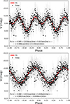 |
Fig. 1. Disentangled light curves from the ASAS data for the orbital period (Top) and long period (Bottom), phased between −1.0 and 1.0. The solid red line represents the best-fit function f(x) shown in the plot, and the gray lines represent the error bars. |
In the work of Mennickent et al. (2016a) the following ephemerides were reported for the light curve maxima of V1001 Cen:
 (1)
(1)
 (2)
(2)
But in our case the epochs found for the minimum of the light curve are:
 (3)
(3)
 (4)
(4)
In addition, from the photometric analysis to the ASAS data, we have determined other values, such as those in Table 2 showing the photometric aparent magnitudes in different filters extracted from the ExoFOP3 database. In turn, Fig. 1 shows the fitting of the light curves for the orbital period and the long period using a Fourier series. For the orbital period, the maximum magnitude of the curve is 7.34 ± 0.04 mag, the minimum is 7.26 ± 0.04 mag, and the total amplitude of the curve is 0.043 ± 0.003 mag. The detailed values of the parameters of the fitting functions for each case are specified in the footnotes of the corresponding figures.
Summary of photometric data for V1001 Cen.
2.2. Spectroscopic data
We obtained the spectra using the highly stable cross dispersion spectrometer CHIRON4 on the 1.5 m SMART telescope. A total of ten spectra were taken covering the orbital phase of the system. CHIRON is a fiber fed, Echelle type spectrometer with multiple observation modes that allow for spectral resolutions ranging from 28 000 to 120 000 (Schwab et al. 2012). This instrument is designed for high precision Doppler measurements using an iodine absorption cell and is optimized for monitoring the radial velocities of bright stars with high cadence and precision. For our observations, we used the high resolution mode, which provides a spectral resolution of R = 80 000, measured using a Thorium Argon calibration lamp. This mode delivers a broad spectral coverage from 410 to 870 nm, with an average signal to noise ratio (S/N) of ∼59 in our data. Fig. 2 shows the set of nine spectra centered at Hβ (4861.332 Å).
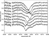 |
Fig. 2. Spectral dataset centered on the spectral line 6562.8, Å, obtained from cross dispersion spectrometer CHIRON. The orbital phase values of the spectra from top to bottom are 0.14, 0.23, 0.26, 0.43, 0.58, 0.70, 0.73, 0.84, 0.99. |
2.3. Radial velocity and spectral disentangling
To determine the radial velocity of each component of V1001 Cen, we first identified characteristic absorption lines that represent the individual motion of each star. For the donor star, which exhibits a wider orbital motion reflected in its absorption lines, we selected the Fe I line at 6677.993 Å (see Fig. 3, Table 3). For the other component, the accreting star, we used the Hα line at 6562.817 Å. Subsequently, we employed the deblending technique offered by iraf and fit Gaussian functions to these lines. We selected lines that did not show significant broadening beyond the natural Gaussian profile, in order to avoid the accumulation of uncertainty caused by inhomogeneous broadening, such as the macroscopic Doppler effect or statistical variations in the energies of the atomic levels. In this way, we ensured that we analyzed lines whose dominant broadening is due to natural processes, mainly collisions between atoms. The error associated with the Gaussian fit is provided by iraf, to which we subsequently incorporated the estimated precision of the instrument.
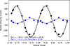 |
Fig. 3. Radial velocities of the gainer and donor star with their respective errors, using the lines 6562.8 Å for gainer and 6677.9 Å for donor. |
Radial velocities of the gainer and donor star.
To analyze each stellar component independently, we used an iterative spectral disentangling method developed by Gonzalez & Levato (2006). The method consists of the following: an initial set of radial velocities is assumed for each star (see Table 3). Using these velocities, the observed spectra are shifted to their individual rest frames and then combined. This combination generates a template that represents the flux contribution of a single star, although still slightly contaminated by the light of its companion. This process is repeated for the other star, thus generating the first spectral templates for each stellar component. These first templates are subtracted from each original spectrum to remove the individual contribution of each star. In the next iteration, the previous steps are repeated, generating new templates and performing the subtractions successively until convergence is reached and a clean average spectrum is obtained for both components. However, it is important to note that the disentangling method will not allow us to separate the contribution of the accreting star from that of a possible accretion disk, as there are no models available for the spectral lines of accretion disks.
2.4. Determination of stellar parameters by spectral fitting
In this study, the determination of the stellar parameters of each component was carried out by fitting synthetic spectra to previously unraveled observed spectra. To generate these synthetic spectra, we used the well known Spectrum5 code (Gray et al. 2001; Gray & Corbally 1994) which is based on stellar atmosphere models provided by ATLAS96 (Castelli & Kurucz 2003) is a recognized program in the field of astrophysics for spectral synthesis and analysis. It is used for generating synthetic spectra based on a range of stellar atmospheric parameters, including effective temperature (Teff), surface gravity (log g), and chemical composition. The incorporation of atomic and molecular data gives spectrum the ability to model the physical processes that allow the characteristics of stellar spectra to be recreated. This allows us to compare synthetic and observed spectra, thereby aiding in the determination of key stellar parameters such as temperature, metallicity, and rotational velocity. The versatility and adaptability of spectrum makes it a useful tool for probing chemical abundances and properties of astronomical objects in a spectral type range from B to M.
Therefore, a grid was constructed for the donor star with different free parameters, such as the (Teff), the (log g), the macroturbulence velocity (vmac), the microturbulence velocity (vmic), and the rotational velocity (v sin i), and even the veiling factor (η). This last parameter corresponds to a proportionality constant between the theoretical and observed spectra due to the light contribution from its companion, which has veiled the absorption lines. All spectra were constructed using a metallicity index similar to that of the Sun (M/H = 0.0) and a fixed mixing length parameter l/H = 1.25 by default. A chi squared optimization algorithm was implemented, which consists of minimizing the deviation between the normalized theoretical spectrum and the observed average spectrum of the donor. The theoretical model was produced by varying the aforementioned parameters as follows: the Teff varied from 3500 ≤ Td ≤ 10 000 K and 10 000 ≤ Td ≤ 30 000 K for the gainer, with a step of 250 K; the log g varied from 0.0 ≤ log g ≤ 5.0 dex, with a step of 0.5 dex; the macroturbulence velocity varied from 0 ≤ vmac ≤ 10 km s−1, with steps of 1 km s−1; while the microturbulence velocity took values of 0.0 and 2.0 km s−1, the rotational velocity varied from 10 ≤ v sin i ≤ 150 km s−1, with steps of 10 km s−1, and the veiling factor 0.0 ≤ η 5400 − 5700 Å ≤ 1.0, with steps of 0.1. The implemented method successfully converged to a minimum.
The synthetic spectrum that obtained the lowest chi square value χ2 = 0.49 relative to the donor spectrum was the one at 8750 ± 125 K, log g = 3.5 ± 0.25 dex and v sin i = 40 ± 5 km s−1. In the case of the gainer, several synthetic spectra achieved similar chi square values, so further checking is required. Figs. 4 and 6 show the disentangled spectra of the donor and gainer, along with the synthetic spectra that best achieved a fit.
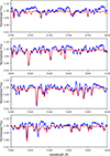 |
Fig. 4. Comparison of synthetic spectra (red line) with the Donor disentangled spectrum (blue line). The windows show portions of the spectrum from 4700 Å to 5400 Å. |
While the temperature of the donor star was effectively determined by fitting synthetic spectra generated with spectrum to its observed spectrum, minimizing the chi squared, the presence of an accretion disk around the accreting star complicates this direct approach. Therefore, to estimate the temperature of the accretor, spectral lines characteristic of B type stars were explored. The ratio between the equivalent widths of these lines could provide a valuable indication of the central star’s temperature, minimizing the influence of the disk. Each calibrated equivalent width relationship provides a measure of the stellar temperature. To identify Teff indicators, we conducted an exploratory survey across synthetic spectra generated by the spectrum. Our criteria for line selection required proximity for consistent continuum levels in observed spectra and distinct temperature dependent variations in line depths. From our analysis of lines between 4580 and 7590 Å in previously used synthetic spectra, only a pair of lines at S II 5640.32 Å and Cr II 5678.42 Å met these criteria (Fig. 5), which are located beyond telluric absorption lines.
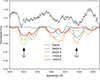 |
Fig. 5. Comparison of lines S II 5640.32 Å and Cr II 5678.42 Å in the synthetic spectra generated with Spectrum. The variation in the depth of each line with changes in temperature can be seen in the synthetic spectra. |
We applied the χ2 test to assess the equivalent width ratios from both synthetic and untangled spectra. Fig. 7 presents our adjustment of the values of χ2 with the temperature, where a comparison is made between observed EW ratios and theoretical EW ratios. This statistic indicates the degree of alignment of the data with the regression line, with values close to 1 denoting a strong correlation. It is important to note that line depths can be influenced by the star’s rotational velocity. To adapt this to the gainer, different speeds were tested in the synthetic spectra between 100 km s−1 and 250 km s−1, with 200 km s−1 being the one that gave the best fit. This analysis aimed to determine the temperature of the gainer by comparing the equivalent width ratio between its spectrum and the synthetic spectra. As can be seen in Fig. 7, the lowest value of χ2 was found in the range of 20 000–22 000 K, for log g = 3.0 ± 0.2 being the value with the lowest χ2, where a log g was varied between 2.5 and 4.0.
Using the untangled spectra, we deduced the probable spectral types for each component. The gainer star’s spectral characteristics align with a B2 or B3 classification, while the donor’s features suggest a A3 type. In the disentangled spectrum of the gainer (Fig. 6), emission wings are observed on either side of the main absorption lines, a feature that has also been reported in other DPV systems. Several studies have suggested that these wings could originate from circumstellar material associated with mass flows or bipolar winds. In particular, Mennickent et al. (2012b) proposed the existence of a cyclic bipolar wind in V393 Scorpii, originating from the interaction between the mass transfer stream and the accretion disk, thereby generating extended structures that produce photon scattering and broad emission wings in Balmer lines such as Hα and Hβ. Similarly, Rosales et al. (2023) observed line profiles with emission shoulders in V4142 Sgr, which they interpreted as evidence of an extended atmosphere around the gainer’s accretion disk, responsible for the formation of the wings. Additionally, Mennickent et al. (2010) and Mennickent et al. (2016b) highlighted that disk structures in DPVs, rather than being thin Keplerian disks, present irregular geometries and extended flows, all of these could be possible explanations for the wings detected in the disentangled spectra of V1001 Cen.
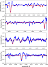 |
Fig. 6. Comparison of synthetic spectra (red line) with the Gainer disentangled spectrum (blue line). The windows show portions of the spectrum from 4900 Å to 6750 Å. |
2.5. Light curve synthesis model
Djurašević (1992b) proposed a light curve synthesis model for W Ser type binaries. In these binary systems, which are in a phase of high matter exchange between the components, a gaseous disk usually forms around the primary star. The Roche model is used to approximate the maximum size of these star systems, taking into account the effect of asynchronous rotation. Djurašević (1992b) applies the inverse problem method to estimate the fundamental orbital and physical parameters of the binary system. This technique involves constructing a model that simulates the system’s light curve behavior. By comparing the observed light curves with those predicted by the model, the parameters are iteratively adjusted to achieve the best fit. Certain parameters-such as the temperature of the gainer and the mass ratio-are held fixed, using values derived in earlier sections. Notably, the model does not incorporate the radial velocity data previously computed. The fitting procedure typically explores a range of values for key parameters, including mass, radius, and temperature. In particular, the radius of the accretion disk is estimated relative to the Roche lobe radius. For a detailed explanation of the methodology used to determine these physical parameters, refer to Djurašević (1992b, 1996). Djurašević (1996) modified the model to include a white dwarf companion, allowing it to be applied to another group of binary systems.
Thus, based on the light curve synthesis model mentioned, we calculate the best fit, the O-C residuals, along with the individual flux contributions of the donor, gainer, and disk of V1001 Cen, and include the view of the optimal model at orbital phases 0.05, 0.20, 0.50, and 0.80. From the residuals, we notice a scatter around ΔV ∼ 0.92 (mag) without dependencies related to orbital or long cycle phases. The best fitting model contains an optically and geometrically thick accretion disk surrounding a nonsynchronous gainer star with the presence of a bright and hot spot (see Fig. 8, Table 4).
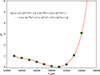 |
Fig. 7. Adjustment of a function of the values of χ2 from the comparison of theoretical and observed EW ratios vs. temperature. |
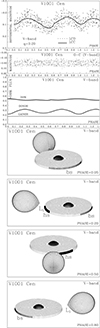 |
Fig. 8. Observed (LCO) and synthetic (LCC) light curves of the system V1001 Cen obtained by analyzing ASAS V band photometric observations and final O-C residuals between the observed and optimum synthetic light curves; fluxes of donor, gainer and of the accretion disk, normalized to the donor flux at phase 0.25; the views of the optimal model at orbital phases 0.05, 0.20, 0.50 and 0.80, obtained with parameters estimated by the light curve analysis. |
In this study, the gainer star is assumed to be surrounded by an accretion disk, without considering other potential sources of emission, such as jets, stellar winds, or gas streams. However, our model allows us to include azimuthally dependent variations in the emissivity of the disk by introducing two emitting spots in the disk (a bright spot and a hot spot). Bisikalo et al. (1998, 1999, 2003) studied the hydrodynamic simulations of mass transfer in close binaries, suggesting the possibility of forming hot and bright spots in the accretion disk. These spots may represent shock regions characterized by higher density and temperature than the surrounding medium. Although this simplification has certain limitations and despite excluding possible external contributions, previous investigations in Algol systems with disks suggest that this model adequately represents the main sources of emission in the light continuum.
Our findings indicate that the best fitting model of V1001 Cen contains an optically and geometrically thick disk surrounding the hottest and most massive gainer star (Table 4). The radius of the disk, Rd = 13.2 ± 0.1 R⊙, It is approximately 5 times larger than that of the central star (Rg = 2.68 ± 0.1 R⊙). The disk has a relatively flat shape, with a central thickness dc = 1.32 ± 0.1 R⊙ and an edge thickness of 1.25 ± 0.1 R⊙. The temperature of the disk increases from Td = 7415 ± 500 K at its edge to Tg = 18 310 ± 500 K at the inner radius, where it is in physical and thermal contact with the gainer star. The disk temperature is the same as the gainer at its inner edge and decreases with a radial profile described by an exponent, aT.
Results of the analysis of V1001 Cen ASAS V band light curves.
 (5)
(5)
where Tg and Rg denote the temperature and radius of the donor star, respectively. The constraint aT < 0 ensures that the temperature decreases radially outward from the star.
In the best model, we observe a hot spot with an angular radius of 21.° 6 ± 1.° 2, located at longitude λhs = 326.° 9 ± 3.° 0, approximately between the components of the system. This is where the gas current falls on the disk (Lubow & Shu 1975). The hotspot temperature is 9787 ± 500 K. Although including the hotspot region in the model improves the fit, it does not fully represent the asymmetry in the light curve. Hence, an additional bright spot is introduced, larger than the hotspot and located at λbs = 172.° 7 ± 8.° 0 on the disk’s edge, leading to a much better fit. This bright spot has Tbs = 10 232 ± 500 K and an angular radius of 49.° 5 ± 1.° 3. The lambda angles are measured from a line that joins the center of the donor with the center of the gainer, in the opposite direction to the orbital motion, and the theta angle measures the angular extension of the spots. To learn more about how the size, position, and temperature of the spots are calculated, we recommend reading the work of Djurašević (1992a). Due to the inclination of the system (68.° 3 ± 0.° 3), it was necessary to assume that it is the disk that is hidden during the eclipse, which can lead to the exposed errors being less than the possible real errors.
The results of the analysis were obtained from solving the inverse problem for the Roche model with an large accretion disk partially obscuring the more massive (hotter) gainer in critical nonsynchronous rotation regime.
Fixed parameters: q = ℳc/ℳh = 0.20 – mass ratio of the components, Tc = 8750 K – temperature of the less massive (cooler) donor, Fc = 1.0 – filling factor for the critical Roche lobe of the donor, fh = 20.0; fc = 1.00 – nonsynchronous rotation coefficients of the gainer and donor respectively, βh = 0.25; βc = 0.25 – gravity darkening coefficients of the gainer and donor, Ah = 1.0; Ac = 1.0 – albedo coefficients of the gainer and donor.
Quantities: n – number of observations, Σ(O − C)2 – final sum of squares of residuals between observed (LCO) and synthetic (LCC) light curves, σrms root mean square of the residuals, q = ℳc/ℳh – mass ratio of the components, i – orbit inclination (in arc degrees), Fd = Rd/Ryc – disk dimension factor (ratio of the disk radius to the critical Roche lobe radius along y axis), Td – disk edge temperature, de, dc – disk thicknesses (at the edge and at the center of the disk, respectively) in the units of the distance between the components, aT – disk temperature distribution coefficient, Fh = Rh/Rzc = 1.0 – filling factor for the critical nonsynchronous lobe of the hotter, more massive gainer (ratio of the stellar polar radius to the critical nonsynchronous lobe radius along z axis for a star in critical rotation regime), Th – temperature of the more massive (hotter) gainer, Ahs, bs = Ths, bs/Td – hot and bright spots’ temperature coefficients, θhs, bs and λhs, bs – spots’ angular dimensions and longitudes (in arc degrees),θrad – angle between the line perpendicular to the local disk edge surface and the direction of the hot spot maximum radiation, Ωh, c – dimensionless surface potentials of the hotter gainer and cooler donor, ℳh, c[M⊙], ℛh, c[R⊙] – stellar masses and mean radii of stars in solar units, log gh, c – logarithm (base 10) of the system components effective gravity,  – absolute stellar bolometric magnitudes, aorb [R⊙], ℛd[R⊙], de[R⊙], dc[R⊙] – orbital semi major axis, disk radius and disk thicknesses at its edge and center, respectively, given in the solar radius units.
2.6. TESS photometric data and comparison with ASAS
The TESS satellite (Transiting Exoplanet Survey Satellite) performs a nearly all sky photometric survey in the near optical band, observing most of the sky in sectors of approximately27–28 days, providing a temporal coverage of about one month for the V1001 Cen system. TESS photometry is of very high precision: according to Ricker et al. (2015), TESS is expected to achieve a photometric precision of 60 ppm on hourly timescales for bright stars. In fact, thousands of high quality light curves for eclipsing binary systems have been published thanks to TESS observations (Prša et al. 2022; Ricker et al. 2015).
In contrast, the ASAS instrumentation provides photometry in V and I bands to a relative accuracy of 0.01–0.02 mag. for stars brighter than 10th magnitude (Pojmański 2001). Its cadence is one or two points per night, which allows one to trace light curves of long period systems, albeit with a significantly higher dispersion than TESS. Due to its limited temporal coverage (∼27 days), TESS data do not allow for the derivation of long term parameters such as modulation cycles or long periods.
To assess the compatibility between both datasets, we fit a Fourier series to the ASAS light curve, as shown in Figure 9. This fit curve (red line) was then compared with the TESS data (blue points) for the same system. We find that the ASAS based fit reproduces the TESS light curve with very good agreement; the differences are minimal and limited primarily to slight variations in the depth of the secondary eclipse. In other words, the light curve models fit to ASAS data reproduce the main features also observed by TESS.
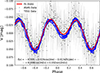 |
Fig. 9. Light curve of V1001 Cen derived from ASAS data (black points) and TESS data (blue points). The red line corresponds to a Fourier series fit to the ASAS data. A good agreement is observed between the fit function and the TESS photometry, indicating consistency between both datasets. |
Therefore, it is not strictly necessary to recalibrate a new light curve synthesis model based solely on the TESS data. The photometric model derived from ASAS data is fully compatible with TESS photometry within the expected uncertainty, indicating that the fundamental eclipse properties (phase, shape, and duration) are preserved. Nevertheless, the higher photometric precision and continuous coverage of TESS could allow for refinement of some sensitive parameters, such as the depth of the secondary eclipse or the size of the accretion disk. However, these adjustments would not significantly affect the other physical parameters derived in the synthesis model discussed in Section 2.5.
Furthermore, using the TESS data, we plotted a periodogram using the Lomb Scargle method from the gatspy python library to investigate the possible presence of other significant periodicities in the TESS data, as shown in Figure 10. The resulting periodogram shows that the dominant periodicity corresponds to the known orbital period, previously derived from the ASAS dataset. No additional significant periods were detected within the time span covered by TESS. This result supports the consistency between the ASAS and TESS datasets, reinforcing the conclusion that the ASAS photometry captures the essential periodic features of the system, also observed in the high precision TESS data.
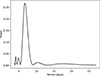 |
Fig. 10. Periodogram of the TESS data for V1001 Cen. The periodogram reveals a dominant period consistent with the previously determined orbital period from ASAS data. No additional significant periodic signals are detected. |
2.7. Discussion on the spectral distribution of energy and the circumstellar disk
To construct the spectral energy distribution (SED) of V1001 Cen, we compiled the available photometric fluxes for this system. We extracted this information from the Vizier photometric viewer. We selected theoretical models of individual stars using the Virtual Observatory SED Analyzer (VOSA; Bayo et al. 2008) to perform a fit to the SED. This fit allowed us to determine the albedo of the system’s accretion disk. For this process, we kept the distances provided by Gaia DR37 fixed. Our models were centered using parameters from Subsection 2.5, specifically: a cool star with an effective temperature (Teff, c) of 8750 K and a surface gravity (log gc) of 3 dex, an Teff for the hot star (Th) of 18 000 K, and a (log gh) of 4.0 dex. Furthermore, we considered an interstellar reddening value of E(B − V) = 0.6351 ± 0.0292 (mag) (Schlafly & Finkbeiner 2011). The model that best fits our data is the one that minimizes the reduced χ2, considering the composite flux described by the following equation (Fitzpatrick & Massa 2005):
![Mathematical equation: $$ \begin{aligned} f_{\lambda }=f_{\lambda ,0} 10^{-0.4E(B-V)[k(\lambda -V)+R(V)]}. \end{aligned} $$](/articles/aa/full_html/2025/11/aa53975-25/aa53975-25-eq9.gif) (6)
(6)
In this equation, E(B − V) represents the color excess, which quantifies how much the star’s light has been reddened due to interstellar dust. The term k(λ − V)≡E(λ − V)/E(B − V) is the normalized extinction curve, which describes how extinction varies as a function of wavelength (λ) relative to the V band. On the other hand, R(V)≡A(λ)/E(B − V) is the ratio between the total extinction (A(λ)) and the reddening in the V band. The term fλ, 0 corresponds to the sum of the intrinsic surface fluxes of both stars at wavelength λ, before being affected by interstellar reddening, and is calculated as:
![Mathematical equation: $$ \begin{aligned} f_{\lambda ,0}= \left(\frac{R_{\rm c}}{d} \right)^{2} \left[\left(\frac{R_{\rm h}}{R_{\rm c}} \right)^{2}f_{\rm h,\lambda }+f_{\rm c,\lambda } \right] + \left(\frac{R_{\rm disk}}{d}\right)^{2}f_{\rm disk,\lambda }, \end{aligned} $$](/articles/aa/full_html/2025/11/aa53975-25/aa53975-25-eq10.gif) (7)
(7)
where fh, λ and fc, λ represent the fluxes of the hotter and cooler star, respectively, and fdisk, λ the flux corresponding to the accretion disk. The normalized extinction curve k(λ − V) was calculated using the prescriptions described in Martin & Whittet (1990) and Cardelli et al. (1989).
In essence, we analyzed the light reaching us from V1001 Cen in different colors (photometric fluxes) and compared it with the light predicted by theoretical models of two stars. To make this comparison accurately, we took into account the distance to the system, obtained from the high precision data of Gaia DR3. Furthermore, we corrected for the effects of interstellar dust, which alters the colors of starlight. The equation used to model the total flux considers the contribution of both stars, taking into account their relative sizes (Rc and Rh relative to the distance d) and their intrinsic fluxes at each wavelength. The best model is the one that, after applying the correction for interstellar reddening, most faithfully reproduces the observed fluxes, which is quantified by minimizing the reduced χ2. This process allowed us to obtain valuable information about the system’s properties, including the albedo of its accretion disk.
To define this contribution, we used expression (5.9) from Frank et al. (2002):
 (8)
(8)
where
 (9)
(9)
Replacing this expression, we obtain
 (10)
(10)
which shows that the disk flux is directly related to  , with T⋆ being the temperature of the accretor. This allowed us to model the additional flux contribution in the theoretical equation of the spectral flux as a percentage of the accretor’s flux. This percentage factor (1 − β)cos φ, which represents the disk albedo, is parameterized as part of Equation (7). From the disk thickness data extracted from Table 4, we can estimate the factor cos φ ≈ 1, whereby our albedo factor mainly depends on (1 − β). For our minimization of (1 − β), this factor was a free parameter that varied in the range of 0 to 1. And for our case, the best fit is (1 − β) = 0.34. Fig. 11 shows the best χ2 minimization found to represent the SED of V1001 Cen.
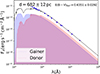 |
Fig. 11. Spectral energy distribution and the best χ2 minimization. |
For the value of the fractional radius of the gaining object, R1/a = 0.1, it has been found that there is enough space for the formation of an accretion disk, considering the mass ratio of the system. In this case, the star acting as a mass receiver is smaller than the circularization radius, where a particle released from the inner Lagrangian point can conserve its angular momentum Lubow & Shu (1975). This low fractional radius is attributed to the separation and orbital period of the system, which is consistent with the existence of an accretion disk inferred from the light curve model. Furthermore, the calculated value is similar to that obtained in long period systems such as V495 Cen (Rosales et al. 2019, 2021). Note that the vertical height of the disk near the receiving object is approximately half the radius of the receiving object, causing partial occultation of the star.
Under hydrostatic equilibrium conditions, the vertical height, H, of a disk of radius R, in chapter 3 of the book (Kolb 2010) he defines it as:
![Mathematical equation: $$ \begin{aligned} H = 10^{4}\sqrt{\frac{T}{10^{4}\, K}} \sqrt{\frac{R^{3}}{GM_{1}}} \quad [\mathrm{ms}^{-1}]. \end{aligned} $$](/articles/aa/full_html/2025/11/aa53975-25/aa53975-25-eq15.gif) (11)
(11)
The above equation predicts that for V1001 Cen, a disk in hydrodynamic equilibrium would have a relative thickness H/R of 0.10 and H = 9.47 × 10⁸ m, indicating a thin disk. The data in Table 4 confirm this prediction: the disk thickness at the edge (de/R = 0.09) is close to the theoretical value, suggesting a low thermal pressure disk in hydrodynamic equilibrium. However, in the immediate vicinity of the star, the disk widens significantly (dc/R = 0.49), covering almost half of the stellar radius. This fivefold increase in thickness cannot be explained by a temperature rise alone, as the thermal conditions of the disk do not justify such a dramatic expansion. Instead, this behavior can be attributed to the presence of turbulent motions within the disk, which increase the velocities beyond those expected for a Keplerian disk in thermal equilibrium. These turbulent motions enhance the vertical support of the disk, leading to the observed increase in the H/R ratio near the star.
Theoretically, the disk could be stable until reaching the tidal radius (Paczynski 1977; Warner 2003), which defines the last nonintersecting orbit:
 (12)
(12)
We have compiled the outer disk radii and the primary star radii for the DPV systems from Table 12 of the Mennickent et al. (2016a) paper. These radii, relative to the binary separation, are plotted in Fig. 12. The plot R1/a versus q has previously been used to differentiate between Algol systems with and without disks (Plavec 1989; Vanbeveren 2013), and the observation of V1001 Cen is highlighted in Fig. 12. Based on those authors, three theoretical radii that are widely used to understand disk dynamics and mass transfer in binary systems are included in this analysis.
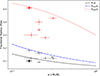 |
Fig. 12. Relative radius for the Gainer R1/a (black dot) and disk (Rd/a (red dot) of V1001 Cen, the gray dots are other DPVs extracted from Table 12 of Mennickent et al. (2016a), and the pink dots represent their disks. Below the circularization radius shown by the dashed black line a disk should form and below the dashed blue line a disk could form. The tidal radius indicates the maximum possible extent of the disk. |
The first radius is the critical radius, defined by Lubow & Shu (1975) and approximated by Hessman & Hopp (1990):
 (13)
(13)
This critical radius represents the maximum limit for the size of the primary star that allows the formation of an accretion disk. At this point, the specific angular momentum of a particle orbiting the critical radius is equal to that of a particle released from the inner Lagrangian point, L1. This implies that the critical radius marks the maximum extent of a ring of matter that can form due to the Roche lobe overflow just before viscosity begins to expand the material into a disk. If the radius of the primary star exceeds this limit (R1 > rc), the system is classified as an impact system, where the gas flow hits the star directly, significantly reducing the chances of formation of accretion disks.
In real systems, because of the finite size of the gas flow, it is still possible for some outer orbits of the gas stream to escape the direct impact. This phenomenon generates a maximum effective radius, rmax, which is slightly larger than rc and depends on the mass ratio q of the system Lubow & Shu (1975). This limit is also included in Fig. 12 to provide a more complete representation.
The second key radius is the tidal radius, derived by Paczynski (1977) and Warner (2003):
 (14)
(14)
This radius defines the last nonintersecting orbit of the accretion disk. It is assumed that, as the disk grows, it begins to experience strong shear forces as a result of gravitational and viscous interactions. Therefore, the tidal radius sets an upper limit for the size of the disk, beyond which the disk material is significantly perturbed or redistributed.
The combination of these three theoretical radii (the critical radius, the maximum radius, and the tidal radius) provides a comprehensive view of the dynamical configurations possible in binary systems. These limits help characterize the mass transfer and accretion disk structure, key elements in the evolution of binary stellar systems.
For the case of the V1001 Cen gainer with a value of R1/a slightly lower than rc as seen in Fig. 12, it would indicate that the mass flow does not reach the star and collides with itself at a larger radius. The radial motion dissipates and the resulting ring of material spreads viscously to form an accretion disk. It should be noted that the disk has an extension comparable to the tidal radius, its maximum possible boundary.
The gainer star has a mass of 4.25 solar masses and a temperature of 18 310 K. This temperature is unusually high for a star with this mass. However, it is possible that the accreted material favors a particularly efficient hydrogen burning in the core, which would allow higher temperatures to be reached. Another factor to consider is that the gainer star’s metallicity could be relatively low, which would cause its atmosphere to be less opaque, allowing for greater energy emission. This could give rise to a pseudo photosphere that contributes to the observed temperature increase. Another possibility for the excess temperature in the gain star may be due to the presence of a pseudophotosphere around it. This phenomenon has already been observed in the DPV AU Monocerotis studied by Armeni & Shore (2022), in their work they studied different spectral lines in the ultraviolet and optical range, the spectrum of the hot star suggests that some optical absorption lines, such as the Balmer and Mg II 4481 Å lines, are not completely photospheric, but have a significant contribution from circumstellar material, particularly in the weak states of the long cycle. UV resonance lines (such as Mg II, Al II, and Si II) come mainly from the accretion disk and not from the photosphere of the star. This confirms the existence of a stratified environment around the gainer. Star B shows rapid rotation and features consistent with the presence of an optically thick boundary layer (pseudo photosphere). This suggests that the visible surface of AU Monocerotis is affected by accretion disk material, which alters the spectrum and temperature derived from spectral observations, the same could happen in V1001 Cen.
3. Evolutionary modeling of V1001 Cen with MESA
MESA (Modules for experiments in stellar astrophysics) is an open source stellar evolution code used in astrophysical research developed by Paxton et al. (2015). This software enables the study of a variety of stellar phenomena, ranging from the evolution of individual stars to binary systems and stellar explosions. MESA allows researchers to accurately model stellar evolution, including processes such as nucleosynthesis, stellar pulsations, and the evolution of massive stars toward final stages such as supernovae or neutron stars.
Paxton et al. (2015) introduced a new module in MESA called MESAbinary, which allows for the simultaneous evolution of pairs of stars that rotate differentially, greatly enhancing the model’s ability to simulate binary evolution. The inclusion of this module in MESA expands the possibilities for exploration in the field of astrophysics, allowing researchers to model binary systems with greater precision and their complex interactions.
To learn more about the features and functionalities of MESA, please refer to the original articles Paxton et al. (2019, 2018, 2015, 2010), Jermyn et al. (2023) and their cited references.
For our evolutionary models of binary systems, we use the MESA code version 22.11.1. Given that V1001 Cen is classified as a DPV system, we chose to use a formulation of the MESA code previously developed by Rosales et al. (2019) to study the DPV V495 Cen, and in his most recent study of the V4142 Sgr (Rosales et al. 2024). In his most recent model, Rosales develops an intermediate mass binary system where the gainer star is constrained by the Eddington accretion rate, preventing high rate accretion. Eventually, the donor star fills the Roche lobe, triggering a significant mass transfer and the formation of an accretion disk. This approach aims to replicate the physical conditions under which these stellar systems are believed to exist.
Evolutive stages from the donor star for DPV V1001 Cen.
The formalism proposed by Rosales et al. (2024, 2019) introduces certain initial parameters that are modified compared to the default parameters used by MESA. Here, we succinctly outline these parameter adjustments. Our initialization of our MESA model incorporates a metallicity value of Z = 0.02, this metallicity value was used because V1001 Cen is located within the disk of our galaxy, and Z = 0.02 is usually the classical reference value to represent stars with solar metallicity. In turn, a initial surface rotation velocity of 26 km s−1 for the donor star, aimed at activating the magnetic dynamo mechanism defined by the Spruit Tayler paradigm, with a mixing diffusivity value of Spruit Tayler DST = 0.1.
Our models employ the mass transfer scheme of Kolb & Ritter (1990). In seeking a conservative approach, we explored a range of values for the mass loss fractions through winds. For the fraction of mass lost from the vicinity of the donor as a fast wind (α), we varied the values between 0.0005 ≤ α ≤ 0.5 with increments of 0.001. Similarly, for the fraction of mass lost from the vicinity of the accretor as a fast wind (β), we explored the range 0.0001 ≤ β ≤ 0.1 with a step of 0.0001. Following this exploration, we determined that the values of α = 5 × 10⁻³ and β = 1 × 10⁻⁴ were the most suitable for maintaining a conservative system in our simulations, thereby minimizing mass loss during the transfer events and favoring the reproduction of a conservative system. Additionally, we incorporate Reimers prescription for mass loss during the RGB phase, utilizing the scale factors of wc, R = 0.8 and Blocker’s definition during the AGB phases with wc, B = 1.0. Furthermore, the loss attributed to a hot wind employs a Dutch type scheme with wh, D = 0.8.
For convection, we adopt the theory proposed by Henyey et al. (1965). Our models include the usage of Rosseland radiative opacity values for high temperatures, while the OPAL opacity tables Iglesias & Rogers (1993, 1996), particularly Type 1, are integrated for temperatures exceeding 104 K. To extend capabilities, we enable the Type 2 OPAL tables essential for helium burn and beyond.
Overshooting in MESA depends on the classification of the convective zone, with variability at the top and bottom of the zone. The parameters for exponential diffusive overshoot are elucidated by Herwig (2000) in his paper “The Evolution of Convective Overshoot AGB Stars”.
A critical aspect of overshooting control involves aligning the convective zone and the convection limit criteria. This necessitates defining the “overshoot_zone_type,” “overshoot_zone_loc,” and “overshoot_bdy_loc” for each convective boundary, along with relevant overshoot parameter values. In the Rosales model, the types of overshoot zone are specified for H, He, and Z, accompanied by the location of the overshoot zone for the shell and core, and the location of the overshoot boundary for both the upper and lower limits. The transition from convective mixing to overshooting occurs at a distance of (f0 ⋅ Hp) within the convection zone from the estimated position, with Hp signifying the height of the pressure scale at that location.
In MESA, overshooting is achieved by extrapolating the diffusion mixing coefficient beyond the edge of the convection zone. However, precisely at the edge of the zone, the mixing coefficient drops to zero, which is suboptimal. To address this concern, the parameter f0 designates the distance from the edge where the overshooting begins. In addition, the code accommodates the specification of how far back into the zone the overshooting should extend, denoted in terms of scale height. Essentially, the overshooting starts at a location determined by f0, some distance before the edge of the actual convection zone. For this study, ‘f0’ was established at 0.0005, and ‘f’ was established at 0.001. Readers interested in a more comprehensive explanation of the MESA formalism used in this study are encouraged to review the work of Rosales et al. (2024, 2019).
We conducted tests on initial masses ranging from 1.0 to 5.0 solar masses, and mass ratios (q) ranging from 0.9 to 0.3. The initial periods ranged from 1.0 to 3.0 days. The initial eccentricities were set to zero. All models were initiated from the main sequence and stopped when the donor star depleted its core helium ( ) or until the end of the evolutionary time step.
Following Mennickent et al. (2012b), a multiparametric fit was performed with the synthetic stellar parameters (Si, j, k) and observed (Ok), including mass, temperature, luminosity, radii and orbital period. The parameters were derived from MESA models, where i (ranging from one to n) indicates the model number, j (ranging from one to m) represents the step number within each model, and k (ranging from one to nine) denotes the stellar or orbital parameter.
![Mathematical equation: $$ \begin{aligned} \chi _{i,j}^{2}\equiv (1/N)\sum _{k}\omega _{k}[S_{i,j,k}-O_{k}/O_{k}]^{2}, \end{aligned} $$](/articles/aa/full_html/2025/11/aa53975-25/aa53975-25-eq20.gif) (15)
(15)
where N is the number of observations (9) and ωk is the statistical weight of the parameter Ok, calculated as
 (16)
(16)
The error associated with the observable Ok is represented by the variable ϵ(Ok). From the light curve synthesis study, we observed that the gainer has an accretion disk that dominates its luminosity. This causes the observed brightness of the gainer to be much higher than predicted by the MESA models. Therefore, for the parametric adjustment, we consider the observed physical values of the donor and the gainer.
Our model aims to identify the best fit, and we calculate the value of χ2 for each model. In the case of conservative models (without mass loss during the transfer phase) with the lowest χ2 = 0.29, the best fit suggests that the initial parameters of the binary system are an orbital period of Pi, o = 2.1 days, donor star mass of Md, i = 4.4 M⊙, and gainer star mass of Mg, i = 1.4 M⊙. The system is found in the rapid mass transfer phase, in an almost conservative mass transfer stage with Ṁ = 1.13 × 10⁻⁷ M⊙ yr−1, and an age of 190 Myr.
The HR diagram for the conservative model is shown in Fig. 13. The evolution of stars in the V1001 Cen system begins in the initial main sequence (ZAMS), with hydrogen burning, marked as point A. During this phase, the donor star maintains a mass of 4.399 M⊙ and a radius of 2.523 R⊙ while its core burns hydrogen and produces helium. This initial process allows the star to retain its stellar parameters without significant changes until it reaches an age of 132.359 Myr, at which point the mass transfer process (point C) begins. In this phase, the donor star begins to expand and transfer mass to its companion, causing a gradual decrease in its central hydrogen.
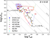 |
Fig. 13. Evolutionary model with conservative mass transfer for V1001 Cen. Initial orbital period of 2.1 days, initial masses of 4.4 and 1.4 M⊙. The dashed lines represent the evolutionary paths of single stars with initial masses equal to those of the binary model, the other points represent other known DPVs. |
When the central hydrogen of the star reaches low values (point D), its mass is reduced to 4.064 M⊙. At this stage, the mass transfer process intensifies, allowing the system to reach a mass reversal state (point U1) at an age of 132 400 Myr, when the donor mass drops to 3.863 M⊙. Consequently, the system undergoes a rapid evolution in luminosity and temperature. Subsequently, the donor star reaches the minimum value of its Roche lobe (point E) at 132.552 Myr, with a mass of 1.467 M⊙. This marks the beginning of a further expansion phase, which finally culminates at the end of the first mass transfer phase (point F), at 147 785 Myr.
Upon reaching 184 Myr (point G), the donor star enters a second phase of mass transfer, and its mass decreases even further, reaching a value of 1.157 M⊙, while its radius contracts to 3.777 R⊙. Finally, in the current stage (point X2) at 190.675 Myr, the donor star maintains a mass of 0.806 M⊙ and an extended radius of 6.563 R⊙, evidencing the advanced structural change in its core and envelope. The system reaches the end of its second mass transfer phase (H point) at 192.982 Myr, with a minimum mass of 0.482 M⊙ and an expanded radius at12.848 R⊙.
The adjustment of the radius, mass, and period of the V1001 Cen system is best represented by this model, allowing for a detailed analysis of these fundamental properties of the system (see Fig. 14 for period vs. mass, Fig. 15 for mass vs. radius and Fig. 16 for mass transfer vs. mass). Furthermore, the distribution of helium and hydrogen in the H–R diagram of V1001 Cen reflects how the transfer of material from the donor star rejuvenates the gainer star (see Fig. 17).
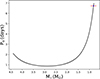 |
Fig. 14. Evolution of the orbital period as a function of the mass of the donor star of V1001 Cen. |
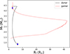 |
Fig. 15. Schematic behavior of radius and mass for both stars. The gainer star decreases its radius, while the donor star expands to fill the Roche lobe. |
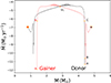 |
Fig. 16. Theoretical variation in mass transfer until reaching the helium depletion for initial masses of 4.4 and 1.4 M⊙. |
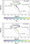 |
Fig. 17. Hertzsprung Russel (H–R) diagrams illustrate the evolution of binary stars. The color bar indicates the proportion of hydrogen and helium in the core of each star. |
The internal structure and evolution of each star in the V1001 Cen system for the conservative model can be visualized using the Kippenhahn diagrams (see Fig. 18). The upper diagram represents the evolution of the donor star with an initial mass of Md, i = 4.4 M⊙, while the bottom one shows the evolution of the gainer star with an initial mass of Mg, i = 1.4 M⊙. Both models are limited to the point where the donor star reaches helium core depletion, with XHec < 0, 1. The x axis represents the star’s age in units of millions of years.
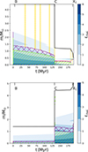 |
Fig. 18. Kippenhahn plots derived from the MESA model with conservative mass transfer for V1001 Cen. At the top we see graph donor star and below gainer star for a conservative model of initial mass of 4.4 and 1.4 M/M⊙ and initial orbital period of 2.1 days. In the graphical representation, the x axis displays the age since hydrogen ignition in units of million years (Myr), and the different stellar layers are identified by their mass proportions (M/M⊙). Each mixing process is illustrated with specific colors and patterns: convective mixing is represented in green with a hatching pattern, semi convective mixing in red, convective overshooting mixing with a crosshatched pattern in purple, and thermohaline mixing in yellow with a hatching pattern. The solid black line indicates the surface of each star, and the brown zones correspond to rotational mixing. |
The different layers are characterized by their M/M⊙ values, with convective mixing shown in dashed green, semiconvective mixing in red, overshooting mixing in dashed violet, thermohaline mixing in dashed yellow, and the continuous black line indicating the surface of each star.
In the field of astrophysics of binary star systems, specifically in DPVs, Equation (7) from the Schleicher & Mennickent (2017) study emerges as a fundamental pillar for understanding the relationship between the dynamo cycle and the rotation period in these systems. This equation is instrumental in unraveling the complex magnetic interactions inherent to DPVs.
The equation is expressed as follows:
![Mathematical equation: $$ \begin{aligned} P_{\text{cycle}} = \left( \frac{11.5 \, v_{\rm c} P_{\text{Kep}} R_{\odot }}{\epsilon _{\rm H} R_{2} [ \text{ kms}^{-1}\,\text{ yr}]} \right)^{-2\alpha } P_{\text{rot}}. \end{aligned} $$](/articles/aa/full_html/2025/11/aa53975-25/aa53975-25-eq22.gif) (17)
(17)
In this formula, Pcycle denotes the dynamo cycle period, vc represents the convective velocity, PKep is the Keplerian orbital period, ϵH a parameter that links the height of the pressure scale with the Roche radius, R2 the radius of the secondary star, and Prot the rotation period of the star. The factor α is interpreted as a power law index.
This model helps to understand how the dynamo cycle is intrinsically linked to the orbital period in DPV systems. The convective velocity vc and the radius of the secondary star are parameters extracted from fit MESA models, where vc is determined as the maximum value in the possible convective regions within the donor star modeled with MESA. The Kepler period PKep is calculated using expression 6 from Schleicher & Mennickent (2017).
To estimate the value of the dynamo number and therefore the coefficient α, we used the orbital and long periods obtained from photometry. These periods are inserted into Equation 15 to estimate α, whose value, according to Schleicher & Mennickent (2017), should oscillate between 0.33 and 0.83. Table 6 of the study presents the calculated values of the dynamo number and α for the best fit MESA model. In Table 6, the theoretical values of the short and long periods, estimated using the calculated dynamo number, are also included.
Values for the conditions of the long period for the V1001 Cen.
4. Conclusions
-
In this study, we conducted a comprehensive analysis of the V1001 Cen binary system, classified as a DPV. This system consists of a giant star with solar abundance and a temperature of 8750 K, and an early type B star with a temperature around of 20 000 ± 2000 K. Through a detailed spectroscopic study, we have determined a mass ratio of q = 0.151 ± 0.003, based on the observed radial velocities.
-
Our light curve model incorporates the effects of an optically thick accretion disk around the gainer star. We identified two bright regions on the disk, located at longitudes λ = 172° ±8 and 326° ±3. These regions exhibit temperatures between 32 and 38 percent higher than that of the disk’s outer edge. It is plausible that these bright spots correspond to shock regions generated during mass transfer, a phenomenon commonly observed in hydrodynamic simulations of interacting binary systems.
-
Regarding the evolutionary stage, V1001 Cen is a second phase of mass transfer. According to our conservative mass transfer model, the estimated age of the system is 190 million years, with a mass transfer rate of Ṁ = 1.13 × 10⁻⁷ M⊙ yr−1. We observe that the donor has depleted hydrogen in its core, while the gainer, although in the main sequence phase, shows signs of early evolution. The hydrogen enrichment in the gainer star leads to rejuvenation, repositioning it within the main sequence.
-
Our most suitable model for the conservative case suggests that V1001 Cen is a DPV resulting from the evolution and mass transfer of two stars with initial masses Mi, d = 4.4 M⊙ and Mi, g = 1.4 M⊙, and an initial orbital period of 2.1 days.
-
It was also possible to evaluate the presence of the second period, successfully reproducing it for V1001 Cen, for which it was found necessary to employ a dynamo number of D = 7884.74 and a power law index α = 0.71 (dimensionless) in the theoretical models. Additionally, the identification of two distinct stages in the evolutionary track of the system, such as the minimum value Roche lobe (E stage) and the current stage of the system (X2-stage), not only confirms stellar dynamo activity but also suggests the possibility of its onset in an early phase of evolution, possibly from the Roche lobe minimum. This finding provides a valuable perspective on the generation of magnetic fields and the modulation of activity in interacting binary systems such as V1001 Cen.
-
Finally, we evaluated the conditions necessary for the formation of a circumstellar disk around the gainer star. Our results indicate that the gainer star is within the range of parameters in which the formation of such structure is possible.
-
The analysis of the light curve modeling yielded an albedo for the accretion disk of (1 − β = 0.34). This value is fundamental to understanding how much light from the stellar surface is reflected by the disk, being a key parameter in the study of the interactions and heating processes within the V1001 Cen binary system.
Acknowledgments
P.A.C. acknowledges ANID project 21202285. R.E.M. and P.A.C. acknowledges BASAL (CATA) PFB-06/2007 and FONDECYT 1190621. J.A.R.G gratefully acknowledges support by the grant Vicerrectoría de Investigación y Desarrollo (VRID) Postdoctoral DICA N181/23 P.A.C. This research was partially funded by a scholarship during the first years of study at the Faculty of Physical and Mathematical Sciences of the University of Concepción (UdeC).
References
- Armeni, A., & Shore, S. 2022, A&A, 664, A103 [NASA ADS] [CrossRef] [EDP Sciences] [Google Scholar]
- Bayo, A., Rodrigo, C., Barrado Y Navascués, D., et al. 2008, A&A, 492, 277 [NASA ADS] [CrossRef] [EDP Sciences] [Google Scholar]
- Bisikalo, D., Boyarchuk, A., Chechetkin, V., Kuznetsov, O., & Molteni, D. 1998, MNRAS, 300, 39 [NASA ADS] [CrossRef] [Google Scholar]
- Bisikalo, D., Boyarchuk, A., Chechetkin, V., Kuznetsov, O., & Molteni, D. 1999, Astron. Rep., 43, 797 [Google Scholar]
- Bisikalo, D., Boyarchuk, A., Kaigorodov, P., & Kuznetsov, O. 2003, Astron. Rep., 47, 809 [NASA ADS] [CrossRef] [Google Scholar]
- Cardelli, J. A., Clayton, G. C., & Mathis, J. S. 1989, in Interstellar Dust, eds. L. J. Allamandola, & A. G. G. M. Tielens, IAU Symp., 135, 5 [Google Scholar]
- Castelli, F., & Kurucz, R. 2003, A&A, 210, A20 [NASA ADS] [Google Scholar]
- Djurašević, G. 1992a, Astrophys. Space Sci., 196, 267 [Google Scholar]
- Djurašević, G. 1992b, Astrophys. Space Sci., 197, 17 [Google Scholar]
- Djurašević, G. 1996, Astrophys. Space Sci., 240, 317 [Google Scholar]
- Eyer, L., & Blake, C. 2002, in Radial and Nonradial Pulsationsn as Probes of Stellar Physics, ASP Conf. Ser., 259, 160 [Google Scholar]
- Fitzpatrick, E. L., & Massa, D. 2005, AJ, 130, 1127 [NASA ADS] [CrossRef] [Google Scholar]
- Frank, J., King, A., & Raine, D. J. 2002, Accretion Power in Astrophysics, 3rd edn. [Google Scholar]
- García, G. R., Mennickent, R., Iwanek, P., et al. 2021, ApJ, 922, 30 [Google Scholar]
- Gaia Collaboration 2018, VizieR Online Data Catalog: I [Google Scholar]
- Gonzalez, J. F., & Levato, H. 2006, A&A, 448, 283 [NASA ADS] [CrossRef] [EDP Sciences] [Google Scholar]
- Gray, R. O., & Corbally, C. J. 1994, AJ, 107, 742 [Google Scholar]
- Gray, R., Napier, M., & Winkler, L. 2001, AJ, 121, 2148 [NASA ADS] [CrossRef] [Google Scholar]
- Henyey, L., Vardya, M., & Bodenheimer, P. 1965, ApJ, 142, 841 [Google Scholar]
- Herwig, F. 2000, A&A, 360, 952 [NASA ADS] [Google Scholar]
- Hessman, F. V., & Hopp, U. 1990, A&A, 228, 387 [Google Scholar]
- Høg, E., Fabricius, C., Makarov, V., et al. 2000, A&A, 355, L27 [NASA ADS] [Google Scholar]
- Huijse, P., Estévez, P. A., Förster, F., et al. 2018, ApJS, 236, 12 [NASA ADS] [CrossRef] [Google Scholar]
- Iglesias, C. A., & Rogers, F. J. 1993, ApJ, 412, 752 [Google Scholar]
- Iglesias, C. A., & Rogers, F. J. 1996, ApJ, 464, 943 [NASA ADS] [CrossRef] [Google Scholar]
- Jermyn, A. S., Bauer, E. B., Schwab, J., et al. 2023, ApJS, 265, 15 [NASA ADS] [CrossRef] [Google Scholar]
- Kolb, U. 2010, Extreme Environment Astrophysics [Google Scholar]
- Kolb, U., & Ritter, H. 1990, A&A, 236, 385 [NASA ADS] [Google Scholar]
- Lubow, S. H., & Shu, F. H. 1975, ApJ, 198, 383 [NASA ADS] [CrossRef] [Google Scholar]
- Martin, P. G., & Whittet, D. C. B. 1990, ApJ, 357, 113 [NASA ADS] [CrossRef] [Google Scholar]
- Mennickent, R. 2022, Galaxies, 10, 15 [Google Scholar]
- Mennickent, R., & Kolaczkowski, Z. 2010, Binaries-Key to Comprehension of the Universe, 435, 283 [Google Scholar]
- Mennickent, R., Kołaczkowski, Z., Graczyk, D., & Ojeda, J. 2010, MNRAS, 405, 1947 [Google Scholar]
- Mennickent, R., Djurašević, G., Kołaczkowski, Z., & Michalska, G. 2012a, MNRAS, 421, 862 [Google Scholar]
- Mennickent, R., Kołaczkowski, Z., Djurasevic, G., et al. 2012b, MNRAS, 427, 607 [NASA ADS] [CrossRef] [Google Scholar]
- Mennickent, R., Otero, S., & Kołaczkowski, Z. 2016a, MNRAS, 455, 1728 [NASA ADS] [CrossRef] [Google Scholar]
- Mennickent, R., Zharikov, S., Cabezas, M., & Djurašević, G. 2016b, MNRAS, 461, 1674 [NASA ADS] [CrossRef] [Google Scholar]
- Mondrik, N., Long, J., & Marshall, J. 2015, ApJ, 811, L34 [NASA ADS] [CrossRef] [Google Scholar]
- Paczynski, B. 1977, ApJ, 216, 822 [CrossRef] [Google Scholar]
- Paczyński, B., Szczygieł, D., Pilecki, B., & Pojmański, G. 2006, MNRAS, 368, 1311 [CrossRef] [Google Scholar]
- Paxton, B., Bildsten, L., Dotter, A., et al. 2010, ApJS, 192, 3 [Google Scholar]
- Paxton, B., Marchant, P., Schwab, J., et al. 2015, ApJS, 220, 15 [Google Scholar]
- Paxton, B., Schwab, J., Bauer, E. B., et al. 2018, ApJS, 234, 34 [NASA ADS] [CrossRef] [Google Scholar]
- Paxton, B., Smolec, R., Schwab, J., et al. 2019, ApJS, 243, 10 [Google Scholar]
- Pigulski, A. 2013, IAU Proc., 9, 31 [Google Scholar]
- Plavec, M. J. 1989, International Astronomical Union Colloquium (Cambridge: Cambridge University Press), 107, 95 [Google Scholar]
- Pojmanski, G. 2002, Act. Astron., 52, 397 [Google Scholar]
- Pojmański, G. 2003, Acta Astron., 53, 341 [Google Scholar]
- Pojmański, G. 2001, International Astronomical Union Colloquium (Cambridge: Cambridge University Press), 183, 53 [Google Scholar]
- Prša, A., Conroy, K., Windemuth, D., et al. 2022, ApJS, 258, 33 [Google Scholar]
- Ricker, G. R., Winn, J. N., Vanderspek, R., et al. 2015, JATIS, 1, 014003 [Google Scholar]
- Rosales, J., Mennickent, R., Schleicher, D., & Senhadji, A. 2019, MNRAS, 483, 862 [Google Scholar]
- Rosales, J., Mennickent, R., Djurašević, G., et al. 2021, AJ, 162, 66 [NASA ADS] [CrossRef] [Google Scholar]
- Rosales, J., Mennickent, R., Djurašević, G., et al. 2023, A&A, 670, A94 [NASA ADS] [CrossRef] [EDP Sciences] [Google Scholar]
- Rosales, J., Petrović, J., Mennickent, R., et al. 2024, A&A, 689, A154 [NASA ADS] [CrossRef] [EDP Sciences] [Google Scholar]
- Schlafly, E., & Finkbeiner, D. 2011, ApJ, 737, 103 [NASA ADS] [CrossRef] [Google Scholar]
- Schleicher, D. R., & Mennickent, R. E. 2017, A&A, 602, A109 [NASA ADS] [CrossRef] [EDP Sciences] [Google Scholar]
- Schwab, C., Spronck, J. F., Tokovinin, A., et al. 2012, in Ground-based and Airborne Instrumentation for Astronomy IV, SPIE, 8446, 77 [Google Scholar]
- Skrutskie, M., Cutri, R., Stiening, R., et al. 2006, AJ, 131, 1163 [Google Scholar]
- Ulaş, B., & Ulusoy, C. 2015, New Astron., 41, 1 [Google Scholar]
- Vanbeveren, D. 2013, The Influence of Binaries on Stellar Population Studies (Springer), 264 [Google Scholar]
- VanderPlas, J. T., & Ivezic, Ž. 2015, ApJ, 812, 18 [NASA ADS] [CrossRef] [Google Scholar]
- Warner, B. 2003, Cataclysmic Variable Stars (Cambridge: Cambridge University Press), 28 [Google Scholar]
- Wright, E. L., Eisenhardt, P. R., Mainzer, A. K., et al. 2010, AJ, 140, 1868 [Google Scholar]
All Tables
All Figures
|
Fig. 1. Disentangled light curves from the ASAS data for the orbital period (Top) and long period (Bottom), phased between −1.0 and 1.0. The solid red line represents the best-fit function f(x) shown in the plot, and the gray lines represent the error bars. |
| In the text | |
|
Fig. 2. Spectral dataset centered on the spectral line 6562.8, Å, obtained from cross dispersion spectrometer CHIRON. The orbital phase values of the spectra from top to bottom are 0.14, 0.23, 0.26, 0.43, 0.58, 0.70, 0.73, 0.84, 0.99. |
| In the text | |
|
Fig. 3. Radial velocities of the gainer and donor star with their respective errors, using the lines 6562.8 Å for gainer and 6677.9 Å for donor. |
| In the text | |
|
Fig. 4. Comparison of synthetic spectra (red line) with the Donor disentangled spectrum (blue line). The windows show portions of the spectrum from 4700 Å to 5400 Å. |
| In the text | |
|
Fig. 5. Comparison of lines S II 5640.32 Å and Cr II 5678.42 Å in the synthetic spectra generated with Spectrum. The variation in the depth of each line with changes in temperature can be seen in the synthetic spectra. |
| In the text | |
|
Fig. 6. Comparison of synthetic spectra (red line) with the Gainer disentangled spectrum (blue line). The windows show portions of the spectrum from 4900 Å to 6750 Å. |
| In the text | |
|
Fig. 7. Adjustment of a function of the values of χ2 from the comparison of theoretical and observed EW ratios vs. temperature. |
| In the text | |
|
Fig. 8. Observed (LCO) and synthetic (LCC) light curves of the system V1001 Cen obtained by analyzing ASAS V band photometric observations and final O-C residuals between the observed and optimum synthetic light curves; fluxes of donor, gainer and of the accretion disk, normalized to the donor flux at phase 0.25; the views of the optimal model at orbital phases 0.05, 0.20, 0.50 and 0.80, obtained with parameters estimated by the light curve analysis. |
| In the text | |
|
Fig. 9. Light curve of V1001 Cen derived from ASAS data (black points) and TESS data (blue points). The red line corresponds to a Fourier series fit to the ASAS data. A good agreement is observed between the fit function and the TESS photometry, indicating consistency between both datasets. |
| In the text | |
|
Fig. 10. Periodogram of the TESS data for V1001 Cen. The periodogram reveals a dominant period consistent with the previously determined orbital period from ASAS data. No additional significant periodic signals are detected. |
| In the text | |
|
Fig. 11. Spectral energy distribution and the best χ2 minimization. |
| In the text | |
|
Fig. 12. Relative radius for the Gainer R1/a (black dot) and disk (Rd/a (red dot) of V1001 Cen, the gray dots are other DPVs extracted from Table 12 of Mennickent et al. (2016a), and the pink dots represent their disks. Below the circularization radius shown by the dashed black line a disk should form and below the dashed blue line a disk could form. The tidal radius indicates the maximum possible extent of the disk. |
| In the text | |
|
Fig. 13. Evolutionary model with conservative mass transfer for V1001 Cen. Initial orbital period of 2.1 days, initial masses of 4.4 and 1.4 M⊙. The dashed lines represent the evolutionary paths of single stars with initial masses equal to those of the binary model, the other points represent other known DPVs. |
| In the text | |
|
Fig. 14. Evolution of the orbital period as a function of the mass of the donor star of V1001 Cen. |
| In the text | |
|
Fig. 15. Schematic behavior of radius and mass for both stars. The gainer star decreases its radius, while the donor star expands to fill the Roche lobe. |
| In the text | |
|
Fig. 16. Theoretical variation in mass transfer until reaching the helium depletion for initial masses of 4.4 and 1.4 M⊙. |
| In the text | |
|
Fig. 17. Hertzsprung Russel (H–R) diagrams illustrate the evolution of binary stars. The color bar indicates the proportion of hydrogen and helium in the core of each star. |
| In the text | |
|
Fig. 18. Kippenhahn plots derived from the MESA model with conservative mass transfer for V1001 Cen. At the top we see graph donor star and below gainer star for a conservative model of initial mass of 4.4 and 1.4 M/M⊙ and initial orbital period of 2.1 days. In the graphical representation, the x axis displays the age since hydrogen ignition in units of million years (Myr), and the different stellar layers are identified by their mass proportions (M/M⊙). Each mixing process is illustrated with specific colors and patterns: convective mixing is represented in green with a hatching pattern, semi convective mixing in red, convective overshooting mixing with a crosshatched pattern in purple, and thermohaline mixing in yellow with a hatching pattern. The solid black line indicates the surface of each star, and the brown zones correspond to rotational mixing. |
| In the text | |
Current usage metrics show cumulative count of Article Views (full-text article views including HTML views, PDF and ePub downloads, according to the available data) and Abstracts Views on Vision4Press platform.
Data correspond to usage on the plateform after 2015. The current usage metrics is available 48-96 hours after online publication and is updated daily on week days.
Initial download of the metrics may take a while.