| Issue |
A&A
Volume 703, November 2025
|
|
|---|---|---|
| Article Number | A274 | |
| Number of page(s) | 11 | |
| Section | Extragalactic astronomy | |
| DOI | https://doi.org/10.1051/0004-6361/202554459 | |
| Published online | 18 November 2025 | |
The clustering of C IV and Si IV at the end of reionization
A perspective from the E-XQR-30 survey
1
INAF – Osservatorio Astronomico di Trieste, Via G. B. Tiepolo 11, I-34143 Trieste, Italy
2
IFPU – Institute for Fundamental Physics of the Universe, Via Beirut 2, I-34151 Trieste, Italy
3
Centre for Extragalactic Astronomy, Durham University, South Road, Durham DH1 3LE, UK
4
Scuola Normale Superiore, Piazza dei Cavalieri 7, I-56126 Pisa, Italy
5
Centre for Astrophysics and Supercomputing, Swinburne University of Technology, Hawthorn, Victoria 3122, Australia
6
Institute for Theoretical Physics, Heidelberg University, Philosophenweg 12, D-69120 Heidelberg, Germany
7
Max-Planck-Institut für Astronomie, Königstuhl 17, 69117 Heidelberg, Germany
8
Department of Physics & Astronomy, University of California, Riverside, CA 92521, USA
9
Institute for Astronomy, University of Edinburgh, Blackford Hill, Edinburgh EH9 3HJ, UK
10
ARC Centre of Excellence for All Sky Astrophysics in 3 Dimensions (ASTRO3D), Canberra, ACT 2611, Australia
11
Dipartimento di Fisica, Universitá di Trieste, Sezione di Astronomia, Via G.B. Tiepolo 11, I-34131 Trieste, Italy
12
Institute of Astronomy, University of Cambridge, Madingley Road, Cambridge CB3 0HA, UK
13
Kavli Institute for Cosmology, University of Cambridge, Madingley Road, Cambridge CB3 0HA, UK
14
Augustana Campus, University of Alberta, Camrose, AB T4V2R3, Canada
15
Steward Observatory, University of Arizona, 933 North Cherry Avenue, Tucson, AZ 85721, USA
16
Commonwealth Scientific and Industrial Research Organisation (CSIRO), Space & Astronomy, PO Box 1130 Bentley, WA 6102, Australia
17
Tianjin Normal University, Binshuixidao 393, 300387 Tianjin, China
18
Research School of Astronomy and Astrophysics, Australian National University, Canberra, ACT 2611, Australia
⋆ Corresponding author: This email address is being protected from spambots. You need JavaScript enabled to view it.
Received:
10
March
2025
Accepted:
25
August
2025
Abstract
Aims. We studied the clustering of metal absorption lines and the structures that they arise in as a function of cosmic time. We focused on the behaviour of C IV and Si IV ionic species. These C IV and Si IV absorption features are identified along a given quasar sightline.
Methods. We exploited the two-point correlation function (2PCF) to investigate the clustering of these structures as a function of their separation. We utilised the E-XQR-30 data to perform a novel analysis at z > 5. We also drew on literature surveys (including XQ-100) of lower redshift quasars to investigate the possible evolution of this clustering towards cosmic noon (i.e. z ∼ 2 − 3).
Results. We find no significant evolution with redshift when considering the separation of absorbers in velocity space. Since we were comparing data across a large interval of cosmic time, we also considered the separation between absorbers in the reference frame of physical distances. In this reference frame, we find that the amplitude of the clustering increases with cosmic time for both C IV and Si IV on scales of < 1500 physical kpc.
Conclusions. For the first time, we assessed the 2PCF of C IV and Si IV close to the epoch of reionization utilising the absorber catalogue from the E-XQR-30 survey. We compared this with lower redshift data and find that, on small scales, the clustering of these structures grows with cosmic time. We compared these results to the clustering of galaxies in the GAEA simulations. It appears that the structures traced by C IV are broadly comparable to those of the galaxies from the considered simulations. The clustering is most similar to that of the galaxies with virial masses (M) of ∼ 1010.5 M⊙. We do not draw direct comparisons at the smallest separations, to avoid the clustering traced by C IV at z ∼ 5 being dominated by contributions from absorbers within a single halo. We require tailor-made simulations to investigate the full range of factors contributing to the observed clustering of the detected metal absorbers. Future ground-based spectrographs will further facilitate surveys of absorbers at this epoch with increased sensitivity.
Key words: galaxies: high-redshift / intergalactic medium / quasars: absorption lines / dark ages / reionization / first stars
© The Authors 2025
 Open Access article, published by EDP Sciences, under the terms of the Creative Commons Attribution License (https://creativecommons.org/licenses/by/4.0), which permits unrestricted use, distribution, and reproduction in any medium, provided the original work is properly cited.
This article is published in open access under the Subscribe to Open model. This email address is being protected from spambots. You need JavaScript enabled to view it. to support open access publication.
1. Introduction
Quasar absorption line spectroscopy is one of the most powerful tools currently at our disposal for observing the gas in and around galaxies. The circumgalactic medium (CGM) constitutes a large fraction of the baryonic mass in dark matter halos and is intrinsically linked with galaxy evolution (Tumlinson et al. 2017), while the intergalactic medium (IGM) allows us to trace the evolution of gas and dust between galaxies (Péroux & Howk 2020). The observed metals provide information on theproperties of stars and galaxies in the early Universe. Crucially, the metals that are detected are often associated with structures that have no detectable counterpart in emission. Thus, this technique allows us to study some of the lowest density structures in the early Universe.
The triply ionised carbon doublet (C IVλλ 1548, 1551 Å) is the most commonly detected metal absorption feature at z > 1 (e.g. Lu 1991; Cowie et al. 1995). In particular, it can be used to trace the metallicity of the IGM as well as the overdense regions in the vicinity of galaxies. There have been many efforts to simulate the carbon footprint of galactic halos (Bird et al. 2016; Finlator et al. 2020).
While less common, Si IV is another invaluable tracer of ionised gas. The Si IVλλ 1394, 1403 Å doublet shares some similar characteristics, which are useful for detection, to that of C IV. In particular, they are both found redwards of the Lyα 1215 Å line and can be detected independently due to their doublet nature. This means that the redshift of these absorption features can be determined in the absence of other associated metal transitions. Given the lower ionisation energy of Si IV, it has the potential to trace denser gas than that of C IV. However, C IV and Si IV are often found concurrently in gas with similar densities and temperatures. This is especially true in comparison to other commonly detected metal transitions like O I and Mg II.
In recent years, the discovery of quasars close the epoch of reionization has become more efficient (e.g. Bañados et al. 2016; Yang et al. 2023). This has led to a rapid increase in the number of metal absorbers discovered at this epoch. One such survey that has been extremely successful in providing a high-resolution, high signal-to-noise sample of metal absorbers at this epoch is the E-XQR-30 survey (D’Odorico et al. 2023). This sample combines an ESO Large Programme (PI: D’Odorico) dedicated to observing 30 of the brightest quasars known above z > 5.8 with VLT/X-Shooter (Vernet et al. 2011) with 12 archival spectra of similar quality.
A fundamental measure of chemical evolution is the mass density of metals (e.g. ΩC IV; Songaila 2001; Pettini et al. 2003; Boksenberg et al. 2003; D’Odorico et al. 2010; D’Odorico et al. 2013). Studies focused on z > 5 have recently shown that the mass density of higher ionisation states like C IV and Si IV declines as the epoch of reionization approaches (D’Odorico et al. 2022; Christensen et al. 2023; Davies et al. 2023b). At the same time, the mass density of low-ionisation species (e.g. O I and C II) appears to increase (Becker et al. 2019; Sebastian et al. 2024). This is in line with pioneering works that relied on fewer statistics (e.g. Simcoe 2006; Ryan-Weber et al. 2006, 2009; Becker et al. 2009; Bosman et al. 2017). This may suggest that the C IV being traced is predominantly produced by metals that formed within a galaxy. However, the ability of galaxies to retain gas is highly dependent on both the stellar mass and feedback efficiency.
Another important statistic is the clustering of these metals. The clustering of C IV and Si IV metal absorption features can be investigated through the two-point correlation function (2PCF), ξ(v, v + Δv). This is a measure of how these metals are distributed in relation to one another. Deviations from a random distribution can reveal the structure of the cosmic web. C IV has also be used to trace the size of the CGM through its association with nearby Lyman break galaxies (Adelberger et al. 2005; Steidel et al. 2010) and the transverse autocorrelation function using close quasar pairs (e.g. Mintz et al. 2022) and lensed quasars (e.g. Lopez et al. 2024). At z ≳ 5, the detection of associated galaxies becomes challenging. Nevertheless, some Lyman-α emitters and [O III] emitters have been found in the vicinity of C IV absorption (Díaz et al. 2011, 2021; Kashino et al. 2023).
Comparisons with cosmological hydrodynamical simulations have shown that the distribution of C IV absorbers can be impacted by the nature of the feedback mechanisms (e.g. active galactic nucleus-driven outflows, galactic winds, and stellar feedback; Tescari et al. 2011). As discussed in Díaz et al. (2011), the detection of C IV ∼80 physical kpc from a galaxy at z = 5.7 would suggest that galaxy-wide outflows were active at the end of the epoch of reionization. Recent work indicates that ionised outflows may be stronger at the end of reionization compared to later epochs (Bischetti et al. 2022; Fiore et al. 2023; Tortosa et al. 2024). Reproducing the observations of metals at z > 5 is a challenging process; however, there are simulations tailored towards understanding the hosts and environments of metals at these early epochs (e.g. Doughty & Finlator 2023).
The clustering properties of intergalactic metals were studied in the redshift interval 1.7 < z < 4.5 by Scannapieco et al. (2006) and later by D’Odorico et al. (2010) using samples of absorbers with a large overlap. Scannapieco et al. (2006) found that the clustering properties were independent of the column density of the lines used. The analysis by D’Odorico et al. (2010) found that C IV absorbers of higher column density were more strongly clustered on small scales relative to their lower column density counterparts (both defined below). This distinction can be explained through the way the samples were treated in each analysis. The result by Scannapieco et al. (2006) considers a cut in either the minimum or maximum column density. The resulting analysis indicates that the correlation function is not affected by the completeness or the presence of saturated lines. However, D’Odorico et al. (2010) created two mutually exclusive subsamples based on the column density of C IV. Weak absorbers are defined as those with  while strong absorbers are those with
  . This approach is better suited to detecting any column-density-driven evolution in the 2PCF. Overall, this comparison highlights the delicate nature of this calculation. To draw meaningful comparisons, one must consider the sensitivity and completeness of the utilised data. In addition, it suggests that there may be a difference between the dominant source of the weak and strong C IV lines.
In this paper we present a novel analysis of the clustering of C IV and Si IV absorption line systems identified at the end of the epoch of reionization. This analysis uses data from the E-XQR-30 survey and is based on a sample of C IV and Si IV absorbers with a median redshift of  and
and  respectively. The E-XQR-30 data provide the largest uniform sample of z > 5.7 quasars observed with sufficient resolution required to calculate the 2PCF of metal absorbers at this epoch. The total C IV path length covered by the E-XQR-30 survey data is ΔX = 280.3. This quantity gives the total redshift search interval covered by the survey decoupled from cosmic expansion. Using lower redshift data, we investigate the possible redshift evolution of the 2PCF. We further use this analysis to understand the structures giving rise to the observed metals.
We adopt a Planck cosmology throughout, with  , Ωm = 0.315 ± 0.007, and h = 0.677 (Planck Collaboration VI 2020). This paper is organised as follows: In Sect. 2 we summarise the data used in this analysis. In Sect. 3 we describe our analysis approach before presenting the results in Sect. 4. We present a discussion in Sect. 5 and draw conclusions in Sect. 6.
2. Data
The principal sample of C IV absorbers used in this work are from the E-XQR-30 catalogue presented in Davies et al. (2023a). We considered only the absorbers in the ‘primary’ sample and, following the convention of Davies et al. (2023b), defined a proximity region size of 10 000 km s−1. This dataset is optimal to study the 2PCF of C IV and Si IV towards the end of the epoch of reionization. In total there are 479 C IV absorbers that span the redshift interval 4.3 < zabs < 6.8. This study indicates that the data are 50 per cent complete for absorbers with  . When investigating the clustering of structures through absorption features, it is essential that we are sensitive to the majority of features that we are characterising. We therefore imposed a 50 per cent completeness criteria and considered only the 2PCF of the strong absorbers with
  . This ensures we are not biasing the resulting correlation function due to non-detections of the weakest lines. This is the most conservative completeness criteria offered in Davies et al. (2023a) for the full sample – it is the completeness criteria based on the ‘high redshift’ subsample of the catalogue. Our sample is therefore at least 50 per cent complete at all wavelengths. We note that, with the next generation of ground-based telescopes, it will be possible to increase the completeness of the metal line absorber catalogues compiled at z > 5 (D’Odorico et al. 2024).
The E-XQR-30 metal absorption line catalogue also contains 127 Si IV absorbers in the interval 4.9 < zabs < 6.7. Compared to C IV, the Si IV absorbers provide less information since the sample size is almost 4 times smaller. This limitation is particularly noticeable when considering pairs of absorbers that are found within small separations. However, the respective clustering of C IV and Si IV have been found to trace each other closely (e.g. Scannapieco et al. 2006). We therefore used Si IV as a useful benchmark of comparison. For these Si IV data, we adopted the 50 per cent completeness criteria  . There are ultimately 300 C IV and 76 Si IV usable features from this catalogue. Note that these usable features are necessarily found along a line-of-sight with at least two absorption features of the same transition that meet the completeness criteria. The entire sample of quasars from E-XQR-30 have usable C IV features. 21 of these quasars meet the same criteria for Si IV.
We are primarily interested in determining how the 2PCF of C IV evolves across cosmic time. It is possible to split the E-XQR-30 data into multiple redshift bins. However, the most stringent statistics are provided when considering the full sample simultaneously. When performing these calculations for multiple redshift bins, we found no significant evolution over the redshift interval covered by XQR-30. This was limited by the large associated errors on the resulting 2PCFs. The median absorption redshift of the C IV features in the E-XQR-30 data is  and for Si IV it is
  . To analyse the possible redshift evolution of the clustering of absorbers, we instead utilised two other datasets as points of comparison. In particular, we considered a compilation of C IV and Si IV features present in a sample of quasars observed with the Ultraviolet and Visual Echelle Spectrograph (UVES; Dekker et al. 2000). The details of these compilations are presented in D’Odorico et al. (2010) and D’Odorico et al. (2022), respectively. The median absorption redshift of these features are
  and
and  . We included a further sample of Si IV absorbers, also presented in D’Odorico et al. (2022), that are drawn from the XQ-100 survey (López et al. 2016). The XQ-100 survey is a VLT/X-Shooter survey of 100 quasars in the redshift interval 3.5 < z < 4.5. The median redshift of the Si IV absorbers in XQ-100 is
  . These data therefore produce insight into the behaviour of Si IV in the intermediate period between the end of the epoch or reionization and cosmic noon. There is no equivalent catalogue of C IV absorbers from this dataset that could be used in this analysis. For all datasets, we imposed the same cuts in column density as applied to the E-XQR-30 data.
When comparing these data, we had to take into account any differences caused by the respective instruments used to observe these objects. UVES data have a resolution of R ∼ 40 000 while X-Shooter data have a resolution of R ∼ 12 000. To account for this, we merged the lines present in the UVES data that would fall within one resolution element if observed with X-Shooter. After merging the lines, we imposed the same column density cuts to C IV and Si IV that were applied to the E-XQR-30 data.
We adopted a line merging procedure that has been used in previous works that compare similar datasets (e.g. D’Odorico et al. 2022). We iteratively scanned the catalogue for absorbers within Δv = 50 km s−1 of one another. These systems were merged into one absorber with a column density equivalent to the sum of the original lines and a redshift that is the column-density-weighted average of the lines. This process was repeated until there were no longer absorbers within 50 km s−1 of one another. Note that the completeness criteria is applied after the line merging procedure.
Figure 1 shows the distribution of absorption redshifts across the three datasets after applying the appropriate merging procedures. Here, and throughout, the sample drawn from merged UVES absorption lines is denoted as ‘UVES LR’ given the high resolution of the original data.
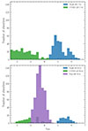 |
Fig. 1. Redshift distribution of absorption features across the three absorber catalogues used in this work. The datasets are indicated in the legend. Note that there are distinctly more C IV absorbers than Si IV absorbers in each dataset. |
3. Analysis
The key quantity used to investigate the clustering of these metal absorbers is the 2PCF (ξ). To calculate this, we first computed the separation between all possible pairs of absorption features of a given species and ionisation state along a certain sightline. We then compared this to the separations that would be expected given a random distribution of absorbers. For each quasar, it is typical to calculate this in a sequence of velocity separation bins. Formally,
 (1)
(1)
where vk = v, v + Δv. n(vk) is the number of absorber pairs in the k-th bin of velocity separation. Subscript R indicates the number of absorber pairs in the same velocity bin based on the random distribution of absorbers. Once summed over all quasars, this is
 (2)
(2)
Here Nqso denotes number of individual sightlines. When looking at C IV from E-XQR-30, Nqso = 42. Note that we calculated the expected number of pairs in each separation bin for each quasar independently. First, we calculated the observed number density of lines across the quasar sample given the total redshift interval of the sample. For each quasar, we then calculated the expected number of lines given the redshift interval spanned by that sightline. The resulting separations were calculated after randomly populating the redshift interval with lines. We ‘threw’ these lines sequentially following a uniform distribution in redshift space. If a line was positioned within 50 km s−1 of a line that had already been generated, it was disregarded and thrown again. This was to ensure we created a random distribution in line with what is observable based on the real X-Shooter data. To understand the uncertainty associated with these calculations, we generated 1000 random realisations of the fake absorption lines. Note that the numerator in Eq. (2) does not change during this process. For each realisation, we calculated the resulting correlation function. This built a distribution of the correlation at each velocity separation that we considered. We then took the median value of this distribution to be representative of the correlation function, and the errors were provided by the interquartile range of the distribution. We did not exclude potential broad absorption line regions in the generated distributions of absorption lines.
We also tested a second approach for computing the distribution of feasible 2PCFs. We adopted a jackknife resampling technique to calculate the range of the 2PCFs given this sample of absorbers. The resulting distributions are indistinguishable from the nominal approach. This indicates that our analysis is not biased by an individual sightline in the sample.
4. Results
Figure 2 shows the resulting 2PCF based on the E-XQR-30 data and the data taken at lower redshift with UVES. In the top panel we show the 2PCF of C IV and Si IV for the lower redshift data before merging the lines to mimic E-XQR-30. This is to highlight the small scales that can be probed with the nominal UVES resolution. The bottom panel shows the clustering of C IV and Si IV based on the E-XQR-30 data.
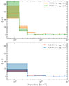 |
Fig. 2. Top: 2PCF of C IV and Si IV based on the UVES LP data analysed in D’Odorico et al. (2010, 2022). In this calculation we have imposed the same column density cuts as applied to the E-XQR-30 data. Compared to E-XQR-30, the resulting distributions are sampled more frequently, with an additional evaluation point at Δv = 150 km s−1. The subsequent bins are consistent with those used for XQR-30. Bottom: 2PCF of C IV and Si IV shown on the smallest scale accessible based on the limited statistics of the Si IV data. The first five bins span Δv = [50 − 300, 300 − 600, 600 − 1200, 1200 − 1500, 1500 − 3000] km s−1. Note that distributions of ξ values are formed via many realisations of the randomly distributed lines. For each sample, the solid line represents the median value and the shaded region encompasses the interquartile range. |
The 2PCFs of C IV and Si IV across both epochs indicate that these metal absorption features are more strongly correlated on small scales compared to a random distribution. This has consistently been found in previous works (Kim et al. 2002; Boksenberg et al. 2003; Boksenberg & Sargent 2015; Scannapieco et al. 2006; D’Odorico et al. 2010). Notably, the clustering falls to zero once the separation reaches scales of 300 − 600 km s−1. At larger velocity separations, the clustering of both the C IV and Si IV absorbers is consistent with what one would expect given a random distribution of metal absorption features.
As the bottom panel of Fig. 2 indicates, the correlation of C IV and Si IV seem to trace one another well on these scales. This has been found at cosmic noon as indicated by the top panel of Fig. 2 (Boksenberg et al. 2003; Scannapieco et al. 2006). For the first time, we highlight that this relationship holds when approaching the end of the epoch of reionization.
4.1. Evolution with redshift
A key motivation to study the clustering of C IV and Si IV using the E-XQR-30 data is to assess whether there is an appreciable redshift evolution in the 2PCF of these metal ionisation states. This has been tentatively seen when analysing data in the redshift interval 2 < z < 4. This has yet to be extended to z > 5. Thus, we now directly compare the results from E-XQR-30 to those at different epochs. This comparison is made after, when necessary, recalibrating the data from other epochs – unlike the data shown in the top panel of Fig. 2.
We initially attempted to assess the potential redshift evolution within the E-XQR-30 survey data. This was approached both by: (1) splitting the sample into two subsamples based on the median absorption redshift, and (2) splitting the sample into two subsamples based on the emission redshift of the quasar. In both cases, we found that they were limited by statistics. There were too few pairs in the subsamples with separations < 1000 km s−1 to make meaningful comparisons across the redshift intervals.
Figure 3 shows the 2PCF of the C IV and Si IV absorbers from the E-XQR-30 survey alongside that computed for the other datasets (described in Sect. 2). In this case, the top panel shows the 2PCF of the C IV data and the bottom panel shows the 2PCF of the Si IV data. Recall that the merged UVES data are denoted as ‘UVES LR’. When considering Si IV, the probed separations of the first five bins are Δv = [50 − 300, 300 − 600, 600 − 1200, 1200 − 1500, 1500 − 3000] km s−1. When considering C IV, we included an additional bin between 50 and 200 km s−1 to probe the smaller separations more effectively (this adjustment means the second bin spans 200 − 300 km s−1).
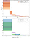 |
Fig. 3. 2PCF of C IV (top) and Si IV (bottom) based on the absorbers in the E-XQR-30 survey now combined with that of the lower redshift ‘UVES LR’ data. The UVES LR data are taken with higher resolution and therefore we have merged the features that would not be resolved with X-Shooter. We additionally include the 2PCF of Si IV from a third dataset, the XQ-100 survey. The shaded region encompasses the interquartile range of the respective distributions. The Si IV absorbers in XQ-100 are found at an intermediate epoch between the XQR-30 and UVES LR data. Note that we can probe down to smaller separations (within 200 km s−1) with C IV due to the increased statistics. |
Overall, this figure highlights that there is no significant difference between the 2PCF of either C IV or Si IV across the epochs traced by the E-XQR-30 ( ) and the UVES LR data (
 ). The median values and associated errors are remarkably consistent. Recall that the shaded region indicates the interquartile range of the distribution. We have additionally confirmed that these distributions are consistent with one another given the 1σ confidence intervals. This is true even on the smallest investigated separations: for C IV this is within 200 km s−1 while for Si IV this is within 300 km s−1. This is perhaps surprising given the tentative redshift evolution that has been found in other works. Though, we note that the errors associated with the bins probing the smallest scales are also relatively large. Another possibility to explain the lack of significant evolution is that differences would become increasingly apparent on even smaller scales than those considered in this figure.
There is a tentative increase in the amplitude of the correlation of the UVES LR data on the scales between 300 and 600 km s−1 compared to that of the E-XQR-30 data that is seen across both C IV and Si IV. This may suggest that the C IV and Si IV systems investigated at z ∼ 2 are tracing more massive structures than their counterparts at higher redshift. Note that, at present, the distributions are consistent with one another within the 2σ confidence intervals. Perhaps with a larger sample of data, this could be determined more precisely for the smallest scales. Indeed, an increase in the completeness of the sample for lower column density absorbers would be an ideal way to build a larger data sample for this analysis. Given the column density distribution of C IV of the E-XQR-30 data (see Fig. 6 of Davies et al. 2023a), reaching a 50 per cent completeness at  would increase the sample size by over one third. Interestingly, the amplitude of the Si IV clustering is also distinctly higher in the XQ-100 sample compared to the E-XQR-30 sample when the separation is between 300 and 600 km s−1. One may have expected the amplitude of this bin to fall between that of E-XQR-30 and the UVES LR sample. It does not and it is consistent with the UVES LR data at the 1σ confidence level.
4.2. Alternative scales
With these data, we were able to construct a robust estimate of the 2PCF of C IV and Si IV towards the end of the epoch of reionization. This is thanks to the extent and quality of the E-XQR-30 data. However, it also poses an interesting question when it comes to comparing these results to those from other redshift intervals. Traditionally, the 2PCF of absorbers is computed as a function of the separation in velocity space (i.e. km s−1). However, the equivalent separation in velocity space will correspond to different physical scales when these epochs are separated by a sufficiently long period in the cosmic history of the Universe. To explore the impact of this, we assumed that the separation between two absorbers in km s−1 is being entirely driven by the motion of the galaxies moving with the Hubble flow. We could then assess what physical scales are being probed by the same velocity separation across different epochs. The minimum resolvable separation in the E-XQR-30 data is Δv = 50 km s−1. Given an average redshift of zabs = 5.1, this corresponds to physical separation of 90 physical kpc. Conversely, this same separation at the average redshift of the UVES LR data (zabs = 2.4) is 200 physical kpc. This may explain the lack of evolution when computing the 2PCF in velocity space.
We next recomputed the 2PCF of these metal absorbers in the reference frame of physical distances. Recall that we assumed a Planck cosmology with H0 = 67.4 ± 0.5 km s−1 Mpc−1, Ωm = 0.315 ± 0.007, and h = 0.677 (Planck Collaboration VI 2020). Similar to what was found in velocity space, we could investigate down to smaller scales when considering C IV alone. However, when considering the behaviour of Si IV, we had to sample the separations more coarsely.
Figure 4 shows the redshift evolution of the 2PCF between  and
and  . This is formatted in the same way as in Fig. 3. Again, the distributions of plausible ξ values for each sample are formed by generating 1000 realisations of the ‘fake’ absorption lines. The resulting distributions are represented by the median value and the interquartile range. For C IV, we investigated to within 800 kpc in the first bin and 800–1500 kpc in the second bin. For Si IV, the first few bins encompass 50 − 1100, 1100 − 2000, and 2000 − 3000 kpc. In the left-hand panel, we compare the 2PCF of C IV from the E-XQR-30 survey to that of the lower redshift UVES LR data. In this reference frame, there is a tentative difference in the clustering of C IV on the smallest scales between these epochs. The amplitude of the UVES LR correlation function is higher than that of the E-XQR-30 data when the separation is within 1500 kpc. For separations < 800 kpc, the significance of the difference is < 1σ. However, there is a ∼2σ difference between the amplitude of the clustering across these epochs for separations between 800 and 1500 kpc. Most notable, the clustering of the lower redshift absorbers seems to extend to larger separations than that of the E-XQR-30 data. On these scales, the relative impact of the peculiar velocities of the absorbers should not have a substantial impact. Indeed, it has been found (albeit at z ∼ 2) that beyond 300 kpc the line-of-sight kinematics of H I are dominated by Hubble expansion (Chen et al. 2020). Within the scale of the first bin, there is likely to be a contribution from galaxies within a single halo as will be discussed in Sect. 5.2.
 |
Fig. 4. Left: 2PCF of C IV as a function of the separation between pairs in physical kpc space. The legend indicates the different data samples. Right: Same as the left panel but now showing Si IV. For C IV the first bin encompasses everything within 800 kpc. For Si IV, the first bin encompasses everything within 1100 kpc. In both panels, the shaded region encompasses the interquartile range of the distributions. |
The right-hand panel of Fig. 4 shows the 2PCF of Si IV based on three data samples that span three redshift intervals. These data show a similar trend to that found for C IV; however, the errors associated with UVES LR data make it challenging to draw firm conclusions on the smallest separations at the lowest redshifts. The E-XQR-30 and XQ-100 data show a significant difference in the amplitude at the smallest separations (< 1100 kpc). This follows the trend seen in C IV, highlighting two key results: (1) The C IV and Si IV trace one another closely when considering separations the reference frame of physical kpc, (2) The amplitude of the clustering of the C IV and Si IV absorbers increases on the smallest scales as we investigate closer to the present day. This may suggest that the metal absorption line systems are found in denser environments at lower redshifts compared to higher redshifts. Though, we note that his evolution might also be influenced by the evolution of the ionising UV background (UVB). During the epoch of reionization, the UVB is patchy and dominated by local sources like young galaxies and early quasars. This confines ionised metals to small and localised regions. At cosmic noon, however, the UVB becomes stronger and more uniform, allowing metals to be ionised over larger physical scales, including diffuse regions of the IGM (Khaire & Srianand 2019). This leads to the enhanced spatial clustering of C IV and Si IV absorbers as they begin to trace the large-scale structure of the cosmic web. It is important to recognise that the observed evolution reflects the combined impacts of the UVB evolution, large-scale structure growth, and the increasing dispersal of metals into the IGM and CGM over cosmic time.
5. Discussion
Fundamentally, one would like to understand where the gas being analysed arises with respect to the galaxy populations at these different epochs. In principle, the observed evolution in the 2PCF should be reproducible in cosmological hydrodynamical simulations. This would provide an indirect means to associate these metal absorbers with their place within the cosmic web of structure formation. This will be discussed further in Sect. 5.2. First we discuss how these results compare to other observations.
It has been appreciated for multiple decades that the 2PCF of Lyα absorbers shows a significant signal on small velocity scales (i.e. Δv ∼ 300 km s−1) with both the amplitude and significance increasing with increasing column density (e.g. Cristiani et al. 1997). At this time, the correlation scale at z ∼ 3 was found to be 150 − 220 h−1 comoving kpc with an apparent trend of increasing correlation with decreasing redshift. This was reaffirmed with a larger sample of data covering 1.5 < z < 4 (Kim et al. 2001). Wolfson et al. (2023) have recently extended this investigation to earlier epochs. They utilise the E-XQR-30 sample to forecast the mean free path of ionising photons at z > 5.7 based on the Lyα forest flux autocorrelation function. In Wolfson et al. (2024), they further compute the autocorrelation function of the Lyα transmission normalised and shifted by the mean transmission in ten redshift bins and find a significant signal for most redshift bins on small scales (Δv ∼ 200 km s−1). We find a significant signal on similar scales when investigating the E-XQR-30 C IV absorbers. Thus, these works provide independent yet complementary approaches to studying the clustering of structure using these quasar absorption line data. It is interesting to note that the trend of increasing correlation with decreasing redshift is consistent with our analysis using metal absorbers in place of Lyα absorption.
In addition to Lyα absorption, one can compare how the 2PCF of C IV and Si IV behaves relative to that of different galaxy types at these epochs. Observationally, the correlation of galaxy types at high redshift has become more accessible thanks to the James Webb Space Telescope (JWST). At more recent epochs, there have been many pioneering studies of galaxy correlations (e.g. Adelberger et al. 2005), some of which even compare the galaxy–galaxy and galaxy–absorber correlations (see Sect. 5.1).
In particular, JWST-NIRCam has facilitated the photometric selection of Lyman-break galaxies out to unparalleled epochs. Dalmasso et al. (2024) uses the JWST Advanced Deep Extragalactic Survey (JADES) to characterise the galaxy–galaxy correlation function out to z ∼ 11. This work utilises the angular correlation function and the galaxy bias as a measure of the clustering. Once complete, the JADES survey will be optimal for identifying robust z > 15 galaxy candidates (Eisenstein et al. 2023). At redshifts similar to that of the E-XQR-30 data, the clustering of [O III] and H β emitting galaxies has been characterised by the Emission-line galaxies and Intergalactic Gas in the Epoch of reionization (EIGER) survey (Matthee et al. 2023). Using the angular correlation of the observed galaxies, they find an excess of small-scale clustering when the separation is < 2 arcseconds. These galaxies are found to have stellar masses in the range M⋆ = 106.8 − 10.1 M⊙. While this separation is smaller (∼10 kpc) than the scales considered in this work, the results are consistent with the trend of increased clustering at smaller separations.
A complementary statistic is the transverse autocorrelation function of absorption features. This provides information beyond the dimensions of an individual line of sight. At cosmic noon this has been investigated using C IV and Lyα features. For example, at 2 < z < 3, the transverse autocorrelation of C IV absorbers has been calculated using close quasar pairs (Mintz et al. 2022). This work finds that the transverse autocorrelation function appears to level off at ∼200 h−1 comoving kpc (see their Fig. 8). Assuming that the C IV absorbers identified in the spectra of both members of the quasar pairs arise from the same structure, this indicates that the structures being traced by C IV are at least ∼200 h−1 comoving kpc in size. A similar study has been conducted using Lyα absorbers detected in the spectra of quasar pairs at z ∼ 2 (D’Odorico et al. 2006). This indicates that the clustering of H I bearing gas is significant up to ∼3 h−1 comoving Mpc. This work also finds good agreement between the line of sight and transverse autocorrelation, suggesting that the potential impact of galaxy motions along the line of sight are minimal. This type of analysis has yet to be extended to the epochs covered by the E-XQR-30 data.
5.1. Galaxy–absorber associations
To unravel the potential similarities between galaxy–galaxy correlations and absorber–absorber correlations, the detection of gas around galaxies can provide a bridge between these statistics. As with the transverse correlation function, they can also provide a direct determination of the physical extent of gas surrounding galaxies. Above z > 4, MUSE has been utilised to search for galaxies associated with C IV absorbers (Díaz et al. 2021). At these redshifts, stronger C IV systems are more likely to have Lyα-emitting galaxies within 200 proper kpc. This association of galaxies and strong C IV systems is also seen in the EIGER survey (Kashino et al. 2023). This is again similar to the clustering scales observed through the 2PCF of C IV absorbers in the E-XQR-30 sample.
Using JWST, A SPectroscopic survey of biased halos In the reionization Era (ASPIRE) has found a high incidence rate of galaxies detected within 1000 km s−1 and 350 kpc of known absorbers in the redshift interval 6.0 < zabs < 6.5. These absorbers are typically detected in both C II and C IV while the galaxies are detected through [O III] and H β (Zou et al. 2024). Comparing this to the clustering of C IV absorbers in the E-XQR-30 survey, we see an increase in the correlations of absorbers on similar physical kpc scales. There is no evidence to indicate that there is an intrinsic difference between the structures traced by the strong C IV systems in the E-XQR-30 data and the galaxy-absorber pairs from ASPIRE. An independent study of galaxies associated with Mg II absorbers at this epoch would suggest a highly efficient enrichment of the IGM at the end of reionization (Bordoloi et al. 2024); this has been found through analysing the same field that has been used in Kashino et al. (2023) while the results presented in Zou et al. (2024) are based on the analysis of four independent fields.
5.2. Perspective from galaxy simulations
Simulations of the formation and evolution of galaxies are an ideal benchmark of comparison for these observational data and the resulting clustering analysis. These comparisons are particularly useful to understand the possible structures giving rise to the observed clustering between absorbers. It is also uniquely suited to disentangling the contribution of different sources to the evolution in the clustering; in simulations, the systematics are well understood and the contribution of different physical processes (e.g. the evolution of the mean density, the metallicity, and the size of galaxy halos) can be directly determined.
With the latest generation of spectroscopic surveys (e.g. DESI, WEAVE, and 4MOST; Dalton et al. 2012; de Jong et al. 2012; DESI Collaboration 2024; Jin et al. 2024), combined with the launch of Euclid and JWST, there has been an increase in the endeavour to map the correlation function of galaxies at increasingly high redshift through simulations (e.g. Euclid Collaboration: Böhringer et al. 2025; Euclid Collaboration: Castander et al. 2025; Pizzati et al. 2024). For the purpose of this work, we looked to the galaxy clustering as produced through the GAEA semi-analytical galaxy formation model (De Lucia et al. 2024). This model utilises merger trees extracted from the P-Millennium Simulation (Baugh et al. 2019) and has recently been used to explore the clustering of galaxies at 0 < z < 5 (Fontanot et al. 2025). The model also covers the epochs considered in our analysis, in particular, z = 2.46 and z = 5.20. These roughly correspond to the epochs traced by the low-redshift UVES LR data and the E-XQR-30 data. We note that the simulations adopt the same cosmology as used in this work.
The CORRFUNC python package can be used to estimate the projected correlation of simulated galaxies based on their position and redshift (Sinha & Garrison 2020). We considered the correlation of all galaxies in the snapshot as well as the correlation of only the central galaxies. When including satellites, we made no distinction between type-1 and orphan satellites (those whose substructure is stripped below the resolution limit of the simulation; De Lucia et al. 2019). While our analysis relies on the correlation along the line of sight, this can still be used to draw parallels between what we observe and simulations. In this scenario, we are comparing the galaxy–galaxy clustering from simulation snapshots to the absorber–absorber clustering from quasar sightlines.
Using CORRFUNC, we computed the 3D real space correlation as a function of the radial position in comoving Mpc. We find that the amplitude of the clustering at a given epoch increases when tracing galaxies with increasing stellar mass. This behaviour is also seen when tracing galaxies embedded in increasingly massive halos as traced by the virial parent halo mass. This can be seen in Fig. 5. In this figure, we show the correlation of all galaxies associated with a given virial mass (solid line) as well as the correlation of only the central galaxies associated with a given halo (dotted line). As expected, the correlation of the central galaxies drops off at the smallest separations while the correlation between all the detected galaxies does not. This is well documented in the literature. It can be understood in terms of the halo model – namely, at small scales the main contribution to the clustering signal is coming from the ‘one-halo’ term, i.e. from galaxies that are sitting within the same halo, while at larger scales what dominates is the ‘two-halo’ term, i.e. the signal is driven by (central) galaxies that are sitting in different halos. The increase in the amplitude of the correlation is also understood to increase with luminosity (which, for central galaxies, can be a proxy of halo mass). For a given virial mass, the amplitude of the correlation is stronger for galaxies at high redshift compared to their lower redshift counterparts. This is true at separation scales larger than r = 0.3 h−1 Mpc. We highlight a comparison of each mass bin across the different epochs in Appendix A.
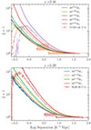 |
Fig. 5. 3D real space correlation calculated at different epochs using the GAEA simulation suite snapshots. The correlation is calculated using the CORRFUNC package. The different colours correspond to galaxies with different virial parent halo masses. The top and bottom panels correspond to different epochs, as indicated by the titles. The solid curves represent the clustering of all galaxies in the snapshot. The dotted lines represent that of only the central galaxies associated with halos. The observed 2PCFs of C IV and Si IV have been overplotted on these simulation data across different epochs. In this case, we calculated the 2PCF of C IV systems (i.e. all the absorption within 200 km s−1 is considered one feature). Again, the shaded regions correspond to the interquartile range of the observed distributions. |
Since the separation between these simulated galaxies is calculated in the reference frame of comoving Mpc, we recomputed the 2PCF of C IV in this reference frame. The results of this are overplotted on the simulation data in Fig. 5. In this coordinate system, the E-XQR-30 data can probe scales as small as ∼0.36 h−1 Mpc assuming a median redshift of z = 5.1. The merged UVES data can probe scales of ∼0.47 h−1 Mpc. Notably, in this case we also did not consider the individual absorbers. Instead, we considered the 2PCF of absorption line ‘systems’ as defined in Davies et al. (2023a). These systems are defined as all of the absorption within 200 km s−1. We emulated this in the UVES data by merging all of the absorption line features of C IV that fall within 200 km s−1 of one another. Following the process described in Sect. 2, these systems are merged into one absorber with a column density equivalent to the sum of the original lines and a redshift that is the column-density-weighted average of the lines. This choice ensures that the signal we are comparing to the simulations is not dominated by the contribution from absorbers within the same halo.
The comparison of the observational data and the simulated galaxy correlation in Fig. 5 showcases that the intensity of the correlation as traced by the 3D simulation information of central galaxies is comparable to that traced by C IV absorption line systems at z ∼ 5.1 and at z ∼ 2.4; this is true on all the scales probed. The smallest separations that we tested at each epoch suggest that we are not reaching the scales necessary to probe the correlation of substructures within a given halo. This, in part, motivates our choice to consider absorption line ‘systems’. The amplitude of the correlation at both z = 2.46 and z = 5.20 for the simulated halos with virial masses M ∼ 1010.5 M⊙ are the most similar to the trends seen in the real data at these epochs. Overall, we find a consistency between the galaxy–galaxy clustering seen in these simulations and the absorber–absorber clustering seen in the E-XQR-30 data.
In Fig. 6 we show the halo mass function of galaxies at the two epochs spanned by the E-XQR-30 and UVES LR data. Given the density of structures in these simulations, this function is sensitive to halo masses up to  ; this corresponds to a number density per unit mass of dN/dM ∼ 10−20. As expected, this figure highlights that there are fewer halos with high masses at high redshift compared to lower redshift. It is important to consider how this sensitivity may change across epochs since the structures we are tracing with the C IV and Si IV absorbers may be associated with the least massive halos.
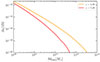 |
Fig. 6. Halo mass function of galaxies from GAEA at the two epochs spanned by the XQR-30 and UVES LR data. This highlights that there are relatively more galaxies of a given halo mass at the epoch explored by the UVES LR data than the epoch explored for the XQR-30 data. This difference becomes more apparent for the highest-mass halos. |
These qualitative comparisons can provide insight into the nature of the sources that produce the C IV systems observed through E-XQR-30. In the future, the use of synthetic sightlines will allow for a direct comparison with simulations that contain radiative transfer and hydrodynamics (Springel et al. 2018; Garaldi et al. 2022). Following the evolution of the 2PCF of C IV for different halos in these simulations and comparing that to the real data will allow us to determine the properties of the halos that best reproduce these data. Of particular interest is the typical size of the enriched region around a typical z = 5.1 galaxy compared to that at lower redshifts. This may provide insight into the size of the CGM across cosmic time. Further, comparisons with the predicted size of pristine and/or Population III enriched bubbles (e.g. Hartwig et al. 2024) could highlight the diversity in the scale of enriched gas at this epoch. This is motivated by the likelihood that the Pop. III enriched regions are likely some of the smaller structures at this epoch compared to those traced by strong C IV or Si IV absorption.
6. Conclusions
We used the E-XQR-30 dataset to investigate the clustering of C IV and Si IV close to the epoch of reionization using the 2PCF. We compared these results to those found at later epochs to assess the potential redshift evolution of this clustering. We then drew comparisons with the galaxy clustering properties from the GAEA semi-analytical galaxy formation model. Our main conclusions are as follows:
-
We find that the clustering as described by the 2PCF of C IV absorbers is indistinguishable between the epoch explored by the E-XQR-30 survey (
 ) and a compilation of quasars observed with UVES at cosmic noon (
 ) when evaluating the separation of absorbers in velocity space.
 -
This is also true when considering the 2PCF of Si IV absorbers. For Si IV, we additionally considered a catalogue of absorbers from the XQ-100 survey (
 ).
). -
The difference in the 2PCF becomes significant when tracing absorbers on physical kiloparsec scales rather than velocity separation. We find an indication that the amplitude of the correlation increases at lower redshift when considering scales < 1500 physical kpc. This is consistent with previous works.
-
We compared these results to the GAEA semi-analytic galaxy formation model. We compared the evolution of the correlation function from z = 5.20 to z = 2.46 as a function of the virial mass of halos. We find that the correlation signal of the galaxies is broadly consistent with the observed data. This is after accounting for the possibility that the dominant source of the observed clustering between absorbers is due to the contribution of gas within the same halo.
-
We propose that a semi-analytic model of galaxy formation tailored towards understanding the 2PCF of absorbers may provide insight into the size of the CGM and the level of metal enrichment at epochs close to the end of reionization.
The metal absorbers detected towards the end of the reionization epoch are invaluable tracers of cosmic structure. With the next generation of ground-based facilities, for example the Extremely Large Telescope (ELT), we will reach an unprecedented sensitivity when observing high redshift quasars. In particular, the ELT-ANDES high-resolution spectrograph will be critical to detecting the low column density absorbers with a confidence that is inaccessible with current instruments (D’Odorico et al. 2024).
Acknowledgments
We thank the anonymous referee for their thoughtful feedback and suggestions that improved the quality of this manuscript. We thank the organisers and participants of the Baryons Beyond Galactic Boundaries 2024 conference for helpful discussions and feedback. LW and VD acknowledges financial support from the Bando Ricerca Fondamentale INAF 2022 Large Grant “XQR-30”. SEIB is supported by the Deutsche Forschungsgemeinschaft (DFG) under Emmy Noether grant number BO 5771/1-1. RLD is supported by the Australian Research Council through the Discovery Early Career Researcher Award (DECRA) Fellowship DE240100136 funded by the Australian Government. This research was supported in part by the Australian Research Council Centre of Excellence for All Sky Astrophysics in 3 Dimensions (ASTRO 3D), through project number CE170100013. This paper is based on observations collected at the European Organisation for Astronomical Research in the Southern Hemisphere, Chile. We are grateful to the staff astronomers at the VLT for their assistance with the observations. This research has made use of NASA’s Astrophysics Data System.
References
- Adelberger, K. L., Shapley, A. E., Steidel, C. C., et al. 2005, ApJ, 629, 636 [NASA ADS] [CrossRef] [Google Scholar]
- Bañados, E., Venemans, B. P., Decarli, R., et al. 2016, ApJS, 227, 11 [Google Scholar]
- Baugh, C. M., Gonzalez-Perez, V., Lagos, C. D. P., et al. 2019, MNRAS, 483, 4922 [NASA ADS] [CrossRef] [Google Scholar]
- Becker, G. D., Rauch, M., & Sargent, W. L. W. 2009, ApJ, 698, 1010 [CrossRef] [Google Scholar]
- Becker, G. D., Pettini, M., Rafelski, M., et al. 2019, ApJ, 883, 163 [NASA ADS] [CrossRef] [Google Scholar]
- Bird, S., Rubin, K. H. R., Suresh, J., & Hernquist, L. 2016, MNRAS, 462, 307 [NASA ADS] [CrossRef] [Google Scholar]
- Bischetti, M., Feruglio, C., D’Odorico, V., et al. 2022, Nature, 605, 244 [NASA ADS] [CrossRef] [Google Scholar]
- Boksenberg, A., & Sargent, W. L. W. 2015, ApJS, 218, 7 [NASA ADS] [CrossRef] [Google Scholar]
- Boksenberg, A., Sargent, W. L. W., & Rauch, M. 2003, ApJS, submitted [arXiv:astro-ph/0307557] [Google Scholar]
- Bordoloi, R., Simcoe, R. A., Matthee, J., et al. 2024, ApJ, 963, 28 [NASA ADS] [CrossRef] [Google Scholar]
- Bosman, S. E. I., Becker, G. D., Haehnelt, M. G., et al. 2017, MNRAS, 470, 1919 [NASA ADS] [CrossRef] [Google Scholar]
- Chen, Y., Steidel, C. C., Hummels, C. B., et al. 2020, MNRAS, 499, 1721 [NASA ADS] [CrossRef] [Google Scholar]
- Christensen, L., Jakobsen, P., Willott, C., et al. 2023, A&A, 680, A82 [NASA ADS] [CrossRef] [EDP Sciences] [Google Scholar]
- Cowie, L. L., Songaila, A., Kim, T.-S., & Hu, E. M. 1995, AJ, 109, 1522 [NASA ADS] [CrossRef] [Google Scholar]
- Cristiani, S., D’Odorico, S., D’Odorico, V., et al. 1997, MNRAS, 285, 209 [Google Scholar]
- Dalmasso, N., Leethochawalit, N., Trenti, M., & Boyett, K. 2024, MNRAS, 533, 2391 [Google Scholar]
- Dalton, G., Trager, S. C., & Abrams, D. C. 2012, in Ground-based and Airborne Instrumentation for Astronomy IV, eds. I. S. McLean, S. K. Ramsay, & H. Takami, SPIE Conf. Ser., 8446, 84460P [NASA ADS] [Google Scholar]
- Davies, R. L., Ryan-Weber, E., D’Odorico, V., et al. 2023a, MNRAS, 521, 289 [NASA ADS] [CrossRef] [Google Scholar]
- Davies, R. L., Ryan-Weber, E., D’Odorico, V., et al. 2023b, MNRAS, 521, 314 [NASA ADS] [CrossRef] [Google Scholar]
- de Jong, R. S., Bellido-Tirado, O., Chiappini, C., et al. 2012, in Ground-based and Airborne Instrumentation for Astronomy IV, eds. I. S. McLean, S. K. Ramsay, & H. Takami, SPIE Conf. Ser., 8446, 84460T [NASA ADS] [Google Scholar]
- De Lucia, G., Hirschmann, M., & Fontanot, F. 2019, MNRAS, 482, 5041 [Google Scholar]
- De Lucia, G., Fontanot, F., Xie, L., & Hirschmann, M. 2024, A&A, 687, A68 [NASA ADS] [CrossRef] [EDP Sciences] [Google Scholar]
- Dekker, H., D’Odorico, S., Kaufer, A., Delabre, B., & Kotzlowski, H. 2000, in Optical and IR Telescope Instrumentation and Detectors, eds. M. Iye, & A. F. Moorwood, Proc. SPIE, 4008, 534 [Google Scholar]
- DESI Collaboration (Adame, A. G., et al.) 2024, AJ, 168, 58 [NASA ADS] [CrossRef] [Google Scholar]
- Díaz, C. G., Ryan-Weber, E. V., Cooke, J., Pettini, M., & Madau, P. 2011, MNRAS, 418, 820 [Google Scholar]
- Díaz, C. G., Ryan-Weber, E. V., Karman, W., et al. 2021, MNRAS, 502, 2645 [CrossRef] [Google Scholar]
- D’Odorico, V., Viel, M., Saitta, F., et al. 2006, MNRAS, 372, 1333 [Google Scholar]
- D’Odorico, V., Calura, F., Cristiani, S., & Viel, M. 2010, MNRAS, 401, 2715 [Google Scholar]
- D’Odorico, V., Cupani, G., Cristiani, S., et al. 2013, MNRAS, 435, 1198 [CrossRef] [Google Scholar]
- D’Odorico, V., Finlator, K., Cristiani, S., et al. 2022, MNRAS, 512, 2389 [CrossRef] [Google Scholar]
- D’Odorico, V., Bañados, E., Becker, G. D., et al. 2023, MNRAS, 523, 1399 [CrossRef] [Google Scholar]
- D’Odorico, V., Bolton, J. S., Christensen, L., et al. 2024, Exp. Astron., 58, 21 [Google Scholar]
- Doughty, C. C., & Finlator, K. M. 2023, MNRAS, 518, 4159 [Google Scholar]
- Eisenstein, D. J., Johnson, B. D., Robertson, B., et al. 2023, ArXiv e-prints [arXiv:2310.12340] [Google Scholar]
- Euclid Collaboration (Böhringer, H., et al.) 2025, A&A, 693, A59 [Google Scholar]
- Euclid Collaboration (Castander, F. J., et al.) 2025, A&A, 697, A5 [Google Scholar]
- Finlator, K., Doughty, C., Cai, Z., & Díaz, G. 2020, MNRAS, 493, 3223 [NASA ADS] [CrossRef] [Google Scholar]
- Fiore, F., Ferrara, A., Bischetti, M., Feruglio, C., & Travascio, A. 2023, ApJ, 943, L27 [NASA ADS] [CrossRef] [Google Scholar]
- Fontanot, F., De Lucia, G., Xie, L., et al. 2025, A&A, 699, A108 [NASA ADS] [CrossRef] [EDP Sciences] [Google Scholar]
- Garaldi, E., Kannan, R., Smith, A., et al. 2022, MNRAS, 512, 4909 [NASA ADS] [CrossRef] [Google Scholar]
- Hartwig, T., Lipatova, V., Glover, S. C. O., & Klessen, R. S. 2024, MNRAS, 535, 516 [Google Scholar]
- Jin, S., Trager, S. C., Dalton, G. B., et al. 2024, MNRAS, 530, 2688 [NASA ADS] [CrossRef] [Google Scholar]
- Kashino, D., Lilly, S. J., Matthee, J., et al. 2023, ApJ, 950, 66 [CrossRef] [Google Scholar]
- Khaire, V., & Srianand, R. 2019, MNRAS, 484, 4174 [NASA ADS] [CrossRef] [Google Scholar]
- Kim, T. S., Cristiani, S., & D’Odorico, S. 2001, A&A, 373, 757 [NASA ADS] [CrossRef] [EDP Sciences] [Google Scholar]
- Kim, T. S., Cristiani, S., & D’Odorico, S. 2002, A&A, 383, 747 [NASA ADS] [CrossRef] [EDP Sciences] [Google Scholar]
- Lopez, S., Afruni, A., Zamora, D., et al. 2024, A&A, 691, A356 [NASA ADS] [CrossRef] [EDP Sciences] [Google Scholar]
- López, S., D’Odorico, V., Ellison, S. L., et al. 2016, A&A, 594, A91 [NASA ADS] [CrossRef] [EDP Sciences] [Google Scholar]
- Lu, L. 1991, ApJ, 379, 99 [Google Scholar]
- Matthee, J., Mackenzie, R., Simcoe, R. A., et al. 2023, ApJ, 950, 67 [NASA ADS] [CrossRef] [Google Scholar]
- Mintz, A., Rafelski, M., Jorgenson, R. A., et al. 2022, AJ, 164, 51 [NASA ADS] [CrossRef] [Google Scholar]
- Péroux, C., & Howk, J. C. 2020, ARA&A, 58, 363 [CrossRef] [Google Scholar]
- Pettini, M., Madau, P., Bolte, M., et al. 2003, ApJ, 594, 695 [NASA ADS] [CrossRef] [Google Scholar]
- Pizzati, E., Hennawi, J. F., Schaye, J., et al. 2024, MNRAS, 534, 3155 [Google Scholar]
- Planck Collaboration VI. 2020, A&A, 641, A6 [NASA ADS] [CrossRef] [EDP Sciences] [Google Scholar]
- Ryan-Weber, E. V., Pettini, M., & Madau, P. 2006, MNRAS, 371, L78 [NASA ADS] [CrossRef] [Google Scholar]
- Ryan-Weber, E. V., Pettini, M., Madau, P., & Zych, B. J. 2009, MNRAS, 395, 1476 [NASA ADS] [CrossRef] [Google Scholar]
- Scannapieco, E., Pichon, C., Aracil, B., et al. 2006, MNRAS, 365, 615 [NASA ADS] [CrossRef] [Google Scholar]
- Sebastian, A. M., Ryan-Weber, E., Davies, R. L., et al. 2024, MNRAS, 530, 1829 [NASA ADS] [CrossRef] [Google Scholar]
- Simcoe, R. A. 2006, ApJ, 653, 977 [CrossRef] [Google Scholar]
- Sinha, M., & Garrison, L. H. 2020, MNRAS, 491, 3022 [Google Scholar]
- Songaila, A. 2001, ApJ, 561, L153 [NASA ADS] [CrossRef] [Google Scholar]
- Springel, V., Pakmor, R., Pillepich, A., et al. 2018, MNRAS, 475, 676 [Google Scholar]
- Steidel, C. C., Erb, D. K., Shapley, A. E., et al. 2010, ApJ, 717, 289 [Google Scholar]
- Tescari, E., Viel, M., D’Odorico, V., et al. 2011, MNRAS, 411, 826 [NASA ADS] [CrossRef] [Google Scholar]
- Tortosa, A., Zappacosta, L., Piconcelli, E., et al. 2024, A&A, 691, A235 [NASA ADS] [CrossRef] [EDP Sciences] [Google Scholar]
- Tumlinson, J., Peeples, M. S., & Werk, J. K. 2017, ARA&A, 55, 389 [Google Scholar]
- Vernet, J., Dekker, H., D’Odorico, S., et al. 2011, A&A, 536, A105 [NASA ADS] [CrossRef] [EDP Sciences] [Google Scholar]
- Wolfson, M., Hennawi, J. F., Davies, F. B., & Oñorbe, J. 2023, MNRAS, 521, 4056 [Google Scholar]
- Wolfson, M., Hennawi, J. F., Bosman, S. E. I., et al. 2024, MNRAS, 531, 3069 [NASA ADS] [CrossRef] [Google Scholar]
- Yang, J., Fan, X., Gupta, A., et al. 2023, ApJS, 269, 27 [NASA ADS] [CrossRef] [Google Scholar]
- Zou, S., Cai, Z., Wang, F., et al. 2024, ApJ, 963, L28 [Google Scholar]
Appendix A: Clustering over time for a given halo mass
In this appendix we highlight how the clustering of structure evolves from the epoch of reionization to cosmic noon for galaxies of increasing virial parent halo masses. This is highlighted in Fig. A.1. The increasing amplitude of the correlation at higher redshifts is well documented in the literature.
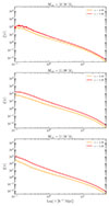 |
Fig. A.1. Clustering of structures across different cosmic epochs. The different rows show this clustering for galaxies within different halo mass bins. |
All Figures
|
Fig. 1. Redshift distribution of absorption features across the three absorber catalogues used in this work. The datasets are indicated in the legend. Note that there are distinctly more C IV absorbers than Si IV absorbers in each dataset. |
| In the text | |
|
Fig. 2. Top: 2PCF of C IV and Si IV based on the UVES LP data analysed in D’Odorico et al. (2010, 2022). In this calculation we have imposed the same column density cuts as applied to the E-XQR-30 data. Compared to E-XQR-30, the resulting distributions are sampled more frequently, with an additional evaluation point at Δv = 150 km s−1. The subsequent bins are consistent with those used for XQR-30. Bottom: 2PCF of C IV and Si IV shown on the smallest scale accessible based on the limited statistics of the Si IV data. The first five bins span Δv = [50 − 300, 300 − 600, 600 − 1200, 1200 − 1500, 1500 − 3000] km s−1. Note that distributions of ξ values are formed via many realisations of the randomly distributed lines. For each sample, the solid line represents the median value and the shaded region encompasses the interquartile range. |
| In the text | |
|
Fig. 3. 2PCF of C IV (top) and Si IV (bottom) based on the absorbers in the E-XQR-30 survey now combined with that of the lower redshift ‘UVES LR’ data. The UVES LR data are taken with higher resolution and therefore we have merged the features that would not be resolved with X-Shooter. We additionally include the 2PCF of Si IV from a third dataset, the XQ-100 survey. The shaded region encompasses the interquartile range of the respective distributions. The Si IV absorbers in XQ-100 are found at an intermediate epoch between the XQR-30 and UVES LR data. Note that we can probe down to smaller separations (within 200 km s−1) with C IV due to the increased statistics. |
| In the text | |
|
Fig. 4. Left: 2PCF of C IV as a function of the separation between pairs in physical kpc space. The legend indicates the different data samples. Right: Same as the left panel but now showing Si IV. For C IV the first bin encompasses everything within 800 kpc. For Si IV, the first bin encompasses everything within 1100 kpc. In both panels, the shaded region encompasses the interquartile range of the distributions. |
| In the text | |
|
Fig. 5. 3D real space correlation calculated at different epochs using the GAEA simulation suite snapshots. The correlation is calculated using the CORRFUNC package. The different colours correspond to galaxies with different virial parent halo masses. The top and bottom panels correspond to different epochs, as indicated by the titles. The solid curves represent the clustering of all galaxies in the snapshot. The dotted lines represent that of only the central galaxies associated with halos. The observed 2PCFs of C IV and Si IV have been overplotted on these simulation data across different epochs. In this case, we calculated the 2PCF of C IV systems (i.e. all the absorption within 200 km s−1 is considered one feature). Again, the shaded regions correspond to the interquartile range of the observed distributions. |
| In the text | |
|
Fig. 6. Halo mass function of galaxies from GAEA at the two epochs spanned by the XQR-30 and UVES LR data. This highlights that there are relatively more galaxies of a given halo mass at the epoch explored by the UVES LR data than the epoch explored for the XQR-30 data. This difference becomes more apparent for the highest-mass halos. |
| In the text | |
|
Fig. A.1. Clustering of structures across different cosmic epochs. The different rows show this clustering for galaxies within different halo mass bins. |
| In the text | |
Current usage metrics show cumulative count of Article Views (full-text article views including HTML views, PDF and ePub downloads, according to the available data) and Abstracts Views on Vision4Press platform.
Data correspond to usage on the plateform after 2015. The current usage metrics is available 48-96 hours after online publication and is updated daily on week days.
Initial download of the metrics may take a while.