| Issue |
A&A
Volume 703, November 2025
|
|
|---|---|---|
| Article Number | A120 | |
| Number of page(s) | 13 | |
| Section | Planets, planetary systems, and small bodies | |
| DOI | https://doi.org/10.1051/0004-6361/202554487 | |
| Published online | 07 November 2025 | |
Volatile distribution inversion and rotation analysis of comet 103P/Hartley 2 using nongravitational effects
1
School of Astronautics, Beihang University,
100191
Beijing,
China
2
Key Laboratory of Spacecraft Design Optimization and Dynamic Simulation Technologies, Ministry of Education,
100191
Beijing,
China
3
Institute of Mechanics, Chinese Academy of Science,
100190
Beijing,
China
★ Corresponding author: This email address is being protected from spambots. You need JavaScript enabled to view it.
Received:
12
March
2025
Accepted:
24
September
2025
Abstract
Aims. The rotational states of comet 103P/Hartley 2 (103P) during its perihelion passage are strongly modulated by nongravitational forces. By fitting its attitude-variation measurements, this study aims to infer the spatial distributions of H2O and CO2 ices on the nucleus and to assess how these inhomogeneities drive the nucleus’s rotational behavior.
Methods. We adopted a dust-mantle thermal model of the nucleus that incorporates H2O and CO2 ices as the principal volatiles. A coupled attitude-thermal simulation framework was developed, in which a neural-network surrogate greatly accelerates the iterative computations. The nucleus was partitioned into three morphological regions – large end, waist, and small end – and a localized activity model described the uneven sublimation across these zones.
Results. Our model successfully reproduces both the observed rotational variations and the measured volatile production rates of 103P during its 2010 encounter. At the observation instant, in addition to the pronounced CO2 sublimation at the sunlit small end, the dust mantle covering the large end insulated the underlying CO2, allowing it to continue sublimating on the shadowed side. We find that the H2O ice-front depth is on the order of millimeters, whereas the CO2 ice front lies between centimeters and decimeters, with the large end exhibiting stronger activity. The fitted CO2 production rate closely matches the observations, while direct H2O sublimation contributes only a minor fraction. The total H2O production rate of 103P may primarily originate from H2O ice ejected by CO2 sublimation at the nucleus’s ends. Moreover, CO2 sublimation at the large end produces the majority of the recoil torque, driving the nucleus’s enhanced long-axis excitation following the encounter.
Key words: solid state: volatile / methods: numerical / comets: general / comets: individual: 103P/Hartley 2
© The Authors 2025
 Open Access article, published by EDP Sciences, under the terms of the Creative Commons Attribution License (https://creativecommons.org/licenses/by/4.0), which permits unrestricted use, distribution, and reproduction in any medium, provided the original work is properly cited.
This article is published in open access under the Subscribe to Open model. This email address is being protected from spambots. You need JavaScript enabled to view it. to support open access publication.
1 Introduction
Comets are typically in a low solar radiation environment, preserving relatively primitive compositions and structures within their interiors (Bockelée-Morvan et al. 2004). Understanding the physical properties of comets helps us to gain deeper insights into the early evolutionary history of the Solar System.
As comets approach the Sun, the solar radiation causes sublimation of volatiles such as H2O ice and CO2 ice on their surfaces, which in turn leads to the escape of refractory particles from the nucleus, forming the coma and the tail. During this process, the comet also exhibits significant nongravitational effects (hereafter NGEs). Serving as the critical interface between the comet’s thermal state and its orbital and rotational dynamics, these NGEs play a crucial role in governing cometary activity and long-term evolution.
On the one hand, the NGEs generated by the recoil from sublimating volatiles influence the comet’s attitude and orbital motion. As volatiles sublimate from the nucleus surface, the out-gassing exerts a recoil force on the nucleus, which alters its orbit and attitude (Marsden 2009). Encke first observed the deviation of the orbit of comet 2P/Encke from the Keplerian orbit (Encke 1821). To more accurately predict the comet’s motion, Marsden added a nongravitational acceleration (hereafter NGA) term to the Kepler model (Marsden 1969) and described the variation of water ice sublimation with the heliocentric distance through an empirical function (Marsden et al. 1973). This model has become the “standard model” for studying cometary orbital motion. Marsden analyzed the orbits of 79 Jupiter-family comets with nongravitational perturbations, and the results indicated that the NGAs acting on comets primarily originate from the sublimation of water ice (Marsden 2009). Due to the asymmetric shape of the cometary nucleus, the sublimation of volatiles on the surface generates nongravitational torques (hereafter NGTs), which in turn modify the comet’s spin rate. Mueller and Ferrin first observed this phenomenon in comet Tempel 2 (Mueller & Ferrin 1996). As of 2019, spin period changes have been observed for seven Jupiter-family comets (Mottola et al. 2020). Depending on the shape of the nucleus, the spin rate of a comet can accelerate or decelerate significantly. The increase in spin rate caused by NGTs is considered an important mechanism for cometary fragmentation (Gutiérrez et al. 2002).
On the other hand, the NGEs exhibited by comets indirectly reflect their physical properties. Since NGEs primarily arise from the recoil force of volatile sublimation, using the NGEs as constraints enables the inference of the comet’s physical properties, such as its volatile content and spin state. The comet’s dynamical state provides crucial observation data that can reveal its material composition and evolutionary state. Rickman (1989) determined the nucleus’s density using the momentum of recoil gases. By hypothesizing that nongravitational parameters remain constant over an orbital period, Rickman et al. (1991) studied the correlation between NGA and the evolution of short-period comets, finding that younger comets exhibit more intense sublimation phenomena. Taylor et al. (2024), assuming rapid rotation, obtained the spin orientation that can reproduce the observed NGAs of dark comets. Attree et al. (2019, 2023, 2024), based on thermal and dynamical models of the nucleus, constrained the momentum transfer coefficients and surface activity coefficients of comet 67P/Churyumov-Gerasimenko, revealing significant differences in the volatile activity between the comet’s northern and southern hemispheres. Building on this framework, Läuter & Kramer (2025) introduced the concept of vectorial torque efficiency to classify different surface areas of the nucleus according to their torque-producing effectiveness.
This study focuses on comet 103P/Hartley 2 (hereafter 103P). 103P is a hyperactive comet, with its surface activity fraction close to 100% (Groussin et al. 2004). In November 2010, the EPOXI (Extrasolar Planet Observation and Deep Impact Extended Investigation) spacecraft flew by 103P. A’Hearn et al. (2011), using spectral data obtained during the closest approach, discovered that the distribution of H2O and CO2 on 103P’s surface was notably different. H2O sublimates mainly from the nucleus’s waist, while CO2 sublimates predominantly from the small end of the nucleus. The super volatile CO2 drags solid H2O ice off the nucleus surface, contributing significantly to the water production rate of 103P (A’Hearn et al. 2011). Belton et al. (2013), based on EPOXI and ground-based observation data, estimated changes in the spin period of the 103P nucleus and further calculated its angular momentum and rotational energy variations. Belton found that its angular momentum and rotational energy decreased slowly and suggested that the H2O vapor eruption from the nucleus surface is the primary source of the torque.
Sublimation-driven NGEs are intimately tied to the nucleus’s thermal state, making it essential to employ a surface thermal model to compute the recoil forces. The simplest thermal models, which assume direct surface energy balance, offer the advantage of fast computation, as in Attree et al. (2019). In recent years, however, more sophisticated thermophysical models have been developed for comets and other small bodies. Such thermo-physical models (Lagerros 1996; Bürger et al. 2024) typically incorporate one-dimensional heat conduction, surface energy balance conditions, and the assumption of a constant internal temperature, enabling investigations of how physical factors such as albedo, thermal inertia, and roughness influence the surface temperature and thermal emission. For comets, the additional role of volatile sublimation in the energy balance must also be taken into account.
The dusty ice model is a commonly used thermal model for comets (Weissman & Kieffer 1981; Kührt 1999; Yue et al. 2023). It assumes a uniform mixture of dust and volatiles, with the latter sublimating directly at the surface. The surface temperature is then determined by a balance among solar insolation, reflection, thermal emission, latent heat of sublimation, and conductive heat flux. However, due to the limited amount of exposed surface water ice (Filacchione et al. 2016) and the overall low thermal inertia of the nucleus (0–60 JK−1 m−2 s−1/2, Groussin et al. 2019), the dust mantle plays a crucial role in regulating the sublimation flux of subsurface water ice. To capture this process, Hu et al. (2017) proposed the dust-mantle model, in which volatile sublimation occurs beneath the nucleus surface at a finite depth.
More advanced thermal evolution models (Marboeuf et al. 2012; Davidsson 2021; Davidsson et al. 2022; Marschall et al. 2024) solve coupled mass-conservation and energy-conservation equations to describe the long-term evolution of cometary nucleus under solar irradiation. These models provide greater physical realism but are computationally demanding.
In this study, we adopted the dust-mantle model (Hu 2017; Hu et al. 2017) to simulate the one-dimensional thermal processes of the cometary nucleus surface. Compared with the volatile content parameter in the dusty ice model, the ice-front depth in the dust-mantle model more directly characterizes the volatile distribution across different surface regions. This provides a practical compromise between the physical detail of thermal evolution models and the simplicity of surface energy-balance models, while still allowing for direct constraints from attitude changes and production rate data.
The aim is to determine the ice-front depths of H2O ice and CO2 ice by fitting the attitude variation data and volatile production rate data from the EPOXI mission, utilizing coupled attitude-thermal simulations. In the coupled simulation process, a neural-network surrogate was introduced to significantly reduce the computational time of the thermal model, making the fitting process more efficient and feasible. Sect. 2 describes the thermal model and its neural-network surrogate, Sect. 3 outlines the attitude-dynamics model and the coupled attitude-thermal simulation process, Sect. 4 presents the ice-front depth inversion methodology, and Sect. 5 discusses the simulation results.
2 Thermal model
As was outlined in Sect. 1, this study employed the dust-mantle approach (Hu 2017; Hu et al. 2017) for thermophysical modeling of cometary nucleus. By setting different ice-front depths for various regions, we can model the anisotropic sublimation on the cometary nucleus. According to the observations from EPOXI (A’Hearn et al. 2011), the active volatiles on the surface of 103P are primarily H2O and CO2, and these two materials have significantly different distributions on the cometary nucleus surface. Therefore, in this study, we separately established thermal models for both H2O and CO2, considering sublimation of only one volatile per region. A description of the thermal formulation is given in Sect. 2.1.
Because direct use of the thermophysical model requires prohibitively small time steps for numerical stability, we generated a training data set from the full model and constructed a neural-network surrogate to accelerate computations. The design and training of this surrogate model are presented in Sect. 2.2.
2.1 Dust-mantle model
In this study, we employed the dust-mantle model to simulate the thermal physics of the cometary nucleus surface. Because our focus is on the application of this model, we provide only a concise overview of the nucleus’s thermophysical processes here. For a more detailed treatment of the dust-mantle framework, the reader is referred to Hu (2017) and Hu et al. (2017).
2.1.1 Heat diffusion and boundary conditions
The dust-mantle model consists of two parts: the dust mantle and the dust-ice mixture, as shown in Fig. 1. The volatile sublimates at the ice-front layer at the boundary between the two parts.
Inside the dust mantle and dusty ice layers, energy transport follows the one-dimensional heat conduction equation:
 (1)
(1)
where T is the thermodynamic temperature, x is the depth from the surface, t is time, ρ is the material’s density, C is the specific heat, and κ is the thermal conductivity. The left-hand side of the equation represents the change in internal energy, while the right-hand side describes radial heat conduction. For the parameter values in the thermophysical model, the reader is referred to Sect. 2.1.4.
On the upper surface of the dust mantle, thermal balance is achieved between solar irradiation, reflection, thermal emission, and surface heat conduction:
 (2)
(2)
where ε is the emissivity, σ is the Stefan-Boltzmann constant, and Ab is the Bond albedo. The left-hand side of the equation represents surface heat conduction, while the right side consists of the first term for thermal radiation and the second term for solar irradiation and reflection.
In the dust-mantle model, the region above the ice-front depth D is treated as a dust mantle, while the region below D is a dust-ice mixture. Volatiles sublimate at the ice-front layer located at x = D, where the thermal equilibrium boundary condition is imposed:
 (3)
(3)
where ΔHsub (T) is the sublimation latent heat and ω (T) is the sublimation rate per unit area.
The model extends to a lower boundary at depth Z, where a zero heat-flux condition is applied. Accordingly, the boundary condition for heat conduction at x = Z is expressed as
 (4)
(4)
The solar irradiation flux in Eq. (2) varies over time and can be calculated as
 (5)
(5)
where CS is the solar constant, rh is the heliocentric distance, and θ is the local solar zenith angle. The instantaneous solar zenith angle depends on both the comet’s orbital position and its attitude orientation. For the orbital motion, we used the comet ephemeris provided by the NASA Horizons System (JPL K233/5) (Giorgini & Group 2025). The attitude-dynamics model developed here is presented in detail in Sect. 3.1.
The sublimation rate in Eq. (3) follows the Hertz-Knudsen law:
 (6)
(6)
where parea is the area fraction covered by volatiles, Psat (T) is the saturation vapor pressure, Mgas is the gas molar mass, and R is the thermodynamic constant. The saturation vapor pressure and sublimation latent heat are given by
 (7)
(7)
![Mathematical equation: $\Delta {H_{{\rm{sub}}}}\left( T \right) = \left[ { - \beta \ln \left( {10} \right) + \left( {\gamma - 1} \right)T + \delta \ln \left( {10} \right){T^2}} \right]{R \over {{M_{{\rm{gas}}}}}},$](/articles/aa/full_html/2025/11/aa54487-25/aa54487-25-eq8.png) (8)
(8)
where α, β, γ, and δ are constants, with specific values for different volatile substances, as shown in Table 1 (Huebner et al. 2006).
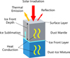 |
Fig. 1 Schematic of the dust-mantle model. |
Parameters of saturation vapor pressure and sublimation latent heat (Huebner et al. 2006).
2.1.2 Nongravitational force
The sublimation of volatiles on the surface of the nucleus generates a reactive force. According to the conservation of momentum, the recoil force on a single surface facet can be expressed as
 (9)
(9)
where η is the momentum transfer coefficient, which was set to 0.6 in this study according to Attree et al. (2019). Sk represents the area of the k-th facet in the shape model described in Sect. 2.1.4, Vgas is the gas velocity, and nk is the unit normal vector of the facet. The sublimation rate ω (Tk) can be calculated using Eq. (6). The gas velocity can be determined from the average velocity in the Maxwell-Boltzmann distribution:
 (10)
(10)
The total recoil torque acting on the cometary nucleus is given by
 (11)
(11)
where rk is the vector from the nucleus’s center of mass to the facet. During the calculation, rk, Fk, and M were projected onto the comet’s principal-axis frame to facilitate the solution of the attitude-dynamics equations described in Sect. 3.1.
2.1.3 Numerical procedure
The subsurface domain above a prescribed ice-front depth Z is discretized into layers of thickness Δx. At each time step Δtth (where th denotes the thermophysical model), the procedure is as follows: first, a Newton-Raphson iteration solves for the surface temperature and the ice-front temperature that satisfy the boundary conditions (Eqs. (2) and (3)); then, the heat-conduction partial differential equation (Eq. (1)) is advanced in time using the Crank-Nicolson scheme (Hu 2017).
Numerical stability of the Crank-Nicolson method requires
 (12)
(12)
In the uniform grid setting, the ice-front depth D is constrained to be an integer multiple of the depth step Δx. During the inversion procedure, D was treated as a free parameter that must vary continuously from the surface down to several centimeters. This requirement can be accommodated by reducing Δx; however, when D is small (e.g., D = 1 mm), the stability criterion forces both Δx and the corresponding time step Δtth to become very small (e.g., Δtth ≤ 18 s), leading to prohibitively high computational costs while offering little improvement in the accuracy of recoil force estimation.
To overcome this limitation, we constructed a neural-network surrogate for the full thermophysical model. The high-fidelity thermophysical model was used to generate training data with Δx = 2 mm and Δtth = 60 s, which strikes a balance between accuracy and efficiency. The surrogate can then predict sublimation-induced recoil forces at arbitrary, larger time steps without being restricted by the Δtth – Δx stability condition, thereby greatly enhancing computational efficiency.
2.1.4 Model parameterization
Table 2 lists the parameters used in the thermal simulation. In this study, the ice-front depth is a variable parameter, with its value determined through attitude fitting as described in Sect. 4. Due to insufficient observational data, the thermal parameters of the dust mantle and dust-ice mixture were assumed to be equal. Table 2 provides the values for the density, specific heat, and thermal inertia, while the thermal conductivity is calculated using the following equation:
 (13)
(13)
Groussin et al. (2013) analyzed infrared spectral images obtained by EPOXI and found that the thermal inertia of 103P’s nucleus is less than 250 W · (K m2 s1/2)−1. The value of thermal inertia affects the magnitude of the ice-front depth obtained by inversion, but it does not significantly impact the overall depth distribution of the nucleus. This study adopted the thermal inertia value used in the thermal modeling of 103P by Yue et al. (2023).
The volatile area coverage fraction parea has little effect on the thermal simulation results. By assuming near-surface sublimation and neglecting heat conduction, the energy input from solar irradiation equals the thermal radiation and sublimation heat absorption. As parea decreases, the surface temperature must rise to satisfy energy conservation. Since the temperature gradient for heat absorption of sublimation is greater than the temperature gradient for thermal radiation, the energy deficit caused by the reduction in parea is mainly made up by the increased sublimation rate. The total heat absorption of sublimation can be approximated as a constant, meaning the total sublimation rate does not change significantly with parea. In this study, the area coverage fractions for H2O and CO2 were set to 0.397 according to Yue et al. (2023).
This study used the 103P shape model from the NASA Planetary Data System (Farnham & Thomas 2013). The model consists of 32 040 facets and 16 022 vertices, with vertices uniformly distributed by latitude and longitude at a 2° step size. Using this model directly would result in excessive computation time. Therefore, the model was simplified by adjusting the latitude step size to 2–6° and the longitude step size to 30° (with grid refinement near the small end of the nucleus to accommodate larger variations in the comet-centric distance). The simplified model consists of 1640 facets. In this study, the ice-front depth in the thermal model was treated as a free parameter. However, assigning an individual parameter to each surface facet would result in over-parameterization and reduce the robustness of the results. To address this, a localized activity model (see Sect. 4.2) was developed to describe the spatial distribution of ice-front depth across the nucleus surface. This approach reduces the number of free parameters in the model to 11.
2.2 Neural-network surrogate
The computational expense of the full thermophysical simulation – driven by stringent Δtth – Δx stability constraints –renders direct use of the model impractical for parameter estimation. To overcome this, we employed a neural-network surrogate. Sect. 2.2.1 describes the network architecture, Sect. 2.2.2 details the training and testing datasets, and Sect. 2.2.3 evaluates the surrogate’s performance.
2.2.1 Neural network architecture
A straightforward surrogate would map the state variables across each subsurface layer from one time step to the next. However, this approach entails a high-dimensional, multi-output network that is difficult to train and complicated by varying discretizations across different ice-front depths. Because our primary interest is the sublimation-driven recoil force, which directly governs the NGT, we instead configured the network to predict this single scalar output. To capture the model’s dependence on prior boundary conditions, we included the historical solar irra-diance over a fixed time window Ts as an input. Additionally, since the ice-front depth was treated as a free parameter in the attitude inversion, it was also provided as an input feature.
The resulting architecture (Fig. 2) consists of fully connected layers (FC layers) with tanh activations and residual connections (He et al. 2016) to mitigate vanishing gradients in deep networks. Solar irradiance and ice-front depth each pass through two residual blocks; their processed representations were then concatenated and fed into two further residual blocks, culminating in the recoil-force output.
In our implementation, the solar-irradiance input was set to a 289-dimensional vector sampling the past Ts = 24 h at ΔTs = 5 min intervals (including the current time point), while the ice-front depth and the predicted recoil force were set to one-dimensional scalars. The choice of Ts and ΔTs reflects a trade-off between accuracy and computational efficiency.
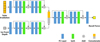 |
Fig. 2 Neural network architecture. |
Neural network test results.
2.2.2 Dataset construction
This study used the thermal model described in Sect. 2.1 to generate training and testing datasets for H2O and CO2, respectively, through nucleus free rotation simulations. The simulation time spanned the period covered by the attitude variation data introduced in Sect. 4. For both H2O and CO2, the ice-front depths covered the depth range from the surface to 70 mm and 250 mm, respectively. To construct the dataset, 90% of the facets from the nucleus shape model were randomly selected to generate the training set, while the remaining 10% were reserved for the testing set.
For data normalization, Min-Max normalization was applied to both the solar irradiation and ice-front depth. Since recoil forces at different depths follow a long-tail distribution, the output recoil force was logarithmically normalized as follows:
 (14)
(14)
where F is the sublimation recoil force, Fmax is the maximum recoil force (set to 0.1 N/m2), and FN is the normalized output.
2.2.3 Network evaluation
Using the dataset described in Sect. 2.2.2, we trained and tested separate surrogates for H2O and CO2. All code was written in MATLAB R2023b and run on an Intel Core i7-14700 processor. Table 3 summarizes the H2O network’s performance on the testing set for single-step thermophysical simulations, while Fig. 3 compares the network’s predictions against the full thermal model across a range of ice-front depths. The surrogate maintains high accuracy at all depths and delivers approximately a tenfold speedup over the original physical model for single-step runs. Moreover, since it is not subject to the Crank-Nicolson stability constraint, recoil forces can be sampled at arbitrary intervals. In this study, we adopted a sampling interval Δtnn = 600 s (where nn denotes the neural network) to balance efficiency and accuracy, and interpolated between these points to reconstruct the torque time series.
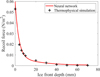 |
Fig. 3 Comparison of recoil force calculation between neural-network surrogate and thermophysical simulation. |
3 Coupled attitude-thermal simulation
To accurately simulate the rotational motion of the cometary nucleus, we employed the Euler equations for rigid-body rotation, as introduced in Sect. 3.1. The thermal and attitude-dynamics models are coupled through the sublimation recoil torque, and the overall coupled attitude-thermal simulation process is described in Sect. 3.2.
3.1 Attitude-dynamics model
We formulated the rotational dynamics of the nucleus using Euler’s equations, expressed as a system of ordinary differential equations (ODEs) in terms of the Euler angles Φ, Θ, Ψ, and the angular velocity vector ω. Readers may refer to Goldstein (2011) for a detailed derivation. Similar modeling approaches have been applied to comet 1P/Halley (Julian 1990; Samarasinha & Belton 1995).
The nucleus’s attitude is described using Euler angles following a 3–2–1 rotation sequence, which transforms from the inertial frame to the principal-axis frame: a rotation by Ψ about the inertial z-axis, followed by Θ about the intermediate y-axis, and finally Φ about the final x-axis. The time derivatives of the Euler angles in the principal-axis frame are given by
![Mathematical equation: $\left[ {\matrix{ {\mathop \Phi \limits^\cdot } \cr {\mathop \Theta \limits^\cdot } \cr {\mathop \Psi \limits^\cdot } \cr } } \right] = \left[ {\matrix{ 1 & {\sin \left( \Phi \right)\tan \Theta } & {\cos \left( \Phi \right)\tan \Theta } \cr 0 & {\cos \left( \Phi \right)} & { - \sin \left( \Phi \right)} \cr 0 & {\sin \left( \Phi \right)\sec \left( \Theta \right)} & {\cos \left( \Phi \right)\sec \left( \Theta \right)} \cr } } \right]\omega ,$](/articles/aa/full_html/2025/11/aa54487-25/aa54487-25-eq15.png) (15)
(15)
where ω is the angular velocity vector in the principal-axis frame. This formulation encounters singularities when  due to the tan Θ and sec Θ terms. In our numerical simulations, we addressed this issue using smooth interpolation near the singularities.
The rotational dynamics in the principal-axis frame are governed by Euler’s equations:
 (16)
(16)
where I = diag(Ix, Iy, Iz) is the inertia matrix. Together with the Euler angle kinematics, this system forms a complete set of ODEs. To solve it, initial conditions must be specified. In this study, we adopted the spin-state parameters for 103P at the closest approach epoch as determined by Belton et al. (2013), as listed in Table 4. All quantities – including moments of inertia, angular momentum, rotational energy, and torque – are expressed per unit mass. The angular momentum direction provided by Belton et al. (2013) relates to the angular velocity via
 (17)
(17)
The recoil torque M in the equation above was obtained from the sublimation force model described in Eqs. (9) and (11). Consequently, the ODE system must be solved in tandem with the thermal simulation, as described in Sect. 3.2.
3.2 Simulation process
The nucleus’s rotational dynamics and its thermophysical evolution are coupled through Eqs. (11) and (16) and therefore must be integrated simultaneously. In this work, we used the neural-network surrogate developed in Sect. 2.2 together with the rigid body attitude model from Sect. 3.1 to perform a coupled simulation.
Because the attitude integration time step Δtatt (where att denotes the attitude-dynamics model, typically on the order of tens of seconds) is much shorter than the surrogate sampling interval (Δtnn = 600 s, introduced in Sect. 2.2.3), evaluating the sublimation recoil torque at every attitude step would be computationally prohibitive. To mitigate this, we decoupled the two processes over each sampling interval by assuming that, within Δtnn, the effect of the recoil torque on the attitude is negligible. Thus, each simulation interval proceeds in three stages:
Free rotation: integrate the attitude ODEs over [t, t + Δtnn] without any torque to estimate the attitude trajectory.
Torque computation: from that trajectory, compute the surface irradiance over [t, t + Δtnn]. Combine these values with the previous irradiance history over [t – Ts, t]. The neural-network surrogate requires this history because subsurface heat conduction and latent heat storage introduce a delayed thermal response that depends on past insolation (see Sect. 2.2). Input both into the surrogate to predict the sublimation recoil-torque time series across the interval.
Forced rotation: reintegrate the attitude ODEs over [t, t + Δtnn] including the interpolated torque to update the rotational state.
Since our initial spin state was defined at closest approach – and the observational data span many days both before and after that moment – we performed both forward and backward integrations: for the forward simulation, the past irradiance record over [t – Ts, t] is known a priori. We applied the three-stage procedure above at each step to march from the encounter epoch outward. For the backward simulation, the irradiance history is not known. At each backward step t → t – Δtnn, we first performed a free rotation integration over [t – Δtnn – Ts, t] to reconstruct the attitude and thus infer irradiance over [t – Δtnn – Ts, t – Δtnn]. We then used the surrogate to compute the torque on [t – Δtnn, t] and performed a forced rotation integration backward over that same interval. Repeating this process recovers the pre-encounter rotational evolution.
A schematic of the entire coupled workflow is shown in Fig. 4. This approach ensures accurate tracking of the comet’s attitude under time-varying sublimation torques while maintaining computational efficiency.
Parameters of the attitude-dynamics model (Belton et al. 2013).
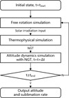 |
Fig. 4 Coupled attitude-thermal simulation process. |
4 Ice-front depth inversion
Based on the coupled attitude-thermal simulation model and thermal surrogate model, this study utilized attitude variation data and volatile production rate data obtained from the EPOXI mission to invert the ice-front depths of different volatiles on the nucleus surface. Sect. 4.1 introduces the fitting data used, Sect. 4.2 describes the ice-front depth inversion model, Sect. 4.3 presents the objective function of the optimization problem, and Sect. 4.4 outlines the solution procedure.
4.1 Fitting data
This study used attitude variation data and CO2 production rate data as fitting data to invert the ice-front depths for different regions of the cometary nucleus. The attitude variation data was sourced from Belton et al. (2013). Belton estimated the spin and precession periods of 103P’s long axis using EPOXI and radar observation data, and further calculated the changes in the comet’s angular momentum and rotational energy, as shown in Table 5.
CO2 production rate data was sourced from A’Hearn et al. (2011). By analyzing the spectral images at closest approach, A’Hearn estimated the average production rates of H2O and CO2 are  mole/s and
  mole/s, respectively.
4.2 Ice-front depth inversion model
According to the EPOXI observations, the distribution of volatiles on the surface of 103P shows significant inhomogeneity (A’Hearn et al. 2011). CO2 primarily sublimates from the small end of the nucleus, while H2O shows stronger activity at the waist of the nucleus. Additionally, the waist exhibits a smoother surface than other regions, and A’Hearn suggested that the materials in this region may originate from a settling mechanism.
Based on these observations, 103P nucleus was divided into three regions: the large end, the waist, and the small end, using –6° and 60° latitudes in the principal-axis frame. CO2 sublimation was considered for the large and small ends, while H2O sublimation was considered for the waist.
To further describe the inhomogeneous distribution of surface materials, this study introduced a localized activity model. In this model, the nucleus surface was divided into uniformly sublimating regions and several localized activity regions. The localized activity regions are illustrated in Fig. 5, where the ice-front depth follows a specific distribution within a certain radius Ri from the center of activity Ai. The position of activity center Ai is expressed in terms of latitude λi and longitude φi in the principal-axis frame.
Within the active regions, this study used a quadratic function to model the ice-front depth distribution, as shown in Fig. 6. The ice-front depth D at a distance Δ from the center of activity follows the relation:
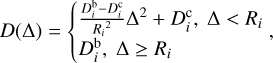 (18)
(18)
where  is the ice-front depth at the center of the active region, and
  is the background ice-front depth. In Eqs. (18) and (19), we set i = 0 for the waist, i = 1 for the large end, and i = 2 for the small end.
The inversion problem was formulated as an optimization problem. Assuming uniform sublimation of H2O at the waist with an ice-front depth of  , and setting localized activity regions for CO2 at the large end (i = 1) and small end (i = 2), the optimization variables can be expressed as
![Mathematical equation: $y = {\left[ {D_0^{\rm{b}}\,\,D_1^{\rm{b}}\,\,D_1^{\rm{c}}\,\,{\lambda _1}\,\,{\varphi _1}\,\,{R_1}\,\,D_2^{\rm{b}}\,\,D_2^{\rm{c}}\,\,{\lambda _2}\,\,{\varphi _2}\,\,{R_2}} \right]^{\rm{T}}}.$](/articles/aa/full_html/2025/11/aa54487-25/aa54487-25-eq25.png) (19)
(19)
Variations in the angular momentum and rotational energy of 103P throughout the encounter (Belton et al. 2013).
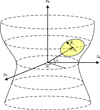 |
Fig. 5 Schematic of the localized activity model. The axes xb, yb, and zb define the principal-axis frame, aligned with the minimum, intermediate, and maximum principal inertia axes, respectively. |
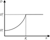 |
Fig. 6 Schematic of ice-front depth distribution. |
4.3 Objective function
In this study, the variations in angular momentum and rotational energy were used for parameter fitting. The objective function of the optimization problem was formulated as a weighted least squares expression:
 (20)
(20)
where ti, Hi, and Ei represent the i-th time point, angular momentum, and rotational energy observation, respectively, as listed in Table 5.  and
and  denote the associated uncertainties of angular momentum and rotational energy. The modeled angular momentum and rotational energy at time ti can be calculated as
 (21)
(21)
 (22)
(22)
For volatile production rate observations, the hyperactivity of 103P must be taken into account. A significant portion of the H2O production may result from the sublimation of ice grains ejected by CO2-driven activity, rather than from direct surface sublimation. In addition, the CO2 production rate data may carry considerable uncertainty. Therefore, in this study, the CO2 production rate was used solely as a constraint rather than as a direct fitting target:
 (23)
(23)
where  is the relaxation coefficient, which was taken as 0.3, and
  is the simulated CO2 production rate averaged over one spin period:
 (24)
(24)
where to is observation instant, Tr is the spin period, taken as the precession period of 18.4 h, and  corresponds to the surface region of CO2.
4.4 Inversion procedure
In our implementation, the constraint (23) was incorporated into the objective function using a penalty function. The optimization problem for retrieving the ice-front depth can be expressed as
 (25)
(25)
where the parameter ξ determines the penalty strength, and the function max (·) denotes the maximum operator.
This optimization problem is strongly nonlinear, and gradient-based optimization algorithms tend to be trapped in local minima. Therefore, in this work, we adopted the particle swarm optimization (PSO) algorithm, which is a global optimization method. PSO conducts a population-based search, where each particle is characterized by its position (i.e., the values of the optimization variables) and its velocity (the difference of the optimization variables between two successive iterations). At each iteration, PSO evaluates the objective function for all particles and updates their positions and velocities according to a specific strategy. For more details on PSO, the reader is referred to Kennedy & Eberhart (1995).
The time complexity of PSO can be expressed as O (Np Ni CJ) where Np is the number of particles, Ni is the number of iterations, and CJ is the computational cost of a single objective function evaluation. In each iteration, the particle parameters were substituted into the localized activity model to compute the ice-front depth of all surface facets of the nucleus, followed by a coupled attitude-thermal simulation to obtain the attitude evolution and volatile production rates. In this process, the time complexity is primarily dominated by the attitude integration and the thermophysical model.
For the attitude dynamics, the Runge–Kutta method was used to integrate the differential equations, with a time complexity of O (tsimu / Δtatt ), where tsimu denotes the total simulation duration. The thermophysical model primarily involves solving a one-dimensional nonlinear heat conduction equation and a tridiagonal linear system. The Newton-Raphson iteration used for the nonlinear equation scales as O (log log (1/ε)), where ε is the convergence tolerance, while the Thomas algorithm for the tridiagonal system scales as O (nt), with nt being the number of layers. Therefore, the overall time complexity of the thermophysical model can be expressed as O (tsimu/Δtth · (log log (1/ε) + nt)). When a neural-network surrogate is employed for computing the recoil torque, the complexity becomes  , where L is the number of layers and nl the dimension of the l-th layer. On a per-step basis, the neural network does not provide a dramatic time-complexity advantage over the full thermophysical model. Its real benefit lies in the absence of numerical-stability constraints on the time step, which allows for the use of much larger time steps while maintaining sufficient accuracy. This significantly reduces the computational cost of the coupled simulation.
5 Results and discussion
5.1 Inversion results
The optimal value of the objective function obtained from solving the optimization problem constructed in Sect. 4 is 65.45. The variations in angular momentum and rotational energy are shown in Fig. 7. The simulated angular momentum and rotational energy exhibit superposed short-term oscillations and a long-term linear decay, in excellent agreement with the estimates of Belton et al. (2013).
The inversion results for the optimization variables are shown in Table 6. The resulting ice-front depth distribution on the nucleus surface, calculated using the parameters from Table 6, is shown in Fig. 8. The results show that the ice-front depth of H2O is on the millimeter scale, while CO2 ice-front depths are concentrated in the centimeter to decimeter range. At the center of the active region, CO2 sublimates close to the surface. The active center of the small end lies along the nucleus’s long axis, while the active center of the large end is located on the side of the nucleus. Although the small end exhibits intense sublimation rates at the observation instant, the inversion results indicate that the large end is more active, exhibiting a shallower ice-front depth distribution.
It should be noted that, because our model cannot fully capture all the physical processes of the nucleus, the fitted parameters carry significant uncertainties. For instance, the thermal inertia strongly influences the absolute ice-front depths, yet its true value is poorly constrained. Groussin et al. (2013) estimated a thermal inertia below 250 W (K m2 s1/2)−1 via photometric methods; we adopted a value of 50 W (K m2 s1/2)−1, as used by Yue et al. (2023) in their study of 103P. In our recoil-force model, we assumed a Maxwell-Boltzmann velocity distribution and characterize deviations from the thermal speed using a momentum-transfer coefficient fitted by Attree et al. (2019), which likewise introduces uncertainty. Furthermore, owing to the limited observational dataset, we modeled only two localized sources at the nucleus’s ends, even though the EPOXI observations revealed multiple distinct jets (Protopapa et al. 2014).
Despite these uncertainties, any systematic biases are likely uniform across the nucleus, so the overall volatile-distribution pattern remains a useful reference. The close match between our simulated sublimation rates and the observations (see Sect. 5.2) further supports the validity of our inversion results.
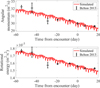 |
Fig. 7 Variations in angular momentum and rotational energy. The upper graph shows the angular momentum variation, and the lower graph shows the rotational energy variation. The black crosses represent Belton’s estimates (Belton et al. 2013), and the red curve represents the fitting results from this study. |
Inversion results.
 |
Fig. 8 Ice-front depth distribution on the nucleus surface. CO2 ice-front depth is shown for the large and small ends, and H2O ice-front depth is shown for the waist of the nucleus. The nucleus’s attitude and observation direction are set to E+7 minutes to align with the EPOXI observation data. The left graph shows the front side distribution, and the right graph shows the reverse side distribution. The temperature-time variation for facet A on the large end, and the temperature-depth distribution for facet B on the small end, are analyzed further in Figs. 10 and 11, respectively. |
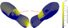 |
Fig. 9 Distribution of volatile sublimation rates on the nucleus surface. The sublimation rate of CO2 is displayed for the end regions, while the sublimation rate of H2O is shown for the waist region. The nucleus’s attitude and observation direction are set to E+7 minutes to align with EPOXI observation data. The left graph shows the front side distribution, and the right graph shows the reverse side distribution. The red line indicates the solar direction. |
5.2 Volatile distribution analysis
Based on the results in Fig. 8, we further calculated the sublimation rate distribution at E+7 minutes and compared it with the near-field observation data from EPOXI. The sublimation rate distributions for CO2 and H2O are shown in Fig. 9. Our fitting results are in high agreement with the calculations from A’Hearn et al. (2011) and Protopapa et al. (2014). H2O sublimates from the waist of the cometary nucleus, while CO2 primarily sublimates from the sunlit small end of the nucleus. Although there is no direct solar irradiation input at the large end of the nucleus, sublimation is still observed in this region, with the ice-front depth approximately 80 mm. At this depth, the heat flux from above is sufficient to support CO2 sublimation, and the overlying dust mantle provides insulation, causing this region to sublimated at a stable rate over the spin cycle. The temperature variations are shown in Fig. 10. In general, the CO2 sublimation rate distribution is correlated with the J1, J3, and J4 jets annotated by Protopapa et al. (2014).
For volatile production rates, the simulated average CO2 production rate near E-55 hours is 1.91 × 1027 mole/s, which is close to the result from A’Hearn et al. (2011) (2.0 × 1027 mole/s). In our model, the large end has a shallower ice-front depth and a larger active region, making it easier for CO2 to sublimate. As a result, the large end contributes 74% of the total CO2 production rate, while the small end contributes 26%. Despite the fact that solar radiation directly hits the small end rather than the large end at the observation instant, the significant outflows from the large end indicate its highly activity. The average H2O production rate at the waist is only 7.68 × 1026 mole/s, much lower than the observed value (1.0 × 1028 mole/s). The total H2O production rate for 103P likely originates mainly from the water ice ejected by CO2 sublimation at the nucleus’s ends, a result consistent with Belton et al. (2013).
Based on the observations, although CO2 from the small end carries water ice, no significant water vapor distribution is observed at the small end, indicating that the H2O ice-front temperature at the small end is below the sublimation temperature. Fig. 11 shows the temperature distribution for a facet at the small end. The ice-front depth for CO2 is about 30 mm, and it can be inferred that the H2O ice-front depth at this facet is between 20 and 30 mm.
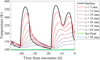 |
Fig. 10 Temporal temperature variation for facet A on the large end. The location of the facet is marked in Fig. 8, and the ice-front depth at this facet is 80 mm. The presence of the dust mantle above keeps the temperature of the ice front stable throughout the entire spin cycle. |
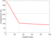 |
Fig. 11 Temperature-depth profile for facet B on the small end. The location of the facet is marked in Fig. 8, with the CO2 ice-front depth at this facet at 30 mm. The black horizontal line indicates the sublimation temperature of water ice, and the blue vertical line shows the CO2 icefront depth at this facet. |
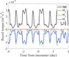 |
Fig. 12 Variation of sublimation recoil torque during the encounter. The torque is projected onto the principal-axis frame. The black curve represents the magnitude of the torque, and the red, green, and blue curves represent the torque components along the x-axis (minimum inertia axis), y-axis (intermediate inertia axis), and z-axis (maximum inertia axis), respectively. |
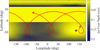 |
Fig. 13 Trajectory of the sub-solar point from E-2 days to the encounter epoch. The red pentagram marks the moment of encounter, the red triangle marks the subsolar point two days before, and the blue cross indicates the location of the active center on the large end. The latitude range –90° to –6° defines the large end, –6° to 60° the waist, and 60° to 90° the small end. |
5.3 Rotation analysis
Fig. 12 shows the evolution of the sublimation-driven recoil torque on 103P’s nucleus during the encounter. The bulk of the torque is concentrated along the principal-axis y and z directions, with only a minor component about the minimal-inertia x-axis. Because the comet’s perihelion distance varied little (1.1–1.2 AU), the peak recoil torque remained essentially constant at 3 × 10⁻⁵ m2 /s2, with a mean value of 1 × 10⁻⁵ m2 /s2. Scaling by the nucleus mass of 2.4 × 10¹¹ kg yields a torque of 3 × 10⁶ kg m2/s2, exceeding the 9.5 × 10⁴ kg m2/s2 estimate of Belton et al. (2013). The discrepancy arises because Belton et al. assumed the torque always acts parallel to the angular-momentum vector – maximizing its efficiency – whereas in our model the torque vector rotates with the body frame, altering both the magnitude and direction of H.
In the two days leading up to the EPOXI encounter, the sub-solar point on the nucleus traces the paths shown in Figs. 13 and 14. It spends approximately equal time in both hemispheres, but exhibits distinctly different behaviors: when crossing the northern hemisphere, the sub solar point moves rapidly across a broad range of longitudes, whereas in the southern hemisphere it follows a more persistent, droplet shaped loop over a localized region, maintaining prolonged insolation. In the hours immediately before encounter, the sub solar point dwells between 0° and 30° longitude, delivering concentrated heat to this sector. This focused illumination explains the CO2 sublimation observed on the shadowed side of the large end at approximately 50° longitude, seven minutes after closest approach.
Fig. 14 plots the instantaneous recoil-torque contributions from the large end, waist, and small end over the same interval. Because the large-end activity center is offset from the comet’s center of mass, its recoil force produces an eccentric moment that depends primarily on sub-solar longitude. Consequently, the large end generates over 90 % of the net sublimation torque during the encounter. By contrast, H2O and CO2 outgassing at the waist and small end is distributed more uniformly in longitude; their torques are therefore modulated mainly by sub-solar latitude and average out to a small net value over one rotation.
Fig. 15 shows the time history of the excitation index k2, defined following Samarasinha & A’Hearn (1991) as a negative correlation measure of long-axis excitation:
 (26)
(26)
In this formulation, k2 < 1 corresponds to the excited long-axis mode (LAM), in which the nucleus rotates about its long axis while nutating about the short axes; k2 > 1 corresponds to the short-axis mode, with rotation about the short axis and oscillation about the long axes. Because the angular momentum and rotational energy decay nearly linearly during the encounter, k2 rises gradually before perihelion and then drops sharply afterward, indicating an increase in long-axis excitation. If 103P maintains its current activity pattern, we anticipate further enhancement of LAM excitation, eventually transitioning toward principal-axis rotation. Under continued perihelion passages, the spin rate should increase incrementally, ultimately reaching the breakup threshold and causing nucleus fragmentation.
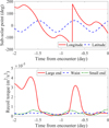 |
Fig. 14 Time evolution of the sub-solar point coordinates and the sublimation-driven recoil torques ||M|| over the two days preceding closest approach. Top panel: sub-solar longitude and latitude as functions of time. Bottom panel: torque contributions from the large end, waist, and small end of the nucleus. |
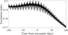 |
Fig. 15 Evolution of the excitation index, as defined by Eq. (26), over ±100 days around the encounter. |
6 Conclusion
We developed a coupled attitude-thermal model for comet 103P, leveraging a neural-network surrogate to accelerate the thermo-physical simulations. By fitting the nucleus’s rotational-variation data, we successfully constrained the spatial distributions for H2O and CO2. The main conclusions of this study are as follows:
Guided by observational constraints, we partitioned the nucleus into three zones – large end, waist, and small end – and assigned CO2 sublimation to the two ends and H2O sublimation to the waist. Our model accurately reproduces the comet’s attitude changes and volatile output during the encounter. The simulated angular momentum and rotational energy exhibit superposed short-term oscillations and a long-term linear decay, in excellent agreement with Belton et al. (2013). At E+7 minutes, H2O outgassing predominates at the waist, while CO2 sublimation peaks on the sunlit small end and persists beneath the dusty mantle at the shadowed large end, matching spacecraft observations;
We find that the CO2 ice front at both ends lies between centimeters and decimeters, whereas the H2O ice front at the waist is only millimeters deep. The large end exhibits stronger CO2 activity than the small end. At the time of observation, the dust mantle over the large end insulates the subsurface CO2, allowing continued outgassing in shadowed regions. The fitted average CO2 production rate is 1.91 × 1027 mole/s – very close to the measured value – while the waist’s H2O production rate is 7.69 × 1026 mole/s, only about 8% of the observed total. This implies that most of the H2O production likely originates from water ice grains ejected by CO2 jets at the nucleus’s ends. From the modeled temperature profile, we estimate the H2O ice-front depth at the ends to be 20–30 mm;
The large end’s CO2 source, being offset from the nucleus’s center of mass, generates over 90% of the net recoil torque, and thus dominates the rotational dynamics. In the hours leading up to the encounter, this region remained continuously illuminated, allowing CO2 to sublimate even on the shadowed side at the moment of observation. The excitation index shows a transient increase in LAM excitation after perihelion. If the present activity pattern persists, we anticipate further growth in long-axis excitation and an eventual transition toward principal-axis rotation.
Despite these advances, our study has some limitations. In the current thermal model, the ice-front depth was treated as a constant, even though it likely evolves with heliocentric distance (Marboeuf et al. 2012). In future work, we intend to introduce a thermal evolution model to explore how the ice-front depth varies over the comet’s orbit.
Acknowledgements
We gratefully acknowledge the anonymous reviewer for the constructive comments, which have substantially improved this manuscript. We also thank the many engineers and scientists whose dedicated efforts were critical to obtaining data on comet 103P/Hartley 2. This work was supported by the Beijing Natural Science Foundation (Grant No. L248032) and the National Natural Science Foundation of China (Grant No. 41804165).
References
- A’Hearn, M. F., Belton, M. J. S., Delamere, W. A., et al. 2011, Science, 332, 1396 [CrossRef] [Google Scholar]
- Attree, N., Jorda, L., Groussin, O., et al. 2019, A&A, 630, A18 [NASA ADS] [CrossRef] [EDP Sciences] [Google Scholar]
- Attree, N., Jorda, L., Groussin, O., et al. 2023, A&A, 670, A170 [NASA ADS] [CrossRef] [EDP Sciences] [Google Scholar]
- Attree, N., Gutiérrez, P., Groussin, O., et al. 2024, A&A, 690, A82 [NASA ADS] [CrossRef] [EDP Sciences] [Google Scholar]
- Belton, M. J. S., Thomas, P., Li, J.-Y., et al. 2013, Icarus, 222, 595 [Google Scholar]
- Bockelée-Morvan, D., Crovisier, J., Mumma, M. J., & Weaver, H. A. 2004, Comets II, 1, 391 [Google Scholar]
- Bürger, J., Hayne, P. O., Gundlach, B., et al. 2024, JGR Planets, 129, e2023JE008152 [Google Scholar]
- Davidsson, B. J. 2021, MNRAS, 505, 5654 [NASA ADS] [CrossRef] [Google Scholar]
- Davidsson, B. J., Samarasinha, N. H., Farnocchia, D., & Gutiérrez, P. J. 2022, MNRAS, 509, 3065 [Google Scholar]
- Encke, J. 1821, B.A.J., 1824, 216 [Google Scholar]
- Farnham, T., & Thomas, P. 2013, Plate shape model of comet 103P/Hartley 2 V1.0, Dif-C-Hriv/Mri-5-Hartley2-Shape-V1.0 [Google Scholar]
- Filacchione, G., De Sanctis, M. C., Capaccioni, F., et al. 2016, Nature, 529, 368 [NASA ADS] [CrossRef] [Google Scholar]
- Giorgini, J. D., & Group, J. S. S. D. 2025, NASA/JPL Horizons OnLine Ephemeris System, https://ssd.jpl.nasa.gov/horizons/, data retrieved 2025-06-06 [Google Scholar]
- Goldstein, H. 2011, Classical Mechanics (Pearson) [Google Scholar]
- Groussin, O., Lamy, P., Jorda, L., & Toth, I. 2004, A&A, 419, 375 [NASA ADS] [CrossRef] [EDP Sciences] [Google Scholar]
- Groussin, O., Sunshine, J. M., Feaga, L. M., et al. 2013, Icarus, 222, 580 [CrossRef] [Google Scholar]
- Groussin, O., Attree, N., Brouet, Y., et al. 2019, Space Sci. Rev., 215, 29 [Google Scholar]
- Gutiérrez, P. J., Ortiz, J. L., Rodrigo, R., López-Moreno, J. J., & Jorda, L. 2002, Earth Moon Planets, 90, 239 [Google Scholar]
- He, K., Zhang, X., Ren, S., & Sun, J. 2016, in Proceedings of the IEEE Conference on Computer Vision and Pattern Recognition, 770 [Google Scholar]
- Hu, X. 2017, Thesis, Technischen Universität Carolo-Wilhelmina zu Braunschweig, Germany [Google Scholar]
- Hu, X., Shi, X., Sierks, H., et al. 2017, MNRAS, 469, S295 [NASA ADS] [CrossRef] [Google Scholar]
- Huebner, W. F., Benkhoff, J., Capria, M.-T., et al. 2006, Heat and Gas Diffusion in Comet Nuclei, 133 (Bern: International Space Science Institute) [Google Scholar]
- Julian, W. H. 1990, Icarus, 88, 355 [NASA ADS] [CrossRef] [Google Scholar]
- Kennedy, J., & Eberhart, R. 1995, in Proceedings of ICNN’95-International Conference on Neural Networks, 4, IEEE, 1942 [Google Scholar]
- Kührt, E. 1999, Space Sci. Rev., 90, 75 [Google Scholar]
- Lagerros, J. 1996, A&A, 310, 1011 [NASA ADS] [Google Scholar]
- Läuter, M., & Kramer, T. 2025, A&A, 699, A75 [NASA ADS] [CrossRef] [EDP Sciences] [Google Scholar]
- Li, J. Y., Besse, S., A’Hearn, M. F., et al. 2013, Icarus, 222, 559 [CrossRef] [Google Scholar]
- Marboeuf, U., Schmitt, B., Petit, J. M., Mousis, O., & Fray, N. 2012, A&A, 542, A82 [NASA ADS] [CrossRef] [EDP Sciences] [Google Scholar]
- Marschall, R., Davidsson, B. J., Rubin, M., & Tenishev, V. 2024, Comets III, 433 [Google Scholar]
- Marsden, B. G. 1969, AJ, 74, 720 [Google Scholar]
- Marsden, B. G. 2009, P&SS, 57, 1098 [Google Scholar]
- Marsden, B. G., Sekanina, Z., & Yeomans, D. K. 1973, AJ, 78, 211 [NASA ADS] [CrossRef] [Google Scholar]
- Mottola, S., Attree, N., Jorda, L., et al. 2020, Space Sci. Rev., 216, 20 [NASA ADS] [CrossRef] [Google Scholar]
- Mueller, B. E., & Ferrin, I. 1996, Icarus, 123, 463 [Google Scholar]
- Protopapa, S., Sunshine, J. M., Feaga, L. M., et al. 2014, Icarus, 238, 191 [NASA ADS] [CrossRef] [Google Scholar]
- Rickman, H. 1989, Adv. Space Res., 9, 59 [NASA ADS] [CrossRef] [Google Scholar]
- Rickman, H., Kamel, L., Froeschle, C., & Festou, M. 1991, AJ, 102, 1446 [Google Scholar]
- Samarasinha, N. H., & A’Hearn, M. F. 1991, Icarus, 93, 194 [Google Scholar]
- Samarasinha, N. H., & Belton, M. J. 1995, Icarus, 116, 340 [Google Scholar]
- Taylor, A. G., Farnocchia, D., Vokrouhlicky, D., et al. 2024, Icarus, 408, 13 [Google Scholar]
- Weissman, P. R., & Kieffer, H. H. 1981, Icarus, 47, 302 [Google Scholar]
- Yue, Y. X., Liu, J. C., & Wang, X. H. 2023, JGR Planets, 128, 18 [Google Scholar]
All Tables
Parameters of saturation vapor pressure and sublimation latent heat (Huebner et al. 2006).
Variations in the angular momentum and rotational energy of 103P throughout the encounter (Belton et al. 2013).
All Figures
|
Fig. 1 Schematic of the dust-mantle model. |
| In the text | |
|
Fig. 2 Neural network architecture. |
| In the text | |
|
Fig. 3 Comparison of recoil force calculation between neural-network surrogate and thermophysical simulation. |
| In the text | |
|
Fig. 4 Coupled attitude-thermal simulation process. |
| In the text | |
|
Fig. 5 Schematic of the localized activity model. The axes xb, yb, and zb define the principal-axis frame, aligned with the minimum, intermediate, and maximum principal inertia axes, respectively. |
| In the text | |
|
Fig. 6 Schematic of ice-front depth distribution. |
| In the text | |
|
Fig. 7 Variations in angular momentum and rotational energy. The upper graph shows the angular momentum variation, and the lower graph shows the rotational energy variation. The black crosses represent Belton’s estimates (Belton et al. 2013), and the red curve represents the fitting results from this study. |
| In the text | |
|
Fig. 8 Ice-front depth distribution on the nucleus surface. CO2 ice-front depth is shown for the large and small ends, and H2O ice-front depth is shown for the waist of the nucleus. The nucleus’s attitude and observation direction are set to E+7 minutes to align with the EPOXI observation data. The left graph shows the front side distribution, and the right graph shows the reverse side distribution. The temperature-time variation for facet A on the large end, and the temperature-depth distribution for facet B on the small end, are analyzed further in Figs. 10 and 11, respectively. |
| In the text | |
|
Fig. 9 Distribution of volatile sublimation rates on the nucleus surface. The sublimation rate of CO2 is displayed for the end regions, while the sublimation rate of H2O is shown for the waist region. The nucleus’s attitude and observation direction are set to E+7 minutes to align with EPOXI observation data. The left graph shows the front side distribution, and the right graph shows the reverse side distribution. The red line indicates the solar direction. |
| In the text | |
|
Fig. 10 Temporal temperature variation for facet A on the large end. The location of the facet is marked in Fig. 8, and the ice-front depth at this facet is 80 mm. The presence of the dust mantle above keeps the temperature of the ice front stable throughout the entire spin cycle. |
| In the text | |
|
Fig. 11 Temperature-depth profile for facet B on the small end. The location of the facet is marked in Fig. 8, with the CO2 ice-front depth at this facet at 30 mm. The black horizontal line indicates the sublimation temperature of water ice, and the blue vertical line shows the CO2 icefront depth at this facet. |
| In the text | |
|
Fig. 12 Variation of sublimation recoil torque during the encounter. The torque is projected onto the principal-axis frame. The black curve represents the magnitude of the torque, and the red, green, and blue curves represent the torque components along the x-axis (minimum inertia axis), y-axis (intermediate inertia axis), and z-axis (maximum inertia axis), respectively. |
| In the text | |
|
Fig. 13 Trajectory of the sub-solar point from E-2 days to the encounter epoch. The red pentagram marks the moment of encounter, the red triangle marks the subsolar point two days before, and the blue cross indicates the location of the active center on the large end. The latitude range –90° to –6° defines the large end, –6° to 60° the waist, and 60° to 90° the small end. |
| In the text | |
|
Fig. 14 Time evolution of the sub-solar point coordinates and the sublimation-driven recoil torques ||M|| over the two days preceding closest approach. Top panel: sub-solar longitude and latitude as functions of time. Bottom panel: torque contributions from the large end, waist, and small end of the nucleus. |
| In the text | |
|
Fig. 15 Evolution of the excitation index, as defined by Eq. (26), over ±100 days around the encounter. |
| In the text | |
Current usage metrics show cumulative count of Article Views (full-text article views including HTML views, PDF and ePub downloads, according to the available data) and Abstracts Views on Vision4Press platform.
Data correspond to usage on the plateform after 2015. The current usage metrics is available 48-96 hours after online publication and is updated daily on week days.
Initial download of the metrics may take a while.