| Issue |
A&A
Volume 703, November 2025
|
|
|---|---|---|
| Article Number | A163 | |
| Number of page(s) | 23 | |
| Section | Astrophysical processes | |
| DOI | https://doi.org/10.1051/0004-6361/202554871 | |
| Published online | 25 November 2025 | |
Protoplanetary disks around magnetised young stars with large-scale magnetic fields
I. Steady-state solutions
Department of Astrophysics, University of Vienna, Türkenschanzstrasse 17, A-1180 Vienna, Austria
⋆ Corresponding author: This email address is being protected from spambots. You need JavaScript enabled to view it.
Received:
30
March
2025
Accepted:
7
September
2025
Abstract
Context. Describing the large-scale field topology of protoplanetary disks (PPDs) involves significant difficulties and uncertainties. The transport of the large-scale field inside the disk plays an important role in understanding its evolution.
Aims. We aim to improve our understanding of the dependences that stellar magnetic fields pose on the large-scale field. We focus on the innermost disk region (≲0.1 AU), which is crucial for understanding the long-term disk evolution.
Methods. We present a novel approach combining the evolution of a 1+1D hydrodynamic disk with a large-scale magnetic field consisting of a stellar dipole truncating the disk and a fossil field. The magnetic flux transport includes advection and diffusion due to laminar non-ideal magnetohydrodynamic (MHD) effects, such as Ohmic and ambipolar diffusion. Due to the implicit nature of the numerical method, long-term simulations (of the order of several viscous timescales) are feasible.
Results. The large-scale magnetic field topology in stationary models shows a distinct dependence on specific parameters. The innermost disk region is strongly affected by the stellar rotation period and magnetic field strength. The outer disk regions are affected by the X-ray luminosity and the fossil field. Varying the mass flow through the disk affects the large-scale disk field throughout its radial extent.
Conclusions. The topology of the large-scale disk field is affected by several stellar and disk parameters. This will affect the efficiency of MHD outflows, which depend on the magnetic field topology. Such outflows might originate from the very inner disk region, the dead zone, or the outer disk. In subsequent studies, we will use these models as a starting point for conducting long-term evolution simulations of the disk and large-scale field on scales of ∼106 years in order to investigate the combined evolution of the disk, the magnetic field topology, and the resulting MHD outflows.
Key words: accretion, accretion disks / hydrodynamics / protoplanetary disks / stars: formation / stars: magnetic field
© The Authors 2025
 Open Access article, published by EDP Sciences, under the terms of the Creative Commons Attribution License (https://creativecommons.org/licenses/by/4.0), which permits unrestricted use, distribution, and reproduction in any medium, provided the original work is properly cited.
This article is published in open access under the Subscribe to Open model. This email address is being protected from spambots. You need JavaScript enabled to view it. to support open access publication.
1. Introduction
Protoplanetary disks (PPDs) do not evolve in isolation from their environment. Among other parameters, magnetic fields play a crucial role in understanding the evolution of PPDs and can be present in two regions of a disk: (i) strong stellar magnetic fields from the forming protostar, which is most likely partly or fully convective, interacting with the innermost disk, and (ii) large-scale magnetic fields threading the whole disk (e.g. Ohashi et al. 2018; Tang et al. 2023), whose origin is the subject of current research. Either the field is generated inside the disk by some dynamo effect (e.g. Reyes-Ruiz et al. 2004; Brandenburg et al. 1995) or the field is already present during the collapse of the protostellar cloud core (e.g. Dudorov & Khaibrakhmanov 2014). The stellar magnetic field as well as the large-scale disk field strongly influence the dynamics of an evolving PPD on a macroscopic scale (e.g. Ferreira et al. 2006; Bai & Stone 2013; Simon et al. 2013). For instance, angular momentum can be transferred between a protostar and a disk through torques of the stellar field acting on the inner disk parts. The details of such a coupled star-disk system are complex and involve the inclusion of many parameters, for example, the abundance and efficiency of accretion-powered stellar winds (APSW; Gehrig & Vorobyov 2023). Additionally, the position of a magnetically truncated inner disk radius (e.g. Hartmann et al. 2016; Steiner et al. 2021) or the launch of magnetocentrifugal winds (MCWs; Blandford & Payne 1982) are also dependent on the large-scale field. Apart from the macroscopic influence, the development of the magneto-rotational instability (MRI), which in some disk regions is believed to play a non-negligible role in driving accretion (Balbus & Hawley 1991), relies on the abundance of an initial large-scale seed field. The strength of the large-scale field is also believed to be important for determining the efficiency of MRI in PPDs (e.g. Bai & Stone 2011). One approach to investigate how MRI is altered by a magnetic field is to assume a maximally efficient MRI in a steady-state disk, which then determines the magnetic field strength for every radius in the disk (e.g. Mohanty et al. 2018; Delage et al. 2022).
The dipole field strengths of classical T Tauri stars (CTTS) range between 500 G and 1.5 kG (e.g. Johns-Krull et al. 1999; Johnstone et al. 2014) and are therefore strong enough to disrupt the disk at a certain radius, the so-called magnetic truncation radius, rtrunc (Hartmann et al. 2016). Although the details of magnetospheric accretion remain very complex to investigate (e.g. Romanova et al. 2002), it has been shown by Bessolaz et al. (2008) that under the assumption of a dipolar stellar magnetic field, the disk is magnetically truncated very close to the equipartition of magnetic pressure and thermal gas pressure (for detailed simulations of the inner disk movement during disk evolution, e.g. Steiner et al. 2021). Actual observations of large-scale magnetic fields threading a PPD remain challenging; however, magnetic fields have been detected on virtually every observationally accessible scale, including fields abundant in molecular clouds (e.g. Crutcher & Kemball 2019), which indicate that large-scale magnetic fields are likely to be present in a newly forming protostellar core and the resulting PPD. Recent observations of outflows and jets originating from the disk (e.g. Lee 2020) as well as polarisation mapping of the surroundings of T Tauri stars (e.g. Bertrang et al. 2017; Brauer et al. 2017) further strengthen the assumption of large-scale magnetic fields being abundant in PPDs. Additionally, the observation and high-precision measurement of the Zeeman effect in various emission lines has led to the calculation of an upper limit for some PPDs of the order of ∼10 mG for both the poloidal and toroidal fields at r ≈ 40 AU (e.g. Lankhaar & Teague 2023).
The interaction between the disk and the large-scale field is complex. Early 1+1D studies found that an initially purely vertical fossil field threading a thin disk is not dragged inwards efficiently due to outward-directed diffusion counterbalancing inward-directed magnetic advection very easily (e.g. Lubow et al. 1994). Taking the vertical velocity profile of the disk into account has modified this result such that a large-scale field can also be dragged inwards efficiently in a thin disk due to a larger radial mass transport and higher ionisation near the disk surface. The corresponding magnetic resistivity is then adequately averaged in the vertical direction to represent this enhanced magnetic flux transport Guilet & Ogilvie (2012, 2014). However, the source of resistivity is still a subject of investigation. Earlier studies have used turbulent resistivity to describe the non-ideal effects (e.g. Lubow et al. 1994; Guilet & Ogilvie 2012, 2014), but recent studies strongly indicate that PPDs are laminar almost everywhere but the innermost disk region (e.g. Dudorov & Khaibrakhmanov 2014; Mohanty et al. 2018; Delage et al. 2022). Laminar non-ideal diffusion can be caused by Ohmic diffusion (OD), ambipolar diffusion (AD), or the Hall effect (HE).
Apart from 1+1D models, global long-term evolution models have been conducted, including magnetic fields in 2+1D (e.g. Vorobyov et al. 2020). Such models have to deal with the numerical difficulties of conducting magnetohydrodynamic (MHD) simulations over an extended period of time. In particular, the incorporation of magnetic diffusion poses challenges to the numerical stability of a scheme. Furthermore, such models are limited with respect to the position of the inner disk boundary, since the Courant-Friedrichs-Levy (CFL) condition (Courant et al. 1928) severely limits the time step achievable in a disk simulation inside of ∼1 AU. The model of Vorobyov et al. (2020) incorporates large-scale magnetic fields but without considering non-ideal magnetic diffusion due to numerical challenges, which leads to unusually strong magnetic advection and field amplification in their models.
The previous models used to study the influence of a large-scale magnetic field fall short in the following cases: (i) modelling the long-term simulations of a disk and large-scale magnetic field including the inner disk; (ii) modelling the effects of a stellar dipole together with a large-scale field on the inner disk and the topology, especially in the inner disk; (iii) describing the effects of a MCW on the long-term evolution of a PPD. In this work, we aim to investigate the evolution of a large-scale field towards a stationary state for a disk truncated by a stellar dipole. It has been shown that the inner disk treatment is crucial in terms of long-term evolution (e.g. Vorobyov et al. 2019; Steiner et al. 2021; Gehrig et al. 2022). Therefore, a combined treatment of both stellar- and disk components has the potential to alter the disk properties in the inner disk, compared to the common assumption of a torque-free inner disk boundary. A self-consistent evolution of the disk and large-scale magnetic field offers the possibility to study the disk field topology and strength not through assuming maximum efficient MRI (e.g. Mohanty et al. 2018; Delage et al. 2022) but through inward-dragging and amplification of a more physically motivated background fossil field. Furthermore, our simulations are not confined to steady-state models and allowed us to follow the disk field evolution over time. In this work, we introduce our new model and focus on the validation of our method by comparison with current work (e.g. Dudorov & Khaibrakhmanov 2014; Mohanty et al. 2018; Delage et al. 2022). Therefore, we focus on steady-state models. By combining the stellar and disk field components, we can study the effects of various parameters on the large-scale disk field, such as the stellar rotation period, magnetic field strength, X-ray luminosity, and the accretion rate (Sect. 3). These results form the basis for investigating MCWs self-consistently with a hydrodynamic accretion disk in the subsequent studies of this series.
2. Model description
The construction of a long-term evolution simulation of a PPD including a stellar magnetic field and a large-scale magnetic field involves a model describing the hydrodynamic flow of the disk while also covering the temperature structure of the disk and the influence of magnetic fields (cf. Sect. 2.1).
2.1. Basic equations
We use TAPIR for our 1+1D simulations (Ragossnig et al. 2020; Steiner et al. 2021), which solves the hydrodynamic equations using a fully implicit time integration scheme. Hence, the CFL condition does not restrict the timestep1. This allowed us to also include the very inner disk in our long-term hydrodynamic simulations, which is necessary to incorporate the torque of the stellar dipole and pressure gradients in our model (Steiner et al. 2021). The vertical disk extent is assumed to be hydrostatic, allowing for a vertical integration of the hydrodynamic equations Eqs. (1)–(3) (analogously to e.g. Vorobyov et al. 2020; Steiner et al. 2021). The effects of a magnetic field, B, threading the disk is included by adding the non-ideal induction equation Eq. (4),
 (1)
(1)
 (2)
(2)
 (3)
(3)
 (4)
(4)
where Σ, e, and u ≡ (ur, uφ, 0)T denote current density, specific inner energy density and the gas velocity restricted to the planar direction. We used an ideal equation of state for which the gas pressure can be written as Pgas = Σ e (γ − 1) with an adiabatic coefficient γ = 7/5 (e.g. Vorobyov et al. 2020) and which allows for the definition of the pressure scale height, Hp. The terms including the viscous pressure tensor, Q, describe the viscous torque enabling radial angular momentum transport and the viscous heating in Eq. (2) and Eq. (3), respectively. The disk is heated and cooled by stellar irradiation and radiative cooling through its surface on both sides of the disk, respectively. Additionally, vertical radiative transport is included in the diffusion limit by assuming local thermal equilibrium (LTE) in vertical direction. Heating, cooling and vertical radiative transport are described by the net heating- and cooling rate per unit surface in Eq. (3), Ėrad. In our model radiative transport in radial direction is also included approximately in the diffusion limit, which is described by the term Σ κR (J−S), where J and S denote the zeroth moment of the radiation field and the source function, respectively (for a detailed explanation see Ragossnig et al. 2020).
The viscous-α was implemented analogously to Steiner et al. (2021). We adopted the layered-viscosity model of Gammie (1996), which reads as
 (5)
(5)
where αbase, αsurf, and αdeep denote the base viscosity in the dead zone (DZ), the viscosity due to active MRI in the disk’s surface layer, and the α-viscosity in the deeper disk layers. The surface layer is defined on each side of the disk with a thickness corresponding to a column density of Σ0 = 100 g cm2 (measured from the disk surface inwards). If Σ > Σ0, non-thermal ionisation cannot penetrate deeper into the disk, and a deep layer with a different viscosity αdeep is assumed:
![Mathematical equation: $$ \begin{aligned} \alpha _\mathrm{surf} (r)&= \alpha _\mathrm{MRI,eff} \left[ s_\Sigma \, \frac{\Sigma _\mathrm{0} }{\Sigma (r)}+(1-s_\Sigma ) \right] , \end{aligned} $$](/articles/aa/full_html/2025/11/aa54871-25/aa54871-25-eq6.gif) (6)
(6)
 (7)
(7)
 (8)
(8)
where αMRI, eff denotes the effective α due to MRI. For all radii r > rDZ, out (where rDZ, out denotes the outer DZ boundary), MRI operates with reduced efficiency due to AD (e.g. Delage et al. 2022). We modelled this effect by applying a reduced αAD < αMRI in the region r > rDZ.out (the values for αMRI, αAD, and αbase used in our reference model are listed in Table 2):
 (9)
(9)
The factor s(T0) determines if the deep layer becomes MRI-active (Steiner et al. 2021, e.g.), which would lead to episodic accretion events (e.g. Steiner et al. 2021; Cecil et al. 2024). In this work the development of episodic accretion is suppressed by setting s(T0) = 0, which is due to the focus on stationary disks in this work (a stationary disk does not have any time-dependent features such as episodic accretion).
The net heating- or cooling rate, Ėrad, is written as follows,
 (10)
(10)
where Γ and Λ describe the heating and cooling rate per unit surface, respectively. The heating rate is a combination of both viscous heating and stellar irradiation on both sides of the disk surface. Viscous heating of the gas happens mostly close to the midplane, where ρ is largest. The corresponding inner energy e is transported vertically up to the disk surface, yielding a temperature, Tsurf, at the disk surface, if LTE and an optically thick disk is assumed (τ ≫ 1). With the additional assumption of the source function S being constant over the vertical extent of the disk, Tsurf can be written as (e.g. Dong et al. 2016; Ragossnig et al. 2020)
 (11)
(11)
Here,  and
and  describe the Rosseland and Planck mean opacity, respectively. κR has two contributions: (i) a gaseous component κR, gas using the method of Ferguson et al. (2005) with the protostellar abundances of Asplund et al. (2021), and (ii) a dust-dominated component for low temperatures κR, dust (Tgas < 500 K). Then κR = κR, gas + fdust κR, dust, where fdust denotes the gas-to-dust ratio (Pollack et al. 1985). The Planck mean opacity is approximated with κP = 2.4 κR and is based on Nakamoto & Nakagawa (1994), Hueso & Guillot (2005). The Stefan-Boltzmann constant is denoted as σSB, and Tamb is the ambient temperature of the interstellar medium (ISM). The parameters firr and αirr describe which percentage of the stellar irradiation is reflected at the surface and the impact angle of the irradiation at the surface (with respect to the midplane). We note that we did not include the heating of the disk surface due to stellar X-ray irradiation (cf., Güdel 2015, and also Sect. 4.4). Then Γ and Λ can be written as (e.g. Vorobyov et al. 2020)
 (12)
(12)
 (13)
(13)
The stellar magnetic field at the disk surface (which in our case was chosen to be the magnetic surface zB, cf. Guilet & Ogilvie 2012, explained in detail in Sect. 2.2) was modeled as a dipole with the components in cylindrical coordinates B⋆ = (Br, ⋆, Bφ, ⋆, Bz, ⋆)T (analogously to Steiner et al. 2021; Gehrig & Vorobyov 2023, but without ignoring the radial component of the dipole):
 (14)
(14)
 (15)
(15)
![Mathematical equation: $$ \begin{aligned} B_\varphi ,\star&\simeq - \alpha _\mathrm{cor} \, B_\mathrm z,\star (r,z) \left[ 1- \left(\frac{\Omega _\star }{\Omega (r)}\right)^{\alpha _\mathrm{cor} } \right] , \end{aligned} $$](/articles/aa/full_html/2025/11/aa54871-25/aa54871-25-eq18.gif) (16)
(16)
 (17)
(17)
where B⋆ denotes the magnetic field strength at the stellar surface and R⋆ the stellar radius. αcor is a parameter which ensures that max(|Bφ, ⋆|) ≃ |Bz, ⋆|. This occurs very close to the star and at a certain distance outside the corotation radius, rcor, and is physically motivated by the assumption that a stronger winding of the dipole would lead to buoyancy and reconnection of Bφ, ⋆ (e.g. Steiner et al. 2021; Gehrig & Vorobyov 2023).
2.2. Large-scale magnetic disk field
In this study we made the following assumptions about the large-scale disk magnetic field: (i) The magnetic field is formally averaged in azimuthal direction and temporally over the dynamical timescale at a certain radius, which means that the large-scale field in our model is axisymmetric. Additionally, the averaging results in only the macroscopic net field being considered and the microscopic fluctuations, which eventually lead to turbulence and to MRI, being modelled in the usual way using the isotropic α-viscosity (Shakura & Sunyaev 1973) and the turbulent resistivity, ηt (e.g. Guilet & Ogilvie 2012, 2014). (ii) We did not include a toroidal field component, Bφ, in the disk exterior (above the disk surface) in our model to avoid the complexity of starting a MHD wind. Hence, Bφs2 was set to zero by means of a Dirichlet boundary condition (i.e., Bφs = 0; for an in-depth analysis of the possible boundary conditions for Bφs cf. Khaibrakhmanov & Dudorov 2022). Bφs acts as an outer boundary at the disk surface for a toroidal field inside the disk. This means that Bφ inside the disk can be non-vanishing due to shearing of Br caused by differential rotation, as long as it is connected to the exterior field at the disk surface (cf. Sect. 2.4 for a more detailed treatment). This causes additional diffusion and therefore contributes to the (vertically averaged) magnetic flux transport velocity,  (e.g. Guilet & Ogilvie 2012; Leung & Ogilvie 2019, and Eq. (51) below). (iii) The magnetic field was assumed to be stationary in vertical direction, compared to its slow evolution in radial direction. This is due to the assumption of a geometrically thin disk (i.e., Hp/r ≪ 1; e.g. Guilet & Ogilvie 2012, for a discussion of the difference between viscous and vertical dynamical timescales in terms of an asymptotic expansion of the basic MHD equations, cf. also Sect. 2.7). (iv) No dynamo effect, which might develop in the disk (e.g. Reyes-Ruiz et al. 2004), was considered in this work. The poloidal, large-scale magnetic field, B = (Br, 0, Bz)T, can be represented by the magnetic flux ψ,
 (18)
(18)
where eφ describes the azimuthal unit vector in cylindrical coordinates (e.g. Guilet & Ogilvie 2014). The induction equation Eq. (4) can then be written as follows (e.g. Ogilvie & Livio 2001),
 (19)
(19)
 (20)
(20)
where η is the combination of all resistivity mechanisms considered in this work, i.e. turbulent resistivity, OD, AD, which are denoted by ηt, ηO, and ηA, respectively. We note that ηA in Eq. (20) only denotes the ‘Ohm-like’ contribution. AD also has a ‘Hall-like’ contribution, which was neglected in this work due to a vanishing toroidal field in the disk exterior above the surface. This in turn causes the ‘Hall-like’ contribution to vanish (e.g. Leung & Ogilvie 2019). Assuming a thin disk allowed ψ(r, z) to be split into a radial contribution, ψ0(r), and a small contribution, which describes the vertical dependence, ψ1(r, z), and for which |ψ1|≪|ψ0| holds,
 (21)
(21)
 (22)
(22)
 (23)
(23)
where Br and Bz denote the combined stellar and large-scale fields in radial and vertical direction, respectively. Our simulations were done in 1+1D; however Eq. (19) is height-dependent and can be evaluated at any z above the midplane, which makes it necessary to average Eq. (19) vertically. Analogously to Ogilvie & Livio (2001), Guilet & Ogilvie (2014), a sensible choice is a conductivity-weighted vertical average up to the magnetic surface, zB (for the remainder of this work also referenced as disk surface), which is the height above the disk where magnetic and thermal gas pressure are equal (or equivalently, where the plasma beta β(z = zB) = 1). In the case of a hydrostatically stratified disk zB reads as
 (24)
(24)
 (25)
(25)
where β0 and zB describe the plasma beta at the disk midplane and the magnetic surface, respectively. Averaging this way results in  being dominated by vertical disk layers of high conductivity (low resistivity) and takes into account that the magnetic field is transported inwards more effectively in vertical disk layers of high conductivity. Applying the conductivity-weighted vertical averaging to η and the radial gas velocity, ur, yields
 (26)
(26)
 (27)
(27)
where the double-bar notation denotes conductivity-weighted averaged quantities. Integrating Eq. (19) vertically between [ − zB, zB] and applying Eqs. (22)–(23) as well as using Eqs. (26)–(27), we can rewrite the magnetic flux transport equation Eq. (19) in a height-independent form (strictly following Guilet & Ogilvie 2014),
 (28)
(28)
 (29)
(29)
where zB− denotes the vertical height at the surface, but approached from inside the disk (analogously zB+ denotes the magnetic surface approached from above the disk). This is important for modelling the connection at the disk surface between an external magnetic field and the large-scale field inside the disk Sect. 2.4 (e.g. Guilet & Ogilvie 2014). The vertical averaging performed in Eq. (29) has no description of the vertical dependency of Br inside the disk, but only its value at the surface Br(r, z = zB−). The determination of this external field is not trivial and is described in Sect. 2.3. Additionally, averaging  and
and  requires knowing the vertical profiles of ur(r, z) and η(r, z). Assuming β ≫ 1 inside the disk and a constant viscous-α in vertical direction allows us to find an analytic expression for the vertical velocity profiles (e.g. Guilet & Ogilvie 2012; Leung & Ogilvie 2019), which we briefly summarise in Sect. 2.4). For the vertical profile of η we need the ionisation fraction, xe, which can be caused by thermal ionisation or by various non-thermal ionisation sources such as X-rays and cosmic rays. We discuss all ionisation sources included in our model in Sect. 2.5.
2.3. External magnetic field
The radial magnetic field at the disk surface, Brs, is connected to the exterior field above and below the disk, which is a superposition of three components: (i) a fossil field, B∞, formally created by currents at infinity, (ii) the stellar dipole field, B⋆, and (iii) the field created by purely toroidal currents (due to our assumption of a poloidal field), Jφ, in the disk. Due to the thin-disk approximation used in our model we only need to describe the radial part of the large-scale field’s flux function, ψ0 (cf. Eq. (28)). The three magnetic flux contributions from the fossil field, stellar dipole, and current density, Jφ, in the disk are denoted by ψ∞, ψ⋆, and ψd, respectively,
 (30)
(30)
The Biot-Savart law was used to find an expression for the large-scale magnetic field and hence for the corresponding magnetic flux, ψd, of an axisymmetric current distribution, Jφs, by integrating the field caused by the current loops at every r over the full radial extent of the disk (e.g. Jackson 1999; Ogilvie 1997):
![Mathematical equation: $$ \begin{aligned} \psi _\mathrm{d} (r)&= \frac{1}{\pi } \int _{r_\mathrm{in} }^{r_\mathrm{out} } \frac{r \, r\prime }{r + r\prime } \left[ \frac{(2 - k^2) \, K(k) - 2\,E(k)}{k^2} \right] \, J_\varphi ^\mathrm{s} (dr\prime ) \, dr\prime , \end{aligned} $$](/articles/aa/full_html/2025/11/aa54871-25/aa54871-25-eq37.gif) (31)
(31)
 (32)
(32)
 (33)
(33)
 (34)
(34)
where E(k) is the complete elliptic integral of the first kind and K(k) corresponds to the complete elliptic integral of the second kind (e.g. Guilet & Ogilvie 2014). Applying Stokes’ theorem to Eq. (18) allows the disk’s radial field at the surface, Br, ds, to be connected with Jφs at the disk surface (e.g. Ogilvie 1997; Guilet & Ogilvie 2014):
 (35)
(35)
We note that Br, ds describes the radial field corresponding to the currents in the disk only, without any contributions from stellar dipole or fossil field.
The magnetic fluxes ψ∞ and ψ⋆ are calculated as follows,
 (36)
(36)
 (37)
(37)
which both can be readily calculated, since the stellar dipole field, B⋆, and the fossil field, B∞, are both parameters of our model. Since Eq. (28) describes the evolution of ψ0 at a certain time, we can use Eq. (35) with Eq. (31) to find a relation between ψd and Br, ds and then reorganise Eq. (30) as follows,
 (38)
(38)
Finally, for calculating Br, ds we interpreted the integral of Eq. (31) as a linear operator, ℒ, which can then be formally inverted to obtain
 (39)
(39)
Numerically, ℒ−1 is represented as a matrix describing the relationship between all discretised values of Br, ds and ψd. Its construction and inversion is non-trivial and numerically expensive and is briefly discussed in Appendix A.
2.4. Analytical vertical velocity and magnetic field profile
In 1+1D, hydrodynamical models usually employ a density-weighted, vertically averaged radial and rotational velocity,  and
and  , respectively, and therefore the actual velocity structure is usually not resolved by assuming a vertically constant velocity u = (ur(r),uφ(r),0)T. However, work done by Guilet & Ogilvie (2012), Leung & Ogilvie (2019) indicates that radial magnetic flux transport can significantly deviate from mass transport, if the vertical velocity structure is included. This is due to the two different vertical averaging mechanisms for mass and magnetic flux transport (cf. Sect. 2.2 and Eqs. (26)–(27)). Using that the vertical dynamical timescale is much shorter than the radial diffusion and viscous timescales, the disk structure in vertical direction appears stationary with respect to viscous evolution, and therefore is treated as such (e.g. Guilet & Ogilvie 2012; Dudorov & Khaibrakhmanov 2014; Leung & Ogilvie 2019).
Strictly following the work of Guilet & Ogilvie (2014), Leung & Ogilvie (2019), the disk can be split into two zones vertically: (i) the regions within the magnetic surface, zB, where it is assumed that the magnetic field is passive, i.e. β ≫ 1, and (ii) a magnetically dominated region outside zB, where in the absence of outflows the magnetic field can be modelled as force-free. It follows that in the case of a vertically constant α and with a passive large-scale field, the gas velocity profiles are parabolic in the vertical direction,
 (40)
(40)
 (41)
(41)
where ur, 0 and uφ, 0 denote the radial and toroidal velocities at the disk midplane, respectively, whereas ur, 2 and uφ, 2 are functions which describe the vertical dependency of ur and uφ. After integration of the vertical, stationary disk profile (e.g. Guilet & Ogilvie 2012), ur, 2 and uφ, 2 take the following form,
 (42)
(42)
 (43)
(43)
We note that, strictly speaking, Eq. (40) and Eq. (41) can only be written as above for a vertically constant α. It was shown that a more realistic vertical profile of α, which is certainly expected in a real-world PPD, has only a minor influence on the large-scale magnetic field in steady-state (e.g. Guilet & Ogilvie 2014). Therefore, the use of those simplified profiles in this work is a viable approximation. However, the diffusion timescale at which the magnetic field evolves may be altered significantly (e.g. Leung & Ogilvie 2019), which makes it necessary to adopt a more realistic vertical velocity profile for future work for cases when the detailed time evolution matters (e.g. the time-dependent long-term disk evolution with an outflow).
The magnetic field profiles Br(r, z) and Bφ(r, z) are dependent on the values of the exterior field components Brs and Bφs at the disk surface. As mentioned above, to avoid the complications of a magnetically induced outflow, no toroidal field at the disk surface was assumed, i.e. Bφs = 0. However, inside the disk (0 ≤ z ≤ zB) a toroidal component can develop (e.g. Guilet & Ogilvie 2012). The two-zone model briefly described above has the disadvantage that the intermediate region β ≈ 1 between the passive region β ≫ 1 and the magnetically dominated disk corona β ≪ 1 is infinitesimally small, which leads to a jump between the values of Br(r, z) and Bφ(r, z) just below (z = zB−) and above (z = zB+) the disk surface,
 (44)
(44)
 (45)
(45)
where ΔBr and ΔBφ are the jump conditions for the radial and toroidal field, respectively. The boundary conditions for Br and Bφ and jump conditions are read as follows (e.g. Guilet & Ogilvie 2012, for an in-depth derivation),
 (46)
(46)
 (47)
(47)
 (48)
(48)
 (49)
(49)
We note that the vertical profile of Bφ(r, z) is indeed important to obtain the jump condition Eq. (47) for Br. With Eqs. (46)–(49), the final form of the vertical profiles for Br and Bφ reads as (Guilet & Ogilvie 2012; Leung & Ogilvie 2019, but using OD, ‘Ohm-like’ AD, ignoring HE, and including hydrodynamical terms)
![Mathematical equation: $$ \begin{aligned} B_\mathrm{r} (r,z < z_{\mathrm{B}})&= \frac{z}{1 - \pi \, c_\mathsf{s}\, H_\mathrm{p} / (2 \, \eta _{\mathrm{z}_{\mathrm{B}}})} \left[ \frac{B_{\mathrm{r}}^{\mathrm{s}}}{z_{\mathrm{B}}} + \frac{\partial B_\mathrm{z} }{\partial r} \right. \nonumber \\&\quad \left. + \left(5 - \frac{3 \, \pi \, c_\mathsf{s}\, H_\mathrm{p} }{2 \, \eta _{\mathrm{z}_{\mathrm{B}}}}\right) \frac{B_\mathrm{z} \, u_\mathrm{r,2} \, z_{\mathrm{B}}^2}{H_\mathrm{p} ^2 \, 15 \, \eta _{\mathrm{z}_{\mathrm{B}}}} - \frac{4 \, B_\mathrm{z} \, \pi \, u_\varphi ,2 }{3 \, \eta _{\mathrm{z}_{\mathrm{B}}} } \right] \nonumber \\&\quad - \frac{B_\mathrm{z} \, u_\mathrm{r,2} \, z^3}{3 \, \eta _{\mathrm{z}_{\mathrm{B}}} \, H_\mathrm{p} ^2} , \end{aligned} $$](/articles/aa/full_html/2025/11/aa54871-25/aa54871-25-eq58.gif) (50)
(50)
![Mathematical equation: $$ \begin{aligned} B_\varphi (r,z < z_{\mathrm{B}})&= \frac{c_\mathsf{s}}{2 \, H_{\mathrm{p}}\, \eta _{\mathrm{z}_{\mathrm{B}}} \, [1 - \pi \, c_\mathsf{s}\, H_\mathrm{p} / (2 \, \eta _{\mathrm{z}_{\mathrm{B}}})]} \nonumber \\&\quad \times \Bigg [\frac{1}{2} \, \left( \frac{B_{\mathrm{r}}^{\mathrm{s}}}{z_{\mathrm{B}}} + \frac{\partial B_\mathrm{z} }{\partial r} \right) \, z \, (z^2 - z_{\mathrm{B}}^2) \nonumber \\&\quad + \frac{B_\mathrm{z} \, u_\mathbf r,2 \, z (z^2 - z_{\mathrm{B}}^2 )}{120 \, \eta _{\mathrm{z}_{\mathrm{B}}}^2 \, H_{\mathrm{p}}^2} \left[ z_{\mathrm{B}}^2 \, (3 \, c_\mathsf{s}\, H_{\mathrm{p}}\, \pi - 14 \, \eta _{\mathrm{z}_{\mathrm{B}}} ) \right. \nonumber \\&\left. \qquad \qquad \qquad \qquad - ( z^2 \, (6 \, c_\mathsf{s}\, H_{\mathrm{p}}\, \pi - 20 \, \eta _{\mathrm{z}_{\mathrm{B}}} ) \right] \nonumber \\&\quad - \frac{2 \, B_\mathrm{z} \, u_\varphi ,2 \, z \, (z_{\mathrm{B}}^2 - z^2) }{3 \, c_\mathsf{s}\, H_{\mathrm{p}}\, \eta _{\mathrm{z}_{\mathrm{B}}}}(2 \, \eta _{\mathrm{z}_{\mathrm{B}}} - \, c_\mathsf{s}\, H_{\mathrm{p}}) \Bigg ] , \end{aligned} $$](/articles/aa/full_html/2025/11/aa54871-25/aa54871-25-eq59.gif) (51)
(51)
where ηzB = η(z = zB). Taking the value of η at z = zB for Br and Bφ is justified both by taking the value of η at the transition zone (z ≈ zB) and by the fact that the marginally stable mode allowing a single bending of the field line in radial direction is localised around the transition zone as well (e.g. Ogilvie & Livio 2001; Guilet & Ogilvie 2012; Leung & Ogilvie 2019, for a thorough analysis of the marginal stability theory). Finally, the magnetic transport velocity can be calculated by evaluating Br at z = zB− and by using Eq. (29),
![Mathematical equation: $$ \begin{aligned} \bar{{\bar{u}}}_\psi&= \bar{{\bar{u}}}_\mathrm{r} + \frac{\bar{{\bar{\eta }}}}{B_\mathrm{z} } \, \frac{\pi \, c_\mathsf{s}\, H_\mathrm{p} / (2 \, \eta _{\mathrm{z}_{\mathrm{B}}})}{1 - \pi \, c_\mathsf{s}\, H_\mathrm{p} / (2 \, \eta _{\mathrm{z}_{\mathrm{B}}})} \, \frac{\partial B_\mathrm{z} }{\partial r} \nonumber \\&\quad +\frac{1}{1 - \pi \, c_\mathsf{s}\, H_\mathrm{p} / (2 \, \eta _{\mathrm{z}_{\mathrm{B}}})} \Bigg [ \frac{\bar{{\bar{\eta }}}}{z_{\mathrm{B}}}\frac{B_{\mathrm{r}}^{\mathrm{s}}}{B_\mathrm{z} } + \left(5 - \frac{3 \, \pi \, c_\mathsf{s}\, H_\mathrm{p} }{2 \, \eta _{\mathrm{z}_{\mathrm{B}}}}\right) \nonumber \\&\quad \times \left.\frac{ z_{\mathrm{B}}^2}{H_{\mathrm{p}}^2} \frac{u_\mathrm{r,2} \, \bar{{\bar{\eta }}}}{15 \, \eta _{\mathrm{z}_{\mathrm{B}}} } - \frac{4 \, \pi \, u_\varphi ,2 \, \bar{{\bar{\eta }}}}{3 \, \eta _{\mathrm{z}_{\mathrm{B}}}} \right] - \frac{u_\mathrm{r,2} \, z_{\mathrm{B}}^2 \, \bar{{\bar{\eta }}}}{3 \, H_\mathrm{p} ^2 \, \eta _{\mathrm{z}_{\mathrm{B}}}} \cdot \end{aligned} $$](/articles/aa/full_html/2025/11/aa54871-25/aa54871-25-eq60.gif) (52)
(52)
We note that  and ηzB are appearing multiple times in Eq. (52), which emphasises again the need for a detailed model of η(r, z) (see Sect. 2.5).
For solving Eqs. (1)–(3), the usual density-weighted vertical averages were used for the unknowns Σ, e, and u (e.g. Ragossnig et al. 2020). Therefore, using the vertical velocity profiles Eqs. (40)–(41),  3 were obtained as follows,
 (53)
(53)
Since ur(φ),2 can be calculated using Eqs. (42)–(43), the remaining unknowns with respect to u are ur(φ),0.
2.5. Non-ideal resistivity model
Magnetic resistivity, η(r, z), occurs due to turbulence, in our case denoted by ηt, or laminar, non-ideal diffusion processes such as OD, ηO; AD, ηA; and diffusion due to HE, ηH. However, ηH was not considered in this work. ηt is connected to the turbulence causing the MRI, and therefore to α. The laminar diffusion processes are dependent on the ionisation fraction, xe, and the vertical temperature structure, Tgas(r, z), and are discussed in this section.
2.5.1. Turbulent resistivity:
The assumption of ηt being caused by the same turbulence as MRI and therefore turbulent viscosity, ν, leads to the expectation that the strengths of ηt and ν are of the same order. This is described by the magnetic Prandtl number, 𝒫, which is defined as
 (54)
(54)
where 𝒫 is fixed in this work to the value 𝒫 = 1, which leads to
 (55)
(55)
2.5.2. Laminar resistivity:
Both ηO and ηA depend on xe in the disk,
 (56)
(56)
where ntot, ne, nn, and ni denote the total number density, and the number densities of electrons, neutrals, and ions, respectively. By far the most abundant element in PPDs is molecular hydrogen. Therefore, the assumption of nH2 ≈ nn ≈ ntot is valid (e.g. Mohanty et al. 2018). We note that ηO is defined as
 (57)
(57)
 (58)
(58)
where σO denotes the Ohmic conductivity and is directly proportional to xe (e.g. Bai & Goodman 2009). The rate coefficient of electron-neutral collisions and electron mass are described by ⟨σv⟩en and me, respectively.
We note that ηA has an additional dependency on both the magnetic field strength and Σ (e.g. Lesur et al. 2014) and can be written as (again for the assumption of electrons and single-charged ions only)
 (59)
(59)
 (60)
(60)
Here βi(e) denote the Hall parameters (e.g. Mohanty et al. 2018) for single-charged ions (index ‘i’) and electrons (index ‘e’). The variables mi, ρn, and γi(e) identify the mean ion mass, density of neutral gas and the drag coefficient for ions or electrons, respectively. With the following definitions of γi(e), ⟨σv⟩en, and the rate coefficient of ion-neutral collisions, ⟨σv⟩in (e.g. Wardle 2007; Mohanty et al. 2018),
 (61)
(61)
 (62)
(62)
 (63)
(63)
the laminar resistivities, ηO and ηA, can be written as (assuming that the electron temperature Te = Tgas):
 (64)
(64)
 (65)
(65)
We point out that we have explicitly stated the radial and vertical dependency of Tgas, xe, ρ, ηO, and ηA to emphasise that it is necessary to model these dependences in a 1+1D model in an approximate way. Gas in a PPD is either ionised thermally (depicted by xe, th) or non-thermally (xe, nth),
 (66)
(66)
2.5.3. Thermal ionisation:
A high gas temperature, Tgas(r, z), causes ionising collisions between atoms, which are counteracted by recombination of those same atoms with electrons. This eventually leads to an equilibrium level of ionisation and is described by the Saha equation (e.g. Mohanty et al. 2018), in the following shown for potassium (subscript K)
 (67)
(67)
 (68)
(68)
where n0, K and n+, K are the number densities of neutral and ionised potassium, respectively. The function 𝒮K(Tgas) denotes the right-hand side of Eq. (67) and is dependent on Tgas only. Following Mohanty et al. (2018), the thermal ionisation fraction, xe, th, can then be written as,
 (69)
(69)
where xK is the ionisation fraction of potassium and is set to xK = 1.97 × 10⁻⁷ (e.g. Mohanty et al. 2018). The formulation of xe, th as in Eq. (69) covers an important edge case: In a stratified disk atmosphere, density significantly drops in the surface layers (ntot → 0) which leads to a high xe (cf. Eq. (56)). In the case of an equilibrium ionisation this eventually leads to xe, th ≈ xK.
For properly describing thermal ionisation, not only the radial gas temperature profile, but also an approximation in vertical direction Tgas(r, z) is needed. At the midplane ρ(r, z = 0) = ρ0(r) is largest, which leads to effective viscous heating at z = 0. The resulting thermal radiation is transported radially and vertically through the disk according to Eq. (3). Additionally, the disk is both heated by stellar radiation on its surface (on both sides) and also cools radiatively across its surface (cf. Eq. (11)). Assuming LTE and using the Eddington approximation, the vertical temperature distribution can be approximated in the optical thick case (τ ≫ 1) as (e.g. Hubeny 1990),
 (70)
(70)
where  and Tgas, 0 are the optical depth from the midplane up to the height z and the midplane gas temperature, respectively. With Eq. (70) xe can be calculated in vertical direction (cf. Eq. (69)).
Thermal ionisation is very likely to only be significant in the inner disk (r ≲ 0.2 AU), which has two reasons: (i) viscous heating is more effective in the inner regions with large Σ, as long as the disk is optically thick, and (ii) in regions very close to the star, the disk becomes optically thin and the irradiation from the star suffices for the gas to get thermally ionised, i.e. after heating by absorption.
2.5.4. Non-thermal ionisation:
The main sources for non-thermal ionisation are galactic cosmic rays and stellar X-ray as well as FUV radiation. Additionally, radioactive decay (RA) plays a role in some regions close to the disk midplane. The cosmic-ray ionisation rate, ξCR, is adapted from Lesur et al. (2014),
 (71)
(71)
whereas the X-ray ionisation rate, ξXR, can be modelled according to a fit done by Bai & Goodman (2009), Delage et al. (2022), using an X-ray temperature of TXR = 3 keV. X-ray photons can either directly ionise the gas, ξXR, dir, or indirectly ionise it through scattering, ξXR, sca,
 (72)
(72)
![Mathematical equation: $$ \begin{aligned}&\xi _\mathrm{XR,dir,0} \left[ \exp \left\{ -\left(\frac{\Sigma ^+}{\Sigma _\mathrm{XR,dir} }\right)^{0.4} \right\} + \exp \left\{ -\left(\frac{\Sigma ^-}{\Sigma _\mathrm{XR,dir} }\right)^{0.4} \right\} \right] , \end{aligned} $$](/articles/aa/full_html/2025/11/aa54871-25/aa54871-25-eq84.gif) (73)
(73)
![Mathematical equation: $$ \begin{aligned} \xi _\mathrm{XR,sca}&= \frac{L_\mathrm{XR} }{10^{29} \, \mathrm {erg \, s}^{-1} } \left( \frac{r}{1 \, \mathrm{AU} } \right)^{-2.2}\nonumber \\&\xi _\mathrm{XR,sca,0} \left[ \exp \left\{ -\left(\frac{\Sigma ^+}{\Sigma _\mathrm{XR,sca} }\right)^{0.65} \right\} + \exp \left\{ -\left(\frac{\Sigma ^-}{\Sigma _\mathrm{XR,sca} }\right)^{0.65} \right\} \right] , \end{aligned} $$](/articles/aa/full_html/2025/11/aa54871-25/aa54871-25-eq85.gif) (74)
(74)
where ΣXR, dir = 3.5 × 10⁻³ g cm−2 and ΣXR, sca = 1.64 g cm−2 are the penetration depths for direct and scattered X-ray ionisation (e.g. Delage et al. 2022), respectively. Σ+ = ∫z∞ρ(r, z) dz and Σ− = Σ − Σ+ denote the column densities above and below a certain height z, respectively. Additionally, ξXR, dir, 0 = 6 × 10⁻¹² s−1 and ξXR, sca, 0 = 10−15 s−1 describe the undamped direct and scattered X-ray ionisation, respectively. Finally, a rather simple radioactive decay ionisation rate, ξRA, is adopted according to Lesur et al. (2014), ignoring radial variation and the effects of varying dust-to-gas ratio (e.g. Delage et al. 2022),
 (75)
(75)
The effects of FUV radiation were neglected in this work, as the penetration depth of FUV is of order 10−2 g cm−2 and yields an ionisation front in the uppermost surface layer of a PPD. Therefore, FUV ionisation becomes significant when modelling MCWs or photoevaporative winds (e.g. Cecil et al. 2024), but is not likely to play an important role in modelling the resistivity for magnetic flux transport of a large-scale, purely poloidal field inside the disk. The total ionisation rate, ξ, was then written as
 (76)
(76)
In an equilibrium state, which is necessary in assuming a steady-state in vertical direction, ionisation is balanced by radiative recombination, αr, and recombination on dust particles, αd, in the following way,
 (77)
(77)
where we assumed that the number density of neutrals is very close to the total number density, nn ≈ ntot, and that the temperature regimes of thermal and non-thermal ionisation are non-overlapping. This is a good approximation, because thermal ionisation becomes dominant above Tth, active ≳ 1000 K and has a very narrow transition temperature range. Below Tth, active non-thermal ionisation dominates. Hence, the non-thermal ionisation fraction, xe, nth, can be calculated separately from xe, th (e.g. Vorobyov et al. 2020). We note that dissociative recombination was not considered in this work due to the fact that radiative and dust recombination yield an upper and lower limit for xe, nth, respectively (e.g. Dudorov & Khaibrakhmanov 2014), whereas dissociative recombination leads to an ionisation fraction between those limits.
The radiative recombination rate, αr, can be approximated by (e.g. Spitzer 1978; Vorobyov et al. 2020)
 (78)
(78)
whereas for the dust recombination rate, αd, we adopt a parametrisation described by Dudorov & Khaibrakhmanov (2014), which is depicted in Table 1 and is valid for a grain size ad = 0.1 μm and a dust-to-gas ratio fdust = 0.01. Formally αd is defined as
Dust recombination rate for the dust grain size ad = 0.1 μm and different gas temperature regimes.
 (79)
(79)
where Xg, σg, and Vig denote the number density fraction of dust grains, the grain cross-section, and ion-grain relative velocity (e.g. Dudorov & Khaibrakhmanov 2014). In the case of a fixed fdust, the following relations hold,
 (80)
(80)
 (81)
(81)
which, according to Eq. (79), leads to the overall scaling of αd:
 (82)
(82)
Therefore a different grain size, ad, can be used by taking the values of Table 1 for ad and then by scaling it according to Eq. (82) (e.g. Dudorov & Khaibrakhmanov 2014).
2.6. Solution procedure
Our 1+1D model aims to solve the hydrodynamical equations Eqs. (1)–(3) together with a poloidal large-scale field as described in Eq. (28) (cf. Sect. 2.1 and Sect. 2.2). The vertical structure of the disk is crucial in understanding the radial magnetic flux transport of the large-scale field. Hence, we have provided a description of the vertical velocity profile (analogously to Guilet & Ogilvie 2012; Leung & Ogilvie 2019) (cf. Sect. 2.4) and a model for the vertical ionisation fraction and resistivity (cf. Sect. 2.5. The large-scale field was assumed to be seeded by an external fossil field, which was taken to be force-free (in the absence of outflows) and which served as a boundary at the disk surface for the large-scale field in the disk interior (cf. Sect. 2.3). The vertical velocity and resistivity profiles were vertically averaged to fit into a 1+1D approach. The solving procedure followed the following steps:
-
Calculate the vertical velocity contributions, ur, 2 and uφ, 2 (see Eqs. (42)–(43)). The radial contributions ur, 0 and uφ, 0 were solved through the hydrodynamic simulation.
-
Determine the density-weighted vertical averages,
 and
and  (see Eq. (53)).
 -
Obtain ψd by subtracting the magnetic flux contributions of stellar dipole and external field as in Eq. (38).
-
Calculate ℒ (cf. Eq. (31) and Eq. (39)) and inversion to obtain Brs (see Appendix A for details).
-
Determine xe (see Eq. (66), Eq. (69) and Eq. (77)), the vertical temperature profile (see Eq. (70)) as well as ηO and ηA (see Eq. (64) and Eq. (65), respectively) for all radii at five different heights (z = 0, z = Hp,
 ,
,  , and z = zB).
 -
Calculate the conductivity-weighted vertically averaged
 between −zB ≤ z ≤ zB. The necessary integration over η(r, z) = ηO(r, z)+ηA(r, z) is done by piece-wise numerical integration using the values for the heights z calculated in the preceding step (see Eq. (26)).
 -
Determine the conductivity-weighted vertically averaged radial velocity
 (see Eq. (27)) by using
  .
. -
Determine the magnetic flux transport velocity
 by using
  ,
,  and η(r, z = zB) (see Eq. (52)).
 -
Finally, solve the hydrodynamical equations Eqs. (1)–(3) and Eq. (28) with TAPIR (e.g. Ragossnig et al. 2020).
The most expensive operation (in the context of simulation time) is the inversion of the operator, ℒ. The details of this inversion and the steps taken to maintain adequate performance in solving the MHD equations are explained in Sect. A.
2.7. Validity of our approximations for modelling the vertical disk and magnetic field structure
We used a 1+1D disk model and assumed a geometrically thin disk (Hp/r ≪ 1), which usually means that the radial and toroidal velocity components, ur(r) and uφ(r), respectively, are taken to be constant in the vertical direction. However, describing the evolution of a large-scale magnetic field required modelling of magnetic advection and diffusion, which both are strongly dependent on the ionisation degree and velocity structure in vertical direction (e.g. Guilet & Ogilvie 2012; Leung & Ogilvie 2019; Delage et al. 2022, see also Sect. 2.2 and Sect. 2.4). Hence, we discuss the validity of the essential approximations for describing the vertical disk- and large-scale magnetic field structure. The key points are (for a detailed discussion cf. Appendix B):
-
The focus on Class II PPDs justifies the use of the thin-disk approximation.
-
A comparison of the viscous timescale, tvisc, and the dynamical timescale, tdyn, justifies the use of stationary vertical velocity- and large-scale magnetic field profile (see also Sect. 3.2).
-
The assumption of a dominant vertical magnetic field is valid for most of the disk, as long as the large-scale magnetic field remains weak, and the inclination angle does not exceed i > 30°. The validity is only questionable in the innermost disk region, where magnetic compression likely plays a role.
-
The somewhat arbitrary choice of vertical layers for the calculation of xe, as well as OD and AD in the vertical direction, is justified through a comparison with a profile with different choices of vertical layers. It can be concluded that our approach with 5 layers is a good compromise between numerical cost and reasonable accuracy.
-
For describing the thermally ionised region in the inner disk a vertical temperature profile was used. It is compared to and in good agreement with 2D simulations of the vertical disk structure (e.g. Jankovic et al. 2021).
Not only the validity of our approximations, but also the comparison with former work is important. To this end we compared our reference model with the analytic profiles of Dudorov & Khaibrakhmanov (2014) and found very good agreement with their radial magnetic field profiles (see Fig. 3 in Sect. 3.3). We have also dedicated Sect. 4.1 for comparing our results with the work of various authors. We found that our results are consistent with the models of Mohanty et al. (2018) and Delage et al. (2022). Especially the calculation of the ionisation degree and resistivity profiles are in very good agreement with the work of those authors. The work of Jankovic et al. (2021) also agrees well with our model of the inner disk and the vertical temperature structure and thermally ionised region. The sum of all those comparisons strengthens the confidence that our approximate disk model is capable of reproducing the results from previous studies (e.g. Dudorov & Khaibrakhmanov 2014; Guilet & Ogilvie 2014) but also has the ability to provide additional scientific insights. We nevertheless discuss remaining fundamental limitations of our model methodology in Sect. 4.4. Some of these can be overcome in future work. However, we do not consider them to be of crucial importance in the framework of our present study that focuses on the investigation of the poloidal large-scale magnetic field topology threading a stationary disk.
3. Results
We split our results into three main categories: (i) the evolution of a background fossil field towards a steady state (see Sect. 3.1), (ii) the in-depth study of the solution obtained after the large-scale magnetic field in the disk has become stationary (see Sect. 3.3), and (iii) a parameter study of how the resulting stationary system consisting of a disk, star, and large-scale magnetic field changes for different parameters (see Sects. 3.4–4.3).
3.1. Evolution of the large-scale magnetic field towards a stationary state
For validation of the large-scale magnetic field structure obtained in this paper, it is useful to compare it to similar, already available work done on this topic (e.g. Guilet & Ogilvie 2014; Mohanty et al. 2018; Delage et al. 2022), which use a stationary magnetic field topology. A (magneto)hydrodynamic treatment of the large-scale field requires evolving the field and disk sufficiently long to eventually reach a stationary state. This is done with TAPIR in two stages for our reference model (see Table 2):
Parameters used for the reference model.
-
(i)
The first stage consists of evolving the disk with a prescribed stellar field and a prescribed large-scale disk field, analogously to Steiner et al. (2021). The stationary disk is obtained by self-consistently calculating the position of the inner disk boundary, rin, taking into account the accretion rate, Ṁ(rin), and the initial stellar magnetic field strength, B⋆, 0. Additionally, we start with a radially constant, purely vertical, large-scale disk magnetic field, Bd, 0(r) = B∞ (see Eq. (36) in Sect. 2.2), threading the disk at time t = 0. This field is superimposed with the stellar magnetic field to provide an initial star-disk magnetic field threading the disk, B0 = B⋆, 0 + Bd, 0 (see Sect. 2.2), and is kept constant during the first stage. This essentially means that only the disk ‘feels’ the impact of the magnetic field, whereas the magnetic field dragging due to radial mass transport is not considered during this first stage.
-
(ii)
The second stage then relaxes the constraints of a temporally constant large-scale field by allowing for the evolution of the magnetic field from the initial configuration B0 towards a stationary field topology by interacting with the accretion disk (using the parameters of Table 2). In this phase, the disk and magnetic field are evolving as a coupled system. Starting with the stationary disk obtained from the first stage, the magnetic field is allowed to advect inward, caused by radial mass transport through the disk. Due to non-ideal MHD effects (in this study turbulent resistivity, OD, and AD are considered, see Sect. 2.5) the magnetic field advection is counteracted by diffusion, which at some point in time balances the inward-directed advection velocity, uadv, which then yields a stationary magnetic field.
In Fig. 1, we present the large-scale magnetic field evolution with a focus on the timescales until it reaches its final stationary state. The relevant timescale describing the radial magnetic flux transport is the diffusion timescale,  . As a reference, we adopt the value of tdiff, stat, corresponding to the stationary large-scale field, at the outer DZ boundary, rDZ, out. In the very inner disk (r ≲ 0.1 AU), the stellar dipole field is dominating the large-scale field, which is represented by a low
  and a relatively high B in the inner disk for the whole disk evolution. Interestingly, despite a reduced radial mass transport, Ṁ, in the DZ (between the two vertical white dashed lines in Fig. 1), the large-scale field in the DZ is effectively advected inwards4. This is due to significant magnetic flux transport in the upper disk layers, which is taken into account in our model by the conductivity-weighted vertical averaged resistivity,
  (see Sect. 3.3), and results in a considerably larger
  compared to
  in the DZ. The sharp decrease of tdiff, stat in the vicinity rDZ, out, together with the inward-directed magnetic field transport, leads to accumulation of magnetic flux, ψ, early on during magnetic field evolution (starting at t ∼ 10−1 tdiff, stat(rDZ, out)). This causes a steep radial gradient in ψ and therefore an increase in Bz, d just inside the outer DZ boundary, revealing a locally increased field strength, |B| (cf. colour-coding of Fig. 1, around rDZ, out). In the outer disk, the large-scale field is not transported as effectively as in the inner region, which is due to AD being the dominant non-ideal MHD effect over the whole vertical extent in the outer disk. Eventually, this yields a larger
  in the outer disk and therefore a smaller
  . For t ≳ 10 tdiff, stat(rDZ, out) the large-scale field becomes essentially stationary everywhere in the disk. This means that vertically averaged magnetic advection and magnetic diffusion compensate each other, the resulting magnetic flux transport velocity,
  (see Eq. (29)), and the gray lines in Fig. 1 become vertical.
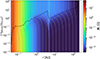 |
Fig. 1. Time evolution of the magnetic field strength over time (normalised in units of the diffusion timescale of the stationary model at the outer DZ boundary, tdiff, stat(rDZ, out)), where the colour-coding represents the magnetic field strength, |B|, at every point in space and time. The gray lines show magnetic flux transport over time, using the effective, vertically averaged magnetic field transport velocity, |

3.2. Remarks on the validity of stationary models
In this work most of our conclusions are drawn from the analysis of stationary PPD models. Since disks are evolving over time, it is important to discuss the validity of using stationary models. In our 1+1D models we use a vertically averaged viscous-α (see Eq. (5), based on the layered viscosity model of Gammie 1996, see also Steiner et al. 2021), which implies that viscous accretion varies in vertical direction between different layers. A localised perturbation changing α(r, z) at some radius r and some height z would lead to an increased or decreased local density, ρ(r, z), and therefore would cause a deviation from a hydrostatic vertical equilibrium at r. Additionally, the vertically averaged α would change at r, which over time would lead to a bump or gap in Σ(r). The development of such gaps or bumps would occur on the local viscous timescale, tvisc, whereas the return to a local vertical hydrostatic equilibrium would happen on the local dynamical timescale, tdyn (e.g. Delage et al. 2022). Therefore, an approximate stationary model can be understood as a time-averaged disk, where such local perturbations are smoothed out under the assumption that the relaxation to a hydrostatic equilibrium happens much faster than the development of a bump or gap in Σ, or tdyn(r)≪tvisc(r).
Additionally, we have to discuss the validity of a stationary large-scale magnetic field, which can be argued similarly in comparing the timescale of global magnetic field evolution to the timescale at which such perturbations typically occur. It has been argued by Dudorov & Khaibrakhmanov (2014) that the magnetic field in vertical direction also changes on tdyn. In contrast, the large-scale magnetic field in radial direction evolves on the local diffusion timescale, tdiff, which requires tdyn ≪ tdiff for a valid temporal averaging of local large-scale magnetic field perturbations.
Finally, PPDs typically disperse after ∼1 − 4 Myrs (e.g. Delage et al. 2022; Ben et al. 2025), which raises the question if such disks live long enough to allow the disk and large-scale magnetic field to evolve towards a stationary state (i.e. steady-state accretion with Ṁ = const.). This means that we also have to verify that the global evolution timescales of both disk and large-scale magnetic field, tvisc and tdiff, respectively, are shorter or of the order of typical disk lifetimes (e.g. Delage et al. 2022). In Fig. 2 we can see that the conditions, tdyn ≪ tvisc and tdyn ≪ tdiff, are both fulfilled everywhere in the disk, which allowed us temporally average over local perturbations of the vertical disk structure and vertical large-scale magnetic field profile. Furthermore, Fig. 2 shows that tdiff and tvisc are indeed shorter or of the order of a typical PPD lifetime, which justifies the assumption that the disk is likely to establish (near) steady-state accretion and therefore stationarity over most of its radial extent before it dissolves (e.g. Delage et al. 2022, for a similar argumentation).
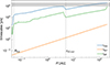 |
Fig. 2. Timescales of our reference model (cf. Table 2) relevant to the long-term evolution of a PPD and a large-scale magnetic field. The solid blue, orange, and green lines correspond to the viscous timescale, tvisc; the dynamical timescale, tdyn; and the magnetic diffusion timescale, tdiff, respectively. The vertical, dashed black lines correspond to the corotation radius, Rcor, and the outer DZ boundary, rDZ, out. Finally, the gray area marks the region between 1 Myr and 4 Myrs and depicts the expected lifetime of a PPD. |
3.3. The reference model
In this section, we describe the details of our reference disk model, especially the large-scale disk magnetic field topology. The field is strongly dependent on the resistivity profile,  , which in turn is dependent on the ionisation fraction, xe(r, z). Therefore, we investigated in more detail the vertical and radial profile of xe and η, which then can be used to construct the conductivity-weighted vertical resistivity average,
  , counteracting advection.
3.3.1. Large-scale magnetic field profile:
We present and analyse the stationary magnetic field structure. As already discussed in Sect. 3.1, the field in the inner disk is dominated by the stellar dipole field (see Eqs. (14)–(16)). Since Bz, ⋆ ∝ r−3, the vertical magnetic field, Bz, in the inner disk also follows this power law (see (a) in Fig. 3). The field evolution in the outer disk is strongly influenced by AD, which according to an analytical model from (Dudorov & Khaibrakhmanov 2014), should lead to a dependency Bz ∝ r−5/8 in the case of an irradiated disk, which we can verify with our model (see (a) in Fig. 3). Amplification of the fossil field in the outer region is roughly Bz/Bz(t = 0)≈10, whereas in the inner disk, due to the dominant stellar field component, almost no amplification is observed. However, the disk field is advected inwards and a radial field component at the disk surface, Brs, develops, which leads to an inclination of the large-scale field with respect to the disk normal (see (b) in Fig. 3). The value of 30° shown in (b) of Fig. 3 corresponds to the critical field inclination, for which cold MCWs can be launched (e.g. Ogilvie 1997; Ogilvie & Livio 2001, and Sect. 4.2).
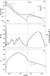 |
Fig. 3. Poloidal stationary magnetic field profile of our reference model (see Table 2). Panel (a) shows both the vertical and radial magnetic field component at the surface, Bz and Brs, respectively. Panel (b) depicts the ratio of Brs/Bz, which is a measure for the inclination of the field lines, whereas panel (c) shows the magnetic plasma beta β0 at the disk midplane. The vertical dashed line correspond to the corotation radius, Rcor, and rDZ, out, respectively. The dotted, gray lines in panels (a) and (c) describe the corresponding values at t = 0, whereas the horizontal dotted line in panel (b) denotes a surface angle of 30° with respect to the midplane normal. |
Inside the DZ close to rDZ, out, the radial field, Brs, decreases significantly compared to its value outside the DZ. This can be explained by comparing the viscous timescale, tvisc, to tdiff, stat: If tdiff, stat is significantly shorter than tvisc, then the large-scale field diffuses outwards before any significant inward-directed advection takes place. As a consequence, field lines are only weakly inclined and Brs stays small compared to Bz (see zone around tdiff, DZ in Fig. 4). Only very close to the inner rim tdiff, stat/tvisc ≈ 1, which means that there Brs ≈ Bz (cf. spike in Brs close to the inner rim in (b) of Fig. 3 and in Fig. 4). This steep increase in tdiff, stat close to rin is a result of three effects, which occur in a very narrow radial region close to the inner rim: (i) At the transition from optically thin to optically thick gas a dip in Tgas (for details see below paragraph about the temperature profile and (b) of Fig. 6 leads to a reduced xe,th and consequently to a larger  , which is equivalent to a shorter tdiff, stat. (ii) However, just slightly further inwards, the stellar irradiation starts to dominate the disk temperature, which leads to rising Tgas (see (b) of Fig. 6) and a steep decrease of
  once more (or equivalently to a sharp increase of tdiff, stat, see Fig. 4) (iii) Closest to rin,
  rises again (equivalently tdiff, stat becomes shorter) slightly towards rin which is due to small Σ and relatively large |B| provided by the stellar dipole field (we recall that ηA ∝ |B|2 ρ−2, also see Eq. (59)).
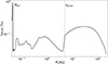 |
Fig. 4. Comparison of the viscous timescale, tvisc, and the diffusion timescale, (tdiff, stat). The vertical dashed lines close to the inner rim and at ∼4 AU represent Rcor and rDZ, out, respectively. |
The magnetic plasma beta at the midplane, β0, describes the relative importance of the large-scale field in the disk. We start the time evolution with a fossil field, which corresponds to β0(r = rout) = 102 at the outer disk rim, rout. In the AD-dominated outer disk, the model of Dudorov & Khaibrakhmanov (2014) predicts a radial dependency β0 ∝ r−3/2 in the case of an irradiated, optically thick disk, which our results also reflect (see (c) in Fig. 3).
3.3.2. Resistivity profile:
The ionisation fraction profile in radial and vertical direction, xe(r, z), is necessary to calculate the corresponding OD and AD profiles, ηO and ηA, respectively. Both thermal and non-thermal ionisation are taken into account (see Sect. 2.5) and show that the innermost region (r ≤ 0.044 AU) is optically thin due to low Σ and the gas temperature, Tgas, is dominated by stellar irradiation. Hence, the very inner disk has a high xe; however, at ∼0.044 AU, the disk becomes sufficiently dense to turn optically thick for stellar radiation and the primary heating process transitions from stellar irradiation to viscous heating. Additionally, the disk has a DZ between 0.06 AU ≲ r ≲ 5 AU, where the inner part of the DZ close to the midplane r ≲ 0.2 AU is subject to thermal ionisation due to viscous heating (cf. region of large ionisation in the inner disk region close to the midplane in (a) of Fig. 5). Above z ≈ Hp, thermal ionisation is not effective anymore, since the disk is hydrostatically stratified and ρ above Hp becomes very small. Finally, the upper disk is penetrated mainly by X-rays and cosmic rays, yielding an expected significant xe,nth in the surface layer.
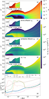 |
Fig. 5. For better understanding of the regimes of thermal and non-thermal ionisation, the radial and vertical profiles of (a) ionisation fraction, xe; (b) the contribution of OD, ηO; (c) the contribution of AD, ηA; and (d) the combined resistivity, η(r, z) = ηO(r, z)+ηA(r, z), are plotted for our reference model, which is explained in Sect. 3.1 (cf. Table 2). The dashed gray lines in (a)–(d) correspond to specific heights above the disk midplane (z = 0, z = Hp, |


Ohmic diffusion, ηO, is only significant inside the DZ, which is also in agreement with predictions made by other authors (e.g. Bai & Stone 2013; Delage et al. 2022). Interestingly, the DZ also spans above (and below) the thermally ionised region in the inner disk, which means that the very weakly ionised gas is shifted to intermediate heights, where thermal ionisation cannot be maintained due to low gas density and non-thermal ionisation sources cannot penetrate deep enough to ionise the gas. The disk surface layer is sufficiently well ionised by non-thermal processes, such that ηO ∝ xe−1 is very inefficient in the disk surface (see (b) of Fig. 5).
Ambipolar diffusion, ηA, is effectively quenched in the thermally ionised disk region, which is due to both high gas density, ρ, and large xe (we recall that ηA ∝ |B|2 ρ−2 xe−1, see Eq. (65)). Inside the DZ, ηA is also negligible compared to ηO due to its strong dependency on ρ. In the surface layer as well as in the outer disk; however, AD becomes the dominant diffusion process. The magnetic field strength, |B|, is roughly independent of height, z, and therefore the relative importance of |B| compared to ρ increases with z (see (c) of Fig. 5). The combined resistivity profile η = ηO + ηA is plotted in panel (d) of Fig. 5. The regions of low η are the thermally ionised disk region, a thin layer at intermediate height z inside the DZ and in the outer disk close to the midplane. Recalling Eq. (26), the vertical averaging process of  favours layers of low η, as in those regions magnetic flux transport,
  , is more efficient. As explained in Sect. 2.5 it is important for our model to vertically average the resistivity profile,
  , due to constraint of a 1+1D model. Therefore, we evaluated (ηO + ηA)(r, z) at five different heights, including at the midplane, the pressure scale height, and the magnetic surface: z = 0, z = Hp, and zB, respectively. Additionally, for
  to also incorporate the effects of the DZ above the thermally ionised region and of the disk layer of comparatively low resistivity between the DZ and the surface layer,
  is evaluated at two additional heights,
  and
and  to adequately describe that in different radial sections different vertical layers contribute dominantly to
  (see (e) of Fig. 5):
-
In the thermally ionised region (r ≲ 0.3 AU), η is dominated by the vertical disk layers close to the disk midplane (the dashed orange line and dash-dotted green line are closest to the blue full line for r ≲ 0.3 AU, see panel (e) of Fig. 5).
-
In the region inside the DZ, but further out than the thermally ionised region (0.3 AU ≲ r ≤ rDZ, out), η is dominated by a region above the vertical extent of the DZ but deep enough below the disk surface for non-thermal radiation not ionising the gas. In this intermediate region, AD is the dominant non-ideal diffusion process (the purple dash-dotted line is very close to the full blue line in this region, see panel (e) of Fig. 5).
-
Outside of the DZ (r ≥ rDZ, out), the disk is dominated by AD, which is least effective close to the disk midplane and therefore most dominant for calculating the average
 (the dashed orange line and dash-dotted green line are very close to the blue full line, see panel (e) of Fig. 5).
For comparison, the turbulent resistivity, ηt, resulting from a magnetic Prandtl number, 𝒫 = 1, is also included in the vertical average of  and is taken to be vertically constant, which means that ηt is added at every height to η(r, z). It has been pointed out by other authors (e.g. Dudorov & Khaibrakhmanov 2014) that ηt is only important in the innermost hot disk with high xe (cf. the magenta line in panel (e) of Fig. 5).
3.3.3. Temperature profile:
The disk temperature profile, Tgas(r), is important for determining the thermal gas pressure, Pgas, as well as the pressure scale height, Hp, and the magnetic surface, zB. All of those quantities are important to get the magnetic flux transport and the large-scale magnetic field topology, (Brs(r), 0, Bz(r))T. The optically thick regions of the disk are dominated by viscous heating, whereas Tgas in the optically thin regions is determined by stellar irradiation and the ambient temperature (for implementation details, see Ragossnig et al. 2020; Steiner et al. 2021).
We highlight one important temperature feature close to the inner edge of the disk, resulting in a distinct dip in the temperature of the disk (see (b) of Fig. 6). At the transition between the optically thick (white) and the optically thin (grey) region, we compare the individual energy contributions. The pressure work rate, Pgas∇⋅u, has a negative sign, which means that pressure aids the gas to be pushed inwards due to −ΔPgas < 0 in this area. Additionally, the net energy advected by the radial gas flow into a disk annulus just outside Rcor is positive, because of the stellar torques acting on the inner disk. However, for r < Rcor the stellar dipole brakes the gas and gas starts to fall radially faster towards the star. This leads to Ėadv < 0, because more material exits than enters any disk annulus at r < Rcor (see (a) of Fig. 6). The combined effect of pressure work and advection at r ≈ Rcor, Pgas ∇ · u + Ėadv < 0, leads to a net drain of inner energy e from the disk annuli in this area and is equivalent to a lower Tgas, 0. For our reference model, this leads to a drop below Tgas, 0 < 1500 K (see (b) of Fig. 6). At this temperature, some dust can still survive (e.g. Ferguson et al. 2005).
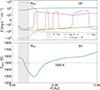 |
Fig. 6. Panel (a), energy contributions to the overall inner energy budget for every disk annulus at radius r. Q : ∇u, Γ − Λ, Pgas ∇⋅u, 4 π Σ κR(J − S), and Ėadv, denote energy rates per unit volume due to viscous heating, heating or cooling over the surface, work done by gas pressure per unit time, radial radiation flux, and net inner energy advection, respectively (see Eq. (3)). Panel (b), plot of the midplane gas temperature, Tgas, 0. The vertical dashed line in all panels denotes the corotation radius, Rcor, and the gray area marks the optically thin region in the inner disk. |
3.4. Variation of stellar parameters
In this section we investigate the influence of stellar magnetic field strength, |B⋆|, rotation period, P⋆, and the X-ray luminosity, LX, on the large-scale magnetic field topology. All stellar parameters are held constant throughout the magnetic field evolution towards the steady-state solution. The parameter range for P⋆ is varied between 4 and 6 days, which is based on observations of young stellar objects in the Orion Nebular Cluster (Herbst et al. 2002). We choose |B⋆| to range from 200 G to 1 kG by referring to the analysis of observed magnetic maps published by Johnstone et al. (2014). We also study the effects of a varying X-ray luminosity, LX, by lowering and increasing our reference value of LX = 1030 erg s−1 by a factor of 10, which is well within the limits of observations made by Preibisch et al. (2005).
3.4.1. Influence of stellar rotation period:
A longer P⋆ yields Rcor and rin moving radially outwards (see Gehrig et al. 2022, and all panels of Fig. 7). Different rotation periods, P⋆, do not have any significant influence on the disk structure or the magnetic field topology outside of r ≳ 0.3 AU (see (b), (d) and (f) of Fig. 7). In the inner disk, however, the disk and large-scale magnetic field have a dependency on P⋆. The stellar magnetic field just outside Rcor accelerates the disk gas, therefore counteracting viscous accretion, which is usually referred as ‘propeller effect’ (e.g. Steiner et al. 2021). This leads to accumulation of mass in the area outside Rcor in the disk region Rcor ≤ r ≲ 0.3 AU. A higher Σ diminishes xe,nth and therefore increases η(r, z) in the disk layers at intermediate heights. However, those intermediate-height disk layers are essentially defining  in the disk for Rcor ≤ r ≲ 0.3 AU (see (e) of Fig. 5); hence
  is increased in this region (see (e) of Fig. 7). Close to Rcor, we observe that
  increases significantly more for slow rotating stars. This is due to lower Tgas, 0 for larger r, leading to a lower xe and therefore to a larger
  . In panel (b), we can then see the expected result that a larger
  causes less inclined field lines. For r < Rcor the narrow and steep increase of Brs/Bz (see Sect. 3.3) becomes less pronounced for larger P⋆ (see (c) of Fig. 7). This is because not only Rcor but also the optically thin region close to rin shifts towards larger radii. There, the disk is colder (compared to faster rotating stars), which results in less effective thermal ionisation and a less pronounced dip of η in the innermost disk region.
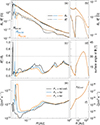 |
Fig. 7. Comparison of the magnetic field topology between our reference model (P⋆ = 4 days, black) and two stars with P⋆ = 5 days (blue) and P⋆ = 6 days (orange). The vertical dashed lines mark the positions of Rcor and are colour-coded accordingly. Panels (a) and (b) show the vertical and radial magnetic field profiles in the inner and outer disk, respectively. Panels (c) and (d) depict the conductivity-weighted, vertically averaged resistivity |

3.4.2. Influence of stellar magnetic field strength:
Different stellar magnetic field strengths, |B⋆|, do not alter the large-scale field topology in the outer disk for r ≳ 1 AU (see (b), (d), and (f) of Fig. 8). The inner radius, rin, moves closer to the star for weaker stellar dipole fields (Steiner et al. 2021, and Fig. 8), and hence the disk close to rin becomes hotter. This means that for weaker |B⋆|, even in the region of the dip in Tgas, 0 (see Sect. 3.3), the gas stays hot enough for efficient thermal ionisation and leads to a less distinct spike in Brs/Bz for weaker dipole fields (see (c) of Fig. 8). The magnetic field is also altered inside the DZ, which is caused by a different mechanism as in the very inner disk. A larger |B⋆| also leads to a larger large-scale field strength, Bd, in the radial range 0.1 AU ≲ r ≲ 1 AU (see (a) of Fig. 8). In this region, AD, ηA, dominantly contributes to  (Sect. 3.3). Since ηA ∝ B2, a small value of B⋆ results in a smaller resistivity and the large-scale field is dragged inwards more efficiently. Consequently, the surface angle increases (see (b) and (c) of Fig. 8). This effect is even amplified by the fact that a weaker field provides less resistance against bending, causing the difference between different stellar magnetic field strengths to be even more significant.
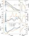 |
Fig. 8. Same as Fig. 7 but for different values of |B⋆|. The stellar field strengths, |B⋆|, of 1 kG, 500 G, and 200 G respectively correspond to the black, blue, and orange lines. |
3.4.3. Influence of stellar X-ray luminosity:
The stellar X-ray luminosity, LX, is directly proportional to the non-thermal X-ray ionisation, both direct ionisation Eq. (73) and through scattering Eq. (74). Therefore, it is expected that an increase of LX causes a higher non-thermal ionisation fraction, xe, nth, in the upper disk layers, thus leading to a reduced vertically averaged resistivity,  . This is indeed the case for our models (see Fig. 9); however in the inner disk region r ≲ 0.15 AU the dominant ionisation mechanism is thermal ionisation, which explains the lack of variation in this disk region (see Fig. 9).
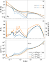 |
Fig. 9. Same as in Fig. 7 but for different stellar X-ray luminosities, LX, reaching from 1029 erg s−1 to 1031 erg s−1. |
A lower  means a more effective coupling of the large-scale field to the disk, which leads to more magnetic flux transport towards the star and therefore a stronger large-scale disk field (see (a) in Fig. 9), which in turn increases ηA and so lessens the effect of a stronger LX to a certain degree, but remains of minor significance compared to the effect of increased xe,nth. More effective magnetic field dragging also results in a stronger radial large-scale field component, Brs, as well as a larger ratio Brs/Bz, which corresponds to a larger surface angle of the resulting field (see (b) and (c) of Fig. 9). Contrary to the variation of P⋆ and B⋆, also the magnetic field in the outer parts of the disk is influenced by a varying LX. This is also expected, as the dominant ionisation process in the outer disk is non-thermal ionisation. In summary, the effects of LX on the large-scale field topology lead to a stronger large-scale field for larger values of LX and additionally allow for a significantly stronger inclined large-scale field for all radii r ≳ 0.2 AU.
3.5. Influence of the mass transport rate
We investigate how the variation of Ṁ influences the magnetic field in the disk. In the picture of a steady-state disk and the viscous α description, the mass transport rate through the disk defines the surface density profile. A higher Ṁ results in a larger DZ, which extends further outwards due to a larger Σ and therefore to lower non-thermal ionisation in the layers below the disk surface (e.g. Steiner et al. 2021; Delage et al. 2022). The outer boundary of the disk, rout, is defined by the condition of Σ = 1 g cm−2 (Vorobyov et al. 2020) and hence also shifts towards larger radii for a more massive disk.
Having a more massive and larger disk, we expect the large-scale magnetic field to react in the outer disk in the following way: A larger disk can drag (and amplify) the fossil field inwards from further out. Hence, for a given r in the outer disk (sufficiently far away from the outer disk boundary to rule out any boundary effects), the large-scale field is expected to be slightly stronger. (ii) A lower xe due to a larger Σ, and therefore a reduced xe,nth, results in less magnetic flux transport and leads to a less inclined field. We can confirm both of those expectations with our results (see r ∼ 10 AU in (b) and (d) of Fig. 10) The increased field inclination in the DZ for a more massive disk can be explained in the following way: A more massive disk is more extended in the vertical direction (larger Hp), which means that the vertical disk layers contributing most to magnetic flux transport are at larger z. As stated in Sect. 2, in our model ur ∝ z2 (cf. Eq. (40)) and for the vertical average  the disk layers of low resistivity are given more weight (cf. Eq. (27)). This means that for a more massive disk, magnetic flux transport is faster in the layers above the dead zone, which results in a larger inclined large-scale field (cf. (d) of Fig. 10).
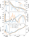 |
Fig. 10. Same as in Fig. 7 but for different Ṁ. The colour-coded vertical dashed lines correspond to the outer dead zone boundaries, rDZ, out, of the respective disk model. |
In the inner disk, rin also shifts towards smaller radii for a larger Ṁ due to increased ram pressure (for details cf. Steiner et al. 2021, cf. also (a), (c) and (e) of Fig. 10). Our model with Ṁ = 10−9 M⊙ yr−1 shows a large increase in  (compared to the other models with higher Ṁ) at the transition from an optically thick to an optically thin disk (cf. Sect. 3.3 and panel (b) of Fig. 6), because the disk is colder, both due to less viscous heating and its larger radial distance from the star. The strong diffusion of Brs in this region is superimposed with the radial contribution of Br, ⋆s (cf. Eq. (15) results in Brs changing sign in a very narrow region. The spike in Brs/Bz is not visible for a disk with low Ṁ, because the disk is truncated before Tgas, 0 rises high enough to decrease
  sufficiently (cf. (e) of Fig. 10. In contrast, for larger disk masses the dip in Tgas, 0 is less distinct due to its proximity to the star, which also results in a less pronounced spike in inclination compared to our reference model (cf. (c) of Fig. 10).
4. Discussion
In this paper we have presented long-term, hydrodynamic simulations of a PPD with a large-scale magnetic field until the disk and large-scale magnetic field become stationary. This allowed us to iterate further on the work done by other authors (e.g. Lubow et al. 1994; Guilet & Ogilvie 2014), who have evolved a large-scale field threading a simplified, stationary disk, but whose models lack the inclusion of laminar, non-ideal effects, which in our case are limited to OD and AD. Additionally, due to the implicit time integration scheme of TAPIR, we are able to include the very inner disk region and therefore include the impact of a stellar dipole both on the inner disk and on the large-scale field by using the hydrodynamic disk evolution model of e.g. Steiner et al. (2021), Gehrig et al. (2022).
Our results show that the large-scale field develops on the magnetic diffusion timescale, which differs between the DZ and the region further outwards, causing a distinction between the field inside and outside the DZ. Furthermore, the large-scale field is significantly bent in the very inner disk and in the outer disk (outside the DZ), but not in the dead zone close to the outer dead zone rim, which is in agreement with simulations carried out by other authors (e.g. Bai & Stone 2013; Zhu & Stone 2018). Additionally, we show that varying stellar parameters such as stellar magnetic field strength, |B⋆|; X-ray luminosity, LX; and stellar rotation period P⋆ can influence the large-scale magnetic field topology by altering the large-scale field strength and inclination. Our study also reveals which parameters influence the large-scale field in the very inner disk, the DZ, or the outer regions of the disk.
4.1. Comparison with recent studies
Our approach is novel in that it is able to evolve a PPD, including the very inner disk, threaded by a large-scale field magneto-hydrodynamically up to the point where the model becomes stationary without imposing any external stationarity constraint on it. Comparing our model to recent studies using other methods to determine the large-scale field structure in a PPD is therefore important to provide additional justification for our approach.
Dudorov & Khaibrakhmanov (2014) use a standard, geometrically thin, α-viscosity accretion disk of Shakura & Sunyaev (1973) to describe the disk and also include stellar irradiation as an additional heating source apart from viscous heating. A significant difference compared to our model is that they neglect radial magnetic flux transport, which makes the calculation of the external magnetic field solution at each time step unnecessary (e.g. Ogilvie 1997; Guilet & Ogilvie 2014) and a constant fossil field description suffices. By contrast, our model incorporates a changing external field due to radial dragging, which also influences the vertical profile of Br inside the disk (e.g. Guilet & Ogilvie 2012; Leung & Ogilvie 2019) and therefore leads to changes in the magnetic field profiles compared to Dudorov & Khaibrakhmanov (2014). The radial profiles of Bz and Brs compare qualitatively well with our results. Moreover, the dependency of dust grain size and LX agrees well with our findings; however, in the very inner disk there are differences: (i) The disk of Dudorov & Khaibrakhmanov (2014) is everywhere optically thick, which is not the case close to the inner boundary for a more realistic inner disk boundary, which leads to a different temperature profile close to the inner rim and hence influences xe as well as η. (ii) No stellar dipole has been modelled in their work, which would alter the disk structure around the corotation radius (Steiner et al. 2021) and also influences the large-scale disk field close to the inner rim. Notably, we obtain less inclined field lines than Dudorov & Khaibrakhmanov (2014) in the inner disk, which is a combined effect of an optically thin inner disk and a more realistic inner boundary. Additionally, we don’t include a toroidal field component, Bφs, in the disk exterior above and below the disk, as this would add the complexity of launching magnetically induced outflows. Dudorov & Khaibrakhmanov (2014) include Bφs, but do not consider outflows in their model.
We also compared our results to both Mohanty et al. (2018) and Delage et al. (2022), as the authors of both papers use an alternative approach to determine the large-scale magnetic field structure. The primary focus of those studies is to determine the effect of the magnetic field strength and non-ideal MHD effects on the α-viscosity and therefore on the disk structure. Nevertheless, the determination of the ionisation fraction, xe, is implemented analogously: Mohanty et al. (2018) use thermal ionisation in the inner disk, whereas non-thermal ionisation in our models is analogous to Delage et al. (2022). In both papers, a standard diffusion disk model is used to describe a stationary disk, which especially in the inner disk leads to differences between the disk structure in Mohanty et al. (2018) and our model. A diffusion approach cannot take into account any pressure gradients occurring in the inner disk and is not able to account for the effect of a stellar dipole (cf. Steiner et al. 2021). Therefore, the Σ-profile in our disk differs from the model in Mohanty et al. (2018). Moreover, they used a constant opacity κR = 10 cm2 g−1, which is different from κR in our models, as we obtained a small dusty ring just outside the optically thin region closest to the inner disk rim for most of our models. This opacity feature, together with the ionised, strongly heated innermost disk, leads in our simulations to a large inclination of the large-scale disk field very close to the star. However, Mohanty et al. (2018) uses an α-viscosity, which is dependent on the magnetic field strength. This results in α ≈ 0.1 in the very inner disk and is a factor 10 higher than our adopted value of αMRI = 0.01 (cf. Table 2). Therefore, the disk structure in the inner disk is accreting more effectively, which yields a less steep increase in Σ for larger r and a DZ inner boundary further outwards. The most notable difference in both Mohanty et al. (2018) and Delage et al. (2022) with respect to the determination of the large-scale field strength in the disk is their use of an iterative approach: To obtain a stationary disk the condition Ṁ = const. has to be fulfilled. The α-viscosity at every radius determines Ṁ and is dependent on the large-scale field strength (root-mean-square (rms) field, cf. Sano et al. 2004) under the assumption of a maximally efficient MRI. Then, iteratively, a disk structure can be obtained with Ṁ = const. and a corresponding α and magnetic field. This approach cannot account for an external fossil field or a stellar dipole field threading the inner disk, since the field is solely determined by the condition of maximally efficient MRI. There is no evidence that MRI determines the large-scale field strength and not vice versa (also mentioned and discussed by Delage et al. 2022). The results for the radial profile of |B| in Delage et al. (2022) differ from our results especially in the DZ, where their magnetic field strength follows a power-law over the whole disk, contrary to our results, where a DZ has a clear impact on the radial profiles of Bz and Brs.
4.2. Implications of large-scale field inclination
The inclination angle of the large-scale field lines is a crucial parameter in determining the existence and strength of magnetocentrifugally accelerated outflows (e.g. Ogilvie & Livio 1998, 2001; Campbell 1999). We adopt the simple wind model of Ogilvie & Livio (1998) for a rough estimate of the wind mass loss, Ṁwind, which we could expect for a MCW launching from the disk surface. In accordance with our two-zone model of Guilet & Ogilvie (2012), the large-scale field is assumed to be force-free above the disk, which results in rigidly rotating field lines up to the Alfvénic surface (the surface above the disk where the wind velocity surpasses the Alfvén-velocity),
 (83)
(83)
where i denotes the inclination angle at the disk surface with respect to the midplane normal. We note that we only assume the Alfvénic surface to be located somewhere above the sonic surface and make no effort to determine its actual position in this work. In theory, the Alfvén point along a field line determines how much angular momentum can be transported by the wind, whereas the sonic point determines the mass of the wind flow. Hence, for an estimate of the wind mass, we use that it has to pass through the sonic point at height zsonic and assume that zB < zsonic ≪ r. The last assumption is needed for the approximation of a rigid field line. Then the MCW mass loss, Ṁwind, is determined through (for a much more comprehensive explanation, cf. Ogilvie & Livio 1998, 2001)
 (84)
(84)
 (85)
(85)
 (86)
(86)
Here, ΔΦ denotes the effective centrifugal potential and Ω1s the deviation from Keplerian rotation, ΩK, at the disk surface. We further assume that the MCW is launched at z = zB. The resulting Ṁwind for our reference model is shown in Fig. 11 and reveals that the most favourable regions for a MCW are very close to the inner disk boundary, rin, and in the outer, AD-dominated disk for r > rDZ, out. These regions of increased Ṁwind have also been obtained through simulations performed by other authors (e.g. Armitage 2011; Suzuki et al. 2016; Lesur 2021) and observations (Güdel et al. 2018). Nevertheless, we stress the point that this analysis of MCW mass loss is preliminary and serves the purpose of showing that purely magnetocentrifugally driven winds are possible in disks for realistic α-values and fossil field strengths. We interpret these results as a promising starting point for upcoming simulations, including the effects of MHD outflows. A realistic disk model with MHD outflows has to include the effects of angular momentum loss from the wind, which would lead to increased mass transport and magnetic flux transport, and most likely would lead to the opening of a gap (see Armitage 2011). Additionally, some models suggest an inverted Σ-profile in the case of effective winds (e.g. Suzuki et al. 2016), which further confirms that winds need to be included in our MHD disk evolution model as a next step.
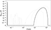 |
Fig. 11. Magnetocentrifugal winds mass loss, Ṁwind, according to Eq. (86) for our reference model (black). All other models discussed in this paper are shown as light grey lines to further illustrate the two dominant wind regimes in the innermost disk and in the outer disk. |
4.3. Variation of the fossil field
The fossil field strength, B∞, in PPDs is a topic of active studies (e.g. Crutcher et al. 2004; Masson et al. 2016; Tsukamoto et al. 2023) and lies in the range of [10−5 G, 10−1 G]. Especially the upper end of this range is intriguing with respect to disk evolution, since such strong magnetic fields can potentially influence disk evolution. Also, with respect to magnetic field evolution in disks, stronger fields are expected to behave differently. A stronger field causes a larger effective resistivity, especially in the outer disk, since there AD is dominant (recall that ηA ∝ |B|2, cf. Eq. (65)).
An increased  then causes less effective magnetic flux transport and a less inclined field geometry in the outer disk (cf. (b) of Fig. 12). Interestingly, the field strength for the two models with β0(rout) = 10 and β0(rout) = 100 is almost indistinguishable for all r ≲ rDZ, out. The model with β0(rout) = 1 yields a larger Bz until the stellar dipole dominates the large-scale field strength. Summarising the results shows that a stronger fossil field, B∞, leads to a less inclined outer disk field, but has no effect on the inner magnetic field topology due to the dominance of the stellar dipole field.
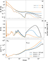 |
Fig. 12. Stationary magnetic field topology for different initial fossil field strengths. The reference model uses a fossil field with β0 = 102 (black) and is compared to two models with a stronger initial field (β0 = 10 (blue) and β0 = 1 (orange)). The panels are the same as in Fig. 8. The vertical dashed lines correspond to Rcor and rDZ, out. |
We emphasise that these results should be taken with a grain of salt, since a basic assumption of our large-scale field model is the two-zone model of Guilet & Ogilvie (2012), Leung & Ogilvie (2019), which assumes a passive magnetic field in the disk (β0 ≫ 1), which is clearly not the case in our model with β0(rout) = 1 (see Sect. 2.4). A large-scale field with β0 ≤ 1 would influence the vertical disk structure (e.g. Ogilvie 1997) and therefore should be taken as a rough estimate of the outer magnetic field structure.
4.4. Model limitations
In this work we conducted long-term MHD simulations of the whole disk while including the very inner disk region r < 0.1 AU, a stellar dipole field, and a large-scale disk field. Covering sufficient time to allow the disk and large-scale field to become stationary, while simultaneously including the inner disk, made it necessary to make various simplifications and assumptions:
-
We used a 1+1D model to conduct our simulations. Hence, the disk and the large-scale field were assumed to be axisymmetric. This constrained us to treat some intrinsically 3D natured phenomena in a simplified way. One example is the inner boundary: The disk is magnetically disrupted by the stellar magnetic field at a certain radius close to the star and is accreted along magnetic funnels (e.g. Romanova et al. 2004). However, such funnels are highly non-axisymmetric, and we therefore used the results of Bessolaz et al. (2008) to construct a physically motivated inner boundary (see Steiner et al. 2021). The disk in the vertical direction is assumed to be hydrostatic, and the disk gas temperature is assumed constant for the hydrodynamic evolution of the disk; however, for the approximation of the ionisation fraction, a temperature profile is used to obtain a better model of the vertical ionisation profile. This is slightly inconsistent, but is not believed to change our results, as the temperature for the hydrodynamic evolution would be included as a density-weighted vertical average and hence would be very close to the midplane value of Tgas (cf. Sect. 2.5).
-
In this work, we focused on studying the poloidal magnetic field structure and did not include toroidal fields. Although we considered the effects of toroidal fields inside the disk, the toroidal field in the disk exterior was assumed to vanish. However, the large-scale field very likely winds up corresponding to a disk field Bφs component in the disk exterior above the disk surface. This, in turn, would imply some outflow coupling to the large-scale field. The launching mechanism could be purely magnetocentrifugal, purely thermal (photo-evaporation), or a combination of both mechanisms (e.g. Lesur 2021). The addition of magnetically and thermally induced outflows and their effects on the long-term disk evolution are the focus of subsequent studies using this model, as it is not constrained to steady-state solutions. This work focused on the effects of a stellar dipole and stellar rotation on the large-scale field topology, while the disk was self-consistently simulated.
-
We did not include FUV radiation in our model, which is expected to strongly ionise the upper atmosphere (e.g. Rab et al. 2017) and can be important in the study of magnetic field evolution, as the large-scale field is radially transported in the disk surface layer in large parts of the disk. Additionally, an ionised upper atmosphere is important for the study of magnetically induced outflows and should be included in upcoming papers aiming to investigate disk evolution, including MCWs.
-
We did not include the effects of EUV heating of the thin, upper disk atmosphere due to secondary processes following the ionisation of the gas. As proposed by Glassgold et al. (2004, 2012), Güdel (2015), up to 50% of the energy deposited in the upper atmosphere is used to heat the gas. For future work, including photoevaporative winds and magnetically driven outflows, these effects should be taken into consideration.
-
The Hall effect is not included in our studies; however, it is the dominant non-ideal, laminar diffusion process in a large radial range of PPDs (e.g. Wardle 2007; Bai & Stone 2017; Leung & Ogilvie 2019). The HE is linked to magnetically induced outflows (e.g. Leung & Ogilvie 2019), which strongly indicates that this effect should be integrated in an upcoming model including magnetised winds. Nevertheless, the treatment of the HE keeps being challenging due to its anisotropic character, which only allows for an approximate treatment in a 1+1D disk model.
-
Dust is treated in our model very simply. The dust-to-gas ratio is assumed to be constant radially and in time, which is very unlikely to ever occur in a realistic disk. Recent work shows that dust can accumulate in rings, which influences the vertical temperature equilibrium and can trigger FU Ori-like outbursts, if those rings occur in the inner disk (e.g. Testi et al. 2014; Vorobyov et al. 2020, 2022). Additionally, we did not include any dust evolution model, ignoring coagulation, fragmentation, or settling of dust grains, which can lead to different ionisation fractions for different dust grain sizes (e.g. Dudorov & Khaibrakhmanov 2014; Delage et al. 2022).
5. Summary and conclusion
In this study, we have extended the 1+1D disk evolution model of Ragossnig et al. (2020), Steiner et al. (2021) with a large-scale magnetic field evolution model (cf. Sect. 2.2). An implicit time integration scheme allowed us to self-consistently include the very inner disk while performing long-term (of the order of the disk viscous timescale) simulations. Including a large-scale field makes it necessary to carefully model the ionisation in the disk both in radial and vertical direction in order to be able to determine the magnetic resistivity in the disk (cf. Sect. 2.5). In our model, we included non-ideal MHD effects, for example, OD and AD. The scientific objectives of this work were twofold. First was to determine the large-scale field topology in a steady-state disk truncated by a stellar dipole. The transition towards a stationary field yielded the following conclusions:
-
Using the conductivity-weighted averaging for the radial magnetic transport velocity,
 , and resistivity,
  , proposed by Guilet & Ogilvie (2012), we were able to include the effects of the vertical disk profile and did not have to ignore magnetic advection at the disk surface (or layers at intermediate heights) in the framework of a 1+1D simulation.
 -
Similar to the results of Guilet & Ogilvie (2014), Dudorov & Khaibrakhmanov (2014), the field is advected inwards effectively in the outer disk and in the inner MRI-active disk. The inclination of the large-scale field lines in the outer DZ is reduced, whereas in the inner DZ, magnetic flux transport in the layers above the DZ leads to a non-negligible inclination.
-
The vertical large-scale field component, Bz, in the inner disk is dominated by the stellar dipole field, whereas the radial field, Brs, depends on the detailed ionisation structure in the disk.
-
The large-scale field inclination in the outer disk is dominated by AD. We managed to reproduce the same power-law dependences for Bz and β0 as, for example, Dudorov & Khaibrakhmanov (2014), which indicates the validity of our approach.
-
The self-consistent hydrodynamical treatment of a magnetically truncated, irradiated disk shows that the radial profiles of Σ, u, and Tgas also lead to a complex large-scale field structure in the inner disk. This is a unique property of our model, as we are not limited by small time steps in the inner disk, and hence long-term simulations of the large-scale field (even though they are conducted with the goal of constructing a stationary model) have not been covered yet (e.g. Dudorov & Khaibrakhmanov 2014; Mohanty et al. 2018; Delage et al. 2022).
The second scientific objective was to perform a parameter study to investigate how stellar and disk parameters influence the large-scale field topology, namely, P⋆, B⋆, LX, and ̇M, and the strength of the fossil field. We found that different stellar parameters influence the large-scale magnetic field topology in different disk regions:
-
The stellar dipole strength, |B⋆|, influences the large-scale field in the inner disk (r < 1 AU) in two ways. First, a weaker dipole field results in disk truncation closer to the star (e.g. Hartmann et al. 2016), where the disk is hotter and therefore has a larger ionisation level. Second, a stronger |B⋆| also increases AD in the region dominated by the dipole and therefore results in a large-scale field with less inclined field lines.
-
A fast or slow rotating star with the rotation period, P⋆, also affects the large-scale field by Rcor being closer to or further away from the star. It only affects the inner disk, r < 0.3 AU, in that a slower rotating star (larger P⋆) leads to a less distinct increase of the field inclination very close to the star.
-
The large-scale field in the DZ and the outer disk is strongly dependent on the X-ray luminosity. A larger LX results in a larger ionisation fraction at the disk surface above the DZ and in the outer disk surface layers. In those disk layers, the large-scale field is advected radially inwards most effectively in those disk regions.
-
Changing Ṁ changes the disk structure and therefore also alters the large-scale field topology. In summary, a larger Ṁ results in a larger inclined field in the dead zone and in rin shifting towards smaller radii, which in turn leads to a pronounced spike in field inclination very close to the star.
This study shows that a large-scale field threading a disk is also dependent on stellar parameters and has non-negligible inclined field lines. Therefore, the next step in this planned series of papers will be to include a wind model dependent on the large-scale field topology and the disk structure. Our simulation framework, TAPIR (e.g. Ragossnig et al. 2020), has an implicit time integration scheme. Therefore, we can conduct long-term simulations covering the whole disk lifetime while including the inner disk, the interaction with a stellar dipole, a large-scale field, and a wind model. This will help answer the question of how disks evolve under the influence of magnetically induced winds in combination with viscous accretion. It will also further allow us to provide estimates on the mass loss and angular momentum loss rates that such winds would produce. An exciting scientific question is whether MCWs lead to an unstable configuration in the disk, as a strongly inclined field triggers a strong MCW, which then removes angular momentum and further increases the inclination. In such a scenario, multiple gaps could be opened in the disk. Equally interesting is the interaction of photoevaporative flows with a large-scale field and the reaction of the large-scale field to high accretion rates during an accretion outburst.
We discuss the timestep-control in our models in Sect. A.
The superscript “s” means that we take the value of the corresponding physical quantity at the disk surface.
The index r(φ) stands for the radial and toroidal velocity component to abbreviate the otherwise identical formulae.
We emphasise that the gray lines in Fig. 1 shall not be confused with field lines, but serve as an indicator, where magnetic flux transport is occurring during field evolution.
Acknowledgments
We thank the referee for the constructive feedback that helped to improve and clarify the manuscript.
References
- Armitage, P. J. 2011, ARA&A, 49, 195 [Google Scholar]
- Armitage, P. J., Livio, M., & Pringle, J. E. 2001, MNRAS, 324, 705 [NASA ADS] [CrossRef] [Google Scholar]
- Asplund, M., Amarsi, A. M., & Grevesse, N. 2021, A&A, 653, A141 [NASA ADS] [CrossRef] [EDP Sciences] [Google Scholar]
- Bai, X.-N., & Goodman, J. 2009, ApJ, 701, 737 [NASA ADS] [CrossRef] [Google Scholar]
- Bai, X.-N., & Stone, J. M. 2011, AAS/Div. Extreme Sol. Syst. Abstr., 2, 36.03 [Google Scholar]
- Bai, X.-N., & Stone, J. M. 2013, ApJ, 769, 76 [Google Scholar]
- Bai, X.-N., & Stone, J. M. 2017, ApJ, 836, 46 [Google Scholar]
- Balbus, S. A., & Hawley, J. F. 1991, ApJ, 376, 214 [Google Scholar]
- Baraffe, I., Homeier, D., Allard, F., & Chabrier, G. 2015, A&A, 577, A42 [NASA ADS] [CrossRef] [EDP Sciences] [Google Scholar]
- Bell, K. R., & Lin, D. N. C. 1994, ApJ, 427, 987 [NASA ADS] [CrossRef] [Google Scholar]
- Ben, G. M., Jose, J., & Hernández, J. 2025, MNRAS, 541, 2246 [Google Scholar]
- Bertrang, G. H. M., Flock, M., & Wolf, S. 2017, MNRAS, 464, L61 [NASA ADS] [CrossRef] [Google Scholar]
- Bessolaz, N., Zanni, C., Ferreira, J., Keppens, R., & Bouvier, J. 2008, A&A, 478, 155 [NASA ADS] [CrossRef] [EDP Sciences] [Google Scholar]
- Blandford, R. D., & Payne, D. G. 1982, MNRAS, 199, 883 [CrossRef] [Google Scholar]
- Brandenburg, A., Nordlund, A., Stein, R. F., & Torkelsson, U. 1995, ApJ, 446, 741 [NASA ADS] [CrossRef] [Google Scholar]
- Brauer, R., Wolf, S., & Flock, M. 2017, A&A, 607, A104 [NASA ADS] [CrossRef] [EDP Sciences] [Google Scholar]
- Campbell, C. G. 1999, MNRAS, 310, 1175 [Google Scholar]
- Cecil, M., Gehrig, L., & Steiner, D. 2024, A&A, 687, A136 [NASA ADS] [CrossRef] [EDP Sciences] [Google Scholar]
- Courant, R., Friedrichs, K., & Lewy, H. 1928, Math. Ann., 100, 32 [Google Scholar]
- Crutcher, R. M., & Kemball, A. J. 2019, Front. Astron. Space Sci., 6, 66 [CrossRef] [Google Scholar]
- Crutcher, R. M., Nutter, D. J., Ward-Thompson, D., & Kirk, J. M. 2004, ApJ, 600, 279 [Google Scholar]
- Delage, T. N., Okuzumi, S., Flock, M., Pinilla, P., & Dzyurkevich, N. 2022, A&A, 658, A97 [NASA ADS] [CrossRef] [EDP Sciences] [Google Scholar]
- Dong, R., Vorobyov, E., Pavlyuchenkov, Y., Chiang, E., & Liu, H. B. 2016, ApJ, 823, 141 [NASA ADS] [CrossRef] [Google Scholar]
- Dorfi, E., & Drury, L. 1987, J. Comput. Phys., 69, 175 [NASA ADS] [CrossRef] [Google Scholar]
- Dudorov, A. E., & Khaibrakhmanov, S. A. 2014, Ap&SS, 352, 103 [NASA ADS] [CrossRef] [Google Scholar]
- Ferguson, J. W., Alexander, D. R., Allard, F., et al. 2005, ApJ, 623, 585 [Google Scholar]
- Ferreira, J., Dougados, C., & Cabrit, S. 2006, A&A, 453, 785 [NASA ADS] [CrossRef] [EDP Sciences] [Google Scholar]
- Gammie, C. F. 1996, ApJ, 457, 355 [Google Scholar]
- Gehrig, L., & Vorobyov, E. I. 2023, A&A, 673, A54 [NASA ADS] [CrossRef] [EDP Sciences] [Google Scholar]
- Gehrig, L., Steiner, D., Vorobyov, E. I., & Güdel, M. 2022, A&A, 667, A46 [NASA ADS] [CrossRef] [EDP Sciences] [Google Scholar]
- Glassgold, A. E., Najita, J., & Igea, J. 2004, ApJ, 615, 972 [NASA ADS] [CrossRef] [Google Scholar]
- Glassgold, A. E., Galli, D., & Padovani, M. 2012, ApJ, 756, 157 [Google Scholar]
- Güdel, M. 2015, EPJ Web Conf., 102, 00015 [Google Scholar]
- Güdel, M., Eibensteiner, C., Dionatos, O., et al. 2018, A&A, 620, L1 [NASA ADS] [CrossRef] [EDP Sciences] [Google Scholar]
- Guilet, J., & Ogilvie, G. I. 2012, MNRAS, 424, 2097 [Google Scholar]
- Guilet, J., & Ogilvie, G. I. 2014, MNRAS, 441, 852 [NASA ADS] [CrossRef] [Google Scholar]
- Hartmann, L., Herczeg, G., & Calvet, N. 2016, ARA&A, 54, 135 [Google Scholar]
- Herbst, W., Bailer-Jones, C. A. L., Mundt, R., Meisenheimer, K., & Wackermann, R. 2002, A&A, 396, 513 [EDP Sciences] [Google Scholar]
- Hubeny, I. 1990, ApJ, 351, 632 [NASA ADS] [CrossRef] [Google Scholar]
- Hueso, R., & Guillot, T. 2005, A&A, 442, 703 [NASA ADS] [CrossRef] [EDP Sciences] [Google Scholar]
- Irwin, J., & Bouvier, J. 2009, in The Ages of Stars, eds. E. E. Mamajek, D. R. Soderblom, & R. F. G. Wyse, IAU Symp., 258, 363 [Google Scholar]
- Jackson, J. D. 1999, Classical Electrodynamics, 3rd edn. (New York, NY: Wiley) [Google Scholar]
- Jankovic, M. R., Owen, J. E., Mohanty, S., & Tan, J. C. 2021, MNRAS, 504, 280 [NASA ADS] [CrossRef] [Google Scholar]
- Johns-Krull, C. M., Valenti, J. A., & Koresko, C. 1999, ApJ, 516, 900 [Google Scholar]
- Johnstone, C. P., Jardine, M., Gregory, S. G., Donati, J. F., & Hussain, G. 2014, MNRAS, 437, 3202 [Google Scholar]
- Khaibrakhmanov, S. A., & Dudorov, A. E. 2022, Astron. Rep., 66, 872 [Google Scholar]
- Lankhaar, B., & Teague, R. 2023, A&A, 678, A17 [NASA ADS] [CrossRef] [EDP Sciences] [Google Scholar]
- Lee, C.-F. 2020, A&ARv, 28, 1 [NASA ADS] [CrossRef] [Google Scholar]
- Lesur, G. R. J. 2021, A&A, 650, A35 [NASA ADS] [CrossRef] [EDP Sciences] [Google Scholar]
- Lesur, G., Kunz, M. W., & Fromang, S. 2014, AAP, 566, A56 [Google Scholar]
- Lesur, G., Flock, M., Ercolano, B., et al. 2023, in Protostars and Planets VII, eds. S. Inutsuka, Y. Aikawa, T. Muto, K. Tomida, & M. Tamura, ASP Conf. Ser., 534, 465 [NASA ADS] [Google Scholar]
- Leung, P. K. C., & Ogilvie, G. I. 2019, MNRAS, 487, 5155 [Google Scholar]
- LeVeque, R. J., Mihalas, D., Dorfi, E. A., & Müller, E. 1997, Astrophysics of Planet Formation (Saas-Fee Advanced Course 27. Lecture Notes 1997 Swiss Society for Astrophysics and Astronomy) [Google Scholar]
- Lubow, S. H., Papaloizou, J. C. B., & Pringle, J. E. 1994, MNRAS, 268, 1010 [NASA ADS] [CrossRef] [Google Scholar]
- Masson, J., Chabrier, G., Hennebelle, P., Vaytet, N., & Commerçon, B. 2016, A&A, 587, A32 [NASA ADS] [CrossRef] [EDP Sciences] [Google Scholar]
- Mohanty, S., Jankovic, M. R., Tan, J. C., & Owen, J. E. 2018, ApJ, 861, 144 [Google Scholar]
- Nakamoto, T., & Nakagawa, Y. 1994, ApJ, 421, 640 [Google Scholar]
- Ogilvie, G. I. 1997, MNRAS, 288, 63 [NASA ADS] [Google Scholar]
- Ogilvie, G. I., & Livio, M. 1998, ApJ, 499, 329 [NASA ADS] [CrossRef] [Google Scholar]
- Ogilvie, G. I., & Livio, M. 2001, ApJ, 553, 158 [Google Scholar]
- Ohashi, S., Kataoka, A., Nagai, H., et al. 2018, ApJ, 864, 81 [NASA ADS] [CrossRef] [Google Scholar]
- Pollack, J. B., McKay, C. P., & Christofferson, B. M. 1985, Icarus, 64, 471 [NASA ADS] [CrossRef] [Google Scholar]
- Preibisch, T., Kim, Y.-C., Favata, F., et al. 2005, ApJS, 160, 401 [NASA ADS] [CrossRef] [Google Scholar]
- Rab, C., Güdel, M., Padovani, M., et al. 2017, A&A, 603, A96 [NASA ADS] [CrossRef] [EDP Sciences] [Google Scholar]
- Ragossnig, F., Dorfi, E. A., Ratschiner, B., et al. 2019, 1+1D Implicit Disk Computations, 3rd edn. (Computer Physics and Communications) [Google Scholar]
- Ragossnig, F., Dorfi, E. A., Ratschiner, B., et al. 2020, Comp. Phys. Commun., 256, 107437 [Google Scholar]
- Reyes-Ruiz, M., Pérez-Tijerina, E., & Sánchez-Salcedo, F. J. 2004, Rev. Mex. Astron. Astrofis. Conf. Ser., 22, 113 [Google Scholar]
- Romanova, M. M., Ustyugova, G. V., Koldoba, A. V., & Lovelace, R. V. E. 2002, ApJ, 578, 420 [Google Scholar]
- Romanova, M. M., Ustyugova, G. V., Koldoba, A. V., & Lovelace, R. V. E. 2004, ApJ, 610, 920 [Google Scholar]
- Sano, T., Inutsuka, S.-I., Turner, N. J., & Stone, J. M. 2004, ApJ, 605, 321 [NASA ADS] [CrossRef] [Google Scholar]
- Shakura, N. I., & Sunyaev, R. A. 1973, A&A, 24, 337 [NASA ADS] [Google Scholar]
- Simon, J. B., Bai, X.-N., Armitage, P. J., Stone, J. M., & Beckwith, K. 2013, ApJ, 775, 73 [NASA ADS] [CrossRef] [Google Scholar]
- Spitzer, L. 1978, Physical Processes in the Interstellar Medium (Wiley-Interscience) [Google Scholar]
- Steiner, D., Gehrig, L., Ratschiner, B., et al. 2021, A&A, 655, A110 [NASA ADS] [CrossRef] [EDP Sciences] [Google Scholar]
- Suzuki, T. K., Ogihara, M., Morbidelli, A., Crida, A., & Guillot, T. 2016, A&A, 596, A74 [NASA ADS] [CrossRef] [EDP Sciences] [Google Scholar]
- Tang, Y.-W., Dutrey, A., Koch, P. M., et al. 2023, ApJ, 947, L5 [NASA ADS] [CrossRef] [Google Scholar]
- Testi, L., Birnstiel, T., Ricci, L., et al. 2014, in Protostars and Planets VI, eds. H. Beuther, R. S. Klessen, C. P. Dullemond, & T. Henning, 339 [Google Scholar]
- Tsukamoto, Y., Maury, A., Commercon, B., et al. 2023, in Protostars and Planets VII, eds. S. Inutsuka, Y. Aikawa, T. Muto, K. Tomida, & M. Tamura, ASP Conf. Ser., 534, 317 [Google Scholar]
- Vorobyov, E. I., & Basu, S. 2009, MNRAS, 393, 822 [CrossRef] [Google Scholar]
- Vorobyov, E. I., Elbakyan, V., Hosokawa, T., et al. 2017, A&A, 605, A77 [NASA ADS] [CrossRef] [EDP Sciences] [Google Scholar]
- Vorobyov, E. I., Skliarevskii, A. M., Elbakyan, V. G., et al. 2019, A&A, 627, A154 [NASA ADS] [CrossRef] [EDP Sciences] [Google Scholar]
- Vorobyov, E. I., Khaibrakhmanov, S., Basu, S., & Audard, M. 2020, A&A, 644, A74 [NASA ADS] [CrossRef] [EDP Sciences] [Google Scholar]
- Vorobyov, E. I., Skliarevskii, A. M., Molyarova, T., et al. 2022, A&A, 658, A191 [NASA ADS] [CrossRef] [EDP Sciences] [Google Scholar]
- Wardle, M. 2007, Ap&SS, 311, 35 [NASA ADS] [CrossRef] [Google Scholar]
- Zhu, Z., & Stone, J. M. 2018, ApJ, 857, 34 [Google Scholar]
- Zhu, Z., Hartmann, L., Calvet, N., et al. 2007, ApJ, 669, 483 [NASA ADS] [CrossRef] [Google Scholar]
Appendix A: Numerical details
A fully implicit time integration requires an initial model to start with, and its basics are explained in Steiner et al. (2021). As explained in detail in Ragossnig et al. (2020), the hydrodynamical equations can be represented by local interactions and the resulting Jacobian can be efficiently inverted. The addition of a large-scale magnetic field adds a long-range acting component, which cannot be represented by a localised set of variables anymore and therefore is unsuitable for adding as a fully implicit component.
The timestep, Δt, in our model is not restricted by the CFL-condition (see also Dorfi & Drury 1987; Ragossnig et al. 2019; Steiner et al. 2021). Thus, an evolution from an initial model towards a steady state solution can be achieved over ∼tvisc using the full set of hydrodynamic equations. However, very large timesteps can result in an unphysical “damping” of processes occurring on smaller timescales. To avoid this issue, we start with a small timestep (100 seconds) and perform a Newton-Raphson iteration for obtaining a new solution (LeVeque et al. 1997; Ragossnig et al. 2020). After a successful iteration, the timestep is adapted by applying the following criteria:
-
The number of iterations, nit, needed to obtain a new solution determines if the new timestep is increased or decreased.
The timestep control is implemented in the following way for the determination of a new timestep, Δt(new):
 (A.1)
(A.1)
This implementation of an adaptive timestep control allows TAPIR to react to perturbations occurring during disk evolution: If a perturbation causes the solution to differ much between two timesteps, more iterations are needed to find a new solution, and the timestep is reduced for the next iteration. It is also possible that the Newton-Raphson iteration does not converge anymore for a chosen timestep, which also leads to the maximum timestep reduction. As the solution approaches a stationary state, the variation between two iterations becomes small, and the timestep increases towards large values. In theory, the values of Δt have no upper limit for a true stationary solution. We assume our solution to be stationary when we have reached 10 times tvisc(rout).
However, we double-checked every simulation run by taking the final stationary model and restarting the simulation with the initial small timestep of Δt = 100 seconds. If there is no variation during the second simulation between the initial and final model, we can rule out that a very large Δt towards the end of a simulation run would dampen any perturbations. This is the case for all models presented in this work.
The external large-scale fossil field connects the field inside the disk to the force-free field in the vacuum above and below the disk and therefore acts as non-local dependency all over the disk. The relation between the toroidal currents and the corresponding flux function of the disk field at the midplane, ψd, is described in Eq. (31) and is calculated at every grid point (index i) in the following way,
 (A.2)
(A.2)
which can be discretised in the following way (e.g. Guilet & Ogilvie 2014),
 (A.3)
(A.3)
where we have used Eq. (35) to connect Brs to the currents in the disk, Jφs. The summation maximum n is the number of numerical cells (the radial grid size), whereas Lij represents the linear operator, ℒ (cf. Sec. 2.2), in cylindrical coordinates and is defined as,
![Mathematical equation: $$ \begin{aligned} L_\mathrm{ij}&\equiv \frac{2}{\pi } \, \int _{r_\mathrm{j-1/2} }^{r_\mathrm{j+1/2} } \frac{r_\mathrm{i} \, r^{\prime }}{r_\mathrm{i} + r^{\prime }} \left[ \frac{(2 - k^2) \, K(k) - 2\,E(k)}{k^2} \right] \, dr^{\prime } \;. \end{aligned} $$](/articles/aa/full_html/2025/11/aa54871-25/aa54871-25-eq154.gif) (A.4)
(A.4)
The radial grid points rj ± 1/2 represent radii in between two neighbouring grid points (e.g. Guilet & Ogilvie 2014). The integral is calculated for every grid cell using a Romberg integrator for sufficient accuracy. Then Lij is inverted to yield Brs at every grid point, ri,
 (A.5)
(A.5)
A narrow bandwidth is required for the Jacobian of our implicit integration scheme for efficient inversion, which requires a local formulation of the hydrodynamical equations (e.g. Ragossnig et al. 2020). Since Eq. (A.5) yields a global dependency at every grid point, the following approximation can be made,
 (A.6)
(A.6)
where ’l’ and ’u’ are indices below and above the grid index ’i’, respectively, and correspond to l = u = 2 in our work. Furthermore, rjA is the grid point at position ’j’ at the old time step, which means that Brs is calculated semi-implicitly, in contrast to the full-implicit treatment of all other hydrodynamical quantities. This way the localised narrow-banded Jacobian can be maintained at the cost of an explicit part. Additionally, since we use an adaptive grid in TAPIR to adapt the inner rim as well as to achieve better numerical accuracy in regions of steep gradients, Lij would need to be calculated and inverted at each time step anew. This would result in greatly increased numerical cost in obtaining a solution of the system of equations at a new time step. Since Lij is a property of the numerical grid only, and the grid is varied slowly by means of the grid equation (Ragossnig et al. 2020), the deviation of the grid between two time steps remains small. Therefore, it is a viable approximation to invert Lij not at every time step but only after a certain maximum threshold grid deviation is exceeded with respect to the last grid configuration used for inversion:
 (A.7)
(A.7)
where γinv, ri(tinv, new(old)), and tinv, new(old) are the threshold grid deviation triggering the inversion of Lij, the numerical grid, and the time at the new (old) inversion time, respectively. The determination of γinv is complex and dependent on the actual time step because of the explicit component in Eq. (A.5), which introduces numerical instabilities above a certain time step. It is therefore necessary to calibrate γinv for every calculation and time step in order to obtain stable solutions.
Appendix B: Validation of the model describing the vertical disk structure
Thin disk approximation: In this work we focus on Class II star-disk systems, i.e. we assume that a potential envelope has already accreted onto the disk and the central star. This means that the disk geometry of a disk without an envelope is much thinner in vertical direction. We therefore can assume that even with an outer flared disk, a Class II disk maintains an approximate geometrically thin structure, which justifies our assumption and is furthermore also used by many other publications (e.g. Bell & Lin 1994; Lubow et al. 1994; Armitage et al. 2001; Mohanty et al. 2018; Delage et al. 2022; Lesur et al. 2023).
Assumption of a stationary vertical velocity- and magnetic field profile: Perturbations of the vertical structure relax on the dynamical timescale, tdyn. This is true for perturbations of both the large-scale magnetic field and the disk structure in vertical direction (e.g. Guilet & Ogilvie 2012). As tdyn is much shorter than the viscous timescale, tvisc, and the magnetic diffusion timescale, tdiff, which are the respective timescales at which the disk and the large-scale magnetic field evolve radially, the assumption of stationarity for the vertical disk profile is justified (cf. timescales in Fig. 2 of Sec. 3.2).
Assumption of a dominant vertical magnetic field component: A basic assumption for deriving the vertical velocity and large-scale magnetic field profile is a dominant vertical field component, Bz (in comparison to Brs and Bφs, cf. Guilet & Ogilvie 2012; Leung & Ogilvie 2019). This restriction is due to the fact that an analytic vertical profile can only be obtained if magnetic compression is negligible. However, Guilet & Ogilvie (2012) argue after comparison with numerical simulations of the vertical structure of a strongly magnetised disk, that in the absence of magnetically induced outflows the approximation remains well reasonable as long as: (i) the inclination angle does not exceed i ≈ 30° and (ii) the magnetic field is sufficiently weak (β0 ≳ 102). A stronger, large-scale magnetic field would lead to magnetic compression and therefore to a changed vertical disk structure, whereas a large inclination angle would very likely cause MCWs (cf. Sec. 4.2 for an estimate and discussion of including MCWs). Both conditions are almost everywhere fulfilled in our simulations, except a very narrow region in the innermost disk and for a region in the AD-dominated region outside of the DZ. However, the main topic of this work is to expand on former studies of the poloidal large-scale magnetic field structure (e.g. Dudorov & Khaibrakhmanov 2014; Guilet & Ogilvie 2012; Mohanty et al. 2018; Delage et al. 2022) by including a self-consistent MHD disk model and a stellar dipole. Magnetic compression would likely play a role in the innermost disk region. This effect will be included in future studies. We therefore stress the point that the validity of the used vertical disk profile is limited in the innermost disk region (cf. Sec. 4.4 for a comprehensive list of our model limitations).
Choice of vertical layers for calculating the ionisation degree and the magnetic resistivity: Our 1+1D model self-consistently solves the MHD disk equations Eqs. (1) - (4) only in the radial direction. For being able to obtain an estimate of the vertical disk structure at every radius r, we calculate the ionisation degree, xe, as well as OD and AD at the midplane and four different heights z (cf. fifth step in Sec. 2.6 and Sec. 3.3). The choices for the heights of the five layers are justified as follows:
-
z = 0: The disk midplane is important to capture the impact of a thermally ionised region in the inner disk on magnetic resistivity. It further proves to be the dominant region of magnetic advection in the AD-dominated outer disk (cf. Fig. 5).
-
z = Hp: At this height, the disk is not likely to be able to maintain thermal ionisation in the inner disk through viscous heating due to a low gas density at z = Hp (Jankovic et al. 2021). Non-thermal ionisation becomes increasingly important in the layers above for z > Hp.
-
z = zB: The magnetic surface serves as the boundary layer between a passive large-scale magnetic field inside the disk and a force-free magnetically dominated disk exterior (e.g. Guilet & Ogilvie 2012, 2014). The disk surface in our models is located at this height, which is subject to non-thermal ionisation over most of the PPD’s radial extent.
-
 and
and  : Those two layers are evenly positioned in vertical direction between z = Hp and z = zB and are necessary to capture the effects of a MRI-active layer above the DZ. This layer is located just above the DZ but below the disk surface, which is due to two competing physical processes: (i) Non-thermal ionisation decreases resistivity and allows MRI to operate, and (ii) AD increases at larger z, because the gas density strongly decreases while the large-scale magnetic field maintains its strength (e.g. Delage et al. 2022). This leads to an intermediate region where magnetic advection is highly effective despite being in the radial region of the DZ. Because our 1+1D model cannot calculate this MRI layer self-consistently and therefore its exact location (i.e. its height z) at some time, t, is unknown, we chose to include two additional layers to capture the essentials of this MRI-active layer.
For validating if this choice of layers is suited reasonably well to capture the essential physics needed to model magnetic advection and diffusion of a large-scale magnetic field, we have varied the amount of intermediate layers used to calculate both xe and the resistivities, ηO and ηA (cf. Fig. B.1). More layers lead to a more accurate description of the vertical disk structure. However, more layers lead to a vastly more complicated time integration scheme (an implicit time integration scheme requires calculating a Jacobian encapsulating all dependences at every grid point) and to a potentially slower convergence of the Newton-Raphson iteration when finding a new solution (see LeVeque et al. 1997; Ragossnig et al. 2020, for an overview of the implicit time integration used in TAPIR). It can be seen in Fig. B.1 that our approach with five layers (i.e. two intermediate layers between Hp and zB) captures the MRI-active layer well while maintaining a manageable complexity in calculating the aforementioned Jacobian. We note that an approach without any intermediate layer is unsuited for describing magnetic advection in a MRI-active layer above the DZ: the corresponding profile for  vastly overestimates the resulting effective resistivity in the DZ by only taking the values inside the DZ and at the AD-dominated disk surface into account (cf. blue curve in Fig. B.1). We further point out that intermediate layers are only altering the radial
  -profile in the DZ, while in the inner disk and in the outer disk outside the DZ the number of intermediate layers does not change
  significantly. In the inner disk, this is due to the domination of thermal ionisation close to the midplane, which then dominantly contributes to a conductivity-weighted
  . In the AD-dominated outer disk AD becomes increasingly important with increasing height z, which means that magnetic advection dominantly happens close to the disk midplane.
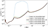 |
Fig. B.1. Profiles of the vertically conductivity-averaged resistivity, |

Vertical temperature profile: Our hydrodynamical equations Eqs. (1) - (4) are formulated in using an isothermal vertical disk structure. Recent studies by e.g. Jankovic et al. (2021) show that the vertical temperature structure in the inner disk is highly dependent on viscous heating and therefore is also dependent on the vertical density structure, but should also be dependent on heating via non-thermal ionisation, making upper layers hotter than the midplane. Hence, the calculation of the ionisation degree by taking the midplane gas temperature, Tgas, 0, and using it as the vertically isothermal gas temperature at every height z would vastly overestimate the vertical extent of the thermally ionised disk region. We therefore used a physically motivated vertical gas temperature profile (see Eq. (70), for the physical background, see e.g. Hubeny 1990). The thermally ionised region in our models agrees reasonably well in both the radial and vertical extent with the vertically self-consistent 2D models of Jankovic et al. (2021) and are therefore valid to describe the thermally ionised region. With regard to the discrepancy between the use of an isothermal vertical disk for hydrodynamical simulations while applying a vertical temperature profile for calculating the thermal ionisation degree, we argue as follows: The vertical disk structure (apart from the magnetic field) is described in a 1+1D simulation by density-weighted variables (e.g. Σ, Pgas). Therefore, the disk region around the midplane dominantly contributes to describing the vertical disk structure, which justifies using Tgas, 0 as the temperature of an isothermal vertical disk when performing hydrodynamical simulations.
All Tables
Dust recombination rate for the dust grain size ad = 0.1 μm and different gas temperature regimes.
All Figures
|
Fig. 1. Time evolution of the magnetic field strength over time (normalised in units of the diffusion timescale of the stationary model at the outer DZ boundary, tdiff, stat(rDZ, out)), where the colour-coding represents the magnetic field strength, |B|, at every point in space and time. The gray lines show magnetic flux transport over time, using the effective, vertically averaged magnetic field transport velocity, |
| In the text | |
|
Fig. 2. Timescales of our reference model (cf. Table 2) relevant to the long-term evolution of a PPD and a large-scale magnetic field. The solid blue, orange, and green lines correspond to the viscous timescale, tvisc; the dynamical timescale, tdyn; and the magnetic diffusion timescale, tdiff, respectively. The vertical, dashed black lines correspond to the corotation radius, Rcor, and the outer DZ boundary, rDZ, out. Finally, the gray area marks the region between 1 Myr and 4 Myrs and depicts the expected lifetime of a PPD. |
| In the text | |
|
Fig. 3. Poloidal stationary magnetic field profile of our reference model (see Table 2). Panel (a) shows both the vertical and radial magnetic field component at the surface, Bz and Brs, respectively. Panel (b) depicts the ratio of Brs/Bz, which is a measure for the inclination of the field lines, whereas panel (c) shows the magnetic plasma beta β0 at the disk midplane. The vertical dashed line correspond to the corotation radius, Rcor, and rDZ, out, respectively. The dotted, gray lines in panels (a) and (c) describe the corresponding values at t = 0, whereas the horizontal dotted line in panel (b) denotes a surface angle of 30° with respect to the midplane normal. |
| In the text | |
|
Fig. 4. Comparison of the viscous timescale, tvisc, and the diffusion timescale, (tdiff, stat). The vertical dashed lines close to the inner rim and at ∼4 AU represent Rcor and rDZ, out, respectively. |
| In the text | |
|
Fig. 5. For better understanding of the regimes of thermal and non-thermal ionisation, the radial and vertical profiles of (a) ionisation fraction, xe; (b) the contribution of OD, ηO; (c) the contribution of AD, ηA; and (d) the combined resistivity, η(r, z) = ηO(r, z)+ηA(r, z), are plotted for our reference model, which is explained in Sect. 3.1 (cf. Table 2). The dashed gray lines in (a)–(d) correspond to specific heights above the disk midplane (z = 0, z = Hp, |
| In the text | |
|
Fig. 6. Panel (a), energy contributions to the overall inner energy budget for every disk annulus at radius r. Q : ∇u, Γ − Λ, Pgas ∇⋅u, 4 π Σ κR(J − S), and Ėadv, denote energy rates per unit volume due to viscous heating, heating or cooling over the surface, work done by gas pressure per unit time, radial radiation flux, and net inner energy advection, respectively (see Eq. (3)). Panel (b), plot of the midplane gas temperature, Tgas, 0. The vertical dashed line in all panels denotes the corotation radius, Rcor, and the gray area marks the optically thin region in the inner disk. |
| In the text | |
|
Fig. 7. Comparison of the magnetic field topology between our reference model (P⋆ = 4 days, black) and two stars with P⋆ = 5 days (blue) and P⋆ = 6 days (orange). The vertical dashed lines mark the positions of Rcor and are colour-coded accordingly. Panels (a) and (b) show the vertical and radial magnetic field profiles in the inner and outer disk, respectively. Panels (c) and (d) depict the conductivity-weighted, vertically averaged resistivity |
| In the text | |
|
Fig. 8. Same as Fig. 7 but for different values of |B⋆|. The stellar field strengths, |B⋆|, of 1 kG, 500 G, and 200 G respectively correspond to the black, blue, and orange lines. |
| In the text | |
|
Fig. 9. Same as in Fig. 7 but for different stellar X-ray luminosities, LX, reaching from 1029 erg s−1 to 1031 erg s−1. |
| In the text | |
|
Fig. 10. Same as in Fig. 7 but for different Ṁ. The colour-coded vertical dashed lines correspond to the outer dead zone boundaries, rDZ, out, of the respective disk model. |
| In the text | |
|
Fig. 11. Magnetocentrifugal winds mass loss, Ṁwind, according to Eq. (86) for our reference model (black). All other models discussed in this paper are shown as light grey lines to further illustrate the two dominant wind regimes in the innermost disk and in the outer disk. |
| In the text | |
|
Fig. 12. Stationary magnetic field topology for different initial fossil field strengths. The reference model uses a fossil field with β0 = 102 (black) and is compared to two models with a stronger initial field (β0 = 10 (blue) and β0 = 1 (orange)). The panels are the same as in Fig. 8. The vertical dashed lines correspond to Rcor and rDZ, out. |
| In the text | |
|
Fig. B.1. Profiles of the vertically conductivity-averaged resistivity, |
| In the text | |
Current usage metrics show cumulative count of Article Views (full-text article views including HTML views, PDF and ePub downloads, according to the available data) and Abstracts Views on Vision4Press platform.
Data correspond to usage on the plateform after 2015. The current usage metrics is available 48-96 hours after online publication and is updated daily on week days.
Initial download of the metrics may take a while.