| Issue |
A&A
Volume 703, November 2025
|
|
|---|---|---|
| Article Number | A5 | |
| Number of page(s) | 26 | |
| Section | Extragalactic astronomy | |
| DOI | https://doi.org/10.1051/0004-6361/202554972 | |
| Published online | 31 October 2025 | |
Re-assessing the stellar population scaling relations of the galaxies in the Local Universe
1
Dipartimento di Fisica, Università di Trento, Via Sommarive 14, I-38123 Povo (TN), Italy
2
INAF-Osservatorio Astrofisico di Arcetri, Largo Enrico Fermi 5, I-50125 Firenze, Italy
3
Dipartimento di Fisica e Astronomia, Università degli Studi di Firenze, Via G. Sansone 1, I-50019 Sesto Fiorentino, Italy
⋆ Corresponding author: This email address is being protected from spambots. You need JavaScript enabled to view it.
; This email address is being protected from spambots. You need JavaScript enabled to view it.
Received:
1
April
2025
Accepted:
13
August
2025
Abstract
Context. Local galaxies follow scaling relations between their mass and stellar population properties, such as age and metallicity. These relations encode fundamental information about the past evolutionary history of galaxies.
Aims. We want to revise stellar population scaling relations of local galaxies by leveraging the largest spectroscopic dataset provided by Data Release Seven of the Sloan Digital Sky Survey (SDSS DR7) at 0.005 < z < 0.22, using improved stellar population synthesis (SPS) models and novel SDSS aperture bias corrections.
Methods. We applied statistical weights to account for selection biases and implemented corrections to the SDSS fibre aperture limitations. Within a Bayesian framework, we estimated the stellar masses, mean stellar ages, and mean stellar metallicities by comparing the spectral indices and photometry with composite stellar population models. We adopted state-of-the-art ingredients and updated prescriptions to better capture the complexity of galaxies star formation and chemical enrichment histories. We also tested different models and priors.
Results. We estimated light-weighted mean stellar ages for 354 977 galaxies (S/N ≥ 10) and metallicities for 89 852 galaxies (S/N ≥ 20), and studied their dependence on stellar mass. Our key findings include: i) a revised bimodal distribution in the mass-age plane, with a young sequence (dominant at low masses) and an old sequence (dominant at high masses), partly overlapping in mass and transitioning at Mtr = 1010.80 M⊙; ii) a mass-metallicity relation (MZR) shifted ∼0.2 dex higher than in previous studies. Our aperture corrections produce mass-dependent reductions in masses, ages, and metallicities, enhancing the young sequence and steepening the MZR at low masses; iii) using Hα-based star formation rate classification, we found that while star-forming+young and quiescent+old correspondences generally hold, some exceptions exist for many galaxies. Quiescent galaxies show flatter, less scattered MZR than star-forming ones, converging at high masses; and, finally, iv) different SPS modelling assumptions significantly impact results, with star formation and chemical enrichment histories having the strongest effects.
Conclusions. These revised relations provide new benchmarks for galaxy evolution studies and simulations. Systematic effects of 0.1 − 0.2 dex can arise from uncorrected aperture biases and different SPS modelling choices. Consistent assumptions should be applied when comparing observations and models.
Key words: galaxies: evolution / galaxies: fundamental parameters / galaxies: general / galaxies: statistics / galaxies: stellar content
© The Authors 2025
 Open Access article, published by EDP Sciences, under the terms of the Creative Commons Attribution License (https://creativecommons.org/licenses/by/4.0), which permits unrestricted use, distribution, and reproduction in any medium, provided the original work is properly cited.
This article is published in open access under the Subscribe to Open model. This email address is being protected from spambots. You need JavaScript enabled to view it. to support open access publication.
1. Introduction
The observed properties of galaxies in the Local Universe are connected through well-known scaling relations, which are fundamental tools for investigating how galaxies form and evolve. The scaling relations that connect the stellar mass of the galaxies with the ages and metallicities of the stellar population that compose them are of particular relevance, as stellar populations retain a wealth of ‘archaeological’ information about past star formation and chemical enrichments histories. Traditionally the study of these relations was accessible only in the context of quiescent elliptical galaxies (e.g. Tinsley & Gunn 1976; Tinsley 1980; Bruzual 1983; Gonzalez et al. 1993; Kauffmann 1996). The advent of more refined models for stellar population synthesis (SPS; e.g. Bruzual & Charlot 2003) meant that these relations could be characterised for galaxies with any star formation activity. Higher resolution spectroscopic surveys such as Sloan Digital Sky Survey (SDSS; York et al. 2000; Stoughton et al. 2002) enabled the estimation of stellar ages and metallicities, as well as their relations with galaxy stellar mass, for a large number of galaxies in the Local Universe (e.g. Kauffmann et al. 2003a,b; Panter et al. 2003, 2008; Tremonti et al. 2004; Gallazzi et al. 2005, 2008, 2021; Cid Fernandes et al. 2007; Vale Asari et al. 2009; Mannucci et al. 2010; Pasquali et al. 2010; Peng et al. 2015; Trussler et al. 2020; Sánchez et al. 2018; Sánchez 2020). These relations showed the existence of a bimodal mass-age relation composed by two distinct sequences of young low-mass and old high-mass galaxies (see also Mateus et al. 2006). A smooth transition between the two sequences occurs at a stellar mass of M⋆ ∼ 1010.5 M⊙ ∼ 3 ⋅ 1010 M⊙ (Kauffmann et al. 2003a; Gallazzi et al. 2005; Moustakas et al. 2013; Haines et al. 2017). In addition to the mass-age relation, galaxies also exhibit a strong connection between stellar mass and stellar metallicity, known as the mass-(stellar) metallicity relation (MZR). The stellar MZR of galaxies in the Local Universe has a unimodal shape with increasing stellar metallicities for increasing masses, flattening in the high mass end. These relations have been used in the local Universe to characterise galaxy evolution within a downsizing scenario (Gallazzi et al. 2005; Panter et al. 2008; Fontanot et al. 2009; Thomas et al. 2010). In this context, higher mass galaxies (on average, older and more metal-rich) efficiently formed stars at earlier cosmic epochs, resulting in shorter formation timescales and higher enrichment efficiencies. On the contrary lower-mass galaxies reached the peak of their star formation activity more recently, resulting in longer formation timescales and lower chemical enrichment efficiencies.
In recent decades, models of galaxy formation and evolution in a cosmological context have been proven capable of reproducing several observational properties of Local Universe galaxies in a realistic way (see the review by Somerville & Davé 2015, and references therein). These models enable us to formulate a realistic representation of Local Universe galaxies, in addition to predicting the properties of galaxies at higher redshifts. Local Universe scaling relations are fundamental observational constraints to the treatment of the different astrophysical mechanisms governing galaxy growth in theoretical models of galaxy formation.
Modern models of galaxy formation and evolution are built upon a number of scaling relations, which have been characterised in the Local Universe primarily thanks to extensive spectroscopic surveys. The SDSS is the largest statistical database to-date used to study galaxy scaling relations. However, we know that SDSS spectroscopic measurements suffer from an observational bias due to the limited aperture of the optical fibres used to extract galaxies spectra, which is generally referred to as an ‘aperture effect’ (e.g. Kauffmann et al. 2003a; Gallazzi et al. 2005, 2008; Peng et al. 2015; Trussler et al. 2020; Gallazzi et al. 2021). In fact, galaxy spectra in the SDSS are extracted using optical fibres centred on the centre of the target galaxy and collecting light from a circular region with a diameter of 3″. Since a galaxy’s apparent size depends on both its physical dimensions and distance, the fibre coverage varies across different galaxies. This leads to a non-uniform loss of light from the outer regions of observed galaxies. In addition to this bias, models and inference methods may introduce systematic biases in the estimates of stellar population parameters. The combination of observational and systematic biases can result in uncertainties in the scaling relations which, in turn, could give rise to systematics when making comparisons with model predictions or different datasets.
In recent years, the advent of IFU surveys such as MaNGA (Bundy et al. 2014) and CALIFA (Sánchez et al. 2012) has enabled the study of galaxies in the Local Universe on spatially resolved scales (see Sánchez 2020, for a review). As a result, we have been able to quantify the spatial variations and gradients of stellar population properties (e.g. Pérez et al. 2013; Sánchez-Blázquez et al. 2014; González Delgado et al. 2014, 2015; Goddard et al. 2017; Zibetti et al. 2017, 2020; Zibetti & Gallazzi 2022; Martín-Navarro et al. 2018; Li et al. 2018; Johnston et al. 2022). Most recently, Zibetti et al. (2025) leveraged the spatial information and extensive coverage of the CALIFA dataset to statistically characterise and correct the aperture biases in the SDSS spectroscopy.
Taking advantage of these corrections, together with the advancements in population synthesis models, we built upon the work of Gallazzi et al. (2005) to revise the mass-age and mass-stellar metallicity scaling relations in the Local Universe. Specifically, we have improved on the previous work in the following ways: 1) on the observation side, we applied correction factors to account for the aperture effects in the absorption indices estimates; 2) on the modelling and stellar population parameter side, we used updated simple stellar populations (SSP), obtained with state-of-the-art modelling (2019 version of Bruzual & Charlot 2003) and we introduced more refined prescriptions for the star formation histories (SFHs; Sandage 1986; Asari et al. 2007; Pacifici et al. 2016), chemical enrichment histories (CEHs; Erb 2008; Zibetti et al. 2017; Camps-Fariña et al. 2021, 2022), and dust absorption (Charlot & Fall 2000). Furthermore, we also implemented statistical weights accounting for Malmquist (Schmidt 1968) and sample selection biases. Based on this work, we now present volume-weighted aperture-corrected scaling relations obtained with state-of-the-art SPS models, exploiting the large statistics provided by the SDSS Data Release 7 (DR7) sample.
Our revised scaling relations provide a new reference that can be used by theoretical models to constrain the processes shaping galaxy evolution (e.g. galaxy quenching; e.g. Peng et al. 2015; Casado et al. 2015; Spitoni et al. 2017; Trussler et al. 2020; Bluck et al. 2020a,b; Corcho-Caballero et al. 2023a,b; Looser et al. 2024) and fine-tune the corresponding parameters; it also sets a local benchmark for higher redshift scaling relations (e.g. Gallazzi et al. 2014; Cappellari 2023; Nersesian et al. 2024; Gallazzi et al. 2025a,b). This is particularly meaningful given the advent of next-generation surveys such as WEAVE-StePS (Iovino et al. 2023b) and 4MOST-StePS (Iovino et al. 2023a), which will provide deep spectroscopy of large near-mass selected samples. These advances will allow us to bridge the redshift gap between SDSS at z ∼ 0 and LEGA-C (van der Wel et al. 2016) at 0.6 < z < 1, enabling a uniform characterisation of stellar populations.
The paper is organised as follows. In Sect. 2, we present the dataset used throughout this work and describe the methodology used to estimate the statistical weights accounting for observational and selection biases. In Sect. 3, we describe the procedure to retrieve the galaxy properties from the observed spectra, focussing also on the analysis of the individual ingredients of the SPS modelling. In Sect. 4, we present our revised mass-age and mass-stellar metallicity relations for galaxies in the Local Universe, both for the general population and considering passive and star-forming galaxies separately. In Sect. 5, we analyse the systematics induced in the scaling relations by different choices for the ingredients of the SPS models, with a detailed analysis of the differences with respect to previous works from our group and, specifically, to Gallazzi et al. (2005) and Gallazzi et al. (2021). We discuss the importance of these revised and bias-corrected relations in the context of galaxy evolution in Sect. 6. We summarise our results and conclusions in Sect. 7. Throughout the paper, we assume a ΛCDM cosmology with H0 = 70 km s−1 Mpc−1, Ωm = 0.3, and ΩΛ = 0.7.
2. Data analysis
In this section, we describe the sample and dataset used in this work. We also describe the process followed to obtain statistical corrections for biases due to sample selection and aperture effects.
2.1. Observational dataset
The dataset used in this work is composed of both photometric and spectroscopic observations drawn from the SDSS DR7 (Abazajian et al. 2009). The SDSS (York et al. 2000; Stoughton et al. 2002) is an optical photometric and spectroscopic survey conducted using a 2.5 m telescope at Apache Point Observatory, in Southern New Mexico. The photometry is obtained in the five bands ugriz (Fukugita et al. 1996), using a mosaic CCD camera (Gunn et al. 1998). Spectroscopic observations are carried out using 640 optical fibres with 3″ diameter apertures. The spectra cover the wavelength range 3800−9200 Å, with an average spectral resolution R = λ/Δλ ∼ 2000. The DR7 delivers photometry of 375 million objects and spectroscopy of ∼1.6 million objects (Abazajian et al. 2009), including ∼930 000 galaxies.
The observational features we used to estimate galaxy properties are a set of absorption indices, which can be extracted from the spectra of the galaxies (Worthey et al. 1994; Worthey & Ottaviani 1997), and the SDSS ugriz Petrosian photometry. Given the studies that have characterised the dependence of the absorption indices on the ages and metallicities of galaxies stellar populations (Worthey et al. 1994; Worthey & Ottaviani 1997; Thomas et al. 2003; Bruzual & Charlot 2003), we followed Gallazzi et al. (2005) and used the break at 4000 Å (D4000n). As defined in Balogh et al. (1999), this is a set of three Balmer indices: Hβ, and HδA+HγA, and two composite magnesium and iron indices [MgFe]′, and [Mg2Fe], expressed as
![Mathematical equation: $$ \begin{cases} { \mathrm {[MgFe]}^\prime} =\sqrt{\mathrm {Mgb}\,(0.72\,\mathrm {Fe5270}+0.28\,\mathrm {Fe5335})},\\ \\ {[\mathrm {Mg}_{2\mathrm {Fe}}]} = 0.6\,\mathrm {Mg}_2+0.4\,\log (\mathrm {Fe4531}+\mathrm {Fe5015}), \end{cases} $$](/articles/aa/full_html/2025/11/aa54972-25/aa54972-25-eq1.gif) (1)
(1)
as defined by Thomas et al. (2003) and Bruzual & Charlot (2003). This choice for the absorption indices is driven by the need to reduce the age-metallicity degeneracy. This can be achieved by using mainly age-sensitive indices, such as high-order Balmer lines and the D4000n break, which are synergistic with indices that are mainly metallicity-sensitive, such as [MgFe]′ and [Mg2Fe]. These composite magnesium and iron indices are designed to be good tracers of the overall metallicity and, at the same time, have only a slight dependence on [α/Fe] (Thomas et al. 2003; Bruzual & Charlot 2003). The index measures used in this work were obtained from the emission line-subtracted spectra from Brinchmann et al. (2004) and have been made available from the ‘MPA-JHU catalogues’1.
The MPA-JHU catalogues contain photometric and spectroscopic properties of 927 552 galaxies, some of which are associated to repeated observations of the same galaxy. From this sample, we rejected 48 599 observations due to low quality redshift and velocity dispersion measurement2. We combined the repeated observations and created a catalog of unique observations for each galaxy identified as unique by the photometric pipeline (Lupton et al. 1999). The repeated spectroscopic observations were combined by calculating the error-weighted averages of the galaxy properties that we used in our analysis, namely: redshift, velocity dispersion σ⋆ (used to broaden the spectral features of the models to match the observed ones), star formation rate (SFR, used to separate passive and star-forming galaxies), and index measures (for D4000n, Hβ, HγA, HδA, and the indices needed to compute [MgFe]′, and [Mg2Fe]). For the combination of the repeated absorption index measures, we used only those associated to valid (positive) uncertainties. The photometric information are drawn from the NYU Value-Added Galaxy Catalog by Blanton et al. (2005, NYU-VAGC hereafter3), which we matched with the MPA-JHU following the combination of the duplicated observations, using the nearest neighbour method, based on the sky coordinates. We thus obtained a catalog of science-grade and unique observations for the full SDSS DR7 galaxy sample, containing 825 263 galaxies.
We then selected galaxies that constitute a suitable sample for the stellar population analysis. We selected only galaxies that are part of the Main Galaxy Sample; hence, those with 14.5 ≤ rpetro, dered ≤ 17.77 mag (Strauss et al. 2002)4. We also restricted the sample to galaxies in the redshift range 0.005 < z ≤ 0.22. Galaxies with z ≤ 0.005 are excluded in order to avoid bad distance determinations due to deviations from the Hubble flow; galaxies with z > 0.22 were excluded because of severe mass incompleteness given the apparent magnitude limits of the SDSS. We also rejected galaxies with velocity dispersion exceeding 375 km/s to exclude possible non-physical measurements (possibly large errors). Rare extreme or peculiar objects might be rejected as well, yet this may be considered acceptable given the statistical nature of this study. We also used the SDSS photometric flags to reject 253 037 galaxies with bad quality photometric measurements5. As at faint absolute magnitudes, the representativeness of our sample drops dramatically (see Sect. 2.2), we rejected galaxies with absolute r-band magnitudes of Mr > −17.56. Gallazzi et al. (2005) showed that a signal-to-noise ratio (S/N) per pixel of at least 10 and 20 are needed to get reliable estimates of ages and metallicities, respectively (see also Rossi 2025). For this reason, we also imposed S/N cuts to select suitable galaxies to perform the analysis on mass-age and mass-metallicity scaling relations separately. After the combination of the duplicated observations and the sample selections we are left with 354 977 galaxies with S/N ≥ 10, and 89 852 galaxies with S/N ≥ 20.
2.2. Corrections for statistical biases
The apparent-magnitude cut that defines our sample implies that our sample is not volume-complete. We corrected for such incompleteness by calculating statistical volume weights following Schmidt (1968). Based on the Petrosian magnitudes in the NYU-VAGC catalog, we computed the minimum and maximum redshifts, namely, zmin and zmax, at which each galaxy enters the selection cuts, taking into account the K-corrections computed with the Kcorrect code by Blanton & Roweis (2007). The ratio between the comoving volume ΔVsurv = V(z = 0.22)−V(z = 0.005) within the redshift boundaries of our sample selection and the comoving volume ΔVmax = V(zmax)−V(zmin) within zmin and zmax gives the statistical weight of each galaxy to account for the Malmquist bias.
Incompleteness due to fibre allocation, data quality rejection, and S/N selection can also induce biases in how the selected sample is representative of the underlying parent population. To correct for such effects, we calculated statistical weights based on the unbiased photometric NYU-VAGC catalogue. We calculated completeness corrections for each S/N selection by comparing the 2D distribution of the complete NYU-VAGC sample and of our samples in the  plane, obtained using the absolute magnitudes K-corrected at redshift z = 0.1. We estimated the completeness fractions, κ, by calculating the ratio between the NYU-VAGC number-density distribution and the one obtained with our sample. Adopting, for each galaxy, the statistical weight
  , we can thus obtain a volume-complete statistical representation of the galaxy population.
To reproduce the volume density of galaxies, we multiplied the statistical weights by the factor N = 4.89 × 10⁻⁹ h3Mpc−3, which we can use to exactly reproduce the Blanton et al. (2003) luminosity function in the magnitude range −22 < 0.1Mr < −21. Figure 1 illustrates the statistical corrections both for the volume and completeness effects, as well as the resulting distribution in the colour-magnitude diagram (CMD) for the galaxies with S/N ≥ 10 (similar plots are obtained for S/N ≥ 20). The top panels show the 2D maps of  and κ (left and right panels, respectively). Volume corrections depend essentially on the absolute magnitude alone, resulting in a gradient along the x-axis, with fainter galaxies having the strongest corrections. As we can see from Fig. 1, moving towards faint absolute magnitudes (and blue colours), the overall representativeness drops below 10−3. To avoid overwhelming our analysis with galaxies with very high statistical noise, we limited the study of scaling relations to galaxies with Mr < −17.5, as mentioned above.
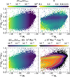 |
Fig. 1. CMD for the galaxy sample with S/N ≥ 10. Top-left: Volume completeness (i.e. the inverse of the volume-weights). Top-right: Completeness fractions (i.e. the inverse of the completeness-weights). Bottom-left panel: Statistical weights obtained combining the volume and completeness statistical weights, multiplied by the factor N = 4.89 × 10⁻⁹h3 Mpc−3, to convert number counts to the number volume-density of galaxies. Bottom-right: Number density of galaxies in the CMD applying the completeness corrections. The green contours enclose 16%, 50%, 84%, and 97.5% of the galaxy sample, and have been obtained on the distribution smoothed with a Gaussian KDE. Similar plots are applicable to the S/N ≥ 20 sample. |
On the other hand, the completeness fractions depend both on the magnitude and the colour of the galaxies. The highest completeness fraction κ ∼ 0.65 is reached by galaxies with (0.1Mg− 0.1Mr) ∼ 0.75. Bluer galaxies have progressively lower completeness fractions reaching κ ∼ 0.1 at the faint end and bluest colour. The bottom-left panel shows the 2D map of the overall statistical corrections (in units of  ) obtained by multiplying the completeness correction by the volume correction times the conversion factor, N. We note the dependence on both colour and magnitude, inherited from the completeness corrections. The bottom right panel shows the number density of galaxies when implementing the overall statistical weights. The green contours identify the density levels enclosing 16%, 50%, 84%, and 97.5% of the complete galaxy sample. Such contours were derived by smoothing the distribution using a Gaussian kernel density estimator (KDE).
As a sanity check on the robustness of our statistical weights, throughout the work we have verified that the weighted distributions obtained from the S/N ≥ 10 sample are consistent with the ones obtained from the more restricted sample at S/N ≥ 20, except for the noise attributed to the varied number statistics. The mass functions shown in Fig. 10 illustrate this. A posteriori, we can claim that our galaxy sample is representative for galaxy masses as low as ∼109 M⊙ overall, and down to ∼109.5 M⊙ for passive and old galaxies (which are a minority at the low-mass end). These limits can be graphically identified in Fig. 10 as the masses for which the mass functions display a sharp down-bending, also indicated by the shaded areas.
2.3. Corrections to indices for fibre aperture bias
The SDSS optical fibres were positioned on the centre of the target galaxies and collected light from a circular region with a diameter of 3″(i.e. only from a central portion of a galaxy’s extent). Since a galaxy’s apparent size depends both on its physical dimensions and on distance, the fibre coverage varies across different galaxies. This leads to a non-uniform loss of light from their outer regions. Several studies showed that galaxies may present significant radial gradients in their stellar populations properties (e.g. based on IFU observations, González Delgado et al. 2014, 2015; Goddard et al. 2017; Li et al. 2018; Zibetti et al. 2017, 2020; Zibetti & Gallazzi 2022). Also, galaxies physical properties may change in different galaxy components. For instance, it is known that bulges are typically composed primarily of old and metal-rich stellar populations, with low-level or absent star formation. On the contrary, discs display a variety of populations both in age and metallicity. The strength of stellar population gradients in galaxies thus depends on the properties and dominance of each component, hence on morphology and, in turn, on mass. The combination of the non-uniform galaxy coverage from SDSS fibres, together with the presence of radial gradients in stellar population properties, causes a systematic observational bias, which we refer to as ‘aperture effects’ in the following.
Zibetti et al. (2025) calculated the corrections to the absorption indices measured on SDSS spectra needed to obtain the indices relative to the full integrated light of the galaxy. The authors used integral field observations from CALIFA to simulate the effect of a fixed 3″ aperture on the measurement of absorption indices from galaxies with different masses and morphologies. The aperture-corrections were divided into first- and second-order offsets, which are assigned to each galaxy based on its position in the index-strength vs. (g − r) and r50 vs. Mr, petro planes. We used the indices measures and the half-light radii (with the respective errors) obtained from theMPA-JHU catalogue (converting the r50 from arcsecond to kpc using the angular diameter distance estimated with the MPA-JHU redshift). The absolute magnitudes, Mpetro, and (g − r) colours were obtained from the NYU-VAGC, using the Petrosian values.
The effects of the aperture corrections and of the statistical weights are illustrated in the distributions of the observed galaxies in the HδA+HγA vs. D4000n and HδA+HγA vs. [MgFe]′ planes, in Fig. 2 (top and bottom row, respectively). These index-index planes are diagnostic for the stellar population age and metallicity, respectively (Gallazzi et al. 2005, 2014). The left panels display the distribution prior to applying either statistical weights or aperture corrections. The central panels display the galaxy density distribution obtained applying the statistical corrections for volume and completeness. The right panels present the fully corrected distributions, after applying the aperture corrections to the index measurements and the statistical weights. The aperture corrections substantially enhance the galaxies populating the parts of the planes associated to high values of HδA+HγA and low values of both D4000n and [MgFe]′. Since D4000n and [MgFe]′ are proxies for ages and metallicities respectively, this results in an enhancement of the galaxies with young and metal poor stellar populations. Furthermore, the aperture corrections reduce the scatter of the 2D distributions in both HδA+HγA vs. D4000n and HδA+HγA vs. [MgFe]′ planes, as analysed in more detail in Zibetti et al. (2025).
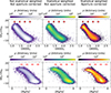 |
Fig. 2. Distribution of the galaxies in the HδA+HγA vs. D4000n and HδA+HγA vs. [MgFe]′ planes before and after the implementation of the statistical weights and the aperture corrections. Left panels: Distribution of the original data, i.e. simple number counts for uncorrected index values. Central panels: Distributions of galaxies weighted by the volume and completeness statistical corrections, for uncorrected index values. Right panels: Distributions obtained by implementing both the statistical weights and the corrections for aperture effects. The error bars correspond to the median uncertainties calculated in four bins of D4000n and [MgFe]′, for samples with S/N ≥ 20 (red) and S/N ≥ 10 (shown in black at the top). |
3. Methodology
In this section we describe the methodology used to perform the inference of the stellar population parameters, detailing the ingredients used in the SPS study.
3.1. Bayesian inference of stellar population properties
We estimated the galaxy stellar population properties by means of the Bayesian Stellar population Analysis (BaStA) tool, developed by A. Gallazzi and S. Zibetti and presented in several previous works by our group (e.g. Gallazzi et al. 2005; Zibetti et al. 2017). Here, we provide a brief overview of its operating principles. The key idea is to derive the posterior probability distribution function (PDF) of a given stellar population parameter using a Bayesian approach in which the prior PDF is defined by a pre-computed library of SPS models (following the approach of Kauffmann et al. 2003a; Gallazzi et al. 2005; da Cunha et al. 2008). In our case, the prior distribution is composed by a library of 500 000 composite stellar populations (CSPs). Taking each model spectrum, generated by prior assumptions in SFH, CEH, and dust (see Sect. 3.2), we can associate physical parameters (e.g. mean stellar age and metallicity) and observational parameters (e.g. photometry and absorption indices measurements) to them. Therefore, given an observed dataset for a galaxy, for each SPS model, we define the likelihood given the data as
 (2)
(2)
where O and σ are the measurements and uncertainties of the observed quantities, while M refers to the corresponding quantities predicted by the given model. For each physical parameter, we then obtain its posterior PDF by marginalising over all other properties. From this, we estimated the fiducial value of the parameter as the median, with its uncertainty given by half the range between the 16th and 84th percentiles. As observational constraints, we used the five indices and the five photometric fluxes defined in Sect. 2.1. The observed indices are confronted with the model indices computed for a velocity dispersion broadening consistent with the observed one7.
We applied this Bayesian approach to infer the light-weighted and (present-day) mass-weighted ages and metallicities, as defined in Equations 3 and 4, respectively,
 (3)
(3)
 (4)
(4)
where t measures the time along the SFH, t0 is the time elapsed since the start of the SFH until the epoch of observation, SFR(t) is the star formation rate as a function of time, ℒ′(t) is the luminosity arising per unit of formed stellar mass from the SSPs of age t0 − t, and R(t) is the fraction of stellar mass returned to the inter-stellar medium (ISM).
Since mass is an extensive property, it cannot be directly extracted from the models. For each model we compute the normalisation factor that has to be applied to the model photometric fluxes in order to match the observed ones. This is done by minimizing the χ2 corresponding to the magnitudes in the five SDSS bands. Since by construction all models are normalised to 1 M⊙ in present day stellar mass (including living stars and stellar remnants), this normalisation factor directly gives the present day stellar mass in units of solar masses for a given model. This parameter is then treated as the other physical parameters in the marginalisation of the posterior PDF.
3.2. The stellar population model library
In this section, we provide an essential description of how the library of CSPs that constitute the prior for our Bayesian inference was constructed. More technical details can be found in Appendix A. In this work we adopted the grid of SSPs from the 2019 version of the Bruzual & Charlot (2003, CB19 hereafter)8. Such SSPs assume a Chabrier (2003) initial mass function (IMF) with a maximum M⋆ = 100 M⊙, use the MILES spectral libraries (Sánchez-Blázquez et al. 2006), and model stellar evolution via the PARSEC (Bressan et al. 2012; Marigo et al. 2013; Chen et al. 2015) evolutionary tracks (for a more detailed description of the CB19 ingredients, we refer to Appendix A of Sánchez et al. 2022).
We synthesised the CSPs combining SSPs based on parametric SHFs and CEHs. The emergent spectra are then attenuated according to a dust attenuation model. We used SFHs composed by a continuum parametric component superimposed with random bursts of star formation, to incorporate stochasticity. For the continuum component we implemented a delayed Gaussian SFH, following Sandage (1986) and Gavazzi et al. (2002):
 (5)
(5)
with the timescale, τ. This formalism allows for more flexibility in the description of a galaxy SFH, with respect to a decaying exponential law (adopted in several studies, including, e.g. Gallazzi et al. 2005), by including an increasing phase, which may reveal more appropriate for the early phase of galaxy evolution or even the present-day evolution of low-mass galaxies (Asari et al. 2007; Pacifici et al. 2016). The look-back time of the beginning of the SFH tform, lb ≡ t0 − tform (t0 being cosmic time of the observation) is chosen randomly between 500 Myr and 20 Gyr9, from a uniform logarithmic distribution. The parameter τ (time of the maximum SFR since the beginning of the SFH and time-scale of the Gaussian decay) is randomly generated ranging from 1/20 to 2 times tform, lb. The smallest τ/tform, lb correspond very closely to SSPs of age equal to tform, lb (see also Zibetti et al. 2024).
The burst-like component is composed by one or more bursts of star formation (up to six), and affects two thirds of the models. The probability to have Nburst is proportional to exp−Nburst. Each burst can form between 10−3 and 2 times the total mass formed in the continuos component. The age of each burst can vary from 105 yr to tform, lb. Although not explicitly modelled, different combinations of a secular component with τ ≪ tform, lb and recent burst(s) can reproduce post-starburst galaxies or truncations of the SFH.
Our CSPs were constructed using the parametric CEHs defined in Zibetti et al. (2017):
 (6)
(6)
where M(t) and Mfinal are the stellar mass formed at time t and the total stellar mass formed until the end of the SFH respectively, and α ≥ 0 is a parameter that describes how fast the chemical enrichment proceeds relative to the formation of stars and can vary between 0.25 and 19. In case of the presence of bursts in the SFH, at each burst is assigned a metallicity Z⋆ burst equal to the metallicity of stars formed in the continuous mode at time of the burst, plus a random offset taken from a log-normal distribution with σ = 0.2 dex.
It should be noted that the leaky-box model CEH defined in Eq. (6) (see also Erb 2008) does not allow for possible decreases in Z⋆ due to, for instance, the infall of metal poor gas from the inter-galactic medium (IGM), and the consequent dilution of the gas reservoir of the galaxy. These kinds of phenomena are rendered, at least in part, by the down-scatter in the Z⋆ burst with respect to the secular component. We note that the increasing behaviour of the stellar metallicity over time is empirically confirmed to be predominant on average among galaxies (e.g. Camps-Fariña et al. 2021, 2022).
We implemented dust attenuation via the Charlot & Fall (2000) two component model. This model considers different attenuation laws for the diffuse ISM and the dust in the Birth Clouds (BC), with attenuation proportional to λ−0.7 and λ−1.3 respectively. Since young stars (i.e. with Age ≤ 107 yr) reside in the BCs, they suffer attenuation by both components. Young stars are affected by a total optical depth in the V-band of τV, with a fraction μ attributed to the diffuse ISM, and a fraction 1 − μ attributed to the BC. Older stars are effectively attenuated only by the diffuse ISM, hence with a V-band optical depth of μτV. τV and μ are generated using the same prior PDF as in da Cunha et al. (2008) (see also Zibetti et al. 2017).
As detailed in Appendix A, the final model library is produced after applying an equalisation in (HδA+HγA, D4000n), in order to make the model density constant in this plane of observable quantities. Moreover, in the actual procedure of posterior marginalisation, we assign zero weight to models with tform, lb < 1.5 Gyr, which appear to be unrealistic for galaxies with M⋆ ≳ 109 M⊙ in the local Universe. This leaves us with 400 481 effective models.
4. Results
Using the inference method described in Sect. 3 we estimated properties for the galaxy sample both implementing and not-implementing the aperture corrections. In this section, we present and analyse the distributions of galaxies in the mass-age and mass-stellar metallicity planes, taking into account volume and completeness statistical corrections (as calculated in Sect. 2.2). We characterise the stellar populations scaling relations that emerge from these distributions. By comparing the relations obtained from the fiducial aperture-corrected parameters with those without the implementation of aperture corrections we show that these cause significant changes in the scaling relations. Finally, based on existent aperture-corrected estimates of the SFR, we analyse the scaling relations for passive and star-forming galaxies separately.
4.1. Local Universe mass-age and mass-metallicity scaling relations
The central panels of Fig. 3 display the number density distributions of galaxies in the local Universe in the planes defined by light-weighted mean stellar age (Agewr) versus stellar mass (top row) and by light-weighted mean stellar metallicity (Zwr) versus stellar mass (bottom row), based on the parameters obtained with the aperture-corrected indices. The left panels display the same relations obtained without the implementation of the aperture correction. The right panels display the scaling relations for the aperture-corrected mass-weighted mean ages and metallicities, which will be analysed at the end of this section. If not specified otherwise, age and metallicity are meant as light-weighted means in the following. In each mass-age plane the contours identify the isodensity levels enclosing 16%, 50%, 84%, and 97.5% of the complete galaxy sample, calculated from the respective distribution smoothed with a gaussian KDE. In each mass-metallicity plane the solid and dashed lines represent the median and 16th and 84th percentiles of the metallicity distribution as a function of mass, respectively. The red and blue lines in the light-weighed mass-age planes identify the separation between young and old galaxies, which will be defined in Sect. 4.2.
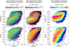 |
Fig. 3. Number density of galaxies for the SDSS DR7 in the mass-age and mass-metallicity planes, obtained using both the volume and completeness statistical weights. Left and central panels: Distributions obtained with light-weighted mean ages and metallicities, without the implementation of aperture corrections (left panels) and implementing aperture corrections (central panels). Right panels: Distributions obtained with mass-weighted mean ages and metallicities for the aperture-corrected sample. In the mass-age planes, the coloured black, green, and fuchsia lines identify the density levels enclosing 16%, 50%, 84%, and 97.5% of the complete galaxy sample, obtained by smoothing the corresponding distribution using a Gaussian KDE. The red and blue lines, overplotted on the top of the mass-age distributions in the left and central panels, for uncorrected and aperture-corrected estimates, respectively, identify the divisions between young and old galaxies, as defined in Sect. 4.2. In the mass-metallicity planes, the coloured black and green solid and dashed lines identify the median and 16th and 84th percentiles of the corresponding distributions in bins of mass. The red lines overplotted on top of the mass-metallicity distribution identify the median relation from Gallazzi et al. (2005). The dotted horizontal lines indicate the solar metallicity of Z⊙ ≡ 0.02. |
4.1.1. Light-weighted scaling relations
In the aperture-corrected age versus mass plane (upper central panel) we see a general trend of increasing light-weighted ages with increasing galaxy mass. For masses below 1010 M⊙ we note the presence of a prominent population of galaxies with ages around 109.3 yr, and a scarcely populated distribution with Agewr > 1010.5 yr. With increasing galaxy mass this sequence of young galaxies becomes progressively less populated, while a sequence of galaxies with light-weighted ages around 109.75 yr arises. At masses M⋆ ≳ 1011 M⊙ the young sequence vanishes, leaving a population of old and massive galaxies. These results confirm the presence of a mass-age relation as already observed in several studies in the literature (e.g. Kauffmann et al. 2003b; Gallazzi et al. 2005, 2021; Pasquali et al. 2010; Trussler et al. 2020; Zibetti & Gallazzi 2022). We note, however, that our mass-age relation displays a more prominent bimodality, whereby the young and old sequences of galaxies coexist in the mass range 1010 − 1011 M⊙, as also highlighted by the green isodensity contours. In the aperture-corrected metallicity vs. mass plane (bottom central panel) galaxies exhibit a unimodal MZR of increasing stellar metallicity with increasing galaxy mass. We visualised this relation and its scatter by overplotting the median relation and 16th and 84th percentiles of the metallicity distribution as a function of M⋆, identified by the green solid and dashed lines respectively, over the 2D distribution. The MZR relation is steeper and has a wider spread at lower masses, while becoming progressively flatter and narrower with increasing galaxy mass.
When comparing our aperture-corrected mass-age relation with the uncorrected one (upper left panel) we see significant differences. The most striking difference concerns the low mass end, where the uncorrected relation shows a much steeper decrease of the light-weighted ages with decreasing galaxy mass below 109 M⊙. For masses M⋆ ≳ 109 M⊙, the implementation of aperture corrections result in an enhancement of the population of the young sequence with respect to the uncorrected distribution. In the mass-stellar metallicity plane we see that the aperture-corrected MZR is characterised by systematically lower stellar metallicities. We note that this difference is mass dependent, with progressively stronger deviations between the two MZRs with decreasing stellar mass, resulting in a steeper slope for the aperture-corrected estimates.
In conclusion, aperture corrections significantly influence both the mass-age and the mass-stellar metallicity relations. The comparisons indicate that the effect of such corrections is mass dependent. We analyse this dependence in more details in Fig. 4, where we show the median shift of galaxies in the mass-age and mass-metallicity planes due to aperture corrections. Following the same colour-code as in Fig. 3, the left panels show the uncorrected distributions and the right panels show the aperture-corrected ones. Over the uncorrected distributions we plotted the median variations in mass, age and metallicity in each 2D bin, identified by the red arrows. Looking at the mass-age distribution, we see that the aperture corrections cause the largest variations in age to the intermediate-age (Agewr ∼ 109.6 yr) galaxies, which reduce their light weighted age by up to ∼0.15 dex. In general, age variations are negative by a few 0.01 up to 0.1 dex over most of the age-mass plane. The majority of galaxies also suffer of a reduction of their mass estimate by up to ∼0.1 dex. The only exception is represented by the galaxies with M⋆ < 1010 M⊙ and Agewr ≲ 109.3 yr, which display an increase both of the mass and light-weighted age estimates by up to ∼0.1 dex and ∼0.15 dex, respectively. In the mass-metallicity plane we find a mass-dependent decrease of the stellar metallicity, with negligible effects in the high mass end, and shifts down to ∼ − 0.4 dex in the low-mass end.
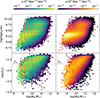 |
Fig. 4. Number density of galaxies for the SDSS DR7 in the mass-age and mass-metallicity planes, obtained using both the volume and completeness statistical corrections. Following the same colour-code of Fig. 3, we give the distributions obtained without aperture corrections (left panels) and the distributions obtained from aperture-corrected indices (right panels). The red arrows (left panels) represent the median shift of galaxies in each bin due to the implementation of aperture corrections. The dotted horizontal lines indicate the solar metallicity of Z⊙ ≡ 0.02. |
4.1.2. Uncertainties of stellar population parameters
Figure 5 displays the aperture-corrected mass-age and mass-metallicity planes, colour-coded by the median uncertainty δ in the mass (left panels), age (central panels), and metallicity (right panels) estimates, respectively, for the S/N ≥ 20 galaxies in each bin on the plane. The green contours identify the isodensity levels as calculated in Fig. 3. The mass-age plane (top panels) shows that mass uncertainties range from ∼0.07 dex to ∼0.17 dex, age uncertainties range from ∼0.15 dex to ∼0.25 dex, and metallicity uncertainties (bottom panels) range from ∼0.1 dex to ∼0.4 dex. We see that both mass and age uncertainties mostly depend on age, while metallicity uncertainties significantly depend both on metallicity and age. The highest mass and age uncertainties pertain to the range 109.3 − 109.8 yr. As we can see in the mass-metallicity planes, mass and age uncertainties depend only marginally on metallicity. On the contrary, metallicity estimates display larger uncertainties for more metal-poor and younger galaxies. In the mass-age diagram we observe a mild trend for less massive galaxies to have larger metallicity uncertainties, which could be the result of the interplay between the mass-age and the mass-metallicity relations. Interestingly, the largest uncertainties in mass and age are found for galaxies with intermediate light-weighted ages (the so-called ‘green valley’ galaxies). This transition range is typically represented by complex SFHs, which are affected by larger degeneracies in the spectral properties. These degeneracies would then be reflected in larger uncertainties on age and, as a consequence, on mass-to-light ratio, hence on stellar mass. Remarkably, metallicity estimates do not appear to be affected by SFH degeneracies. The larger metallicity uncertainties in the metal poor regime derive from the weakness of the absorption features at low metallicity, but are also related to the younger ages that characterise the low-mass metal-poor galaxies.
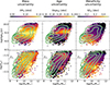 |
Fig. 5. Mass-age (top row) and mass-metallicity (bottom row) distributions of galaxies with S/N ≥ 20, colour-coded by the uncertainties δ in mass (left panels), light-weighted mean age (central panels), and light-weighted mean metallicity (right panels) estimates. The green lines identify the number density levels enclosing 16%, 50%, 84%, and 97.5% of the complete galaxy sample. The dotted horizontal lines indicate the solar metallicity of Z⊙ ≡ 0.02. |
Figure 6 summarises the information about the mass (squares), age (circles), and metallicity (stars) uncertainties as a function of stellar mass. The median errors in mass bins are shown for the three quantities, both for the galaxies with S/N ≥ 10 (empty symbols) and S/N ≥ 20 (filled symbols). We find that age and mass uncertainties attain values of ∼0.19 dex and ∼0.12 dex respectively, not changing significantly when using the sample with higher S/N, as already shown by Gallazzi et al. (2005). This indicates that the reliability of our age and mass estimates is not limited by S/N as long as it is larger than 10, rather by the intrinsic degeneracies of CSP. In fact, we have verified that the distributions in the mass-age planes (weighted by the appropriate statistical factors computed in Sect. 2.2) derived for the S/N ≥ 10 and the S/N ≥ 20 samples are statistically consistent, the only significant difference being the noise due to the different number statistics. When comparing to Gallazzi et al. (2005, see their Fig. 8) we find that our age uncertainties are larger by ∼0.05 dex. This is likely due to the greater variety (and degeneracies) in our CSP models, providing a more extended coverage of the physical parameter space, due to the changes that we implemented in the SPS models (see Sect. 5 for more details).
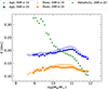 |
Fig. 6. Uncertainties in masses (squares), light-weighted mean stellar ages (circles), and light-weighted mean stellar metallicities (stars) estimates. Empty symbols represent the uncertainties for the galaxies with S/N ≥ 10, while the filled ones are for S/N ≥ 20. We note that for the metallicity, estimates are considered only for S/N ≥ 20. |
It is interesting to compare these age uncertainties with the width of the young and old sequences. From the mass-binned analysis of the age distribution we can estimate the width of both sequences in ∼0.15 dex, which are smaller than the uncertainties showed in Fig. 6. On the one hand, this implies that the two sequences are intrinsically very narrow, below the resolution limits given by the parameter uncertainties. On the other hand, this also indicates that part of the uncertainty budget is systematic, thus does not contribute to the broadening of the distributions.
Metallicity uncertainties (for S/N ≥ 20 only) reduce significantly with increasing mass, from ∼0.3 dex at M⋆ = 109 M⊙ to ∼0.1 dex at M⋆ ∼ 1012 M⊙. As analysed with the uncertainty distributions in mass-age and mass-metallicity planes (Fig. 5), this mass dependence of the metallicity uncertainties descends from the MZR and the primary dependence of metallicity uncertainties on the metallicity itself. Binning galaxies in 0.1 dex wide mass-bins, we find that for low mass galaxies the spread of the MZR is ∼0.35 dex, hence comparable with the uncertainty on the stellar metallicity. With increasing galaxy mass, the width of the distribution gradually decreases, reaching 0.07 dex, thus smaller than the uncertainties in the high-mass end (0.1 − 0.15 dex). Similar considerations as above about the possible systematic component in the estimate uncertainties apply here (see also discussion in section 4 of Zibetti et al. 2020).
4.1.3. Mass-weighted scaling relations
When considering the mass-weighted properties (right panels of Fig. 3) we find significant differences in the mass-age plane, and negligible differences in the mass-metallicity plane. In the mass-age plane we note that the galaxies in the young sequence have mass-weighted ages ∼0.3 dex higher with respect to the light-weighted ones. On the other hand, galaxies in the old sequence have a much smaller difference between the ages estimates, with variations up to ∼0.1 dex. Using mass-weighted quantities the young sequence is located at ages around Agemw ∼ 109.6 yr, for stellar masses M⋆ ≲ 1010.5 M⊙. The reduced separation between the young and old sequences makes the bimodality found in the mass range 1010 − 1011 M⊙ less marked, resulting in a smooth transition between the two. These differences between mass- and light-weighted ages are indeed expected considering the variation of the mass-to-light ratio as a function of age for SSPs, with young stellar populations being overluminous with respect to older ones for a given stellar mass. This is a well known effect resulting in light-weighted mean ages being biased towards younger populations with respect to mass-weighted mean ages (e.g. Zibetti et al. 2017). This bias progressively reduces moving to overall older ages.
In the mass-metallicity plane, we observe only minor discrepancies between the light-weighted and mass-weighted MZRs. This may be interpreted as a consequence of metal absorption indices being mainly determined by the bulk of the old stellar population which contribute cold stars, thus resulting in a reduction of the ‘outshining’ bias that more heavily affects the age estimates (e.g. Serra & Trager 2007).
4.2. A mass-dependent age bimodality
As previously mentioned, in the mass-age plane, we can identify a young sequence dominating at low masses (≲1010 M⊙) and an old sequence dominating at large masses (≳1011 M⊙). A transition between these sequences occurs for masses in the range 1010 − 1011 M⊙. In this paragraph we analyse this transition in detail. The existence of a transition mass in the stellar populations scaling relations was already pointed out in several studies (e.g. Kauffmann et al. 2003b; Gallazzi et al. 2005; Peng et al. 2010; Haines et al. 2017; Gallazzi et al. 2021) and is generally interpreted as linked to the efficiency of feedback mechanisms which cause galaxy quenching. Therefore, a correct estimation of such a transition mass is of vital importance to further investigate and constrain such processes. Interestingly, as shown in Fig. 4, aperture effects shift galaxies between the two sequences; thus, by implementing careful corrections for these effects, our work constitutes a key contribution in unravelling the issues about a reliable determination of the transition mass.
To calculate the transition mass, we defined a separation between the two sequences. For the sake of simplicity, we adopted a linear cut running all along the green valley (i.e. the locus of the minima of the age distributions as a function of mass). Since the minima are often ill-determined due to the unequal populations of the two age peaks, we proceeded as follows. We identified the peak of the age distribution for the galaxies populating the young and old sequences by fitting a double Gaussian to the age distribution for galaxies in 0.1 dex-wide mass bins in the range 109.2 − 1011.8 M⊙. We performed a linear fit between log Agewr, young peak and log M⋆, and log Agewr, old peak and log M⋆. The mean of the slopes of these lines was taken as the slope of the dividing line. The intercept is determined by imposing the line to go through the minimum of the galaxy density distribution, projected along the direction of the dividing line. We obtained separation lines described by a linear relation of the form:
 (7)
(7)
where m is the slope, and log(Agecut, 10.5/yr) is the intercept of the dividing line calculated at M⋆ = 1010.5 M⊙. Without the implementation of aperture corrections we obtain m = 0.082 ± 0.033 and log(Agecut, 10.5/yr) = 9.58 ± 0.34 while, implementing aperture corrections, we obtain map = 0.059 ± 0.019 and log(Agecut, 10.5/yr)ap = 9.56 ± 0.2110.
The divisions between the two sequences are shown by the blue and red lines in the mass-age planes of Figs. 3 and 8, with and without aperture corrections, respectively. We identified galaxies as young when they lay below the lines, and old otherwise. We computed the fraction of young and old galaxies as a function of M⋆ in 0.1 dex-wide bins, with a step of 0.05 dex. Figure 7 displays fractions of young (blue) and old (red) galaxies both for non aperture-corrected (empty symbols) and aperture-corrected (filled symbols) galaxies. The old sequence is not sampled below M⋆ = 109 M⊙, hence we limit the analysis to the mass range M⋆ > 109 M⊙. With increasing galaxy mass we observe a gradual decrease of the fraction of young galaxies, with a faster decrease for stellar masses above 1010 M⊙. Therefore, in the mass range 1010 − 1011 M⊙ the galaxy distribution becomes increasingly dominated by old galaxies. We defined the transition mass as the central value of the mass bin where the two fractions cross over. We find log(Mtrac/M⊙) = 10.80 ± 0.05 dex (solid line) for the aperture-corrected sample, and log(Mtr/M⊙) = 10.65 ± 0.05 dex (dashed line) for the non aperture-corrected. Since the primary effect of aperture corrections is to systematically move intermediate-age galaxies to lower ages, thus making many of them transition from the old to the young sequence (as shown in Fig. 4), for a given galaxy mass the fraction of young (old) galaxies is higher (lower) in the case of aperture-corrected estimates than for uncorrected ones. This results in a shift of the transition mass towards higher masses by 0.15 dex when implementing aperture corrections.
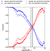 |
Fig. 7. Fractions of young (blue) and old (red) galaxies, as defined in Sect. 4.2, in 0.1 dex-wide mass bins. Filled and empty symbols refer to fractions derived from aperture-corrected estimates and uncorrected estimates, respectively. The solid and dashed vertical lines identify the transition masses based on the aperture corrected (Mtrac = 1010.80 M⊙) and uncorrected (Mtr = 1010.65 M⊙) estimates, respectively. |
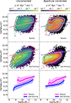 |
Fig. 8. Number density of passive (top row) and star-forming (middle row) galaxies in the mass-age plane, obtained using both the volume and completeness statistical corrections. Following the same colour-code of Fig. 3, we show the distributions obtained without the use of the aperture corrections (left panels) and the distributions obtained implementing aperture corrections (right panels). The contours identify the levels containing 16%, 50%, 84%, and 97.5% of the complete galaxy sample. The red and blue lines identify the divisions between young and old galaxies as defined in Sect. 4.2. The bottom panels display the median relations (solid lines) and the respective 16th and 84th percentiles (shaded area) as a function of mass, for passive (magenta) and star-forming (blue) galaxies. |
4.3. The scaling relations of star-forming and passive galaxies
Previous studies have shown that passive and star-forming galaxies obey different scaling relations (Mateus et al. 2006; González Delgado et al. 2015; Schawinski et al. 2014; Peng et al. 2015; Trussler et al. 2020; Looser et al. 2024). We study the scaling relations of SDSS DR7 galaxies separately for star-forming and passive, based on the aperture-corrected star formation rate estimates by Brinchmann et al. (2004)11, as available from the MPA-JHU catalogues. More specifically, we adopt a cut based on the deviation from the star-forming main sequence as determined in Gallazzi et al. (2021):
 (8)
(8)
This relation is characterised by a dispersion σ = 0.3. We classified galaxies as passive if they fall below the relation by more than 2σ and as star-forming otherwise.
Figures 8 and 9 present the comparison of the mass-age and mass-metallicity relations for passive (top panels) and starforming (central panels) galaxies, respectively. The bottom panels display the median (solid line) and 16th-84th percentile range (shaded area) of the relations for star-forming (blue) and passive (magenta) galaxies. The left panels display the uncorrected distributions and the right panels display the aperture-corrected ones. In both figures the black and green contours identify the isodensity levels. In Fig. 8 the blue and red lines identify the separations between young and old galaxies as defined in Sect. 4.2. From the mass-age plane we see that star-forming and passive galaxies follow different relations (as already observed by Schawinski et al. 2014; Peng et al. 2015; Trussler et al. 2020). As expected, star-forming and passive galaxies are mainly associated to the young and old sequences identified in Fig. 3, respectively. However, the mass-age distribution of passive galaxies presents a significant tail of young galaxies, which is visible at all masses below ∼1011 M⊙, and becomes particularly conspicuous below ∼109.5 M⊙, especially in the aperture-corrected version. These low-mass passive galaxies are indeed characterised by young stellar populations, with ages below the dividing line (∼109.4 yr), consistent with the ages of starforming galaxies of similar mass. On the other hand, high-mass star-forming galaxies reach light-weighted ages up to ∼109.6 yr, very similar to their passive counterparts. Star-forming galaxies reach higher ages in the low-mass end when aperture-corrections are taken into account, as already seen in the left panel of Fig. 3. Moreover, passive low-mass galaxies display both lower ages and a narrower distribution when aperture corrections are implemented.
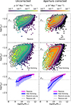 |
Fig. 9. Same as Fig. 8, but for the metallicity-mass distributions. The solid and dot-dashed black lines in the bottom panels identify the median MZRs obtained with the subsamples of passive-young and passive-old galaxies, respectively. The dotted horizontal lines indicate the solar metallicity of Z⊙ ≡ 0.02. |
The differences in the classifications according to sSFR (passive versus star-forming) or according to age (old versus young) are apparent when comparing their mass functions. In Fig. 10 we show the mass-functions of the galaxy sample (with aperture corrections implemented) obtained when separating galaxies based on the age (left panel) and on the star formation activity (right panel). Solid and dot-dashed lines represent the samples with S/N ≥ 10 and S/N ≥ 20, respectively, which, thanks to the statistical weights computed in Sect. 2.2, behave in a very consistent way. We find that the mass-functions of passive and old galaxies (red lines) have an overall similar shape, in accordance to a general correspondence between light-weighted ages and star formation activity. However, the mass-function of old galaxies is overall less populated and particularly suppressed at masses ≲1010.3 M⊙, reflecting the fact that the population of passive galaxies is characterised by light-weighted ages younger than the separation defined in Sect. 4.2, especially at the low-mass end. This, in turn, leads to lower transition mass between star-forming and passive galaxies (dot-dashed vertical lines in Fig. 10, Mtr ∼ 1010.3 M⊙) with respect to the transition mass between young and old galaxies (solid vertical lines in Fig. 10, Mtr = 1010.80 M⊙), corresponding to a difference of 0.5 dex, namely, a factor of ∼3.
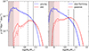 |
Fig. 10. Mass function of the S/N ≥ 10 (solid lines) and S/N ≥ 20 (dot-dashed lines) galaxy samples, including aperture corrections. Galaxies are divided into young (blue) and old (red), following the division described in Sect. 4.2(left panel) and divided into star-forming (blue) and passive (red), following the Gallazzi et al. (2021) separation, as per Eq. (8) (right panel ). The solid and dot-dashed black lines identify the transition masses obtained from the mass-functions, for the separations based on the age and SFR, respectively. The shaded areas identify the mass ranges where our sample is not representative, namely ≲M⋆ ∼ 109.5 M⊙ for passive/old galaxies (red shading), ≲M⋆ ∼ 109 M⊙ for star-forming and young galaxies (grey shading). Notably, the statistical weights ensure that we recover consistent mass functions irrespective of the S/N cut. |
From the MZRs of Fig. 9 we see that star-forming and passive galaxies follow distinct MZRs (as already observed by Peng et al. 2015; Trussler et al. 2020; Gallazzi et al. 2021; Looser et al. 2024). At any given M⋆ passive galaxies are located at higher median metallicities. Furthermore, when considering aperture-corrections, they follow a flatter and narrower relation with respect to star-forming galaxies. Although passive galaxies are located at higher median metallicities, they significantly overlap with the distribution of star-forming galaxies (bottom panels of Fig. 9), resulting in a broad yet unimodal MZR when the whole sample is considered (bottom panels of Fig. 3). Analysing the uncorrected MZRs for passive and star-forming galaxies we see that they have only a marginal separation, as opposed to the very clear difference observed in the aperture-corrected ones. Furthermore, not implementing aperture corrections affects also the slopes of both MZRs.
In Appendix B we show that the partial MZRs obtained by splitting the sample into young and old galaxies are in substantial agreement with the ones obtained based on the splitting on the SFR. However, looking at the MZRs of young passive galaxies (solid black line, in the bottom panels of Fig. 9), i.e. of those galaxies that have a discordant classification based on age and on SFR, we see that they follow essentially the same relation as the passive old ones (dotted black line, in the bottom panels of Fig. 9). This is indicative, somewhat surprisingly, of a stronger link of the stellar MZR with the current SFR (on 107 yr timescale), rather than with the mean age, which characterises the full extent of the SFH of a galaxy.
It is worth emphasizing again that aperture corrections are fundamental to correctly characterise the differences between the scaling relations of star-forming, passive, young, and old galaxies. In particular, in the mass-age relation the corrections significantly affect passive low-mass galaxies, which turn out to have very similar ages to equally massive star forming galaxies. Moreover, in the mass-metallicity plane they are critical in assessing whether passive and star-forming galaxies obey different MZRs, and correctly characterise their slopes. Such a differentiation has been used in several works to derive constraints on the mechanisms producing galaxy quenching (Peng et al. 2015; Trussler et al. 2020; Looser et al. 2024) and test chemical evolution models (e.g. Spitoni et al. 2017).
5. Assessment of the systematic biases and uncertainties
As already mentioned in previous sections, our new determinations of the mass-age and mass-metallicity scaling relations are based on SPS models with a number of improvements with respect to previous studies, in particular Gallazzi et al. (2005) and Gallazzi et al. (2021) (G05; G21, hereafter). In this section we analyse in detail the effect of the changes in the SPS modelling and parameter estimation. To do so we compare our results with the benchmark of (G05), which are the closest relations to ours in terms of the methodology for properties estimation. G05 employed the same Bayesian inference method used in this work (described in Sect. 3.1) to derive the full posterior PDF of the physical parameters of observed galaxies. However, their inference differs from ours in several aspects, including the dataset of observational constraints, the SPS models adopted to generate the prior CSP model library, and the treatment of dust attenuation.
G05 analysed the SDSS DR2 (Abazajian et al. 2004), which differs from the DR7 both for the more limited statistics, and for the data reduction pipeline, which directly affects the measurements of the absorption indices from the galaxies spectra. Considering the modelling, we introduced several changes to the SPS models, including updates to the stellar spectral library and 2D evolutionary tracks, more complex SFHs and CEHs prescriptions, and an explicit modelling of the dust content (see Table 1 for a summary of these changes, first and last rows for G05/G21 and this work, respectively). Another fundamental difference with respect to G05 resides in the method used to model and infer dust attenuation and its effect on the mass determination (see Sect. 5.2.1 for more details).
Ingredients of the SPS models used in the comparison for the assessment of the systematics.
Since in this section we want to isolate and characterise the importance of these changes for the scaling relations, we will consider estimates obtained without the implementation of aperture corrections, for consistency with previous works.
5.1. Cumulative effects of the changes in SPS modelling
The bottom panels (i, j) of Fig. 11 show the distributions in the mass-age and mass-metallicity planes for the SDSS DR7 sample studied in this work. Differently from Fig. 3, we show the distributions normalised in each bin of mass12. The black lines identify the median (solid) and 16th and 84th percentiles (dashed) of the galaxy distribution in bins of mass. Additionally we plot the median relations of G05 (red lines).
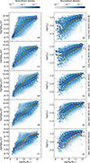 |
Fig. 11. Density of galaxies normalised in each mass bin (same as Fig. 8 from Gallazzi et al. 2005) for the mass-age (left) and mass-metallicity (right) relations obtained with each SPS model in Table 1 (one model in each row). In each panel the black solid and dashed lines identify the median and 16th and 84th percentiles of the corresponding distribution in mass bins, while the yellow line identifies the median relations in the respective plane taken from Gallazzi et al. (2021). The last row displays the distributions for the fiducial models of this work. In these panels, the red line represents the original G05 scaling relations. Note: these results are obtained without aperture corrections, for consistency with G05 and G21. The dotted horizontal lines in the mass-metallicity planes indicate the solar metallicity of Z⊙ ≡ 0.02. |
The bottom panels (i, j) of Fig. 11 illustrate the cumulative effects on the scaling relations due to the changes in the SPS modelling and to the observational dataset, going from G05 to the present work. To isolate the effect of the improvement in the data from SDSS DR2 to SDSS DR7 we also plot the G21 relations (yellow lines). The latter were obtained with the same SPS model and inference method of G05, but based on the SDSS DR7. The differences between the median relations of G05 and G21 are negligible at the high-mass end for both mass-age and mass-metallicity scaling relations. For M⋆ ≲ 1010 M⊙ G21 estimates higher median ages and metallicities in comparison to G05, for a given galaxy mass. For masses below ∼109.2 M⊙ G05 has flatter relations in both mass-age and mass-metallicity with respect to G21.
Nonetheless, comparing G21 results with our relation, we find significant differences, which cannot be due to anything else than the different modelling. We see that our mass-age relation is flatter over the whole mass range. Furthermore, for masses below ∼109.6 M⊙ we obtain significantly higher light-weighted ages, with differences up to ∼0.25 dex. For higher stellar masses, our median relation predicts lower light-weighted ages, with differences up to ∼0.2 dex. The differences obtained for masses in the range 1010 − 1011 M⊙ are connected to the bimodality analysed in Sect. 4.1. In the mass-metallicity plane our relation has a shape similar to the G21, but shifted by ∼0.25 dex towards higher metallicities. In summary, the bottom panels of Fig. 11 show that the changes in the modelling (Table 1, first and last rows), are the main reason for the changes in the scaling relations between this work and G05, while the improvement due to the different SDSS data releases has only a minor effect.
5.2. Relevance of the changes in the ingredients of SPS models
In this section, we analyse the impact of the changes introduced in the main ingredients of the SPS models. To achieve this, we analysed the scaling relations derived from SPS models that progressively transition, one ingredient at a time, from the G05 and G21 models to the one adopted in this work. The changes were introduced sequentially and presented in the order they were implemented in the models. Following our analysis of the effects of the improvement in the dataset, the following comparisons will be performed only with the G21 results. The different versions of the models, which we use in the comparisons, are listed in Table 1. We start by comparing the G21 results with the ones we obtain when introducing an explicit dust treatment in the SPS models (which directly impacts the colours, but not the dust insensitive indices) and a different inference for the dust absorption (Sect. 5.2.1). Next we show the effect of updating the stellar spectral library, on which the SPS spectra are based, from STELIB (Le Borgne et al. 2003) to MILES, which has a direct impact on indices strengths and colours at fixed isochrone (Sect. 5.2.2). Subsequently, we change the SFH (delayed Gaussian + bursts instead of a decaying exponential + bursts), allowing for a phase with a rising SFR (Sect. 5.2.3). In the next step we implement a time dependent CEH (instead of fixed metallicity), allowing for a monotonic rise of Z⋆ (Sect. 5.2.4). Finally, we consider the effect of updating the stellar evolutionary tracks (PARSEC instead of Padova94 Alongi et al. 1993; Bressan et al. 1993; Fagotto et al. 1994a,b; Girardi et al. 1996), which modifies the isochrones, hence impacting index strengths and colours, and the way they map age and metallicity (Sect. 5.2.5). Additionally, the new isoschrones come with an extension of the metallicity range to higher values.
Figure 11 presents the mass-age (left-hand panels) and mass-metallicity (right-hand panels) relations normalised in each bin of mass. Each row displays the relations obtained with a specific model version, identified by the label on the right side. In each panel the yellow line represents the median relation from G21, while the black lines identify the median (solid) and 16th and 84th percentiles (dashed) of the distribution obtained for the given model version.
5.2.1. Dust treatment
With respect to G05 and G21 we introduced changes in the dust treatment both in the SPS modelling and in the estimation method. CSP models in the prior distribution are created with a given dust content, whose attenuation is obtained with the two-component model of Charlot & Fall (2000). In our bayesian framework the photometry is used jointly with absorption indices to estimate the PDF of attenuation, as well as of the stellar populations parameters. G05 and G21, instead, employed dust-free models. They estimated the colour excess from the difference between the r − i colour of the galaxy and the r − i colour of the dust-free model. Then they estimated the z-band attenuation Az assuming a single power law (λ−0.7) attenuation curve (Charlot & Fall 2000)13.
To analyse the effect of this difference for the dust treatment we compare the G21 with the Exp_FixZ_BC03_STELIB model version, which differs from the G05 and G21 only for the dust treatment. We find notable differences both in the mass-age (Fig. 11, panel a) and mass-metallicity (Fig. 11, panel b) planes. In the mass-age plane, for stellar masses below 1010 M⊙, the Exp_FixZ_BC03_STELIB version produces higher estimates for the light-weighed ages, with differences up to ∼0.3 dex. For higher masses, the G21 estimates higher ages with maximum difference of ∼0.15 dex at M⋆ ∼ 1011 M⊙. With increasing galaxy mass the differences get smaller, becoming negligible at the high-mass end. In the mass-metallicity plane the Exp_FixZ_BC03_STELIB version predicts higher stellar metallicities with respect to G21, with differences up to ∼0.2 dex in the low-mass end. The two relations have similar shapes, but the Exp_FixZ_BC03_STELIB predicts a relation that is flatter at the low-mass end and steeper at the high-mass end. All in all, the different dust treatment and the inclusion of photometry as an actual constraints affect the age and metallicity estimates in a mass-dependent way.
5.2.2. Stellar spectral Libraries
To assess the impact of the adopted stellar spectral libraries, we compare the outcomes of the inferences of the Exp_FixZ_BC03_STELIB model, which is based on BC03 SSPs built on the STELIB stellar library (Le Borgne et al. 2003), with the results of the Exp_FixZ_BC03_MILES model, based on the BC03 SSPs built on the MILES stellar library (Sánchez-Blázquez et al. 2006)14.
Before analysing the scaling relations, it is worth considering how the two sets of SSP tracks used to generate the CSP model libraries (dubbed ‘BC03_STELIB’ and ‘BC03_MILES’, respectively) differ in the index-index planes. Figure 12 displays different SSP tracks in the HδA+HγA versus D4000n and HδA+HγA versus [MgFe]′ indices planes. The BC03_STELIB and BC03_MILES SSP tracks are represented by the solid and dotted lines, respectively. The left, central, and right panels are associated to metallicities of Z⋆ = 0.004, Z⋆ = 0.02, and Z⋆ = 0.05 respectively. The colour code along the SSP tracks identifies the age of the stellar population; furthermore cyan, yellow, and red symbols identify ages of 109 yr, 109.5 yr, and 1010 yr, squares for BC03_STELIB and circles for BC03_MILES.
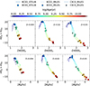 |
Fig. 12. Evolutionary tracks in the HδA+HγA vs. D4000n and HδA+HγA vs. [MgFe]′ index planes for the BC03_STELIB (solid), BC03_MILES (dotted), and CB19_MILES (dashed) SSPs (see Table 1 for more details). Left, central and right panels are associated to SSPs with different stellar metallicities: sub-solar (Z⋆ = 0.004), approximately solar (Z⋆ = 0.02), and super-solar (Z⋆ = 0.05 for BC03_STELIB and BC03_MILES, Z⋆ = 0.05 fro CB19_MILES) respectively. The tracks are colour-coded by the age of the SSP, and the points plotted onto the tracks identify ages of 108.5 yr, 109 yr, 109.5 yr, and 1010 yr, corresponding to different SSP models, squares for BC03_STELIB, circles for BC03_MILES, and stars for CB19_MILES. |
The BC03_STELIB and the BC03_MILES SSP tracks display significant differences especially at the lowest metallicities. Furthermore, there are significant age offsets even when the tracks overlap. Looking at the symbols as a reference, it is apparent that, at fixed index values, the BC03_MILES SSPs predict lower ages with respect to the BC03_STELIB ones, with stronger differences for older stellar populations. Where the tracks do not overlap, for a given value of HδA+HγA, the BC03_MILES is often located at lower values of [MgFe]′, which are associated to more metal poor stellar populations. Therefore, for a given observed value of the absorption indices, we expect BC03_MILES model to deliver younger ages and higher metallicities than BC03_STELIB.
The scaling relations normalised in mass bins obtained with the models implementing the STELIB and MILES stellar libraries show noticeable differences both in the mass-age (Fig. 11, panel c) and mass-metallicity (Fig. 11, panel d) planes. The SP parameters obtained with the Exp_FixZ_BC03_MILES model library display a systematic reduction in stellar age estimates for masses above ∼109.5 M⊙, with respect to Exp_FixZ_BC03_STELIB. In the mass-metallicity plane we find an increase of the metallicity for masses M⋆ ≲ 1010 M⊙, with differences up to ∼0.25 dex. While systematic differences in SSPs are not trivially transposed to CSPs and, in turn, to SP parameter estimates, the most significant differences in the scaling relations mirror the most outstanding differences in the SSPs. The largest age differences are found for stellar populations older than ∼109.3 yr, while the largest metallicity differences affect metal poor populations at thelow-mass end.
5.2.3. Star formation history
Another substantial change we introduced in this work, with respect to G21, concerns the SHF. Both the SFHs used in this work and in G21 are composed by a continuous component superimposed with random bursts of star formation to simulate stochasticity and rejuvenation phenomena. G21 adopts a decaying exponential SFR(t)∝exp(−γt) as continuous component, characterised by two parameters: tform identifying the look-back time at which the SFH starts, and γ, the characteristic e-folding time. In this work, the continuous component is modelled with a delayed Gaussian function (Sandage 1986; Gavazzi et al. 2002, see Eq. 5, Sect. 3.2). In addition to purely declining SFHs, this formalism allows for a phase of increasing SFR, whose extent is parametrised by the characteristic timescale τ in relation to the formation time tform. This results in more flexibility and a more extended coverage of the stellar population parameter space.
With the implementation of a new SFH we also extended the maximum tform, lb, reaching values up to 20 Gyr look-back time. This extension above the cosmologically motivated 14 Gyr limit has been introduced to avoid skewing the age posterior of very old galaxies, which would have a hard boundary at the maximum tform, lb for the old tail and practically no limitation for the young tail.
Using the Exp_FixZ_BC03_MILES as a starting point, we replaced the exponential continuous component with the Sandage, while keeping all other ingredients fixed, and created a new model library called San_FixZ_BC03_MILES. With the stellar population parameters inferred with this new library, we analysed the systematic effect of the SFH relative to Exp_FixZ_BC03_MILES. In the scaling relations, the implementation of this new SFH has significant effects regarding the age estimates and little importance for stellar metallicity estimates (shown in panels e and f of Fig. 11). The new age estimates result in lower light-weighted ages for masses between ∼109.2 M⊙ and ∼1011 M⊙. For M⋆ ≳ 1010.5 M⊙ the median relation steepens, reaching the same median light-weighted ages of the Exp_FixZ_BC03_MILES model in the high-mass end. We also see that massive old galaxies have a broader age distribution, reaching higher light-weighted ages when compared to the estimates obtained with the previous implementation of the SFH. We argue that these difference could be due, at least partly, to the removal of the prior-induced bias, thanks to the extension of the maximum tform, lb up to 20 Gyr. This mass-dependent changes in the slope of the median relation is connected to the formation of a bimodal mass-age distribution, characterised by two separate sequences of young and old galaxies with a transition in the mass range 1010 − 1011 M⊙. The change in the SFH impacts only weakly the MZR, causing a shift of ≲0.1 dex towards higher metallicities for masses above 1010 M⊙.
5.2.4. Chemical enrichment history
The reference CSP library adopted in this work implements a parametric CEH (see Eq. 6, Sect. 3.2), which incorporates a dependence on the formed stellar mass, thereby establishing a connection with the SFH. As opposed, G21 assumes a constant metallicity along the SFH, randomly drawn from a logarithmic distribution in the range 0.2 − 2.5 Z⊙. To assess the systematics induced by the implementation of this different CEH, we compare the outcome of the inference obtained with the San_FixZ_BC03_MILES model and the model implementing the new parametric CEH, which will be called San_VarZ_BC03_MILES and correspond to the libraries adopted in Zibetti et al. (2017, 2020), Zibetti & Gallazzi (2022).
The implementation of the variable CEH has significant effects both in the age and metallicity estimates (as shown in panels g and h of Fig. 11). In the mass-age plane we observe a strong increase of light-weighted ages of massive galaxies with old stellar populations. This results in the shift of the old sequence around Agewr ≳ 109.9 yr at stellar masses above 1010.5 M⊙. On the other hand the galaxies populating the young sequence do not change significantly their age estimates. These changes altogether enhance the bimodality in the mass-age distribution. In the mass-metallicity plane, we detect an increase in stellar metallicity for M⋆ ≤ 1011 M⊙ with increasing differences up to ∼0.1 dex with decreasing galaxy mass. Consequently, these variations in metallicity estimates lead to a flattening of the MZR at lower masses.
The increase in light-weighted stellar metallicities can be understood considering the different contribution to the absorption lines of stars of different ages and the fact that the assumed CEH imposes older stars to be metal poorer. With respect to a model with fixed metallicity, Z⋆, a model with variable metallicity having the same mean light-weighted metallicity, Z⋆, would produce weaker absorption lines, as the cooler stars responsible for the strongest absorption are bound to be at lower metallicity than the hotter stars. Reversely, at given index strength, a model with variable metallicity would need higher mean light-weighted metallicity than a fixed-metallicity model to reproduce the absorptions. The changes in age estimates can be seen as a side effect of the metallicity estimates caused by the classic age-metallicity degeneracy as well as by the CEH being linked to the SFH.
5.2.5. Evolutionary tracks
The latest version (CB19) of the Bruzual & Charlot (2003) SSP models implements the new PARSEC (Bressan et al. 2012; Marigo et al. 2013; Chen et al. 2015) stellar evolutionary tracks. The CB19 SSPs extend the maximum metallicity, reaching up to Z⋆ = 0.06, compared to the BC03, which are limited to Z⋆ = 0.05. We note that the PARSEC evolutionary tracks have a maximum age of 14 Gyr, as opposed to 20 Gyr for the Padova94 tracks. In order for the SFHs to maintain the maximum tform, lb to extend to 20 Gyr (see previous section), we slightly modify the synthesis of the CSPs by moving the weights of all components with age larger than 14 Gyr to the 14 Gyr component. To assess the impact of the implementation of these updated evolutionary tracks we compare the outcome of the inference obtained with the Padova94-based San_VarZ_BC03_MILES model library with the new San_VarZ_CB19_MILES PARSEC-based library.
Before analysing the differences in the scaling relations, we compared the different SSPs in the indices planes shown in Fig. 12. The BC03_MILES and CB19_MILES SSPs are identified in the figure by the dotted and dashed lines, respectively. We note that in the right panels the comparison for the SSPs at super-solar metallicity is not exact, as the same metallicity is not available for both SSPs. Therefore, we chose to show the comparison for the closest pair of super-solar metallicity, namely Z⋆ = 0.05 for BC03_MILES, and Z⋆ = 0.04 for CB19_MILES.
The two SSP models are in substantial agreement in terms of coverage of the index planes for Z⋆ ≲ Z⊙, while somewhat larger discrepancies appear at super-solar metallicity (note however the non-perfect match). Looking at the symbols, it is notable that for stellar populations younger than ∼109 yr, for a given combination of index values the CB19_MILES SSPs imply higher ages by ∼0.2 dex with respect to the BC03_MILES. For older stellar populations we observe negligible age differences (≲0.1 dex). At Z⋆ ≳ Z⊙ the tracks are offset with respect to each other, so in this regime we can expect systematic effects both in age and in metallicity.
To assess the systematics due to the change of the evolutionary tracks we analyse the mass-age and mass-metallicity relations obtained with the San_VarZ_CB19_MILES model (shown in panels i and j of Fig. 11). The most significant effects in the mass-age relation are mostly at the high-mass end, causing a shift of ∼0.15 dex towards lower light-weighted ages for old (Agewr ≳ 109.75 yr) and massive galaxies (M⋆ > 1011 M⊙)15. In the MZR the effects are generally negligible, except for a slight general increase in metallicity of the order of a few 0.01 dex and a similar reduction of the scatter at the high-mass end.
5.3. Goodness of fits for different CSP model libraries
We analyse the χ2 distribution for the fit performed with the Exp_FixZ_BC03_STELIB and San_VarZ_CB19_MILES models to analyse if the model changes introduced in this work allow us to fit the data more accurately. In Fig. 13 we show the maps of the median value of χmin2 (i.e. the χ2 of the best fitting model in a maximum likelihood sense), for the Exp_FixZ_BC03_STELIB (left panels) and the San_VarZ_CB19_MILES (right panels) model versions, in the mass-age plane (top row) and mass-metallicity plane (bottom row)
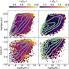 |
Fig. 13. Mass-age and mass metallicity distributions colour-coded by the median value of the χmin2 for estimates based on the Exp_FixZ_BC03_STELIB model library (same as in G05 and G21, left panels) and the SanCB19_MILES model library (reference models in this work, right panels). See Table 1 for more details about the SPS models. The black and green lines identify the density levels enclosing 16%, 50%, 84%, and 97.5% of the complete galaxy sample. The dotted horizontal lines in the mass-metallicity planes indicate the solar metallicity of Z⊙ ≡ 0.02. |
The contours identify the isodensity levels of the galaxy sample (S/N ≥ 10 and S/N ≥ 20 for age and metallicity, respectively). We see that the Exp_FixZ_BC03_STELIB model produces best fits with ⟨χmin2⟩∼4 for the majority of galaxies, without any correlation with the physical parameters of the galaxies. When implementing the model changes analysed in previous sections, we observe a reduction of the χmin2, obtaining ⟨χmin2⟩∼2. We also note that both models show an increase of the χmin2 for galaxies near the edges of the distributions, especially in the mass-metallicity plane. However, the San_VarZ_CB19_MILES models outperform the old models in terms of quality of the fit especially near the edge of the distribution, by significantly lowering the typical χmin2 from ∼10 to ∼5 at the high-metallicity end.
In conclusion, the new CSP model library adopted in this work result in an overall improved fit to the data. It is worth noting that, considering nine degrees of freedom (5 from absorption indices plus 5 from photometric bands minus 1 to allow for the normalisation) the obtained χmin2 values correspond to reduced χ2 well below 1. This indicates that our models actually overfit the data. Therefore, the uncertainties in the derived physical parameters are not driven mainly by observational errors data, rather they mostly stem from intrinsic degeneracies among the observed galaxy properties and the wide variety of CSPs that are able to reliably fit the data.
6. Discussion
In this work, we estimated stellar masses and mean light-weighted (and mass-weighted) ages for a sample of 354 977 SDSS DR7 galaxies in the Local Universe characterised by a spectroscopic S/N ≥ 10. For a subsample of 89 852 galaxies characterised by spectroscopic S/N ≥ 20, we also estimated the mean light-weighted (and mass-weighted) stellar metallicities. We performed a careful statistical characterisation of the samples, which has allowed us to compute the statistical weights to account for selection and incompleteness biases and obtain a volume-complete representation of the galaxy population. For the first time, we have implemented corrections to the spectroscopic properties of galaxies in order to mitigate the long-standing problem of SDSS fibre-aperture biases. Finally, in order to improve the accuracy in the stellar population parameter estimates, we employed more refined prescriptions for the CSP model libraries and adopted updated/state-of-the-art SSP models.
Based on this stellar population analysis, we have been able to characterise the distributions of Local Universe galaxies in the parameter space defined by stellar mass, age and metallicity, and made a preliminary exploration on their dependence on current SFR. In this section we discuss our results in the context of our current knowledge of galaxy evolution.
6.1. Importance of changes in SPS models
Comparing the scaling relations derived using different SPS models we analysed the systematic in the scaling relations effects induced by variations in individual model ingredients (see Sect. 5 and Fig. 11).
We found that the most significant changes in the mass-age relation arise from variations in the SFH, CEH, and evolutionary tracks. The adoption of a more refined SFH, which allows for a rising SFR and results in a better coverage of the observable space (i.e. the index-index space), has the strongest effect. Most notably, these changes lead to an enhancement of the mass-age bimodality, due to the presence of young galaxies for masses up to ∼1011 M⊙, which, in turn, determines a coexistence of the young and old sequences in the mass range 1010 − 1011 M⊙.
The updates in the evolutionary tracks and the implementation of a CEH caused significant changes in the mass-age distribution. The estimates obtained with the new CEHprescriptions result in a further enhancement of the age bimodality. On the other hand, with the updated PARSEC evolutionary tracks, we infer smaller ages for massive and old galaxies. Both effects have potentially strong implications in terms of galaxy evolution, especially concerning the quenching mechanisms (connected to the age bimodality) and the evolutionary time scales of the most massive galaxies. In the mass-metallicity plane, we found that the different ingredients implemented in the models have a significant impact and are strongly interlaced in affecting the MZR. The combination of all these updates in the model ingredients results in a shift of the relation towards higher metallicities, which is highly relevant for our understanding of galaxy chemicalenrichment.
6.2. Importance of aperture effects corrections
The SDSS spectroscopic data were obtained through 3″-diameter optical fibres centred on the centre of the target galaxies, extracting spectra from a (more or less, depending on the galaxy projected size) extended inner region. Since galaxies exhibit radial gradients in their stellar population properties, with a prevalence of older and more metal-rich stars in the centre and younger and more metal-poor stars in the outskirts (Pérez et al. 2013; Sánchez-Blázquez et al. 2014; González Delgado et al. 2014, 2015; Zibetti et al. 2017, 2020; Martín-Navarro et al. 2018; Goddard et al. 2017; Li et al. 2018; Johnston et al. 2022), this selective sampling may result in a bias in the measurement of spectral properties. This is a well-known observational bias, which is generally known as ‘aperture effects’ (Kauffmann et al. 2003a; Brinchmann et al. 2004; Gallazzi et al. 2005, 2008; Peng et al. 2015; Trussler et al. 2020). To correct this bias, in this work for the first time we implemented the corrections on the observed absorption indices calculated by Zibetti et al. (2025), which were derived using IFS CALIFA observations.
The resulting reduction of both light-weighted stellar ages and metallicities (Fig. 4) is qualitatively consistent with the expectations from a predominance of negative gradients in stellar ages and metallicities. Quantitatively we found that the strength of the aperture corrections varies with galaxy mass, becoming more significant at lower masses (Fig. 4). This mass-dependency stems from a mixture of different causes. On the one hand, the gradients are mass-dependent; on the other hand, they are linked also to galaxy morphology (which shows a connection with mass, see e.g. Nair & Abraham 2010). Furthermore the amplitude of the aperture corrections depends on the relative coverage of the SDSS spectroscopic fibres which, in turn, is determined by the galaxy apparent size (see Zibetti et al. 2025). Since more massive galaxies are typically observed at greater distances, their higher fibre coverage fraction compared to closer low-mass galaxies may further contribute to this effect. In addition, we observe an inverse effect in the mass-age plane for extremely young and low-mass galaxies, which increase both their light-weighted ages and stellar masses. This is in agreement with gradients observed by Pérez et al. (2013) and Johnston et al. (2022), which revealed that lower mass galaxies can experience an outside-in growth, with younger population located in the central part of the galaxy.
Comparing the galaxy properties estimates obtained with and without the implementation of aperture corrections we find qualitatively similar scaling relations, with a bimodal mass-age relation and a unimodal MZR of increasing age and metallicity estimates with increasing galaxy mass. However, when accounting for the aperture bias, we observe significant quantitative changes both in the populations of the sequences of the mass-age plane (top panels of Fig. 3), and in the slope of the MZR (bottom panels of Fig. 3). As we will discuss in more details in the next sections, the changes due to the implementation of the aperture corrections impact theoretical models of galaxy evolution and chemical enrichment. In particular, the enhancement of the population of galaxies in the young sequence may suggest that the efficiency of feedback processes may be less than what implied by previous stellar population analyses.
6.3. Constraints of galaxy quenching from the age bimodality
The distribution of galaxies in the mass-age plane is composed by two separate sequences of galaxies characterised by young (Agewr ≲ 109.3 yr) and old (Agewr ∼ 109.8 yr) stellar populations, as already shown in the Local Universe (e.g. Gallazzi et al. 2005; Peng et al. 2015; Sánchez et al. 2018; Trussler et al. 2020; Sánchez 2020). The former span the mass range from the lower completeness limit (∼109 M⊙) to 1011 M⊙, while the latter extends up to 1012 M⊙. These two sequences coexist and have similar population in the mass range 1010 − 1011 M⊙, defining a strongly bimodal age distribution. This bimodality is reminiscent of and connected to well-known bimodalities already observed in other galaxy properties, such as colour (e.g. Kauffmann et al. 2003b; Baldry et al. 2004; Schawinski et al. 2007, 2014), and SFR (e.g. Renzini & Peng 2015).
Our results support the idea of two distinct quenching pathways that depend on galaxy mass. On the one hand, the predominance of old stellar populations at the high-mass end indicates the presence of a mass-dependent mechanism responsible for galaxy quenching at high masses and at high redshift. The existence of a mass threshold beyond which galaxies evolve passively has been both pointed out observationally (Kauffmann et al. 2003b; Gallazzi et al. 2005; Moustakas et al. 2013; Haines et al. 2017) and derived theoretically (Dekel & Birnboim 2006; Cattaneo et al. 2006; Peng et al. 2010). This threshold is typically associated to the onset of processes that reduce or halt the inflow of gas from the IGM, ultimately shutting down star formation. These mechanisms include inefficient accretion due to shock heating in massive halos (Dekel & Birnboim 2006; Cattaneo et al. 2006) and black hole feedback, which can either deplete the gas reservoir through AGN-driven winds, or prevent further accretion from the IGM (Di Matteo et al. 2005; Croton et al. 2006; Schawinski et al. 2007; Fabian 2012; Cicone et al. 2014; Trussler et al. 2020; Bluck et al. 2020a,b). Nevertheless, the presence of a transition mass could also relate to other mechanisms capable of inducing quenching of star formation, even with the presence of a significant fraction of the molecular gas. An example of such a mechanism is ‘morphological quenching’ (e.g. Martig et al. 2009), by which the morphological transformation of a galaxy can stabilise the disk against gas cloud fragmentation. Moreover, resolved studies of star formation in Local Universe galaxies have shown that quenching is not a global process, but happens differently on several spatial scales (see review by Sánchez 2020 and references therein, also Zibetti & Gallazzi 2022). Recent studies based on SFRs and molecular gas fractions (fmol) have shown that quenching may originate from a suppressed star formation efficiency (SFE) in combination with a reduction in fmol (Saintonge et al. 2016, 2017; Colombo et al. 2020; Pan et al. 2024; Barrera-Ballesteros et al. 2025).
On the other hand, the coexistence of the young and old sequences in the mass-age plane at intermediate masses suggests that mass alone does not govern galaxy evolution. This aligns with several studies in the Local Universe, which have shown that passive low-mass galaxies are predominantly satellites that experienced quenching due to environmental processes such as starvation, ram-pressure stripping, and galaxy mergers (Larson et al. 1980; Balogh et al. 2000; van den Bosch et al. 2008; Pasquali et al. 2010; Schawinski et al. 2014; Gallazzi et al. 2021).
Both theoretical and observational studies place this transition between star-forming and passive galaxies at stellar masses of ∼1010.5 M⊙ ∼ 3 ⋅ 1010 M⊙ in the Local Universe. In this work we obtain an estimate of the transition mass between young and old galaxies of Mtr = 1010.65 M⊙ (neglecting aperture-corrections), which is 0.15 dex (a factor of ∼1.5) higher than previous Local Universe estimates. When accounting for the aperture bias the age estimates decrease for most of the galaxies in the sample. As a result the transition mass further increases, reaching Mtr = 1010.80 M⊙ ∼ 6 ⋅ 1010 M⊙ (Fig. 7). This upward shift in the transition mass serves as a crucial observational constraint for accurately modelling mass-driven galaxy quenching in theoretical frameworks of galaxy formation and evolution (e.g. Kauffmann 1996; De Lucia et al. 2006; Peng et al. 2010; Schaye et al. 2015; Pillepich et al. 2018). The fact that our aperture-corrected relations yield a higher transition mass than estimated in the past suggests that theoretical models of galaxy evolution should incorporate weaker quenching, possibly by reducing the efficiency of AGN feedback.
Our analysis of the young and old galaxy sequences shows that the old sequence is already populated at masses as low as M⋆ ∼ 109.5 M⊙, with approximately 10% of all the galaxies in this mass range lying above the separation (Figs. 3 and 7). Since most of the passive galaxies at these low masses are indeed satellites (Larson et al. 1980; Balogh et al. 2000; van den Bosch et al. 2008; Pasquali et al. 2010; Schawinski et al. 2014; Gallazzi et al. 2021), this result implies that, if environmental quenching is responsible for moving low-mass galaxies onto the old sequence, it must affect only a small fraction of the sample (less than 20% for M⋆ < 1010 M⊙). Conversely, if environmental quenching influences a significant fraction of the galaxy sample, it must have happened recently to avoid the transition of low-mass galaxies from the young to the old sequence. This has been further investigated by analysing the mass-age relation separating passive and star-forming galaxies (Fig. 8). The presence of a tail of passive low-mass galaxies with relatively young ages of ∼109.4 yr ∼ 2.5 Gyr suggests that the majority of low-mass passive galaxies have experienced environment quenching in the recent past; therefore, they can still populate the young sequence.
6.4. Correspondence between light-weighted ages and SFR estimates
To further investigate the SFH and possible quenching paths we analysed the mass-age relations dividing the galaxy sample between star-forming and passive using the measure of the sSFR, adopting the same selection criteria of Gallazzi et al. (2021). We showed that the majority of star-forming and passive galaxies populate the young and old sequences respectively (Fig. 8). Therefore, sSFR measures and light-weighted age estimates, although probing very different timescales (∼107 yr and ∼1 Gyr respectively), show a good correspondence for the majority of the galaxy sample. In accordance with similar analyses by Peng et al. (2015) and Trussler et al. (2020), this can be interpreted as evidence of galaxy quenching happening on timescales significantly longer than 1 Gyr. Consistent results have also been found by Corcho-Caballero et al. (2023a,b), who used the plane of observable defined by Hα versus D4000. These works have shown that the Hα−D4000 plane can be used to investigate how star-forming galaxies evolve into passive systems. They found that galaxies with high Hα equivalent widths (i.e. star-forming) generally have low D4000 (young stellar populations), while passive galaxies are generally characterised by high D4000 (old stellar populations). This general agreement between Hα equivalent widths and D4000 is interpreted as evidence of galaxies quenching through the so called ageing process (see also, Casado et al. 2015), which refers to a gradual decrease of the star formation activity on timescales longer than 1 Gyr.
Despite the general agreement between SFR estimates and light-weighted ages, we also find notable exceptions. On the one hand, star-forming galaxies display a tail of high mass galaxies characterised primarily by old stellar populations. We speculate that these may be green-valley galaxies, which display intermediate properties between star-forming and passive systems (Schawinski et al. 2014; Trussler et al. 2020). As they undergo the transition toward quenching, they may still retain some residual star formation activity. Alternatively, some of these galaxies could be passive systems that have recently undergone rejuvenation, making them detectable as star-forming, though without significantly altering their light-weighted ages. On the other hand we find a tail of passive galaxies with relatively young stellar populations (ages of ∼109.4 yr)16. We suggest that these may be recently quenched galaxies, in accordance with the analysis of the ageing diagram by Corcho-Caballero et al. (2023a,b)17.
To investigate the nature of galaxy quenching we carried out a detailed analysis of the fraction of galaxies in each of the four categories defined based both on star formation activity and light-weighted ages. In Fig. 14 we show the fraction of galaxies, obtained from the aperture corrected estimates, in each of the four categories: star-forming-old (black), star-forming-young (blue), passive-old (red), and passive-young (green). We confirm that passive-young galaxies constitute a significant fraction of the passive sample at low masses. In the low-mass end the fraction of passive-young galaxies is of ∼20% of the total sample and remains more or less constant with increasing galaxy mass, while the fraction of passive-old galaxies gradually increases. For masses above the transition mass the fraction of passive-young galaxies decreases, becoming negligible at M⋆ ∼ 1011.5 M⊙.
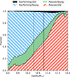 |
Fig. 14. Fraction of galaxies in the four categories of age and SFR classification, based on the aperture-corrected physical parameter estimates: star-forming-old (black), star-forming-young (hatched blue), passive-old (hatched red), and passive-young (green). The vertical dot-dashed line identifies the transition mass between star-forming and passive galaxies, obtained from the mass-functions in the right panel of Fig. 10. The vertical solid line identifies the transition mass between young and old galaxies, obtained as described in Sect. 4.2. |
The decrease of the fraction of passive-young galaxies above Mtr is connected to a more rapid increase of the passive-old fraction. This trend with M⋆ further supports the hypothesis of a change in the dominant quenching mechanism above the transition mass. In particular, the reduced fraction of passive-young galaxies indicates that the epoch of quenching is earlier or the timescale is shorter, or both. In addition the probability of rejuvenation might be reduced. We can interpret this as a manifestation of the mass quenching. For masses M⋆ ≥ Mtr, the mass-dependent quenching becomes dominant already at z ∼ 1 (Dekel & Birnboim 2006; Cattaneo et al. 2006; Peng et al. 2010), causing massive galaxies to evolve essentially passively. As a result, this causes the steep increase in light-weighted ages for passive galaxies across the transition mass (see Fig. 8). Below Mtr, environmental quenching becomes more dominant (Larson et al. 1980; Balogh et al. 2000; van den Bosch et al. 2008; Peng et al. 2010; Pasquali et al. 2010; Schawinski et al. 2014; Gallazzi et al. 2021). It may either have happened recently, resulting in lower light-weighted ages, or could have happened at higher redshift, resulting in low-mass old and passive galaxies.
To further investigate galaxy quenching, in a follow-up paper we build on this work focussing on constraining timescales for galaxies SFHs, providing deeper insights into the physical processes that regulate galaxy evolution.
6.5. Chemical evolution constraints from the MZR
The mass-metallicity plane displays a clear unimodal relation between galaxy mass and stellar metallicity, with a trend of increasing mean stellar metallicity with increasing galaxy mass (Fig. 3), in agreement with previous works in the local Universe (e.g. Gallazzi et al. 2005, 2021; Panter et al. 2008; Pasquali et al. 2010; Peng et al. 2015; Trussler et al. 2020; Zibetti & Gallazzi 2022; Looser et al. 2024) and extending towards higher redshifts (Gallazzi et al. 2014; Cappellari 2023; Nersesian et al. 2024; Gallazzi et al. 2025a,b). At the low-mass end the relation is steep, but it becomes shallower as galaxy mass increases. With our updated SPS modelling we obtained a shift of ∼0.25 dex towards higher metallicities with respect to previous works from our group (e.g. Gallazzi et al. 2005, 2021). The implementation of corrections for the SDSS aperture effects resulted in a mass dependent decrease of stellar metallicities, with stronger effects for lower mass galaxies (Figs. 3 and 4).
The existence of a MZR has been interpreted as evidence of galaxy downsizing (Cowie et al. 1996; Gavazzi & Scodeggio 1996; Gallazzi et al. 2005; Panter et al. 2008; Somerville & Davé 2015), whereby higher mass galaxies have assembled at earlier cosmic epochs and more rapidly, resulting in more efficient star formation and chemical enrichment. Another explanation for the shape of the MZR, which does not exclude downsizing, involves the presence of outflows which, depending on the galaxy gravitational potential, may cause losses of enriched gas. In fact, observational studies of the gas MZR and supernova driven outflows in Local Universe galaxies have shown that supernovae can shape the MZR by expelling significant quantities of enriched gas (Tremonti et al. 2004; Chisholm et al. 2018). This observational evidence suggest that more massive galaxies, thanks to their deeper gravitational wells, are less affected from metal rich outflows, reaching higher metallicities (Spitoni et al. 2017; Barone et al. 2018, 2020; Vaughan et al. 2022). On the other hand, the low metallicity of gas and stellar content of low-mass galaxies may suggest that they are able to maintain a metal poor gas reservoir due to infall of low-metallicity gas from the IGM, despite the ability of supernova-driven outflows to expel the enriched gas from the galaxy. This is supported by the discovery of the dependence of the MZR on the star formation activity of the galaxy. In fact several studies (e.g. Ellison et al. 2008; Lara-López et al. 2010; Mannucci et al. 2010) showed that more star-forming galaxies are located at lower median gas-phase metallicities with respect to less star-forming ones, defining the so-called Fundamental Metallicity Relation (FMR). Therefore, the normalisation and shape of the MZR result from a combination of several physical processes: metal removal via outflows; the infall of metal-poor gas from the IGM, leading to dilution of the enriched gas within galaxies; metal retention due to the gravitational potential; cosmic enrichment efficiency (see review by Maiolino & Mannucci 2019, and references therein).
Our updated and aperture-corrected MZR, which exhibits significant differences in both normalisation and shape compared to previous Local Universe studies, provides crucial insights for accurately modelling galaxy evolution. On the one hand, the shift towards higher metallicities at the high-mass end suggests that massive galaxies are more efficient at enriching the ISM than inferred from previous estimates of the stellar MZR, potentially requiring less efficient AGN driven outflows. Conversely, the steeper slope observed at lower masses suggests that weaker chemical enrichment efficiencies are required in the low-mass regime (with significant implications on supernova-driven outflows) and/or enhanced metal-poor gas infall are required to dilute the galaxy gas reservoir.
6.6. Constraints on galaxy quenching from the mass metallicity relation
As detailed in Sect. 6.3, one of the possible explanation for galaxy quenching involves a reduction of gas accretion due to the combination of shock heating of the gas accreting onto the dark matter halo (Dekel & Birnboim 2006; Cattaneo et al. 2006), and black hole feedback (Di Matteo et al. 2005; Croton et al. 2006; Schawinski et al. 2007; Fabian 2012; Cicone et al. 2014; Trussler et al. 2020). Lower mass galaxies may quench via starvation (Larson et al. 1980; Balogh et al. 2000; van den Bosch et al. 2008), or loose their gas reservoir due to supernova-driven winds (e.g. Dalcanton 2007) and ram pressure stripping (Larson et al. 1980; Abadi et al. 1999). Alternatively, mergers may result in morphological transformation either by disrupting the galaxy gas reservoir (e.g. Schawinski et al. 2014), or stabilising the disk against fragmentation, resulting in a lower SFE even in the presence of a significant fraction of molecular gas (e.g. Martig et al. 2009).
While both mergers and ram pressure stripping are associated to gas removal processes, starvation acts stopping the accretion of fresh gas from the IGM. As pointed out by Peng et al. (2015), gas removal and starvation leave different signatures in the MZR. Analysing the MZR for passive and star-forming galaxies separately, they conclude that galaxy quenching is characterised mostly by a prolonged period of starvation. More recently Trussler et al. (2020) supported this scenario invoking also the need of outflows to correctly reproduce the observed MZR. On the contrary, Spitoni et al. (2017) retrieved the observed MZR by developing an analytical model implementing an exponential declining gas infall coupled with strong galactic winds, reproducing the effect of starvation.
When analysing the MZR for passive and star-forming galaxies separately, we found that star-forming and passive galaxies follow two distinct MZRs (Fig. 9). The two relations are separated at the low mass end by ∼0.3 dex, but get progressively closer and eventually merge for masses M⋆ > Mtr. Nonetheless, star-forming galaxies always exhibit lower median metallicities than passive galaxies of the same mass, in agreement with Peng et al. (2015) and Trussler et al. (2020) results. The higher stellar metallicities of low-mass passive galaxies, coupled with their relatively young ages of ∼3 Gyr, suggest that star formation has continued in a metal-enriched ISM for an extended period. From our MZR we also find that the scatter of the metallicity distribution for star-forming galaxies is always bigger than the one of passive galaxies of the same mass. This may indicate that star-forming galaxies have more stochastic metallicity evolution. Alternatively, recent results by Looser et al. (2024) suggest that the scatter may be due to the superposition of the MZR of galaxies with different sSFR. These authors, based on MANGA observations, found that galaxies are located on different MZRs based on their sSFR, defining the so-called stellar Fundamental Metallicity Relation (stellar-FMR). This stellar-FMR thus represent the analogous of the already observed gas-FMR (Ellison et al. 2008; Lara-López et al. 2010; Mannucci et al. 2010).
In our work we also found that the MZRs of passive-young and passive-old galaxies display negligible differences, in contrast with the starkly different MZR of the star-forming ones (Fig. 9). This shows that the chemical enrichment is more tightly connected to the current star-formation activity (timescale ∼107 yr), rather than with the long-term SFH (timescale ≳109 yr). A physical interpretation of this observation is not straightforward, as a direct causation appears unplausible considering that the stellar metallicity is a fossil record of the chemical enrichment over the entire evolutionary history of a galaxy. Apparently, no matter what is the timescale of the mechanism that leads to the suppression of the SFR (either starvation or abrupt/mass-driven quenching), the result of quenching is invariably an enhancement of the stellar metallicity. We will investigate this problem in further details by studying the MZR in finer bins of SFR in a forthcoming paper. Yet, one should keep in mind that observational uncertainties, particularly those related to the statistical nature of the aperture corrections and the limited size of the passive–young subsample, may result in a cross-contamination of the different subsamples by galaxies that are misclassified in terms of SFR or age, and could partly contribute to the observed trends.
7. Summary and conclusions
We analysed the galaxies in the SDSS DR7 using state-of-the-art SPS modelling to estimate the galaxy masses, light-weighted and mass-weighted ages, and stellar metallicities. We used statistical weights to account for biases induced by sample selections and implemented novel corrections for SDSS aperture effects. We summarise the main findings obtained through our analysis of the mass-age and mass-metallicity relations of our sample of galaxies as follows:
-
In the mass-age plane, we obtained a distribution composed by two distinct sequences of young and old galaxies at ages of ∼109.3 yr and ∼109.8 yr, respectively. Furthermore, such sequences show a coexistence in the mass range 1010 − 1011 M⊙, leading to the formation of a bimodal distribution (Fig. 3).
-
In the mass-metallicity plane, we obtained a clear correlation between galaxy stellar mass and stellar metallicity, as already found in several other works in the literature, where lower-mass galaxies are characterised by lower values of stellar metallicity (Fig. 3). Furthermore our metallicity estimations are shifted of ∼0.25 dex towards higher metallicities, when compared to previous studies from the Local Universe, such as Gallazzi et al. (2005, 2021), mainly due to our updated and refined state-of-the-art modelling for SPS (see bottom panels of Fig. 11).
-
The implementation of novel aperture corrections to SDSS observations causes a reduction in stellar mass, age, and metallicity for most galaxies in our sample. In the mass-age plane, this leads to an enhancement of the population of galaxies in the young sequence at the expenses of the old one. In the mass-metallicity, there is a mass dependent decrease of the metallicity, with stronger effects for lower-mass galaxies, resulting in a not-uniform steepening of the relation (Figs. 3 and 4).
-
We estimated a transition mass (across which the population changes from being dominated by young galaxies to being dominated by old galaxies) of Mtr = 1010.80 M⊙, which is 0.15 dex higher than the value we would infer without accounting for aperture biases (Fig. 7). These estimates are higher than the usually quoted 1010.5 M⊙ in the literature (e.g. Kauffmann et al. 2003b; Gallazzi et al. 2005; Peng et al. 2010; Haines et al. 2017; Gallazzi et al. 2021).
-
Analysing the mass-age scaling relation separately for passive and star-forming galaxies, we found that for the majority of the galaxy sample, star-forming and passive galaxies correspond to galaxies characterised by young and old stellar population, respectively (Fig. 8). When implementing aperture corrections, we observed the presence of a significant fraction of passive galaxies with young stellar populations, which may have significant implication for satellite quenching. Similarly in the mass-metallicity plane, we confirmed results obtained in prior Local Universe studies, which showed that star-forming galaxies have lower median metallicities, compared to passive ones (see Fig. 9). When implementing aperture corrections the separation of the two MZRs is enhanced.
-
By analysing each difference in the SPS ingredients, we showed that each change causes noticeable effects (see Sect. 5). The most relevant ones for the mass-age relation can be ascribed to the SFH and CEH prescriptions, along with the choice of evolutionary tracks. For the MZR, each model change acts differently, but with similar importance in the shaping of the MZR.
Our work highlights the importance of controlling for systematic effects when comparing analyses on stellar populations conducted with different methods and models. Our scaling relations will serve as a zero point for scaling relation studies at intermediate redshift (0.3 − 1), already ongoing (e.g. LEGA-C van der Wel et al. 2016) or forthcoming (e.g. WEAVE-StePS Iovino et al. 2023b and 4MOST-StePS Iovino et al. 2023a), while extending towards cosmic noon with VLT-MOONS (Cirasuolo et al. 2020) and JWST. As the best practice, evolutionary studies should be conducted with consistent models and methods. The stellar population scaling relations for the LEGA-C sample at z ∼ 0.7 have been already analysed in a fully consistent way with the same models and methodology as in this paper by Gallazzi et al. (2025a,b). We intend to extend the same approach to the forthcoming WEAVE-StePS and 4MOST-StePS and to the samples observed with VLT-MOONS in the next few years. Within this very same SPS analysis framework, we will also extend the present analysis of the aperture-corrected properties of SDSS galaxies to include more detailed information about their SFH and chemical enrichment patterns and gain more insight on their evolutionary paths.
Data availability
The table containing the observed and estimated properties of the duplicate-combined SDSS DR7 galaxies is available at the CDS via https://cdsarc.cds.unistra.fr/viz-bin/cat/J/A+A/703/A5
The catalogues are available at the following link: https://wwwmpa.mpa-garching.mpg.de/SDSS/DR7/raw_data.html
We rejected galaxies with invalid (negative) estimates for redshift and velocity dispersion uncertainties. We also rejected galaxies with the z_warning flag greater than zero.
We used the kcorrect.none.petro.z0.00.fits and kcorrect.none.petro.z0.10.fits catalogues, which may be found at https://sdss.physics.nyu.edu/vagc-dr7/vagc2/kcorrect/
We relaxed the selection on Petrosian half-light surface brightness μ50 ≤ 24.5 mag arcsec−2, as this requirement is automatically matched for the S/N requested by the stellar population analysis.
This was done following the recommendations in https://www.sdss3.org/dr9/tutorials/flags.php#clean
With this selection, we rejected 822 galaxies with S/N ≥ 10 and 121 galaxies with S/N ≥ 20.
Note: the velocity dispersion σ⋆ is not corrected for the aperture effects; hence, the aperture-corrected indices are compared with model indices at the σ⋆ as measured within the fibre. This is not expected to cause significant biases, because the dependence of indices on σ⋆ is weak and the aperture effects on σ⋆ are typically small.
The CB19 SSPs are available at this link: https://www.bruzual.org/CB19/
Noting that for the CB19 SSPs, the maximum available age is 14 Gyr, therefore we render the oldest part of the SFH by modifying the weight for the 14-Gyr old component (see Sect. 5.2.5).
Errors on these parameters are obtained from a Monte Carlo realisation in which the slope is varied following a normal distribution centred on the mean slope with σ corresponding to half of the difference between the maximum and the minimum of the slope.
Aperture-corrected star formation rate estimates have been estimated by Brinchmann et al. (2004) based on galaxy colours. Corrections for galaxies with low levels of star formations were calculated building upon Salim et al. (2007), as described by the MPA-JHU catalogues documentation at: https://wwwmpa.mpa-garching.mpg.de/SDSS/DR7/sfrs.html
This is done similarly to Fig. 8 of G05. Note, however, that the distribution in Fig. 8 of G05 shows the stack of the PDFs of the physical parameters, while in this work we show the distributions of the fiducial estimates of each galaxy as given by the PDF medians.
See section 2.4.3 of Gallazzi et al. (2005) for more details.
Noting that the BC03 MILES-based SSPs were produced with the 2016 version of the BC03 code, which still has negligible differences in terms of optical indices with respect to the original BC03 code.
Noting that because of the different age extension of the two SSP grids and the way we modified the SP synthesis (see above), the prior in light-weighted mean age of the two libraries does not match exactly, with a possible bias towards younger ages for CB19.
Noting that the low SFR estimate for passive and young galaxies could possibly stem from the underestimation of the aperture corrections for the SFR. However, this is unlikely to be the case for the majority of these galaxies as we checked that their distribution of SFR aperture corrections is similar to the one for star-forming galaxies. Moreover, we also found that the fraction of light in fiber for passive young galaxies is typically somewhat larger than for star-forming, thus making the aperture corrections for these galaxies possibly less important.
Noting, however, that in Corcho-Caballero et al. (2023a,b) they refer to quenching when the transition between active star formation and passive evolution happens on timescales shorter than 1 Gyr, and to ageing otherwise. In this work, we have not made such differentiation and we use quenching to refer to every process that stops star formation.
Acknowledgments
We thank the referee for useful comments which have improved the clarity of our manuscript. This paper and related research have been conducted during and with the support of the Italian national inter-university PhD programme in Space Science and Technology. S.Z. acknowledges support from the INAF-Minigrant-2023 “Enabling the study of galaxy evolution through unresolved stellar population analysis” 1.05.23.04.01. A.R.G. acknowledges support from the INAF-Minigrant-2022 “LEGA-C” 1.05.12.04.01. L.S.D. is supported by the “Prometeus” project PID2021-123313NA-I00 of MICIN/AEI/10.13039/501100011033/FEDER, UE.
References
- Abadi, M. G., Moore, B., & Bower, R. G. 1999, MNRAS, 308, 947 [Google Scholar]
- Abazajian, K., Adelman-McCarthy, J. K., Agüeros, M. A., et al. 2004, AJ, 128, 502 [NASA ADS] [CrossRef] [Google Scholar]
- Abazajian, K. N., Adelman-McCarthy, J. K., Agüeros, M. A., et al. 2009, ApJS, 182, 543 [Google Scholar]
- Alongi, M., Bertelli, G., Bressan, A., et al. 1993, A&ASS, 97, 851 [Google Scholar]
- Asari, N. V., Cid Fernandes, R., Stasińska, G., et al. 2007, MNRAS, 381, 263 [Google Scholar]
- Baldry, I. K., Glazebrook, K., Brinkmann, J., et al. 2004, ApJ, 600, 681 [Google Scholar]
- Balogh, M. L., Morris, S. L., Yee, H. K. C., Carlberg, R. G., & Ellingson, E. 1999, ApJ, 527, 54 [Google Scholar]
- Balogh, M. L., Navarro, J. F., & Morris, S. L. 2000, ApJ, 540, 113 [Google Scholar]
- Barone, T. M., D’Eugenio, F., Colless, M., et al. 2018, ApJ, 856, 64 [Google Scholar]
- Barone, T. M., D’Eugenio, F., Colless, M., & Scott, N. 2020, ApJ, 898, 62 [NASA ADS] [CrossRef] [Google Scholar]
- Barrera-Ballesteros, J. K., Cruz-González, I., Colombo, D., et al. 2025, ApJ, 978, 23 [Google Scholar]
- Blanton, M. R., & Roweis, S. 2007, AJ, 133, 734 [NASA ADS] [CrossRef] [Google Scholar]
- Blanton, M. R., Hogg, D. W., Bahcall, N. A., et al. 2003, ApJ, 592, 819 [Google Scholar]
- Blanton, M. R., Schlegel, D. J., Strauss, M. A., et al. 2005, AJ, 129, 2562 [NASA ADS] [CrossRef] [Google Scholar]
- Bluck, A. F. L., Maiolino, R., Piotrowska, J. M., et al. 2020a, MNRAS, 499, 230 [NASA ADS] [CrossRef] [Google Scholar]
- Bluck, A. F. L., Maiolino, R., Sánchez, S. F., et al. 2020b, MNRAS, 492, 96 [Google Scholar]
- Bressan, A., Fagotto, F., Bertelli, G., & Chiosi, C. 1993, A&AS, 100, 647 [NASA ADS] [Google Scholar]
- Bressan, A., Marigo, P., Girardi, L., et al. 2012, MNRAS, 427, 127 [NASA ADS] [CrossRef] [Google Scholar]
- Brinchmann, J., Charlot, S., White, S. D. M., et al. 2004, MNRAS, 351, 1151 [Google Scholar]
- Bruzual, A. G. 1983, ApJ, 273, 105 [CrossRef] [Google Scholar]
- Bruzual, G., & Charlot, S. 2003, MNRAS, 344, 1000 [NASA ADS] [CrossRef] [Google Scholar]
- Bundy, K., Bershady, M. A., Law, D. R., et al. 2014, ApJ, 798, 7 [NASA ADS] [CrossRef] [Google Scholar]
- Camps-Fariña, A., Sanchez, S. F., Lacerda, E. A. D., et al. 2021, MNRAS, 504, 3478 [CrossRef] [Google Scholar]
- Camps-Fariña, A., Sánchez, S. F., Mejía-Narváez, A., et al. 2022, ApJ, 933, 44 [CrossRef] [Google Scholar]
- Cappellari, M. 2023, MNRAS, 526, 3273 [NASA ADS] [CrossRef] [Google Scholar]
- Casado, J., Ascasibar, Y., Gavilán, M., et al. 2015, MNRAS, 451, 888 [NASA ADS] [CrossRef] [Google Scholar]
- Cattaneo, A., Dekel, A., Devriendt, J., Guiderdoni, B., & Blaizot, J. 2006, MNRAS, 370, 1651 [NASA ADS] [CrossRef] [Google Scholar]
- Chabrier, G. 2003, PASP, 115, 763 [Google Scholar]
- Charlot, S., & Fall, S. M. 2000, ApJ, 539, 718 [Google Scholar]
- Chen, Y., Bressan, A., Girardi, L., et al. 2015, MNRAS, 452, 1068 [Google Scholar]
- Chisholm, J., Tremonti, C., & Leitherer, C. 2018, MNRAS, 481, 1690 [NASA ADS] [CrossRef] [Google Scholar]
- Cicone, C., Maiolino, R., Sturm, E., et al. 2014, A&A, 562, A21 [NASA ADS] [CrossRef] [EDP Sciences] [Google Scholar]
- Cid Fernandes, R., Asari, N. V., Sodré, L., et al. 2007, MNRAS, 375, L16 [NASA ADS] [CrossRef] [Google Scholar]
- Cirasuolo, M., Fairley, A., Rees, P., et al. 2020, The Messenger, 180, 10 [NASA ADS] [Google Scholar]
- Colombo, D., Sanchez, S. F., Bolatto, A. D., et al. 2020, A&A, 644, A97 [EDP Sciences] [Google Scholar]
- Corcho-Caballero, P., Ascasibar, Y., Cortese, L., et al. 2023a, MNRAS, 524, 3692 [Google Scholar]
- Corcho-Caballero, P., Ascasibar, Y., Sánchez, S. F., & López-Sánchez, Á. R. 2023b, MNRAS, 520, 193 [NASA ADS] [CrossRef] [Google Scholar]
- Cowie, L. L., Songaila, A., Hu, E. M., & Cohen, J. G. 1996, AJ, 112, 839 [Google Scholar]
- Croton, D. J., Springel, V., White, S. D. M., et al. 2006, MNRAS, 365, 11 [Google Scholar]
- da Cunha, E., Charlot, S., & Elbaz, D. 2008, MNRAS, 388, 1595 [Google Scholar]
- Dalcanton, J. J. 2007, ApJ, 658, 941 [CrossRef] [Google Scholar]
- De Lucia, G., Springel, V., White, S. D. M., Croton, D., & Kauffmann, G. 2006, MNRAS, 366, 499 [NASA ADS] [CrossRef] [Google Scholar]
- Dekel, A., & Birnboim, Y. 2006, MNRAS, 368, 2 [NASA ADS] [CrossRef] [Google Scholar]
- Di Matteo, T., Springel, V., & Hernquist, L. 2005, Nature, 433, 604 [NASA ADS] [CrossRef] [Google Scholar]
- Ellison, S. L., Patton, D. R., Simard, L., & McConnachie, A. W. 2008, ApJ, 672, L107 [NASA ADS] [CrossRef] [Google Scholar]
- Erb, D. K. 2008, ApJ, 674, 151 [NASA ADS] [CrossRef] [Google Scholar]
- Fabian, A. C. 2012, ARA&A, 50, 455 [Google Scholar]
- Fagotto, F., Bressan, A., Bertelli, G., & Chiosi, C. 1994a, A&AS, 104, 365 [NASA ADS] [Google Scholar]
- Fagotto, F., Bressan, A., Bertelli, G., & Chiosi, C. 1994b, A&AS, 105, 29 [NASA ADS] [Google Scholar]
- Fontanot, F., De Lucia, G., Monaco, P., Somerville, R. S., & Santini, P. 2009, MNRAS, 397, 1776 [NASA ADS] [CrossRef] [Google Scholar]
- Fukugita, M., Ichikawa, T., Gunn, J. E., et al. 1996, AJ, 111, 1748 [Google Scholar]
- Gallazzi, A., Charlot, S., Brinchmann, J., White, S. D. M., & Tremonti, C. A. 2005, MNRAS, 362, 41 [Google Scholar]
- Gallazzi, A., Brinchmann, J., Charlot, S., & White, S. D. M. 2008, MNRAS, 383, 1439 [Google Scholar]
- Gallazzi, A., Bell, E. F., Zibetti, S., Brinchmann, J., & Kelson, D. D. 2014, ApJ, 788, 72 [Google Scholar]
- Gallazzi, A. R., Pasquali, A., Zibetti, S., & Barbera, F. L. 2021, MNRAS, 502, 4457 [NASA ADS] [CrossRef] [Google Scholar]
- Gallazzi, A., Zibetti, S., & van der Wel, A. 2025a, A&A, submitted [Google Scholar]
- Gallazzi, A., Zibetti, S., & van der Wel, A., 2025b, A&A, submitted [Google Scholar]
- Gavazzi, G., & Scodeggio, M. 1996, A&A, 312, L29 [NASA ADS] [Google Scholar]
- Gavazzi, G., Bonfanti, C., Sanvito, G., Boselli, A., & Scodeggio, M. 2002, ApJ, 576, 135 [NASA ADS] [CrossRef] [Google Scholar]
- Girardi, L., Bressan, A., Chiosi, C., Bertelli, G., & Nasi, E. 1996, A&AS, 117, 113 [NASA ADS] [CrossRef] [EDP Sciences] [Google Scholar]
- Goddard, D., Thomas, D., Maraston, C., et al. 2017, MNRAS, 466, 4731 [NASA ADS] [Google Scholar]
- González Delgado, R. M., Pérez, E., Cid Fernandes, R., et al. 2014, A&A, 562, A47 [CrossRef] [EDP Sciences] [Google Scholar]
- González Delgado, R. M., García-Benito, R., Pérez, E., et al. 2015, A&A, 581, A103 [Google Scholar]
- Gonzalez, J. J., Faber, S. M., & Worthey, G. 1993, AASM, 183, 42.06 [Google Scholar]
- Gunn, J. E., Carr, M., Rockosi, C., et al. 1998, AJ, 116, 3040 [NASA ADS] [CrossRef] [Google Scholar]
- Haines, C. P., Iovino, A., Krywult, J., et al. 2017, A&A, 605, A4 [NASA ADS] [CrossRef] [EDP Sciences] [Google Scholar]
- Iovino, A., Mercurio, A., Gallazzi, A. R., et al. 2023a, The Messenger, 3, 22 [Google Scholar]
- Iovino, A., Poggianti, B. M., Mercurio, A., et al. 2023b, A&A, 672, A87 [NASA ADS] [CrossRef] [EDP Sciences] [Google Scholar]
- Johnston, E. J., Häußler, B., Jegatheesan, K., et al. 2022, MNRAS, 514, 6141 [NASA ADS] [CrossRef] [Google Scholar]
- Kauffmann, G. 1996, MNRAS, 281, 487 [NASA ADS] [CrossRef] [Google Scholar]
- Kauffmann, G., Heckman, T. M., White, S. D. M., et al. 2003a, MNRAS, 341, 33 [Google Scholar]
- Kauffmann, G., Heckman, T. M., White, S. D. M., et al. 2003b, MNRAS, 341, 54 [Google Scholar]
- Lara-López, M. A., Cepa, J., Bongiovanni, A., et al. 2010, A&A, 521, L53 [CrossRef] [EDP Sciences] [Google Scholar]
- Larson, R. B., Tinsley, B. M., & Caldwell, C. N. 1980, ApJ, 237, 692 [Google Scholar]
- Le Borgne, J.-F., Bruzual, G., Pelló, R., et al. 2003, A&A, 402, 433 [CrossRef] [EDP Sciences] [Google Scholar]
- Li, H., Mao, S., Cappellari, M., et al. 2018, MNRAS, 476, 1765 [NASA ADS] [Google Scholar]
- Looser, T. J., D’Eugenio, F., Piotrowska, J. M., et al. 2024, MNRAS, 532, 2832 [NASA ADS] [CrossRef] [Google Scholar]
- Lupton, R. H., Gunn, J. E., & Szalay, A. S. 1999, AJ, 118, 1406 [Google Scholar]
- Maiolino, R., & Mannucci, F. 2019, A&AR, 27, 3 [Google Scholar]
- Mannucci, F., Cresci, G., Maiolino, R., Marconi, A., & Gnerucci, A. 2010, MNRAS, 408, 2115 [NASA ADS] [CrossRef] [Google Scholar]
- Marigo, P., Bressan, A., Nanni, A., Girardi, L., & Pumo, M. L. 2013, MNRAS, 434, 488 [Google Scholar]
- Martig, M., Bournaud, F., Teyssier, R., & Dekel, A. 2009, ApJ, 707, 250 [Google Scholar]
- Martín-Navarro, I., Vazdekis, A., Falcón-Barroso, J., et al. 2018, MNRAS, 475, 3700 [CrossRef] [Google Scholar]
- Mateus, A., Sodré, L., Cid Fernandes, R., et al. 2006, MNRAS, 370, 721 [NASA ADS] [CrossRef] [Google Scholar]
- Moustakas, J., Coil, A. L., Aird, J., et al. 2013, ApJ, 767, 50 [NASA ADS] [CrossRef] [Google Scholar]
- Nair, P. B., & Abraham, R. G. 2010, ApJS, 186, 427 [Google Scholar]
- Nersesian, A., van der Wel, A., Gallazzi, A., et al. 2024, A&A, 681, A94 [NASA ADS] [CrossRef] [EDP Sciences] [Google Scholar]
- Pacifici, C., Kassin, S. A., Weiner, B. J., et al. 2016, ApJ, 832, 79 [Google Scholar]
- Pan, H.-A., Lin, L., Ellison, S. L., et al. 2024, ApJ, 964, 120 [Google Scholar]
- Panter, B., Heavens, A. F., & Jimenez, R. 2003, MNRAS, 343, 1145 [Google Scholar]
- Panter, B., Jimenez, R., Heavens, A. F., & Charlot, S. 2008, MNRAS, 391, 1117 [Google Scholar]
- Pasquali, A., Gallazzi, A., Fontanot, F., et al. 2010, MNRAS, 407, 937 [NASA ADS] [CrossRef] [Google Scholar]
- Peng, Y.-J., Lilly, S. J., Kovac, K., et al. 2010, ApJ, 721, 193 [NASA ADS] [CrossRef] [Google Scholar]
- Peng, Y., Maiolino, R., & Cochrane, R. 2015, Nature, 521, 192 [Google Scholar]
- Pérez, E., Cid Fernandes, R., González Delgado, R. M., et al. 2013, ApJ, 764, L1 [Google Scholar]
- Pillepich, A., Springel, V., Nelson, D., et al. 2018, MNRAS, 473, 4077 [Google Scholar]
- Renzini, A., & Peng, Y.-J. 2015, ApJ, 801, L29 [Google Scholar]
- Rossi, E. 2025, arXiv e-prints [arXiv:2507.06006] [Google Scholar]
- Saintonge, A., Catinella, B., Cortese, L., et al. 2016, MNRAS, 462, 1749 [Google Scholar]
- Saintonge, A., Catinella, B., Tacconi, L. J., et al. 2017, ApJS, 233, 22 [Google Scholar]
- Salim, S., Rich, R. M., Charlot, S., et al. 2007, ApJS, 173, 267 [NASA ADS] [CrossRef] [Google Scholar]
- Sánchez, S. F. 2020, ARA&A, 58, 99 [Google Scholar]
- Sánchez, S. F., Kennicutt, R. C., Gil de Paz, A., et al. 2012, A&A, 538, A8 [Google Scholar]
- Sánchez, S. F., Avila-Reese, V., Hernandez-Toledo, H., et al. 2018, Rev. Mexicana Astron. Astrofis., 54, 217 [Google Scholar]
- Sánchez, S. F., Barrera-Ballesteros, J. K., Lacerda, E., et al. 2022, ApJS, 262, 36 [CrossRef] [Google Scholar]
- Sánchez-Blázquez, P., Peletier, R. F., Jimenez-Vicente, J., et al. 2006, MNRAS, 371, 703 [CrossRef] [Google Scholar]
- Sánchez-Blázquez, P., Rosales-Ortega, F. F., Méndez-Abreu, J., et al. 2014, A&A, 570, A6 [NASA ADS] [CrossRef] [EDP Sciences] [Google Scholar]
- Sandage, A. 1986, A&A, 161, 89 [NASA ADS] [Google Scholar]
- Schawinski, K., Thomas, D., Sarzi, M., et al. 2007, MNRAS, 382, 1415 [Google Scholar]
- Schawinski, K., Urry, C. M., Simmons, B. D., et al. 2014, MNRAS, 440, 889 [Google Scholar]
- Schaye, J., Crain, R. A., Bower, R. G., et al. 2015, MNRAS, 446, 521 [Google Scholar]
- Schmidt, M. 1968, ApJS, 151, 393 [Google Scholar]
- Serra, P., & Trager, S. C. 2007, MNRAS, 374, 769 [Google Scholar]
- Somerville, R. S., & Davé, R. 2015, ARA&A, 53, 51 [Google Scholar]
- Spitoni, E., Vincenzo, F., & Matteucci, F. 2017, A&A, 599, A6 [NASA ADS] [CrossRef] [EDP Sciences] [Google Scholar]
- Stoughton, C., Lupton, R. H., Bernardi, M., et al. 2002, AJ, 123, 485 [Google Scholar]
- Strauss, M. A., Weinberg, D. H., Lupton, R. H., et al. 2002, AJ, 124, 1810 [Google Scholar]
- Thomas, D., Maraston, C., & Bender, R. 2003, MNRAS, 339, 897 [NASA ADS] [CrossRef] [Google Scholar]
- Thomas, D., Maraston, C., Schawinski, K., Sarzi, M., & Silk, J. 2010, MNRAS, 404, 1775 [NASA ADS] [Google Scholar]
- Tinsley, B. M. 1980, Fundam. Cosmic Phys., 5, 287 [NASA ADS] [Google Scholar]
- Tinsley, B. M., & Gunn, J. E. 1976, ApJ, 203, 52 [CrossRef] [Google Scholar]
- Tremonti, C. A., Heckman, T. M., Kauffmann, G., et al. 2004, ApJ, 613, 898 [Google Scholar]
- Trussler, J., Maiolino, R., Maraston, C., et al. 2020, MNRAS, 491, 5406 [Google Scholar]
- Vale Asari, N., Stasińska, G., Cid Fernandes, R., et al. 2009, MNRAS, 396, L71 [NASA ADS] [Google Scholar]
- van den Bosch, F. C., Aquino, D., Yang, X., et al. 2008, MNRAS, 387, 79 [Google Scholar]
- van der Wel, A., Noeske, K., Bezanson, R., et al. 2016, ApJS, 223, 29 [Google Scholar]
- Vaughan, S. P., Barone, T. M., Croom, S. M., et al. 2022, MNRAS, 516, 2971 [CrossRef] [Google Scholar]
- Worthey, G., & Ottaviani, D. L. 1997, ApJS, 111, 377 [CrossRef] [Google Scholar]
- Worthey, G., Faber, S. M., Gonzalez, J. J., & Burstein, D. 1994, ApJS, 94, 687 [Google Scholar]
- York, D. G., Adelman, J., Anderson, J. E., Jr, et al. 2000, AJ, 120, 1579 [Google Scholar]
- Zibetti, S., & Gallazzi, A. R. 2022, MNRAS, 512, 1415 [NASA ADS] [CrossRef] [Google Scholar]
- Zibetti, S., Gallazzi, A. R., Ascasibar, Y., et al. 2017, MNRAS, 468, 1902 [NASA ADS] [Google Scholar]
- Zibetti, S., Gallazzi, A. R., Hirschmann, M., et al. 2020, MNRAS, 491, 3562 [Google Scholar]
- Zibetti, S., Rossi, E., & Gallazzi, A. R. 2024, MNRAS, 528, 2790 [NASA ADS] [CrossRef] [Google Scholar]
- Zibetti, S., Pratesi, J., Gallazzi, A. R., Mattolini, D., & Scholz-Díaz, L. 2025, Arxiv e-prints [arxiv:2508.19462v1] [Google Scholar]
Appendix A: Generating the CSP model library
In this appendix we detail our standard procedure to generate the stellar population library that we use for the inference of the stellar population parameters (referred to in the text as San_VarZ_CB19_MILES). This was introduced by Zibetti et al. (2017) and adopted in the subsequent works based on BaStA (Zibetti et al. 2020; Zibetti & Gallazzi 2022; this work; Gallazzi et al. 2025a,b).
In order to generate our library of CSP models, we first produced the continuous, secular component and then the stochastic burst component. Then, we applied dust attenuation on the resulting spectra. As a final step, we equalised the distribution of models in an observable parameter space to optimise the sampling of the posterior PDF.
Summary table of the parameters used to generate the CSP library.
A.1. Secular component of the SFH
The SFH of the secular component is described by a delayed Gaussian function, following Sandage (1986) and Gavazzi et al. (2002), according to the following equation:
 (A.1)
(A.1)
where tform is the time corresponding to the beginning of the SFH and is randomly generated from a log-uniform variate of tform, lb ≡ t0 − tform between 5 ⋅ 108 and 2 ⋅ 1010 yr, with t0 being the cosmic time of the observation. We note, however, that the Bayesian inference for SDSS galaxies is based only on models with  . Then, τ represents the time scale of the SFH and corresponds to the time elapsed between tform and the peak of the SFH, at which the SFR starts to decline as a quadratic exponential after the first phase of nearly linear increase. In order to generate τ, we generated a random distribution of τ/tform, lb drawn from a log-uniform variate between 1/20 and 2. In this way we cover from almost instantaneous bursts to linearly increasing SFHs. We note that defining τ in relation to tform, lb rather than in absolute terms is motivated by the fact that stellar population properties are sensitive to the relative time duration of the SFH. The lower limit of 1/20 is dictated by the limited time resolution achievable in SP analysis (Zibetti et al. 2024).
The CEH of the secular component is described by the following equation:
 (A.2)
(A.2)
To generate the parameters that govern the CEH (Z* 0, Z* final and α), we take care that the resulting prior distribution in mean formed-mass-weighted metallicity log⟨Z* fm − w⟩ is as smooth as possible over a range relevant to a broad variety of galaxies. Therefore, we initially generate this parameter sampling from a hyperbolic-tangent variate:
 (A.3)
(A.3)
We adopt as a minimum value for the metallicity Zmin = 1/50 Z⊙. The shape parameters κ and γ are determined in order to satisfy the following conditions:
 (A.4)
(A.4)
 (A.5)
(A.5)
This ensures that the distribution of ⟨Z* fm − w⟩ is almost uniform in log between 0.1 Z⊙ and 3.8 Z⊙, while gradually dropping to 0 when going down to the minimum value of 1/50 Z⊙.
For each model, once log⟨Z* fm − w⟩ is assigned, we generate the parameters that describe the CEH according to Eq. (A.2). α is a shape parameter that describes how quickly the enrichment occurs, from delayed/instantaneous (α = 0) to early/rapid (α ≫ 1). It is randomly generated from a uniform distribution in  between 0.05 and 0.80, which corresponds to a minimum and maximum α = 0.25 and 19, respectively.
The initial metallicity log Z* 0 is drawn from a uniform distribution between log(Zmin/Z⊙)≡log(1/50) and log Z0 max/Z⊙ ≡ log(0.05). If the generated value of log Z* 0 is larger than log⟨Z* fm − w⟩, log⟨Z* fm − w⟩ is taken instead.
The final metallicity Z* final is obtained by enforcing that the log⟨Z* fm − w⟩ as derived by integrating Eq. A.2, using the actual values of α and log Z* 0. After simple calculation, one obtains  , hence
  . In case Z* final exceeds the maximum metallicity value of Z* final, max ≡ 0.6 ≈ 4Z* ⊙, the maximum value is assumed as Z* final instead.
As a consequence of the small adjustments of Z* 0 and Z* final to fit the allowed parameter range, the final distribution of ⟨Z* fm − w⟩ is slightly different from the original tanh distribution.
We note that the parameters of the CEH adopted in Zibetti et al. (2017), Zibetti & Gallazzi (2022) slightly differ from the present ones, due to the less extended metallicity range of the BC03 models based on Padova 1994 evolutionary tracks adopted in those works with respect to the PARSEC tracks used in the present one.
A.2. Burst component of the SFH
Each model in the library may have a number of bursts between 0 and 6 superimposed on the top of the secular component of the SFH. We leave a fraction fno burst = 1/3 of models without burst, with a pure continuous secular SFH. For the remaining 2/3 of the models, the probability of having a number of bursts Nburst between 1 and 6 is proportional to exp(−Nburst). Each burst is modeled as a single-age, single-metallicity stellar population and it is thus characterised by three parameters: 1) the look-back time at which the burst occurs tburst lb, i, which is randomly drawn from a log-uniform distribution between 105 yr and the tform lb of the secular component; 2) the metallicity of the burst Z* burst, i, which is randomly generated from a Gaussian distribution in log-Z, with mean at the metallicity value of the secular component at t = tburst, i and a width σZ* burst = 0.2 dex; and 3) the fraction of mass formed in the burst relative to the integrated mass formed in the secular component, ℳburst, i randomly generated from a log-uniform distribution between 10−3 and 2. In this way we cover from very minor burst resulting a tiny ‘contamination’ of the secular component, up to strong burst dominating the SFH. However, To avoid unrealistic recent bursts that completely outshine the rest of the stars (which are indeed already represented by low tformlb and short τ), resulting in most of the stellar mass to be formed in less than 100 Myr, for tburst lb < 108 yr we have introduced an upper limit to ℳburst defined by the parabolic function going through the points (log(tburst lb), log(ℳburst)) = (5, −2.5),(7, −1),(8, log(2)).
A.3. Dust attenuation treatment
For the treatment of dust attenuation we adopt the two-component Charlot & Fall (2000) formalism, whereby all stars older than the birth cloud (BC) dissipation timescale tBC ≡ 107 yr are attenuated by the diffuse ISM only, while stars younger than tBC are additionally subject to the BC attenuation. In the synthesis of the stellar population spectra we first compute the spectra of the stars younger and older than tBC, and apply the attenuation curves separately, before summing the two attenuated spectra. Following Charlot & Fall (2000) we adopt an effective attenuation curve with optical depth proportional to λ−0.7 and λ−1.3, for the diffuse ISM and the BC, respectively. In the reference V band, a total optical depth τV applies to the young stars, given by the sum of the BC component τVBC ≡ (1 − μ)⋅τV and of the diffuse ISM component τVISM ≡ μ ⋅ τV, while τVISM applies to the old stars. The CSP model library is composed by ∼25% dust free models. For the remaining 75% models each τV and μ are randomly generated using the same prior probability distributions of da Cunha et al. (2008), as follows: P(τV)∝1 − tanh(1.5τV − 6.7), which is constant at low values and drops exponentially to 0 between τV = 4 and τV = 6; P(μ)∝1 − tanh(8μ − 6), which drops exponentially to 0 between μ = 0.5 and μ = 1.
A.4. Library equalisation
The library as described so far produces a prior distribution that is smooth and nearly flat for most of the logAge − logZ* plane. Looking at the distribution of the models in the observable space, chiefly in the classical Balmer plane defined by HδA + HγA versus D4000n, we notice several overdense features and, vice versa, many regions that are severely under-populated. These regions correspond to young and/or bursty SFH, where indices span large dynamical ranges because of their sensitive response to small changes in SFH and metallicity. In order to sample the posterior PDF with a sufficient number of models and avoid biases towards overdense regions in the observable parameter space, it is indeed desirable to have the distribution of models in such spaces to be as smooth and uniform as possible, while retaining a distribution in the space of the physical parameters to be retrieved which is as smooth as possible on the scales of the expected uncertainties. Thus we implemented an equalisation strategy as follows. We first generated a library with 10 times more models than actually used in the inferences. Then we resampled the library in order to obtain a uniform distribution over the HδA + HγA versus D4000n plane, retaining only the desired number of models for the inference. Extensive testing of the BaStA algorithm shows that such an equalisation procedure does not produce significant biases in the retrieved posterior PDF for the main parameters of interest, such as mean age and metallicity (see also Rossi 2025).
Appendix B: Mass metallicity relation for young and old galaxies
 |
Fig. B.1. Number density of young (top row) and old (middle row) galaxies in the mass-metallicity plane, obtained using both the volume and completeness statistical corrections. Following the same colour-code of Fig. 3, we show the distributions obtained without the use of the aperture corrections (left panels) and the distributions obtained implementing aperture corrections (right panels). The contours identify the levels containing 16%, 50%, 84%, and 97.5% of the complete galaxy sample. The bottom panels display the median relations (solid lines) and the respective 16th and 84th percentiles (shaded area) as a function of mass, for old (magenta) and young (blue) galaxies. The solid and dot-dashed black lines identify the median MZRs obtained with the passive and star-forming sample, respectively. The dotted horizontal lines in the mass-metallicity planes indicate the solar metallicity of Z⊙ ≡ 0.02. |
In this appendix we analyse the MZRs obtained dividing our galaxy sample between old and young galaxies using the divisions defined in Sect. 4.2. Top and central panels of Fig. B.1 show the MZRs obtained from the old and young subsamples, respectively. Following the same structure and colour-coding of Fig. 9, the left panels display the uncorrected distributions and the right panels display the aperture-corrected ones. In both figures the black and green contours identify the isodensity levels. The bottom panels display the median (solid line) and 16th − 84th percentile ranges (shaded area) of the relations of young (blue) and old (magenta) galaxies. The solid and dot-dashed black lines identify the median relations for passive and star-forming galaxies, respectively.
From Fig. B.1 we see that young and old galaxies have MZRs similar to those of star-forming and passive galaxies, respectively. This is expected given the overall agreement between light-weighted ages and SFR estimates analysed in Sect. 4.3. Nevertheless, looking at the aperture-corrected relations, we also find some differences, in that the MZR of young galaxies is located at higher values than the one of star-forming galaxies. This is expected based on what we showed in Sect. 4.3 concerning the shape and normalisation of the MZR being mainly set by the star formation activity. As the young population contains a fraction of passive galaxies, which are located at higher metallicities (see Figs. 8 and 9 for more details), this results in a shift of the median and percentiles of the relation of young galaxies towards higher metallicities.
All Tables
Ingredients of the SPS models used in the comparison for the assessment of the systematics.
All Figures
|
Fig. 1. CMD for the galaxy sample with S/N ≥ 10. Top-left: Volume completeness (i.e. the inverse of the volume-weights). Top-right: Completeness fractions (i.e. the inverse of the completeness-weights). Bottom-left panel: Statistical weights obtained combining the volume and completeness statistical weights, multiplied by the factor N = 4.89 × 10⁻⁹h3 Mpc−3, to convert number counts to the number volume-density of galaxies. Bottom-right: Number density of galaxies in the CMD applying the completeness corrections. The green contours enclose 16%, 50%, 84%, and 97.5% of the galaxy sample, and have been obtained on the distribution smoothed with a Gaussian KDE. Similar plots are applicable to the S/N ≥ 20 sample. |
| In the text | |
|
Fig. 2. Distribution of the galaxies in the HδA+HγA vs. D4000n and HδA+HγA vs. [MgFe]′ planes before and after the implementation of the statistical weights and the aperture corrections. Left panels: Distribution of the original data, i.e. simple number counts for uncorrected index values. Central panels: Distributions of galaxies weighted by the volume and completeness statistical corrections, for uncorrected index values. Right panels: Distributions obtained by implementing both the statistical weights and the corrections for aperture effects. The error bars correspond to the median uncertainties calculated in four bins of D4000n and [MgFe]′, for samples with S/N ≥ 20 (red) and S/N ≥ 10 (shown in black at the top). |
| In the text | |
|
Fig. 3. Number density of galaxies for the SDSS DR7 in the mass-age and mass-metallicity planes, obtained using both the volume and completeness statistical weights. Left and central panels: Distributions obtained with light-weighted mean ages and metallicities, without the implementation of aperture corrections (left panels) and implementing aperture corrections (central panels). Right panels: Distributions obtained with mass-weighted mean ages and metallicities for the aperture-corrected sample. In the mass-age planes, the coloured black, green, and fuchsia lines identify the density levels enclosing 16%, 50%, 84%, and 97.5% of the complete galaxy sample, obtained by smoothing the corresponding distribution using a Gaussian KDE. The red and blue lines, overplotted on the top of the mass-age distributions in the left and central panels, for uncorrected and aperture-corrected estimates, respectively, identify the divisions between young and old galaxies, as defined in Sect. 4.2. In the mass-metallicity planes, the coloured black and green solid and dashed lines identify the median and 16th and 84th percentiles of the corresponding distributions in bins of mass. The red lines overplotted on top of the mass-metallicity distribution identify the median relation from Gallazzi et al. (2005). The dotted horizontal lines indicate the solar metallicity of Z⊙ ≡ 0.02. |
| In the text | |
|
Fig. 4. Number density of galaxies for the SDSS DR7 in the mass-age and mass-metallicity planes, obtained using both the volume and completeness statistical corrections. Following the same colour-code of Fig. 3, we give the distributions obtained without aperture corrections (left panels) and the distributions obtained from aperture-corrected indices (right panels). The red arrows (left panels) represent the median shift of galaxies in each bin due to the implementation of aperture corrections. The dotted horizontal lines indicate the solar metallicity of Z⊙ ≡ 0.02. |
| In the text | |
|
Fig. 5. Mass-age (top row) and mass-metallicity (bottom row) distributions of galaxies with S/N ≥ 20, colour-coded by the uncertainties δ in mass (left panels), light-weighted mean age (central panels), and light-weighted mean metallicity (right panels) estimates. The green lines identify the number density levels enclosing 16%, 50%, 84%, and 97.5% of the complete galaxy sample. The dotted horizontal lines indicate the solar metallicity of Z⊙ ≡ 0.02. |
| In the text | |
|
Fig. 6. Uncertainties in masses (squares), light-weighted mean stellar ages (circles), and light-weighted mean stellar metallicities (stars) estimates. Empty symbols represent the uncertainties for the galaxies with S/N ≥ 10, while the filled ones are for S/N ≥ 20. We note that for the metallicity, estimates are considered only for S/N ≥ 20. |
| In the text | |
|
Fig. 7. Fractions of young (blue) and old (red) galaxies, as defined in Sect. 4.2, in 0.1 dex-wide mass bins. Filled and empty symbols refer to fractions derived from aperture-corrected estimates and uncorrected estimates, respectively. The solid and dashed vertical lines identify the transition masses based on the aperture corrected (Mtrac = 1010.80 M⊙) and uncorrected (Mtr = 1010.65 M⊙) estimates, respectively. |
| In the text | |
|
Fig. 8. Number density of passive (top row) and star-forming (middle row) galaxies in the mass-age plane, obtained using both the volume and completeness statistical corrections. Following the same colour-code of Fig. 3, we show the distributions obtained without the use of the aperture corrections (left panels) and the distributions obtained implementing aperture corrections (right panels). The contours identify the levels containing 16%, 50%, 84%, and 97.5% of the complete galaxy sample. The red and blue lines identify the divisions between young and old galaxies as defined in Sect. 4.2. The bottom panels display the median relations (solid lines) and the respective 16th and 84th percentiles (shaded area) as a function of mass, for passive (magenta) and star-forming (blue) galaxies. |
| In the text | |
|
Fig. 9. Same as Fig. 8, but for the metallicity-mass distributions. The solid and dot-dashed black lines in the bottom panels identify the median MZRs obtained with the subsamples of passive-young and passive-old galaxies, respectively. The dotted horizontal lines indicate the solar metallicity of Z⊙ ≡ 0.02. |
| In the text | |
|
Fig. 10. Mass function of the S/N ≥ 10 (solid lines) and S/N ≥ 20 (dot-dashed lines) galaxy samples, including aperture corrections. Galaxies are divided into young (blue) and old (red), following the division described in Sect. 4.2(left panel) and divided into star-forming (blue) and passive (red), following the Gallazzi et al. (2021) separation, as per Eq. (8) (right panel ). The solid and dot-dashed black lines identify the transition masses obtained from the mass-functions, for the separations based on the age and SFR, respectively. The shaded areas identify the mass ranges where our sample is not representative, namely ≲M⋆ ∼ 109.5 M⊙ for passive/old galaxies (red shading), ≲M⋆ ∼ 109 M⊙ for star-forming and young galaxies (grey shading). Notably, the statistical weights ensure that we recover consistent mass functions irrespective of the S/N cut. |
| In the text | |
|
Fig. 11. Density of galaxies normalised in each mass bin (same as Fig. 8 from Gallazzi et al. 2005) for the mass-age (left) and mass-metallicity (right) relations obtained with each SPS model in Table 1 (one model in each row). In each panel the black solid and dashed lines identify the median and 16th and 84th percentiles of the corresponding distribution in mass bins, while the yellow line identifies the median relations in the respective plane taken from Gallazzi et al. (2021). The last row displays the distributions for the fiducial models of this work. In these panels, the red line represents the original G05 scaling relations. Note: these results are obtained without aperture corrections, for consistency with G05 and G21. The dotted horizontal lines in the mass-metallicity planes indicate the solar metallicity of Z⊙ ≡ 0.02. |
| In the text | |
|
Fig. 12. Evolutionary tracks in the HδA+HγA vs. D4000n and HδA+HγA vs. [MgFe]′ index planes for the BC03_STELIB (solid), BC03_MILES (dotted), and CB19_MILES (dashed) SSPs (see Table 1 for more details). Left, central and right panels are associated to SSPs with different stellar metallicities: sub-solar (Z⋆ = 0.004), approximately solar (Z⋆ = 0.02), and super-solar (Z⋆ = 0.05 for BC03_STELIB and BC03_MILES, Z⋆ = 0.05 fro CB19_MILES) respectively. The tracks are colour-coded by the age of the SSP, and the points plotted onto the tracks identify ages of 108.5 yr, 109 yr, 109.5 yr, and 1010 yr, corresponding to different SSP models, squares for BC03_STELIB, circles for BC03_MILES, and stars for CB19_MILES. |
| In the text | |
|
Fig. 13. Mass-age and mass metallicity distributions colour-coded by the median value of the χmin2 for estimates based on the Exp_FixZ_BC03_STELIB model library (same as in G05 and G21, left panels) and the SanCB19_MILES model library (reference models in this work, right panels). See Table 1 for more details about the SPS models. The black and green lines identify the density levels enclosing 16%, 50%, 84%, and 97.5% of the complete galaxy sample. The dotted horizontal lines in the mass-metallicity planes indicate the solar metallicity of Z⊙ ≡ 0.02. |
| In the text | |
|
Fig. 14. Fraction of galaxies in the four categories of age and SFR classification, based on the aperture-corrected physical parameter estimates: star-forming-old (black), star-forming-young (hatched blue), passive-old (hatched red), and passive-young (green). The vertical dot-dashed line identifies the transition mass between star-forming and passive galaxies, obtained from the mass-functions in the right panel of Fig. 10. The vertical solid line identifies the transition mass between young and old galaxies, obtained as described in Sect. 4.2. |
| In the text | |
|
Fig. B.1. Number density of young (top row) and old (middle row) galaxies in the mass-metallicity plane, obtained using both the volume and completeness statistical corrections. Following the same colour-code of Fig. 3, we show the distributions obtained without the use of the aperture corrections (left panels) and the distributions obtained implementing aperture corrections (right panels). The contours identify the levels containing 16%, 50%, 84%, and 97.5% of the complete galaxy sample. The bottom panels display the median relations (solid lines) and the respective 16th and 84th percentiles (shaded area) as a function of mass, for old (magenta) and young (blue) galaxies. The solid and dot-dashed black lines identify the median MZRs obtained with the passive and star-forming sample, respectively. The dotted horizontal lines in the mass-metallicity planes indicate the solar metallicity of Z⊙ ≡ 0.02. |
| In the text | |
Current usage metrics show cumulative count of Article Views (full-text article views including HTML views, PDF and ePub downloads, according to the available data) and Abstracts Views on Vision4Press platform.
Data correspond to usage on the plateform after 2015. The current usage metrics is available 48-96 hours after online publication and is updated daily on week days.
Initial download of the metrics may take a while.