| Issue |
A&A
Volume 703, November 2025
|
|
|---|---|---|
| Article Number | A45 | |
| Number of page(s) | 17 | |
| Section | Cosmology (including clusters of galaxies) | |
| DOI | https://doi.org/10.1051/0004-6361/202555162 | |
| Published online | 05 November 2025 | |
Impact of line of sight structure on weak lensing observables of galaxy clusters
1
Laboratoire d’Astrophysique, EPFL, Observatoire de Sauverny, 1290 Versoix, Switzerland
2
School of Mathematics, Statistics and Physics, Newcastle University, Herschel Building, Newcastle-upon-Tyne NE1 7RU, UK
3
Lorentz Institute for Theoretical Physics, Leiden University, PO Box 9506 NL-2300 RA, Leiden, The Netherlands
4
Leiden Observatory, Leiden University, PO Box 9513 NL-2300 RA, Leiden, The Netherlands
⋆ Corresponding author: This email address is being protected from spambots. You need JavaScript enabled to view it.
Received:
15
April
2025
Accepted:
26
August
2025
Abstract
Weak gravitational lensing observations of galaxy clusters are sensitive to all the mass that is present along the line of sight (LoS). Thus, the systematic and additional statistical uncertainties due to intervening structures must be taken into consideration. In this work, we quantify the impact of these structures on the recovery of mass density profile parameters using 967 clusters from the highest-resolution FLAMINGO simulation. We constructed mock weak-lensing maps, which included both single source plane mocks at redshifts up to zs ≤ 3, along with Euclid-like mocks with a realistic source redshift distribution. Applying Bayesian inference with Nautilus, we fit spherical and elliptical Navarro-Frenk-White (NFW) models to recover the cluster mass, concentration, axis ratio, and centre. We used these parameters to measure the brightest cluster galaxy (BCG) offset from the potential centre (or BCG wobble). We find that the spherical model fits clusters along under-dense sight lines better than those along over-dense ones. This introduces a positive skew in the relative error distributions for mass and concentration, which increases with source redshift. In Euclid-like mocks, this results in a mean mass bias of +5.3 ± 1.4% (significant at 3.5σ) when assuming a spherical NFW model. We also detected a mean axis ratio bias of −2.0 ± 0.7% (2.9σ), with no significant bias in concentration. We measured a BCG wobble of ∼14 kpc in our Euclid-like mocks, with a negligible contribution from LoS structure. Furthermore, we predicted the scatter in mass estimates from future weak lensing surveys with mean source redshifts of zs ≳ 1.2 (e.g. Nancy Grace Roman Space Telescope) would end up dominated by LoS structure. Hence, assuming a diagonal covariance matrix will lead to an overestimation in terms of precision. We conclude that cluster weak-lensing pipelines should be calibrated on simulations with light cone data to properly account for the significant impact of LoS structure.
Key words: gravitational lensing: weak / galaxies: clusters: general
© The Authors 2025
 Open Access article, published by EDP Sciences, under the terms of the Creative Commons Attribution License (https://creativecommons.org/licenses/by/4.0), which permits unrestricted use, distribution, and reproduction in any medium, provided the original work is properly cited.
This article is published in open access under the Subscribe to Open model. This email address is being protected from spambots. You need JavaScript enabled to view it. to support open access publication.
1. Introduction
Clusters of galaxies, hereafter referred to as clusters, are the most massive collapsed systems in the Universe and comprise the end products of hierarchical structure formation. These massive structures have been built up through cosmic history, making them sensitive to the cosmological parameters that govern our Universe. For example, cluster counts and masses can be used to trace the high-end of the halo mass function, which is dependent on cosmological parameters (e.g. Allen et al. 2007). In addition, the (standardised) fraction of gas in clusters depends on cosmological distances, making it cosmology-dependent (e.g. Ettori et al. 2009).
Given that these systems are dominated by dark matter, the three dimensional (3D) mass density profile of clusters is typically well described by the Navarro-Frenk-White (NFW) profile (e.g. Rines et al. 2013; Niikura et al. 2015; Child et al. 2018), namely, a broken power law with a transition at a characteristic ‘scale radius’ (Navarro et al. 1996, 1997). The ratio of the virial radius to the scale radius is referred to as the concentration, which, despite being subject to significant scatter, is related to the cluster’s mass and redshift (e.g. Zhao et al. 2003). This concentration-mass-redshift relation is sensitive to cosmology and can therefore be used to constrain cosmological parameters (e.g. Correa et al. 2015a; Ludlow et al. 2016; López-Cano et al. 2022).
Clusters of galaxies are found in the densest nodes of the cosmic web, making them ideal laboratories for probing the nature of dark matter. Specifically, their internal structure provides a means to constrain the particle properties of dark matter, as any subtle modification that alters its dynamics will be amplified in these environments. For example, a finite dark matter self-interaction cross-section leads to cored inner regions of galaxy clusters. In the event of a major merger, the brightest cluster galaxy (BCG), which is the large central elliptical galaxy typically found in clusters, can become offset from the bottom of the underlying gravitational potential that is dominated by dark matter. This offset can persist long after virialisation via a ‘BCG wobble’. The amplitude of this wobble scales with the cross-section and provides a viable way to probe the dark matter self-interaction cross-section (Kim et al. 2017; Harvey et al. 2017, 2019).
Additionally, dark matter self-interactions cause the dark matter halo of a cluster to become more spherical. This effect has been used to constrain the dark matter self-interaction cross-section (Miralda-Escude 2002), although the observational feasibility of these measurements remains uncertain (Harvey et al. 2021; Robertson et al. 2023). Furthermore, the shapes and orientations of clusters are correlated with feedback processes and star formation (e.g. Bryan et al. 2013; Velliscig et al. 2015; Donahue et al. 2016) and can therefore help understand these processes.
Using galaxy clusters for cosmological purposes requires reliable characterisation of their mass density profile, including their total mass, concentration, shape, and centre. The density profile can be constrained using dynamical tracers, such as the X-ray emission of the intracluster gas (see e.g. Ettori et al. 2013 for a review). However, such methods often rely on assumptions about the cluster’s dynamical state, which can introduce biases (e.g. Eckert et al. 2016).
The strongly warped spacetime around clusters distorts the images of background source galaxies, causing them to act as gravitational lenses. This distortion is sensitive to the second-order derivative of the projected gravitational potential; therefore, it provides a direct way to probe the total projected mass density profile, independent of assumptions on the cluster’s dynamical state. The efficiency of gravitational lensing increases with the distance to the source galaxies and is maximal for lenses at a distance slightly closer than halfway between the observer and source. Gravitational lensing is subdivided into two distinct regimes. In the strong lensing regime, relevant to the inner regions of clusters, background galaxies are highly distorted, forming giant arcs or even multiple images. Beyond these central regions, the weak lensing regime applies, where distortions are subtler and can only be extracted statistically from many source galaxies. In this work, we focus on weak gravitational lensing, as this can be readily applied to study large cluster samples.
Like all observational techniques, constraining the mass density profile of clusters via weak gravitational lensing observations is subject to various systematic uncertainties. These systematics can be broadly classified into three main categories:
-
Systematic errors associated with the background source galaxies: These include additive and multiplicative shape measurements bias and photometric redshifts errors, which have all been studied extensively (e.g. Hoekstra & Jain 2008; Refregier et al. 2012; Mandelbaum et al. 2014; Hoekstra et al. 2015; Bernstein & Huterer 2010; Varga et al. 2019).
-
Systematic errors associated with the modelling of the cluster’s mass density profile: Clusters are complex objects with non-trivial formation histories, and hence models often fail to fully capture their structure. Moreover, baryons in the cluster are subject to cooling and various feedback processes and therefore alter the total mass density profile of clusters. Typically, this is not taken into account in the modelling and, therefore, these ‘baryonic effects’ pose a systematic uncertainty (e.g. Debackere et al. 2021; Grandis et al. 2021; Giocoli et al. 2025). Furthermore, dark matter halos are triaxial in nature (e.g. Allgood et al. 2006), and their orientation with respect to the LoS, which cannot be measured from the projected lensing signal, leads to a systematic uncertainty (e.g. Bahé et al. 2012; Lee et al. 2018; Euclid Collaboration: Giocoli et al. 2024).
-
Systematic uncertainties arising from other structure along the line of sight (hereafter LoS): Given the width of the lensing kernel, other structure along the LoS also contributes to the lensing signal, introducing an additional source of systematic uncertainty. Nearby structures, such as those residing within the same filament as the cluster, are considered ‘correlated’, as, for example, their major axis tends to align with the filament (Kasun & Evrard 2005). In contrast, more distant structures, part of the large-scale structure, are considered to be ‘uncorrelated’, with their contribution being independent of the cluster’s properties. This last category will be the focus of this work, although systematics associated with mis-modelling are also naturally incorporated into our analysis.
Previous studies on the impact of LoS structure on weak lensing observables focussed mainly on the cluster’s mass and relied on analytical models, dark-matter-only simulations, or a combination of both. One of the first studies examined a small sample of clusters in an N-body simulation with an integration length of 256 Mpc/h, including correlated structures and part of the uncorrelated structure (Metzler et al. 2001). Their analysis, based on aperture mass densitometry (or the ζ-statistic) as a weak lensing mass estimator, found that LoS structure increased the scatter in mass estimates and introduced a positive bias. A later study by Wu et al. (2006) demonstrated that performing this analysis with shear data for a larger sample of clusters mitigated this bias while preserving the increased scatter.
In parallel, Hoekstra (2001, 2003) employed an analytical approach to quantify the influence of uncorrelated structures along the full LoS on the inferred cluster mass and concentration under the assumption of an NFW profile. These theoretical predictions were later validated by Hoekstra et al. (2011), who perturbed the shear profile of a spherically symmetric NFW halo with random sight-lines through the Millennium dark-matter-only simulation (Springel et al. 2005), using a self-consistent source redshift distribution. Their results confirmed that averaging over a sufficiently large number of sight lines with over- and under-densities leads to increased scatter in weak lensing-derived mass and concentration estimates without introducing a significant bias. Subsequent studies reinforced these conclusions. For example, Becker & Kravtsov (2011) investigated the role of correlated structure on weak lensing observables, testing integration lengths ranging from 6 to 400 Mpc, with a fixed source redshift of zs = 1, further demonstrating that LoS structure increases the scatter in weak lensing mass estimates.
This study revisits the impact of LoS structure on weak lensing observables of galaxy clusters. Using a large hydrodynamical simulation from the FLAMINGO project (Schaye et al. 2023; Kugel et al. 2023), we improve on previous studies by self-consistently forward modelling both the cluster and structure along the full LoS, while incorporating baryonic effects. We analysed the cluster mass, concentration, axis ratio, and the BCG wobble, assessing the relative significance of LoS structure compared to shape noise (i.e. the primary source of statistical error in weak lensing). Specifically, we varied the source plane redshift to highlight a fundamental trade-off in gravitational lensing: while increasing the source redshift increases the lensing efficiency, it also extends the LoS, thereby incorporating a greater number of intervening structures. Moreover, we incorporated a realistic source redshift distribution, to quantify the impact of LoS structure on cluster weak lensing studies with upcoming Euclid data (Laureijs et al. 2011; Euclid Collaboration: Scaramella et al. 2022). Finally, we compared the true scatter in the inferred parameters to the Bayesian-estimated uncertainties to evaluate whether the impact of LoS structure is appropriately accounted for within the error budget.
This paper is organised as follows. Section 2 describes the FLAMINGO simulation run used in this study, the selection of our simulated cluster sample and the methods used to extract mass maps. Section 3 outlines the theoretical framework of weak gravitational lensing and describes the setup of our different mock weak-lensing maps. In Section 4, we detail the modelling choices for the cluster mass density profile. Section 5 presents and discusses the results of our analysis. Finally, we present our conclusions in Section 6. In this work, bold symbols denote vector quantities.
2. Simulation data
2.1. FLAMINGO
In this study, we worked with the FLAMINGO suite of cosmological hydrodynamical simulations, which offer an unprecedented combination of box size and resolution, designed specifically for studying galaxy clusters and large-scale structure (Schaye et al. 2023; Kugel et al. 2023). These simulations were run with SWIFT (Schaller et al. 2024) and calibrated on the stellar mass function at z = 0 and the cluster gas fraction at low redshift (Kugel et al. 2023). FLAMINGO has been demonstrated to accurately reproduce X-ray observations of clusters, including their temperature, density, and entropy profiles (Braspenning et al. 2024).
The FLAMINGO simulations’ large volume, accompanied by the light-cone output, enables us to generate mock weak-lensing maps that include structure along the LoS for a large sample of clusters. For this work, we use the high-resolution fiducial hydrodynamical run, as this allows us to compute the high-resolution mass maps required for our analysis. This high-resolution run has a total of 1011 particles (36003 baryon and dark matter particles each plus 20003 neutrino particles), initial baryonic and cold dark matter particle masses of mgas = 1.34 × 10⁸ M⊙ and mdm = 7.06 × 10⁸ M⊙, respectively, and a fixed physical gravitational softening length of 2.85 kpc below z = 2.91. This simulation run assumes Dark Energy Survey Year 3 (Abbott et al. 2022) cosmology (3 × 2 pt plus external constraints), assuming a spatially flat Universe with a neutrino mass of Σmνc2 = 0.06 eV. To ensure consistency with the simulation, we adopted the same cosmology throughout the study, along with the following relevant parameters: H0 = 68.1 km/s/Mpc and Ωm, 0 = 0.306.
The simulation includes light-cone output of particle data extending to z = 0.25. Additionally, full-sky HEALPix maps of all matter components are generated in redshift shells of Δz = 0.05 up to z = 3. The structure finding was performed on simulation snapshots (spaced by Δz = 0.05) using Hierarchical Bound Tracing Hydro-Enabled Retrieval of Objects in Numerical Simulations (HBT-HERONS; Han et al. 2017; Moreno et al. 2025). This code detects central halos and tracks their evolution across snapshots, including merger events. The most bound black hole particle serves as a marker for tracking the halo through the light cone. This enables halos to be matched and stored in light cone-halo files, which we used for our sample selection. For the structures identified by HBT-HERONS, a wide range of additional properties are computed using SOAP (McGibbon et al. 2025), a tool specifically designed for the FLAMINGO project.
2.2. Sample selection
We construct a sample of clusters from the SOAP-HBT-HERONS catalogues that accompany the FLAMINGO suite of simulations. To ensure that the weak-lensing signal-to-noise ratio (S/N) is high enough for all clusters in the sample, we only included halos with M200 > 3 × 10¹⁴ M⊙. Where M200 is the mass enclosed by a spherical aperture with a radius of R200, which is the radius at which the average density inside the aperture becomes 200 times the critical density of the Universe. In our study, we aimed to rule out any influence of lens redshift dependent quantities, such as the field of view or source galaxy number density in physical length units. Therefore, we restricted the sample to a thin redshift slice. For the source redshift distribution expected for Euclid (Euclid Collaboration: Mellier et al. 2025), the lensing efficiency (see Equation 8) peaks at zl = 0.23. Therefore, we chose to select only the clusters with 0.20 < z < 0.25 for our sample. Lastly, we ensured that each cluster in our full sample has a unique HBT-HERONS track ID, guaranteeing that all clusters are completely independent of each other. Imposing these conditions results in a final sample size of 967 clusters.
Generating light cone data for lookback distances larger than the box length requires tilling of the simulation box to represent a larger volume. These ‘box replications’ can result in the same structures appearing multiple times at different redshifts. We investigated whether box replications affect our results by masking out clusters positioned within ±9 Mpc along the main axes of replication (see e.g. Chen & Yu 2024). This distance corresponds roughly to twice the size of our physical field of view at z ≈ 1.5, where the angular diameter distance peaks. We found that masking these clusters (56) did not significantly alter our conclusions, so we do not exclude these clusters from our analysis.
2.3. Mass maps
We generated mass maps for the selected clusters with a resolution of 2 arcsec, which corresponds to a physical size of 7.4 kpc at z = 0.225 (the centre of the redshift range of our sample). This makes our pixel resolution roughly equal to 60% of the Ludlow et al. (2019) criterion for numerical convergence of rconv = 0.055l, with l being the mean comoving inter-particle separation. We aim to probe the cluster’s weak lensing signature to well beyond their virial radius. Therefore, we adopted a field-of-view of 18.0 arcmin, corresponding to a physical size of 4.0 Mpc at z = 0.225, ensuring that the virial radius of the most massive clusters is fully contained within the map. The field of view and resolution have defined a pixelised grid onto which we created our mass maps.
For each cluster, we divided the LoS into shells out to z = 3 and computed the corresponding mass map for each shell. These shells were adopted in the next stage of the study as the input used for generating mock weak-lensing maps (described in Section 3). Following the structure of the HEALPix maps, we set the shell edges at intervals of Δz = 0.05. For a given shell with z < 0.25 we generate the total mass map from the particle light-cone output by summing the masses of all particles (cold dark matter, gas, stellar, black hole, neutrino) falling into each pixel on our grid. For z > 0.25 the light-cone output is provided as full-sky HEALPix maps, with no light cone particle data stored. To generate mass maps for these redshifts, we up-sampled the 13 arcsec HEALPix maps to the required 2 arcsec resolution. We carried out the up-sampling by linearly interpolating between the pixels, which introduces a smoothing effect on LoS structure for z > 0.25. An example of this is provided in the in Figure A.1 of Appendix A. We have verified that the smoothing of LoS structure does not impact our final results. For details on this test, we refer to Appendix A.
3. Weak gravitational lensing
3.1. Weak lensing theory
Gravitational lensing is the phenomenon where the image of a background source is distorted by the presence of a foreground gravitational field. In this work, the gravitational field belongs to a cluster of galaxies (with perturbations belonging to structure along the LoS). In this section, we introduce the relevant quantities for this study and refer to Umetsu (2020) for details on the cluster-galaxy weak lensing.
In this work, we construct weak-lensing maps that contain structure along the full LoS. To this end, we worked within the thin lens approximation, defining a series of thin lenses between the observer and the source plane, corresponding to the shells described in Section 2.3. After calculating the convergence in each shell, we applied the Born approximation, summing these contributions to generate a convergence map that includes all LoS structures up to an arbitrary source plane redshift below z = 3. We did not perform full multi-plane ray tracing, as this would be computationally prohibitive. Furthermore, the differences between the Born approximation and full ray tracing are minimal, at least on the level of the weak lensing angular power spectrum (Ferlito et al. 2024; Broxterman et al. 2025).
Following Umetsu (2020), the convergence for a given shell is
 (1)
(1)
where ρ is the matter density along the LoS and  is the mean matter density of the Universe at the redshift of the lens. The integral was calculated over the comoving distance χ at the minimum redshift of the shell to the comoving distance at the maximum redshift of the shell. We assumed that the redshift bins of our shells are small enough such that the matter in each shell can be approximated as collapsed into a single thin lens at z = zl. Then
 (2)
(2)
where we defined the critical surface density as
 (3)
(3)
The inverse of this quantity is proportional to the lensing efficiency (see Equation 7 below), which increases as a function of source redshift (used throughout this paper). The surface over-density in a given shell is calculated as
 (4)
(4)
where Mpix is the mass in a pixel of our mass map, Apix(z) the physical area of the pixel, and Σmean is the mean surface mass density at redshift zl,
 (5)
(5)
where, ρc, 0 is the critical density of the Universe at z = 0 and Δxshell is the width of the shell in physical units. In this way, we calculated the convergence map for each shell, assuming the central redshift of the bin as the lens redshift. For the shell containing the cluster, we used the cluster’s redshift as the lens redshift.
Both shear and convergence are second-order derivatives of the effective lensing potential. This means that they are related to each other in Fourier space. We applied the Kaiser-Squires method (Kaiser & Squires 1993), which leverages this property to transform our convergence maps into a shear maps.
To minimise the boundary effects of the Fourier transform, we zero-padded the input convergence map to five times the original size. We also tested ‘true padding’, where the mass map of the shell is extended to five times its original size. However, this yielded an outcome that was identical to the results of zero padding, while being significantly more computationally expensive.
After obtaining both convergence and shear for all the shells between the observer and the source plane, we summed all the contributions to construct the final convergence map (κ) and final shear map (γ), which accounts for structure along the full LoS.
Then, we can simply compute the reduced shear g via
 (6)
(6)
In a weak lensing analysis, it is often assumed that g ≃ γ. However, this assumption breaks down in clusters, so we explicitly modelled g.
We show the convergence and overlaid reduced shear maps of an example cluster for different source plane redshifts in Figure 1. As we increase the source plane redshift, two important effects can be seen. First, the appearance of increasing amounts of LoS structure and second, an increase in the lensing efficiency.
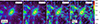 |
Fig. 1. High resolution convergence maps overlaid with reduced shear maps of an example cluster at z = 0.231 with M200 = 9.9 × 10¹⁴ M⊙. We show different lensing maps from left to right for source plane redshifts of zs = 0.8, 1.2, 2.0 and 3.0. For legibility, the reduced shear map has been down-sampled by a factor 30. At higher source redshifts, the gravitational lensing efficiency increases, but so does the amount of LoS structure. |
In a realistic cluster weak lensing analysis, source galaxy redshifts are distributed over a broad range, with the exact shape of the distribution depending on the specifics of the survey. This is captured in the source redshift distribution, n(zs), which we define such that ∫n(zs)dzs = 1. Given n(zs) and the lens redshift, the lensing efficiency can be computed with
 (7)
(7)
In weak lensing studies of clusters, the redshifts of the individual source galaxies are often not known. Therefore, it is common practice to adopt a single source plane approximation, in which all source galaxies are assumed to lie on a thin plane at an effective redshift, zeff. For low-redshift (zl ≲ 0.3) lenses, this effective source redshift is obtained by solving
 (8)
(8)
This ensures that the lensing efficiency of the approximated single source plane is equal to that of the real distribution of source redshifts.
3.2. Mock weak-lensing maps
In weak lensing, the dominant source of statistical noise is the intrinsic shape of the source galaxy. Following Bartelmann & Schneider (2001), the observed ellipticity1, ϵ for |g|< 1 is calculated as
 (9)
(9)
The intrinsic shape distribution of galaxies is well known, with a measured dispersion per component of σϵ = 0.26, hereafter referred to as ‘shape noise’. This value is derived from observations in the COSMOS (Leauthaud et al. 2007) and CANDELS (Schrabback et al. 2017) fields using the Hubble Space Telescope, with photometric properties similar to the Euclid VIS instrument. As a result, this value is widely adopted for modelling purposes within the Euclid Collaboration (e.g. Euclid Collaboration: Martinet et al. 2019; Euclid Collaboration: Ajani et al. 2023; Euclid Collaboration: Ingoglia et al. 2025) and adopted in this work.
Statistical uncertainty can be reduced by averaging over many galaxies in a given path of sky; however, this approach is ultimately limited by the number density of source galaxies. In this work, we assume a source galaxy number density of 30 galaxies per square arcminute, consistent with the expected depth of the Euclid survey (Euclid Collaboration: Mellier et al. 2025). For our assumed field of view, this corresponds to a total of 982 source galaxies. To incorporate this result, we down-sampled our high-resolution reduced shear maps using linear interpolation, placing the source galaxies on a uniform grid.
We constructed four types of mock weak-lensing maps to disentangle the effects of: (i) shortcomings of the assumed model; (ii) structure along the LoS; and (iii) statistical noise arising from the intrinsic shape of source galaxies. To study the dependence of source redshift on these effects, we assume single source planes at redshifts of 0.4, 0.8, 1.2, 1.6, 2.0, 2.4, and 3.0. For these source plane redshifts, we defined the following mocks:
-
CL: This mock isolates the intrinsic shortcomings of the modelling of the cluster’s mass density profile. It allows us to measure the intrinsic bias or scatter in a given model parameter. We did not add shape noise (σϵ = 0) and we used only a thin LoS shell of ±5 Mpc around the cluster, which excludes nearly all LoS structure. However, the width of this shell is still larger than the cluster itself and therefore includes part of the correlated LoS structure and its associated systematic uncertainties (see, e.g. Bahé et al. 2012).
-
CL+LoS: This mock isolates the systematic uncertainty introduced by LoS structure. It includes all structure along the LoS from the observer out to the source plane. No shape noise is included (σϵ = 0).
-
CL+σϵ: This mock isolates the statistical uncertainty due to shape noise. It includes only a thin LoS shell of ±5 Mpc around the cluster, while assuming shape noise of σϵ = 0.26.
-
CL+LoS+σϵ: This mock accounts for both systematic uncertainty due to LoS structure and statistical uncertainty due to shape noise. It includes structure along the full LoS and shape noise of σϵ = 0.26.
A central part of this paper is to quantify the impact of LoS structure on cluster weak lensing studies with upcoming Euclid data. To do so accurately, we must forward-model the source redshift distribution expected for Euclid, as provided by Euclid Collaboration: Mellier et al. (2025). To this end, we discretised this source redshift distribution into bins corresponding to the redshifts used in our single source plane mocks, assuming a fixed number of galaxies per bin. We then randomly associated every source galaxy on our uniform grid with a source redshift bin and assigned to it the reduced shear from the corresponding single source plane mock. In this way, we were able to construct a Euclid-like mock from a series of single source plane mocks. However, this procedure introduced stochasticity in our mocks, which we later marginalised over through a repeated resampling of the random assignment of source redshift bins to our sources. In this manner, we constructed two more Euclid-like mocks, which are representative for upcoming Euclid data:
-
Euclid+CL: This mock combines the CL+σϵ series of single source plane mocks into a mock with a source redshift distribution expected for Euclid. It includes shape noise of σϵ = 0.26, but no LoS structure. Instead, it includes only a thin LoS shell of ±5 Mpc around the cluster.
-
Euclid+CL+LoS: This mock combines the CL+σϵ+LoS series of single source plane mocks into a mock with a source redshift distribution expected for Euclid. It includes shape noise of σϵ = 0.26 and structure along the full LoS, which becomes varied in length from source galaxy to source galaxy.
To ensure the validity of our weak lensing formalism, we mask all source galaxies with κ > 0.9 and |g|> 1. This roughly follows the findings of Massey & Goldberg (2008), who demonstrated that the weak lensing approximation remains accurate to within a sub-percent level up to |g|≈0.93. The specifics of these mocks and their designators are summarised in Table 1.
Overview of our mock weak-lensing maps.
4. Modelling
In this section, we discuss how we measure the clusters, mass, concentration, axis ratio, and BCG wobble from our mock weak-lensing maps.
4.1. Mass density profile
In this work, we model the mass density profile of our simulated clusters with the NFW profile, an empirical model that accurately describes the mass density profiles of dark matter halos in N-body simulations (Navarro et al. 1996, 1997). Since the influence of LoS structure on the inferred density profile parameters depends on the choice of model, we consider both the spherically symmetric and the elliptical NFW mass density profile. The NFW profile has the asymptotic form of a broken power law. Under the assumption of spherical symmetry (sphNFW), it takes the form of
 (10)
(10)
where r is the radius, ρs is the characteristic density, and rs is the scale radius, which marks the transition from the r−1 to r−3 scaling of the density profile. The scale radius can be parametrised as a fraction 1/c200 of the halo’s R200, where c200 = R200/rs is the concentration. With these definitions the spherical NFW profile can be parametrised with four parameters: two for the centre, the mass M200, and the concentration c200.
Analytical expressions for the convergence and shear for the spherical NFW profile were written down for the first time in Bartelmann (1996). However, it is well established that dark matter halos are triaxial ellipsoidals (e.g. Jing & Suto 2002; Kasun & Evrard 2005; Allgood et al. 2006) and the assumption of spherical symmetry in lensing studies of galaxy clusters leads to biases of up to 40% on the mass (e.g. Feroz & Hobson 2011; Bahé et al. 2012; Herbonnet et al. 2022; Euclid Collaboration: Giocoli et al. 2024). It is therefore important for lensing studies to generalise the spherical NFW profile to an elliptical one (eNFW), and have expressions for the convergence and shear. Despite the apparent simplicity of the NFW profile, deriving the convergence and shear in the elliptical case has proven to be difficult.
Recently, the problem of convergence and shear for an eNFW profile has been solved analytically by Heyrovský & Karamazov (2024), by introducing ellipticity directly into the mass density profile. These analytical expressions give the exact convergence and shear emerging from an eNFW profile and at the same time allow for the kind of fast model evaluations required for Bayesian parameter inference. We refer to Heyrovský & Karamazov (2024) for the models detail. However, we note that we have modified the convention with which ellipticity is introduced. Specifically, we ensure that the enclosed mass in an iso-surface density contour stays constant for a changing axis ratio, q. This means we introduce ellipticity by changing coordinates from radius r to semi major axis, a, with the following coordinate transformation,
 (11)
(11)
Here, (x, y) are the Cartesian coordinates on the image, r(x, y) represents the magnitude of (x, y), and q is the axis ratio of the projected mass density profile.
The eNFW model of Heyrovský & Karamazov (2024) has six free parameters: (xc, yc), the Cartesian coordinates of the centre; q, the axis ratio of the projected mass density profile; ϕ, the orientation of the major axis with respect to the x-axis; as, the scale semi-major-axis; and κs, the halo convergence parameter. The parameter κs can be related to the characteristic density ρs of the 3D density profile, as, the critical density of the Universe, and a factor that depends on the 3D orientation of the ellipsoid with respect to the LoS; we refer to Equation (22) in Heyrovský & Karamazov (2024) for details on this. This model assumes a constant ellipticity for the dark matter halo, contrary to the demonstrated radial dependence of the ellipticity in simulated halos (e.g. Allgood et al. 2006; Schneider et al. 2012). We note that this is a simplifying assumption in this study, which can be improved upon in future works. Following the same reasoning as in the spherical case, we can swap as and κs for M200 and c200.
In this work, we employed both spherical and elliptical NFW models to measure mass and concentration and compare the results. In studies focussing on these parameters, the cluster centre is typically fixed by using a specific tracer. To maintain consistency with such studies and simplify our statistical analysis, we fix the centre at the position of the BCG (see Section 4.3 for details). This choice minimises biases from profile mis-centring, as collisionless dark matter simulations predict that the BCG’s offset from the potential centre is generally well below the softening length (Roche et al. 2024; Schaller et al. 2015). In observational studies, where the optimal tracer of the potential centre is uncertain, alternative choices include the X-ray centre, satellite distribution, or strong lensing data (e.g. von der Linden et al. 2014; Wang et al. 2018; Oguri et al. 2012).
Once the cluster’s centre is assumed, a choice must be made for the radial fitting range in the weak lensing analysis. An inner fitting radius is used to minimise the baryonic effects, while an outer radius helps mitigate the influence of large-scale structure. Previous studies have shown that the specific choice of these radii can introduce biases in weak lensing mass measurements (e.g. Becker & Kravtsov 2011; Bahé et al. 2012; Lee et al. 2018). In this work, we do not set an outer fitting radius due to the limited field of view, which extends only to R ∼ 2 Mpc. However, we masked all source galaxies within 30 arcsec of our assumed centre (the BCG) when inferring mass, concentration, and axis ratio. When applying the sphNFW model, we converted the relevant mock to reduced tangential shear.
To measure the BCG wobble we fit the full six-parameter eNFW model to the mocks. To maximise the sensitivity, we do not masked out the central region of the cluster. In this approach, we effectively marginalised over all other parameters in the eNFW model. A summary of the three different models that we use in this work is provided in Table 2.
Overview NFW models.
Our Euclid-like mocks include a realistic distribution of source galaxy redshifts, for which we assumed an effective source redshift in our modelling. Specifically, we solved Equation (8) for zl = 0.225 and n(zs) from Euclid Collaboration: Mellier et al. (2025), finding zeff = 0.60. While this procedure matches the average lensing efficiency of the full source redshift distribution, it still approximates all source galaxies to lie on a single source plane at z = zeff. This approximation can lead to additional bias in the inferred lensing signal due to the non-linear dependence of reduced shear on lensing efficiency. As a result, best-fit parameters (most notably mass) can receive additional bias from this simplification. Naturally, for the single source plane mocks, we assume perfect knowledge of the source plane redshift and take this value as input for our modelling.
4.2. Bayesian parameter estimation
We performed Bayesian parameter estimation with the fitting library of PyAutoLens (Nightingale et al. 2021). This is an open-source Python package originally developed for strong gravitational lensing with various features, such as (strong) lens modelling, (strong) lens simulations, and ray tracing. In this work we make use of its elaborate library designed for lens modelling. We make use of the NFWMCRScatterLudlow mass density profile, which samples the concentration, c200, as a number of ‘σc’ standard deviations (in units of dex) above or below the Ludlow et al. (2016) concentration mass relation, such that
 (12)
(12)
Here, c(M) is the Ludlow et al. (2016) concentration-mass relation and 0.15 is the standard deviation of the scatter in the concentration mass relation in units of dex (Wang et al. 2020).
The axis ratio and orientation of the major axis are sampled at the level of the decomposed ellipticity e = (ex, ey), which satisfies
 (13)
(13)
Within the framework of PyAutoLens, we used Nautilus (Lange 2023), which is a Python package designed for Bayesian posterior and evidence estimation. It improves on traditional Markov chain Monte Carlo (MCMC) methods by combining importance nested sampling (INS) (Feroz et al. 2019) with neural networks. For our model fits, we use 1000 live points. This choice provides a satisfactory balance between accuracy, precision and computational efficiency, as determined through tests with our mock data sets.
We adopted uniform priors except for M200, for which we adopt a log-uniform prior due to its wide dynamical range. This is common practice in cluster weak lensing studies (e.g. Sereno & Covone 2013; Umetsu et al. 2014; Umetsu 2020; Okabe et al. 2019) and planned for use in the Euclid cluster weak lensing program (e.g. Euclid Collaboration: Giocoli et al. 2024; Euclid Collaboration: Sereno et al. 2024; Euclid Collaboration: Ingoglia et al. 2025). Alternative choices, such as a uniform mass prior, can be made and would drive the inferred masses slightly upward. Due to computational constraints, we did not explore the interplay between the choice of mass prior and the effects of LoS structure. Thus, we restricted our study to a log-uniform mass prior. We acknowledge that our results may change if a uniform mass prior is assumed instead. The priors were defined within the following limits:
-
Mass density profile center: A square of width 50 arcsec (187 kpc at z = 0.225) centred on the BCG.
-
Mass: A range between 5 × 10¹³ M⊙ and 1 × 10¹⁶ M⊙.
-
Number of standard deviations above and below the Ludlow et al. (2016) concentration mass relation: A range of ±3 standard deviations.
-
Decomposed ellipticity: The full range of physically meaningful values: −1 < ex, y < 1.
A summary of these priors is listed in Table 2. In this study, we have aimed to quantify the impact of LoS structure on weak lensing observables of galaxy clusters in case no attempts were made to correct for them. In principle, we can mitigate its impact on the inferred precision by including non-diagonal terms in the covariance matrix, which are given by the two-point shear correlation function (see e.g. Oguri et al. 2010). However, we kept our covariance matrix diagonal and quantified the impact of LoS structure on the scatter. We note that including off-diagonal elements in the covariance matrix will not mitigate any biases induced by LoS structure that we present in this paper.
4.3. Brightest cluster galaxy
One aspect of this paper is to study the impact of LoS structure on the measured BCG wobble. These measurements rely on identification of two points: (i) the bottom of the gravitational potential, measured as the centre of the total mass density profile obtained through gravitational lensing; and (ii) the BCG centre, determined observationally from the peak of the stellar light distribution.
To determine the centre of the BCG, we generated surface density maps using stellar particles in the simulation. We did this by taking a thin shell of ±5 Mpc around the cluster in the light cone particle data and projecting all the particles on a 2D grid. This grid has a physical field-of-view of 1 Mpc and a resolution equal to the softening length, chosen so to keep the particle per pixel count sufficiently high. We assume that the stellar current particle masses trace the stellar light and use the resulting stellar surface density map as input for the peak-finding algorithm SExtractor (Bertin & Arnouts 1996). To improve the accuracy of the peak identification, we up-sampled the input maps through linear interpolation by a factor of 10 and applied a Gaussian filter with a standard deviation of 20 pixels. In the SExtractor output, we identified the source with the highest ‘flux’ (MAG_ISO) as the BCG and retrieved its centroid with the X_IMAGE and Y_IMAGE outputs.
5. Results
We studied the impact of LoS structure on weak lensing analyses of clusters, assuming the NFW profile variations outlined in Table 2. In the following, we compared the results of mass density profile reconstructions across the six mocks described in Table 1. For each single source plane mock, we performed a Bayesian parameter inference for mock setups with source plane redshifts of 0.8, 1.2, 1.6, 2.0, 2.4, and 3.0. Source redshifts below this range result in non-detections for low-mass clusters for mocks with non-zero shape noise, complicating faircomparisons between the samples. For the CL mock, the results are independent of source redshift due to the absence of both shape noise and LoS structure. Therefore, we performed the parameter inference on the CL mock only for a source plane redshift of 0.8 and used these results for all other source redshifts as well.
5.1. Residuals sphNFW fit on CL+LoS mock
To illustrate the effect of LoS structure on weak lensing observables, we first considered a simple case: fitting the sphNFW model to our CL+LoS mock. For each source redshift, we subdivided the sample into two groups based on whether the cluster lies along an over-dense or under-dense LoS. We assume that clusters along over-dense sight-lines have overestimated masses, while those along under-dense sight-lines have underestimated masses. Using mass bias as an estimator, we classify clusters with a mass bias below the sample median as ‘under-dense LoS’ and the rest as ‘over-dense LoS’.
To evaluate this subdivision, we examined the azimuthally averaged reduced tangential shear contribution from the LoS, hereafter  . To compute this quantity, we subtracted the CL mock from the CL+LoS mock, then averaged the result azimuthally in nine linear bins between 0.5 and 9 arcminutes.
The left panel of Figure 2 shows the median  profiles across our subsamples and source redshifts. Angular bins are converted to physical distances using the mean cluster redshift of z = 0.225. under-dense and over-dense LoS classifications are plotted in blue and red respectively, with varying shades representing different source redshifts. Our subdivision shows how over-dense and under-dense sight-lines are symmetrically distributed around zero. In other words, the median
  profile for the full sample is zero. This is expected, since an equal number of sight-lines pass through over-dense and under-dense regions of the Universe, causing their contributions to the median reduced tangential shear profile to average out to zero. The absolute value of the median
  profile increases with radius because the annular area grows, leading to greater variance in the projected mass density along the LoS. The absolute value of the median
  profile increases with source redshift as well, due to the longer LoS and boosted lensing efficiency.
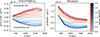 |
Fig. 2. Two subsamples resulting from the subdivision of the main sample, based on their having an over-dense (red) or under-dense (blue) LoS for a given source redshift (shaded colours). Left: Median azimuthally averaged reduced tangential shear contribution from the LoS, calculated as the difference between the reduced tangential shear from the CL+LoS mock and the CL mock, as a function of radius. Right: Median azimuthally averaged residuals, calculated as the difference between the reduced tangential shear from the best-fit model and the CL mock. On average, the residuals for clusters lying along over-dense and under-dense sight-lines are asymmetrically distributed around zero, potentially leading to a bias. |
In the right panel of Figure 2, we plot the median azimuthally averaged residuals as a function of radius for the under- and over-dense LoS subsamples. The residual is computed by subtracting the CL mock from the best-fit model. We find that over-dense LoS clusters consistently have overestimated profiles, with residuals increasing toward the centre. In contrast, under-dense LoS clusters have underestimated profiles at large radii but overestimated profiles in the inner regions.
Although the reduced tangential shear profile itself remains unbiased on average, the residuals of the under-dense and over-dense LoS subsamples are asymmetric around zero, potentially introducing biases in the inferred best-fit parameters. Physically, this suggests that the sphNFW profile provides a better fit for clusters along under-dense sight-lines than for those along over-dense sight-lines.
5.2. Mass, concentration, and axis ratio
In the previous section, we described how in the limit of infinite S/N, the sphNFW model provides a better fit for clusters along under-dense sight-lines than for those along over-dense ones. In this section, we quantify the resulting biases in the inferred cluster mass, concentration, and axis ratio. We also examine the scatter and the inferred precision of these parameters in relation to the effects of LoS structure.
We begin this discussion by considering our single source plane mocks to study the interplay between shape noise and LoS structure, and how this depends on source redshift. We first assess the impact on the best-fit parameters of the sphNFW model in Section 5.2.1, after which we discuss the same for the eNFW4 model in Section 5.2.2. Subsequently, we turn to our Euclid-like mocks to quantify the expected biases in cluster weak lensing analyses with Euclid data in Section 5.2.3. Finally, we discuss the estimated uncertainties on the free parameters of both models in Section 5.2.4.
5.2.1. Spherical NFW model
The sphNFW model has two free parameters: mass and concentration. As a ground truth for the mass and concentration we use the SOAP catalogued M200 and c200 from the simulation’s post-processing files2. SOAP calculates c200 using a slightly modified version of the method described by Wang et al. (2023), which estimates concentration based on the first-order moment of the mass density distribution, R1. This method uses a fifth-order polynomial fit to the R1-concentration relation for concentrations ranging between 1 and 1000. In Figure 3 we show the mean3 bias (top row) and scatter (bottom row) as a function of source redshift for the mass (left column) and concentration (right column) for our four mocks: CL+LoS (green-dashed), CL+σϵ (blue-dot-dashed), CL+LoS+σϵ (red-solid), and CL (black-dotted). We use the mean of the relative error distribution minus 1 as our estimator for the bias, while for scatter, we used the 16th and 84th percentiles of the relative error distributions, which are plotted as negative and positive values, respectively. Plotting the scatter in this manner allows us to observe any asymmetry induced in the relative error distributions. The error bars indicate the bootstrapped 1σ uncertainty on the mean or percentile.
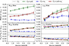 |
Fig. 3. Applying the sphNFW model we show the mean bias (top row) and scatter (bottom row) as a function of source redshift for the cluster’s mass (left column) and concentration (right column), for our four mocks CL (black-dotted), CL+LoS (green-dashed), CL+σϵ (blue-dot-dashed) and CL+LoS+σϵ (red-solid). We estimate the bias of quantity ‘𝒬’ as the mean of the relative error distribution minus 1. We estimate the upper bound scatter (+) and lower bound scatter (−) using the 84th and 16th percentile of the relative error distribution, respectively. |
In the upper panels of Figure 3, we observe that in our CL mock the sphNFW model intrinsically underestimates the mass and overestimates the concentration. This bias arises from projection effects: When a halo is observed along its major axis, the mass is overestimated, whereas projections along the other two axes underestimate it (e.g. Oguri & Hamana 2011; Bahé et al. 2012; Euclid Collaboration: Giocoli et al. 2024), leading to a net negative bias on average. The concentration compensates for this through the concentration-mass degeneracy, leading to an overestimated concentration. We refer to Oguri & Hamana (2011), for instance, for a more detailed discussion on this. It has been shown that this weak lensing mass bias can be reduced by fixing the concentration, either to a fixed value or via a theoretical concentration-mass relation (e.g. Lee et al. 2018; Euclid Collaboration: Giocoli et al. 2024). Furthermore, we observe that the intrinsic scatter in the mass is around a factor of two smaller than that in the concentration. This is a well-known result and can again be explained by projection effects.
The results from the CL+LoS mock in the bottom panels indicate that the intrinsic effect of LoS structure is to generate a positive skew in the relative error distributions for both mass and concentration. As a result, the mean biases in mass and concentration increase with source redshift.
This can be understood in context of the previous section, where we saw that the sphNFW model provides a better fit to clusters along under-dense sight-lines than those lying along over-dense ones. This leads to a model bias, whose quantitative effect on the mass and concentration we observe here. From the right panel of Figure 2 it is evident that the best-fit model is indeed overly concentrated on average.
With regards to the CL+σϵ mock, we observe that the scatter decreases slightly due to the boosted lensing efficiency between zs = 0.8 and zs = 3.0. Since there is no skew, we observe that both the mean mass and concentration biases do not vary with source redshift. We argue that the zs = 0.8 point for the mean concentration bias that breaks this trend is due to some low-S/N clusters with poorly constrained concentrations.
Aside from the presence of LoS structure, the key difference between these mocks is that the CL+LoS mock assumes an infinite S/N, whereas the CL+σϵ mock has a realistic one. As a result, in the CL+LoS mock, all radii contribute statistically, whereas in the CL+σϵ mock, the S/N drops below unity at a certain radius. Combined with the concentration-mass degeneracy, this leads to altered biases in mass and concentration.
We study the combined effects of realistic S/N and LoS structure using the CL+LoS+σϵ mock. We observe that the relative error distributions are skewed, similarly to the CL+LoS mock. Therefore, the mean mass and concentration biases follow a trend toward more positive biases as well. However, the effects of finite S/N changes its amplitude with respect to the CL+LoS mock. A comparison between the CL+σϵ and CL+σϵ+LoS mocks shows that LoS-induced biases in both mass and concentration persist under the assumption of realistic S/N. Further, we note that for zs ≳ 1.2, LoS structure dominates the upward scatter in the mass estimates. For the scatter in concentration the effects of LoS structure are less pronounced, indicating that other factors are likely more influential.
5.2.2. Elliptical NFW model
This subsection discusses the results for the eNFW4 model, which adds the axis ratio of the projected mass density profile as an additional degree of freedom. As a ground truth for the axis ratio, we used the axis ratio of the best-fit eNFW4 model on 2 arcsec resolution convergence maps. Similarly to Figure 3, Figure 4 shows the mean4 bias and scatter for mass, concentration and axis ratio as a function of source redshift across our four mocks.
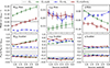 |
Fig. 4. Same as Figure 3, but employing the eNFW4 model, which treats the axis ratio (q) as a free parameter (right column). |
Here, we discuss the results on the mass and concentration. The CL mock demonstrates that, compared to the sphNFW model, the mean concentration bias decreases by ∼20% point, while the absolute median mass bias shows a slight reduction. This suggests that projection effects are partially mitigated by the added flexibility of the eNFW4 model.
For the CL+LoS mock, we observe trends that closely mirror those found for the sphNFW model. However, in this case, we find that the skew in the relative error distribution is even stronger, especially in the mass. Similarly, the CL+σϵ mock shows trends consistent with the sphNFW model, with both the mean mass and concentration biases roughly constant with source redshift. Comparing the mean mass bias in the CL+σϵ and CL+LoS+σϵ mocks, we observe that LoS structure induces additional bias, consistent with our findings for the sphNFW model. In contrast, for the concentration, we now see no significant bias resulting from the effects of LoS structure. This highlights that the biases associated with LoS structure can be model dependent.
Regarding the scatter, we observe an overall decrease compared to the sphNFW model, which again relates back to the partial modelling of halo triaxiality. As with the sphNFW model, LoS structure dominates the positive scatter in mass for zs ≳ 1.2, while its effect on concentration scatter is weaker, likely due to other dominant factors.
Moving on to the right most column, we observe for the axis ratio that LoS structure biases this measurement low, meaning clusters appear more elliptical than they truly are. This can be understood, as halos along the LoS, projected in the cluster’s outskirts, will elongate the best fit mass model in order to account for their signal. On the other hand, the LoS contributes minimally to the scatter in the measured axis ratio.
5.2.3. Euclid-like mock data
In the previous sections we have seen that LoS structure can lead to additional bias in parameter inference, with the magnitude of this bias increasing with source redshift. A key simplification in the mocks we considered is the assumption of single source planes. Next, we want to take into account the source redshift distribution expected for Euclid, to quantify the significance of LoS-induced biases for upcoming Euclid data. Toward this end, we study our Euclid-like mocks (Euclid+CL and Euclid+CL+LoS), which have sources randomly sampled from the expected source redshift distribution for Euclid, as provided by Euclid Collaboration: Mellier et al. (2025) (see Section 3.2 for details). In the modelling of the cluster’s lensing signal, we assume an effective source redshift of zeff = 0.6 (see the end of Section 4.1 for details).
By randomly sampling the redshift of the sources on our uniform grid, we introduce stochasticity in our analysis. We marginalise over this stochasticity by rerunning our Bayesian inference 10 times for each cluster, each time resampling the source redshifts. We then report the mean best-fit parameters over these 10 inferences for the remainder of our analysis. We have verified that increasing this number to 20 times does not significantly affect our results in fitting the sphNFW model to the Euclid+CL+LoS mock.
In Figure 5, we plot the resulting relative error distributions of our model free parameters for the Euclid+CL mock in purple and the Euclid+CL+LoS mock in orange. In the large panel on the left, we show the relative error distribution for the mass, estimated by assuming the sphNFW model, which is a common approach in cluster weak lensing studies. In the right panels, we present (from left to right and top to bottom) the relative error distributions for: the concentration estimated with the sphNFW model, followed by the concentration, mass, and axis ratio estimated with the eNFW4 model. In all panels, we show zero (black and dotted) and the difference in mean bias, Δμ, with the bootstrapped 1σ uncertainty.
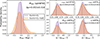 |
Fig. 5. Relative error distributions for the best-fit parameters in the Euclid+CL (purple) and Euclid+CL+LoS (orange) mocks. We show the relative error distribution for mass (left panel); concentration (right panel: top-left) under the assumption of the sphNFW model; and mass (right panel: bottom-left); concentration (right panel: top-right); and axis ratio (right panel: bottom-right) under the assumption of the eNFW4 model. We report the difference of the means (Δμ) and it’s bootstrapped uncertainty on the top right of each panel. For Euclid-like data, LoS structure positively biases mass estimates with the sphNFW model on the level of +5.3 ± 1.4%, which is significant at 3.5σ. |
As we discussed in previous sections, we observe in the left panel that LoS structure induces a positive skew in the relative error distribution of the mass estimated with the sphNFW model. This results in a positive mean mass bias +5.3 ± 1.4%, which is significant at 3.5σ. When the mass is estimated with the eNFW4 model, the mean mass bias associated with LoS structure increases to +6.1 ± 1.3%, which is significant at 4.7σ. In these mocks, the concentration is not biased significantly by LoS structure. As seen before, the scatter in concentration is much larger than in the mass, relegating the effects of LoS structure to a subdominant level. Moving on to the axis ratio, we observe that LoS structure biases these measurements, lowering them by −2.0 ± 0.7% on average, which is significant at 2.9σ. As expected, the results for these mocks are roughly consistent with what we observed for comparing the single source plane mocks CL+σϵ and CL+LoS+σϵ at zs = 0.8. These results demonstrate that, for cluster weak lensing analyses with Euclid data, the impact of LoS structure must be incorporated into the error budget to avoid significant biases in cluster mass and shape estimates.
5.2.4. Inferred precision
Having established that, at least for the mass, LoS structure contributes significantly to the scatter, we need to investigate whether this is accounted for in the estimated uncertainty as derived during the fit by Nautilus. Note that we have not included the effects of LoS structure in the covariance matrix, which would help estimate the true uncertainty. To do this, we compute the mean 84th percentile of the Bayesian-inferred relative uncertainty from the CL+LoS+σϵ and Euclid+CL+LoS mocks. The results are shown in Figure 6, where the CL+LoS+σϵ mock is represented by red dashed lines, and the Euclid+CL+LoS mock by orange stars. We compare this estimated uncertainty to the 84th percentile of the true relative error distribution, represented by red dashed lines and orange crosses for CL+LoS+σϵ and Euclid+CL+LoS mocks, respectively. The top panels show this comparison for the mass and concentration estimated with the sphNFW model, while the bottom panels show this comparison for the mass, concentration and axis ratio estimated with the eNFW4 model. Additionally, we plot in gray dotted a curve proportional to the critical surface density, which is inversely proportional to the lensing efficiency at fixed lens redshift.
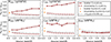 |
Fig. 6. Comparison of the estimated uncertainty (Nautilus, diagonal covariance matrix) and true scatter (84th percentile relative error distribution). The top panels show the results for the free parameters of the sphNFW model, while the bottom panels show the same for the eNFW4 model. For the CL+LoS+σϵ mock, the estimated uncertainty and true scatter are shown as red-dashed and red-solid lines, respectively. For the Euclid+CL+LoS mock, the estimated uncertainty and true scatter are shown in orange stars and crosses, respectively. A gray-dotted curve indicates a quantity inversely proportional to the lensing efficiency. Under the assumption of a diagonal covariance matrix, LoS-induced scatter in mass estimates is not accounted for in the Bayesian parameter inference. |
For the mass estimated by both models, we observe that the true scatter increases with source redshift, driven by LoS structure (as discussed in Sections 5.2.1 and 5.2.2). In contrast, the estimated uncertainty decreases with source redshift, inversely proportional to the lensing efficiency. This indicates that, under the assumption of a diagonal covariance matrix, LoS-induced uncertainties in mass estimates are not taken into account in the posterior distributions. The Euclid+CL+LoS mock shows that this effect is subdominant for upcoming Euclid data. However, for future, deeper, weak lensing surveys (e.g. the Nancy Grace Roman Space Telescope Spergel et al. 2015; Akeson et al. 2019, scheduled for launch in 2027), this effect needs to be taken into account to avoid overestimating the precision on the mass.
Regarding the concentration, we observe a large overestimation of precision for both mocks and models. However, as discussed in Sections 5.2.1 and 5.2.2, the large scatter in concentration is not driven by LoS structure, but by other systematics such as projection effects. Therefore, this overestimation of precision in concentration is an issue separate from LoS structure that needs to be addressed in future work. Regarding the axis ratio, we observe only small differences between true scatter and estimated uncertainty.
5.3. Brightest cluster galaxy wobble
Structure along the LoS can induce mis-centring, biasing the measured offsets between the bottom of the gravitational potential and the brightest cluster galaxy (BCG), known as the BCG wobble. This subsection is dedicated to quantifying this effect relative to the statistical uncertainties introduced by shape noise. As discussed in Section 4, we infer the bottom of the gravitational potential by applying the eNFW6 model to the relevant mock. We plot the median BCG wobble measured in our samples as a function of source redshift in Figure 7. We show the results for the CL, CL+LoS, CL+σϵ and CL+LoS+σϵ single source plane mocks in the black-dotted, red-dashed, blue-dot-dashed and purple-solid curves, respectively. Additionally, we plot the results for the Euclid+CL and Euclid+CL+LoS mocks in purple and orange crosses, respectively.
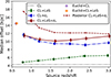 |
Fig. 7. Median offset between the centre of the gravitational potential and the BCG (BCG wobble) as a function of source redshift for: the CL (black-dotted), CL+LoS (green-dashed), CL+σϵ (blue-dot-dashed), CL+LoS+σϵ (red-solid), Euclid+CL (purple-cross) and Euclid+CL+LoS (orange-cross) mocks. The error bars indicate the 1σ bootstrapped uncertainty. The red dashed line indicates the median wobble as expected from random sampling the posterior distribution for the centre on the CL+LoS+σϵ mock. For upcoming Euclid data, measured median offsets of ∼14 kpc are expected for cold dark matter, with no significant contribution of LoS structure. |
We first analyse the CL and CL+LoS mocks to assess the intrinsic impact of LoS structure on BCG wobble measurements. For the CL mock, we find a median BCG wobble of 4 kpc. Given that the high-resolution FLAMINGO run has a softening length of 2.85 kpc (for z < 2.91), and that cold dark matter simulations predict offsets between the dark matter centroid and BCG to be smaller than the simulation’s softening length (Roche et al. 2024; Schaller et al. 2015), this result may seem unexpected. However, the lower offsets found by these studies can be attributed to their assumption of an idealised scenario in which the cluster’s mass distribution is perfectly known. In contrast, our result stems from biases in the eNFW6 model, which arise from assumptions such as axisymmetry, as well as the observational limitation of a finite number of source galaxies. The CL+LoS mock demonstrates that the median BCG wobble increases with source plane redshift. This trend can be attributed to LoS-induced mis-centring of the mass density profile, indicating that in the limit of infinite S/N, LoS structure biases the BCG wobble measurements.
Next, we measure the BCG wobble in the CL+σϵ and CL+LoS+σϵ mocks to study the impact of LoS structure on measurements with a realistic S/N. It is evident that introducing shape noise causes the median offset to increase substantially, due to the increased statistical uncertainty in the mocks. In the CL+σϵ mock, we observe that the measured BCG wobbles decrease as a function of source redshift. This trend can be attributed to the increasing lensing efficiency at higher redshifts, which boosts the S/N. For the CL+LoS+σϵ mock, we find that the median offset initially decreases due to increased lensing efficiency, but then rises again due to the larger number of LoS structures at higher source redshifts. The Euclid+CL and Euclid+CL+LoS mocks show, however, that the bias associated with LoS structure can be completely neglected for upcoming Euclid data. We note that the median offsets for these mocks are unexpectedly high considering the zs = 0.8 single source plane mocks. This is due to poor sampling of the redshift distribution of source galaxies at small radii, where the offset measurements are most sensitive to. By marginalising over this effect in our mocks we introduce an additional source of statistical error, which further increases the measured median offsets.
Next, we investigate whether the LoS-induced uncertainty in the CL+LoS+σϵ+LoS mock is properly accounted for in the estimated posterior distributions of the Bayesian parameter inference. To this end, we computed the median wobble under the assumption that the bottom of potential and BCG coincide. In which case, the median offset depends solely on the uncertainty in the mass density profile centre. The magnitude of a 2D vector with normally distributed components follows a Rayleigh distribution, whose median is given by  , where σcomp is the standard deviation of the normally distributed vector components. Assuming that the posterior distributions for both components of the centre are normally distributed and, on average, identical, we can estimate the median wobble using this expression. The result is shown as the dashed red line in Figure 7. This shows that the uncertainty estimate on the BCG wobble tends towards underestimating the true uncertainty. This indicates that any detection of a significant BCG wobble with weak lensing will be robust.
6. Conclusions
We quantified the impact of LoS structure on the recovery of mass density profile parameters from weak lensing studies of galaxy clusters. Using the highest-resolution FLAMINGO simulation (L1_m8; Schaye et al. 2023), we constructed a sample of 967 clusters with M200 > 3 × 10¹⁴ M⊙ and 0.20 < z < 0.25. We generated several mock weak-lensing maps, with a source galaxy number density of 30 galaxies/arcmin2, consistent with expectations for the Euclid survey.
To study the interplay between LoS structure and shape noise, while also examining how this evolves with source redshift, we constructed four single source plane mocks. Additionally, we assess the significance of LoS effects for upcoming Euclid data by constructing two more mocks with a realistic Euclid-like source redshift distribution (see Table 1). We performed Bayesian parameter inference with Nautilus (Lange 2023) using three versions of the NFW mass density profile to recover mass density profile parameters. For determining the mass, concentration, and axis ratio of the projected mass distribution, we use both spherical and elliptical NFW models (sphNFW and eNFW4; see Table 2), fixing the centre at the position of the brightest cluster galaxy (BCG). To determine the bottom of the gravitational potential (and thereby measuring the BCG wobble), we applied a six-parameter elliptical NFW model (eNFW6; see Table 2). From our analysis, we concluded the following:
-
In the limit of infinite S/N, we find that the median azimuthally averaged reduced tangential shear profile remains unbiased by LoS structure, meaning that the average profile is unaffected by variations in the LoS contribution (left panel of Figure 2). However, the residuals from fitting a spherical NFW (sphNFW) indicate that it provides a better fit for clusters along under-dense sight-lines than for those along over-dense ones (right panel of Figure 2), introducing a model bias. Indeed, as seen in Figure 3, increasing the source plane distance extends the LoS, generating a positive skew in the relative error distribution, and a resulting positive bias in both mass and concentration. These trends persist under the assumption of a realistic S/N (although to a lesser extent for the concentration). Regarding the elliptical NFW model, the same trends hold for the mass, although the bias in concentration largely disappears, highlighting the model dependence of these biases (Figure 4).
-
Comparing two mocks representative of upcoming Euclid data, we conclude that LoS structure induces an additional mass bias of 5.3 ± 1.4%, when adopting the commonly used spherical NFW model (see left panel Figure 5). This bias is statistically significant at the 3.5σ level, highlighting its importance for accurate weak lensing masses. This mean mass bias increases further to 6.1 ± 1.3% under the assumption of an elliptical NFW model. The concentration however, remains unbiased by LoS structure for both models with large scatter due to other contributing factors (right panels Figure 5). Our conclusions regarding the sphNFW model contrast with previous findings for the weak lensing mass bias by Hoekstra et al. (2011) and Becker & Kravtsov (2011). However, we note that Hoekstra et al. (2011) assumed that clusters follow a perfect sphNFW profile, which differs significantly from the simulated clusters in this study. Additionally, Becker & Kravtsov (2011) considered a maximum LoS length of only 400 h−1 Mpc, which may have been too short for this bias to manifest clearly.
-
For source redshifts, zs ≳ 1.2, the effects of LoS structure dominate the upper bound scatter in mass (see bottom rows of Figures 3 and 4). When a diagonal covariance matrix is assumed, Nautilus fails to capture this additional scatter, resulting in an overestimation of the inferred precision (see Figure 6). Our mocks, which aimed at being representative of upcoming Euclid data, show that this effect will be subdominant for cluster weak lensing studies with Euclid (see Figure 6). However, for future surveys with state-of-the-art instruments, such as the Nancy Grace Roman Space Telescope (Spergel et al. 2015; Akeson et al. 2019), which will produce significantly deeper weak lensing data, this effect will have to be taken into account. For the scatter in concentration, we find that LoS structure plays a subdominant role compared to other factors, such as projection effects.
-
The structure along the LoS leads to an underestimation of the projected mass density profile’s axis ratio, without significantly increasing the scatter (see Figure 4). For mocks that are representative of upcoming Euclid data, this bias amounts to −2.0 ± 0.7%, which is significant at 2.9σ (see Figure 5). This bias should be considered in studies using weak lensing measurements of halo ellipticity as a probe for self-interacting dark matter. Neglecting it could result in an underestimation of the halo’s true roundness and, consequently, a loss of constraining power in the self-interaction cross-section of dark matter.
-
Structure along the LoS can lead to the mis-centring of the mass density profile, potentially biasing the median measured offset of the BCG from the potential centre (BCG wobble). For our single source plane mocks, this bias is only significant for high source redshifts, zs ≳ 2. Our mocks with a realistic Euclid-like source redshift distribution show that the effects of LoS structure are negligible compared to other sources of (statistical) uncertainty. Additionally, the dark matter self-interaction cross-section has been constrained through observations of the offsets between galaxies and the centre of the gravitational potential in merging clusters (see e.g. Randall et al. 2008; Harvey et al. 2015; Sirks et al. 2024). While we have not specifically analyzed BCG offsets from the bottom of the potential in merging clusters, we argue that our conclusions are still relevant in these cases.
-
We forward-modelled measurements of the median BCG wobble with Euclid weak lensing data. Our results suggest that a measured offset of ∼14 kpc is still consistent with cold dark matter (see Figure 7). In this measured offset, the leading contributing factor is shape noise, with a small contribution from the sampling of the source redshifts at small radii. Moreover, we have shown that the Bayesian-inferred posterior for the mass density profile centre, tends to underestimate the true precision. This means that any statistically significant detection of a BCG wobble with weak lensing will be robust.
It is important to note that our choice of spatial distribution of source galaxies is a simplification. In reality, source galaxies are clustered and correlated with the LoS structure considered in this paper. This higher order effect is not considered in this work, but it has been deemed negligible compared to statistical noise in Hoekstra et al. (2011). Additionally, improvements could be made on the eNFW model by allowing the axis ratio of the projected mass density profile to vary with radius, providing a more realistic description of dark matter halo shapes.
In summary, we have shown that LoS structure can introduce significant systematic uncertainty in weak lensing studies of galaxy clusters. While the average lensing signal of clusters remains unbiased, the inferred parameters are still susceptible to biases. This occurs because the NFW models used in this study provide a better fit for clusters along under-dense sight lines than those along over-dense ones. Most notably, we find that in Euclid-like mock data, the LoS structure induces significant biases in cluster mass and shape estimates. Looking ahead, we predict that for future missions such as the Nancy Grace Roman Space Telescope, LoS structure will become the dominant source of scatter in cluster weak-lensing mass estimates. Assuming a diagonal covariance matrix in such analyses will then lead to a significantly overestimation of the precision.
As demonstrated in this work, future weak lensing studies of galaxy clusters striving for a high level of precision and accuracy must test their methods against the effects of LoS structure and include these effects in their error budgets. Therefore, we advocate for the use of cosmological simulations with sufficient light-cone output to self-consistently model the effects along the full LoS in the calibration of cluster weak-lensing pipelines.
Where we use the convention that |ϵ|=(a − b)/(a + b), where a and b are the major and minor axes of the ellipse, respectively.
SOAP was run on the simulation snapshots, cataloguing cluster properties at either z = 0.20 or z = 0.25, depending on which is closer. Considering the elapsed time between z = 0.225 and z = 0.200 (approximately equal to the time between z = 0.250 and z = 0.225), and using the average halo accretion rate of Correa et al. (2015b), we estimate that the halo mass changes by ∼2%. Since the sample’s redshift distribution is uniform, this will not lead to a bias, since half of the clusters will have slightly overestimated masses, while the other half will be slightly underestimated. This effect contributes minimally to the scatter, with a maximum impact of ∼2%, rendering it subdominant. Given the small change in mass, we expect the change in concentration to be subdominant as well.
Acknowledgments
This work was supported by the Swiss State Secretariat for Education, Research and Innovation (SERI) under contract number 521107294. The authors would like to thank John Helly and Roi Kugel for their role in the FLAMINGO project, which made this study possible. This work used the DiRAC@Durham facility managed by the Institute for Computational Cosmology on behalf of the STFC DiRAC HPC Facility (www.dirac.ac.uk). The equipment was funded by BEIS capital funding via STFC capital grants ST/K00042X/1, ST/P002293/1, ST/R002371/1 and ST/S002502/1, Durham University and STFC operations grant ST/R000832/1. DiRAC is part of the National e-Infrastructure. JWN is supported by an STFC/UKRI Ernest Rutherford Fellowship, Project Reference: ST/X003086/1.
References
- Abbott, T., Aguena, M., Alarcon, A., et al. 2022, Phys. Rev. D, 105, 023520 [NASA ADS] [CrossRef] [Google Scholar]
- Akeson, R., Armus, L., Bachelet, E., et al. 2019, ArXiv e-prints [arXiv:1902.05569] [Google Scholar]
- Allen, S. W., Rapetti, D. A., Schmidt, R. W., et al. 2007, MNRAS, 383, 879 [CrossRef] [Google Scholar]
- Allgood, B., Flores, R. A., Primack, J. R., et al. 2006, MNRAS, 367, 1781 [NASA ADS] [CrossRef] [Google Scholar]
- Bahé, Y. M., McCarthy, I. G., & King, L. J. 2012, MNRAS, 421, 1073 [NASA ADS] [CrossRef] [Google Scholar]
- Bartelmann, M. 1996, A&A, 313, 697 [NASA ADS] [Google Scholar]
- Bartelmann, M., & Schneider, P. 2001, Phys. Rep., 340, 291 [Google Scholar]
- Becker, M. R., & Kravtsov, A. V. 2011, ApJ, 740, 25 [NASA ADS] [CrossRef] [Google Scholar]
- Bernstein, G., & Huterer, D. 2010, MNRAS, 401, 1399 [Google Scholar]
- Bertin, E., & Arnouts, S. 1996, A&AS, 117, 393 [NASA ADS] [CrossRef] [EDP Sciences] [Google Scholar]
- Braspenning, J., Schaye, J., Schaller, M., et al. 2024, MNRAS, 533, 2656 [NASA ADS] [CrossRef] [Google Scholar]
- Broxterman, J. C., Schaller, M., Hoekstra, H., et al. 2025, MNRAS, 538, 755 [Google Scholar]
- Bryan, S. E., Kay, S. T., Duffy, A. R., et al. 2013, MNRAS, 429, 3316 [Google Scholar]
- Chen, Z., & Yu, Y. 2024, MNRAS, 534, 1205 [Google Scholar]
- Child, H. L., Habib, S., Heitmann, K., et al. 2018, ApJ, 859, 55 [NASA ADS] [CrossRef] [Google Scholar]
- Correa, C. A., Wyithe, J. S. B., Schaye, J., & Duffy, A. R. 2015a, MNRAS, 452, 1217 [CrossRef] [Google Scholar]
- Correa, C. A., Wyithe, J. S. B., Schaye, J., & Duffy, A. R. 2015b, MNRAS, 450, 1521 [NASA ADS] [CrossRef] [Google Scholar]
- Debackere, S. N. B., Schaye, J., & Hoekstra, H. 2021, MNRAS, 505, 593 [NASA ADS] [CrossRef] [Google Scholar]
- Donahue, M., Ettori, S., Rasia, E., et al. 2016, ApJ, 819, 36 [Google Scholar]
- Eckert, D., Ettori, S., Coupon, J., et al. 2016, A&A, 592, A12 [NASA ADS] [CrossRef] [EDP Sciences] [Google Scholar]
- Ettori, S., Morandi, A., Tozzi, P., et al. 2009, A&A, 501, 61 [NASA ADS] [CrossRef] [EDP Sciences] [Google Scholar]
- Ettori, S., Donnarumma, A., Pointecouteau, E., et al. 2013, Space Sci. Rev., 177, 119 [Google Scholar]
- Euclid Collaboration (Martinet, N., et al.) 2019, A&A, 627, A59 [NASA ADS] [CrossRef] [EDP Sciences] [Google Scholar]
- Euclid Collaboration (Scaramella, R., et al.) 2022, A&A, 662, A112 [NASA ADS] [CrossRef] [EDP Sciences] [Google Scholar]
- Euclid Collaboration (Ajani, V., et al.) 2023, A&A, 675, A120 [NASA ADS] [CrossRef] [EDP Sciences] [Google Scholar]
- Euclid Collaboration (Giocoli, C., et al.) 2024, A&A, 681, A67 [NASA ADS] [CrossRef] [EDP Sciences] [Google Scholar]
- Euclid Collaboration (Sereno, M., et al.) 2024, A&A, 689, A252 [NASA ADS] [CrossRef] [EDP Sciences] [Google Scholar]
- Euclid Collaboration (Ingoglia, L., et al.) 2025, A&A, 695, A280 [Google Scholar]
- Euclid Collaboration (Mellier, Y., et al.) 2025, A&A, 697, A1 [Google Scholar]
- Ferlito, F., Davies, C. T., Springel, V., et al. 2024, MNRAS, 533, 3209 [Google Scholar]
- Feroz, F., & Hobson, M. P. 2011, MNRAS, 420, 596 [Google Scholar]
- Feroz, F., Hobson, M. P., Cameron, E., & Pettitt, A. N. 2019, OJA, 2, 10 [Google Scholar]
- Giocoli, C., Despali, G., Meneghetti, M., et al. 2025, A&A, 697, A184 [NASA ADS] [CrossRef] [EDP Sciences] [Google Scholar]
- Grandis, S., Bocquet, S., Mohr, J. J., Klein, M., & Dolag, K. 2021, MNRAS, 507, 5671 [NASA ADS] [CrossRef] [Google Scholar]
- Han, J., Cole, S., Frenk, C. S., Benitez-Llambay, A., & Helly, J. 2017, MNRAS, 474, 604 [Google Scholar]
- Harvey, D., Massey, R., Kitching, T., Taylor, A., & Tittley, E. 2015, Science, 347, 1462 [Google Scholar]
- Harvey, D., Courbin, F., Kneib, J. P., & McCarthy, I. G. 2017, MNRAS, 472, 1972 [CrossRef] [Google Scholar]
- Harvey, D., Robertson, A., Massey, R., & McCarthy, I. G. 2019, MNRAS, 488, 1572 [NASA ADS] [CrossRef] [Google Scholar]
- Harvey, D., Robertson, A., Tam, S.-I., et al. 2021, MNRAS, 500, 2627 [Google Scholar]
- Herbonnet, R., Crawford, A., Avestruz, C., et al. 2022, MNRAS, 513, 2178 [NASA ADS] [CrossRef] [Google Scholar]
- Heyrovský, D., & Karamazov, M. 2024, A&A, 690, A19 [NASA ADS] [CrossRef] [EDP Sciences] [Google Scholar]
- Hoekstra, H. 2001, A&A, 370, 743 [NASA ADS] [CrossRef] [EDP Sciences] [Google Scholar]
- Hoekstra, H. 2003, MNRAS, 339, 1155 [NASA ADS] [CrossRef] [Google Scholar]
- Hoekstra, H., & Jain, B. 2008, Annu. Rev. Nucl. Part. Sci., 58, 99 [NASA ADS] [CrossRef] [Google Scholar]
- Hoekstra, H., Hartlap, J., Hilbert, S., & van Uitert, E. 2011, MNRAS, 412, 2095 [NASA ADS] [CrossRef] [Google Scholar]
- Hoekstra, H., Herbonnet, R., Muzzin, A., et al. 2015, MNRAS, 449, 685 [NASA ADS] [CrossRef] [Google Scholar]
- Jing, Y. P., & Suto, Y. 2002, ApJ, 574, 538 [Google Scholar]
- Kaiser, N., & Squires, G. 1993, ApJ, 404, 441 [Google Scholar]
- Kasun, S. F., & Evrard, A. E. 2005, ApJ, 629, 781 [NASA ADS] [CrossRef] [Google Scholar]
- Kim, S. Y., Peter, A. H. G., & Wittman, D. 2017, MNRAS, 469, 1414 [NASA ADS] [CrossRef] [Google Scholar]
- Kugel, R., Schaye, J., Schaller, M., et al. 2023, MNRAS, 526, 6103 [NASA ADS] [CrossRef] [Google Scholar]
- Lange, J. U. 2023, MNRAS, 525, 3181 [NASA ADS] [CrossRef] [Google Scholar]
- Laureijs, R., Amiaux, J., Arduini, S., et al. 2011, ArXiv e-prints [arXiv:1110.3193] [Google Scholar]
- Leauthaud, A., Massey, R., Kneib, J., et al. 2007, ApJS, 172, 219 [NASA ADS] [CrossRef] [Google Scholar]
- Lee, B. E., Le Brun, A. M. C., Haq, M. E., et al. 2018, MNRAS, 479, 890 [Google Scholar]
- López-Cano, D., Angulo, R. E., Ludlow, A. D., et al. 2022, MNRAS, 517, 2000 [CrossRef] [Google Scholar]
- Ludlow, A. D., Bose, S., Angulo, R. E., et al. 2016, MNRAS, 460, 1214 [Google Scholar]
- Ludlow, A. D., Schaye, J., & Bower, R. 2019, MNRAS, 488, 3663 [Google Scholar]
- Mandelbaum, R., Rowe, B., Bosch, J., et al. 2014, ApJS, 212, 5 [Google Scholar]
- Massey, R., & Goldberg, D. M. 2008, ApJ, 673, L111 [Google Scholar]
- McGibbon, R., Helly, J. C., Schaye, J., Schaller, M., & Vandenbroucke, B. 2025, JOSS, 10, 8252 [Google Scholar]
- Metzler, C. A., White, M., & Loken, C. 2001, ApJ, 547, 560 [NASA ADS] [CrossRef] [Google Scholar]
- Miralda-Escude, J. 2002, ApJ, 564, 60 [Google Scholar]
- Moreno, V. J. F., Helly, J., McGibbon, R., et al. 2025, ArXiv e-prints [arXiv:2502.06932] [Google Scholar]
- Navarro, J. F., Frenk, C. S., & White, S. D. M. 1996, ApJ, 462, 563 [Google Scholar]
- Navarro, J. F., Frenk, C. S., & White, S. D. M. 1997, ApJ, 490, 493 [Google Scholar]
- Nightingale, J., Hayes, R., Kelly, A., et al. 2021, JOSS, 6, 2825 [NASA ADS] [CrossRef] [Google Scholar]
- Niikura, H., Takada, M., Okabe, N., Martino, R., & Takahashi, R. 2015, PASJ, 67, 103 [NASA ADS] [CrossRef] [Google Scholar]
- Oguri, M., & Hamana, T. 2011, MNRAS, 414, 1851 [NASA ADS] [CrossRef] [Google Scholar]
- Oguri, M., Takada, M., Okabe, N., & Smith, G. P. 2010, MNRAS, 405, 2215 [NASA ADS] [Google Scholar]
- Oguri, M., Bayliss, M. B., Dahle, H., et al. 2012, MNRAS, 420, 3213 [Google Scholar]
- Okabe, N., Oguri, M., Akamatsu, H., et al. 2019, PASJ, 71, 79 [Google Scholar]
- Randall, S. W., Markevitch, M., Clowe, D., Gonzalez, A. H., & Bradač, M. 2008, ApJ, 679, 1173 [NASA ADS] [CrossRef] [Google Scholar]
- Refregier, A., Kacprzak, T., Amara, A., Bridle, S., & Rowe, B. 2012, MNRAS, 425, 1951 [Google Scholar]
- Rines, K., Geller, M. J., Diaferio, A., & Kurtz, M. J. 2013, ApJ, 767, 15 [NASA ADS] [CrossRef] [Google Scholar]
- Robertson, A., Huff, E., & Markovič, K. 2023, MNRAS, 521, 3172 [Google Scholar]
- Roche, C., McDonald, M., Borrow, J., et al. 2024, OJA, 7, 65 [Google Scholar]
- Schaller, M., Robertson, A., Massey, R., Bower, R. G., & Eke, V. R. 2015, MNRAS, 453, L58 [Google Scholar]
- Schaller, M., Borrow, J., Draper, P. W., et al. 2024, MNRAS, 530, 2378 [NASA ADS] [CrossRef] [Google Scholar]
- Schaye, J., Kugel, R., Schaller, M., et al. 2023, MNRAS, 526, 4978 [NASA ADS] [CrossRef] [Google Scholar]
- Schneider, M. D., Frenk, C. S., & Cole, S. 2012, JCAP, 2012, 030 [CrossRef] [Google Scholar]
- Schrabback, T., Applegate, D., Dietrich, J. P., et al. 2017, MNRAS, 474, 2635 [Google Scholar]
- Sereno, M., & Covone, G. 2013, MNRAS, 434, 878 [Google Scholar]
- Sirks, E. L., Harvey, D., Massey, R., et al. 2024, MNRAS, 530, 3160 [Google Scholar]
- Spergel, D., Gehrels, N., Baltay, C., et al. 2015, ArXiv e-prints [arXiv:1503.03757] [Google Scholar]
- Springel, V., White, S. D. M., Jenkins, A., et al. 2005, Nature, 435, 629 [Google Scholar]
- Umetsu, K. 2020, A&ARv, 28, A7 [Google Scholar]
- Umetsu, K., Medezinski, E., Nonino, M., et al. 2014, ApJ, 795, 163 [NASA ADS] [CrossRef] [Google Scholar]
- Varga, T. N., DeRose, J., Gruen, D., et al. 2019, MNRAS, 489, 2511 [NASA ADS] [CrossRef] [Google Scholar]
- Velliscig, M., Cacciato, M., Schaye, J., et al. 2015, MNRAS, 453, 721 [Google Scholar]
- von der Linden, A., Allen, M. T., Applegate, D. E., et al. 2014, MNRAS, 439, 2 [NASA ADS] [CrossRef] [Google Scholar]
- Wang, C., Li, R., Gao, L., et al. 2018, MNRAS, 475, 4020 [CrossRef] [Google Scholar]
- Wang, J., Bose, S., Frenk, C. S., et al. 2020, Nature, 585, 39 [Google Scholar]
- Wang, K., Mo, H. J., Chen, Y., & Schaye, J. 2023, MNRAS, 527, 10760 [Google Scholar]
- Wu, J. M., Umetsu, K., Chien, C. H., & Chiueh, T. 2006, ArXiv e-prints [arxiv:astro-ph/0607542] [Google Scholar]
- Zhao, D. H., Jing, Y. P., Mo, H. J., & Brner, G. 2003, ApJ, 597, L9 [NASA ADS] [CrossRef] [Google Scholar]
Appendix A: The effect of up-sampling low-resolution lightcone output
The high-resolution FLAMINGO run (L1_m8; Schaye et al. 2023) we use in this study is accompanied by particle light-cone data for z < 0.25, while for z > 0.25 the lightcone output is stored as 13 arcsecond resolution full-sky HEALPix maps. We aim to generate mass maps of the cluster and LoS structure at a resolution of 2 arcseconds. To this end, we employed linear interpolation to up-sample the HEALPix maps to a resolution of 2 arcsec. In this section, we quantify the extent to which this impacts our final results.
In Figure A.1, we compare a convergence map of an example cluster with and without up-sampling the structure along the LoS. Due to the restrictions on the particle lightcone data, we can only do this comparison for LoS structure up to z = 0.25. The left panel shows the cluster and LoS structure (z < 0.25) mapped at 2 arcsecond resolution with the particle lightcone data. The right panel shows the shell of the cluster mapped with the same particle lightcone data, while the other shells are up-sampled HEALPix maps. Qualitatively, one can see the smoothing effect of LoS structure in the outskirts of the cluster.
To quantify whether the smoothing of LoS structure impacts our final results, we forward-modelled both types of mocks (analogous to the CL+LoS mock in Section 3.2), and fitted the eNFW6 model (see Section 4.1) to these mocks. We find that in both mocks, M200, c200 and q are all the same to within 0.1%. Furthermore, we found that the measured median BCG wobble is the same as well on the level of 0.1 kpc.
This test is limited to LoS structure for z < 0.25, and for longer sight lines this effect will increase. However, the effect for z < 0.25 is small and will decrease even further under addition of shape noise. Therefore, we conclude that up-sampling LoS structure does not significantly affect our results.
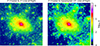 |
Fig. A.1. Convergence maps in log-scale of a cluster at z = 0.211 with M200 = 3.32 × 10¹⁴ M⊙, including LoS structure up to z = 0.25. Left: Both cluster and LoS structure mapped at 2 arcsecond resolution with the particle light-cone data. Right: Shell of the cluster from the particle lightcone data, with the other shells from the HEALPix maps upsampled from 13 to 2 arcsecond resolution. In the outskirts of the cluster, we observe that up-sampling smooths the LoS structure. |
Appendix B: Median bias in mass, concentration, and axis ratio
We have shown that LoS structure induces a positive skew in the relative error distribution. Given this skew, showing the mean bias in our free parameters is the most representative of the effects coming from LoS structure. However, in some cases, the median bias can be of interest as well.
Therefore, we present our results for the median bias for the free parameters of the sphNFW and eNFW4 models in Figures B.1 and B.2, respectively. The median is less sensitive to skewness than the mean. Consequently, the impact of LoS structure on the median mass and concentration biases is less pronounced than on the mean bias.
All Tables
All Figures
|
Fig. 1. High resolution convergence maps overlaid with reduced shear maps of an example cluster at z = 0.231 with M200 = 9.9 × 10¹⁴ M⊙. We show different lensing maps from left to right for source plane redshifts of zs = 0.8, 1.2, 2.0 and 3.0. For legibility, the reduced shear map has been down-sampled by a factor 30. At higher source redshifts, the gravitational lensing efficiency increases, but so does the amount of LoS structure. |
| In the text | |
|
Fig. 2. Two subsamples resulting from the subdivision of the main sample, based on their having an over-dense (red) or under-dense (blue) LoS for a given source redshift (shaded colours). Left: Median azimuthally averaged reduced tangential shear contribution from the LoS, calculated as the difference between the reduced tangential shear from the CL+LoS mock and the CL mock, as a function of radius. Right: Median azimuthally averaged residuals, calculated as the difference between the reduced tangential shear from the best-fit model and the CL mock. On average, the residuals for clusters lying along over-dense and under-dense sight-lines are asymmetrically distributed around zero, potentially leading to a bias. |
| In the text | |
|
Fig. 3. Applying the sphNFW model we show the mean bias (top row) and scatter (bottom row) as a function of source redshift for the cluster’s mass (left column) and concentration (right column), for our four mocks CL (black-dotted), CL+LoS (green-dashed), CL+σϵ (blue-dot-dashed) and CL+LoS+σϵ (red-solid). We estimate the bias of quantity ‘𝒬’ as the mean of the relative error distribution minus 1. We estimate the upper bound scatter (+) and lower bound scatter (−) using the 84th and 16th percentile of the relative error distribution, respectively. |
| In the text | |
|
Fig. 4. Same as Figure 3, but employing the eNFW4 model, which treats the axis ratio (q) as a free parameter (right column). |
| In the text | |
|
Fig. 5. Relative error distributions for the best-fit parameters in the Euclid+CL (purple) and Euclid+CL+LoS (orange) mocks. We show the relative error distribution for mass (left panel); concentration (right panel: top-left) under the assumption of the sphNFW model; and mass (right panel: bottom-left); concentration (right panel: top-right); and axis ratio (right panel: bottom-right) under the assumption of the eNFW4 model. We report the difference of the means (Δμ) and it’s bootstrapped uncertainty on the top right of each panel. For Euclid-like data, LoS structure positively biases mass estimates with the sphNFW model on the level of +5.3 ± 1.4%, which is significant at 3.5σ. |
| In the text | |
|
Fig. 6. Comparison of the estimated uncertainty (Nautilus, diagonal covariance matrix) and true scatter (84th percentile relative error distribution). The top panels show the results for the free parameters of the sphNFW model, while the bottom panels show the same for the eNFW4 model. For the CL+LoS+σϵ mock, the estimated uncertainty and true scatter are shown as red-dashed and red-solid lines, respectively. For the Euclid+CL+LoS mock, the estimated uncertainty and true scatter are shown in orange stars and crosses, respectively. A gray-dotted curve indicates a quantity inversely proportional to the lensing efficiency. Under the assumption of a diagonal covariance matrix, LoS-induced scatter in mass estimates is not accounted for in the Bayesian parameter inference. |
| In the text | |
|
Fig. 7. Median offset between the centre of the gravitational potential and the BCG (BCG wobble) as a function of source redshift for: the CL (black-dotted), CL+LoS (green-dashed), CL+σϵ (blue-dot-dashed), CL+LoS+σϵ (red-solid), Euclid+CL (purple-cross) and Euclid+CL+LoS (orange-cross) mocks. The error bars indicate the 1σ bootstrapped uncertainty. The red dashed line indicates the median wobble as expected from random sampling the posterior distribution for the centre on the CL+LoS+σϵ mock. For upcoming Euclid data, measured median offsets of ∼14 kpc are expected for cold dark matter, with no significant contribution of LoS structure. |
| In the text | |
|
Fig. A.1. Convergence maps in log-scale of a cluster at z = 0.211 with M200 = 3.32 × 10¹⁴ M⊙, including LoS structure up to z = 0.25. Left: Both cluster and LoS structure mapped at 2 arcsecond resolution with the particle light-cone data. Right: Shell of the cluster from the particle lightcone data, with the other shells from the HEALPix maps upsampled from 13 to 2 arcsecond resolution. In the outskirts of the cluster, we observe that up-sampling smooths the LoS structure. |
| In the text | |
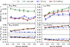 |
Fig. B.1. Same as Figure 3, but now with the median bias instead of the mean. |
| In the text | |
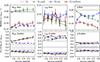 |
Fig. B.2. Same as Figure 4, but now with the median bias instead of the mean. |
| In the text | |
Current usage metrics show cumulative count of Article Views (full-text article views including HTML views, PDF and ePub downloads, according to the available data) and Abstracts Views on Vision4Press platform.
Data correspond to usage on the plateform after 2015. The current usage metrics is available 48-96 hours after online publication and is updated daily on week days.
Initial download of the metrics may take a while.