| Issue |
A&A
Volume 703, November 2025
|
|
|---|---|---|
| Article Number | A186 | |
| Number of page(s) | 16 | |
| Section | Interstellar and circumstellar matter | |
| DOI | https://doi.org/10.1051/0004-6361/202555449 | |
| Published online | 17 November 2025 | |
Millimetre continuum from luminous blue variable stars and their environs
NIKA2 observations and Virtual Observatory data★
1
ISDEFE,
Beatriz de Bobadilla 3,
28040
Madrid,
Spain
2
INAF – Osservatorio Astrofisico di Catania,
Via Santa Sofia 78,
95123
Catania,
Italy
3
Université Grenoble Alpes, CNRS, LPSC-IN2P3,
53, avenue des Martyrs,
38000
Grenoble,
France
★★ Corresponding author: This email address is being protected from spambots. You need JavaScript enabled to view it.
Received:
8
May
2025
Accepted:
27
August
2025
Abstract
Context. Luminous blue variables (LBVs) represent a brief transitional phase in the evolution of massive stars. Multi-wavelength studies of their circumstellar environments are essential to quantify their feedback at Galactic scales. Dominant emission mechanisms at millimetre wavelengths are, however, still poorly understood.
Aims. Stellar winds, circumstellar dust, and ionised gas have not been explored together in the case of LBVs. We aim to study the millimetre continuum emission of Galactic LBVs to disclose the presence of these components, to describe their morphology, and to measure their relevance in the mass and energy injection to the interstellar medium.
Methods. We used the NIKA2 continuum camera at the IRAM 30 m radio telescope to observe and analyse 1.15 and 2 mm continuum from the LBVs HD 168607, HD 168625, [GKF2010]MN87, [GKF2010]MN101, and G79.29+0.46. We used the Virtual Observatory to complement our observations with archival data from optical, infrared, millimetre, and centimetre wavelengths. With this information, we built complete spectral energy distributions (SEDs) for the five sources that cover six decades of the electromagnetic spectrum.
Results. All targets except MN87 were detected at both wavelengths, with features including compact sources, extended nebular emission, shells, and unrelated background structures. The spectral indices of compact sources are consistent with thermal emission from stellar winds. We modelled the SEDs and successfully reproduced the emission from stellar photospheres, circumstellar dust, thermal stellar winds, and enshrouding H II regions. Our models, in agreement with previous literature results, reveal unresolved hot dust very close to the stars and provide the first estimates for the fundamental parameters of MN101.
Conclusions. This pilot study highlights the great potential of millimetre continuum studies of LBVs and possibly other evolved massive stars. The millimetre spectral window bridges the far-IR and radio regimes and can disclose the relative contribution of dust and free-free emission in this type of source.
Key words: astronomical databases: miscellaneous / virtual observatory tools / circumstellar matter / stars: evolution / stars: massive / radio continuum: stars
This work is based on observations carried out under project number 044-17 with the IRAM 30m telescope. IRAM is supported by INSU/CNRS (France), MPG (Germany), and IGN (Spain).
© The Authors 2025
 Open Access article, published by EDP Sciences, under the terms of the Creative Commons Attribution License (https://creativecommons.org/licenses/by/4.0), which permits unrestricted use, distribution, and reproduction in any medium, provided the original work is properly cited.
This article is published in open access under the Subscribe to Open model. This email address is being protected from spambots. You need JavaScript enabled to view it. to support open access publication.
1 Introduction
The late evolutionary stages of high-mass stars affect the shape and evolution of the Milky Way. As these massive stars evolve through a series of transitional phases to their endpoint as core-collapse supernovae (Langer et al. 1994), their intense UV fields and conspicuous mass-loss deeply transform the dynamics, structure, and chemical composition of their environs. Among these stages, a short interlude of ~104 yr known as the luminous blue variable phase (hereafter LBV) stands out as a main contributor in terms of its radiative and mechanical output (Humphreys & Davidson 1994) through high mass-loss rates (![Mathematical equation: $\[\dot{M}\]$](/articles/aa/full_html/2025/11/aa55449-25/aa55449-25-eq1.png) up to 10−4 M⊙ yr−1) and occasional eruptions (shedding up to some ~10 M⊙ on extremely short timescales). These episodes of enhanced mass loss that may rival the energetic output of supernovae (Smith 2013) leave an indelible footprint in the outskirts of these stars and give rise to complex and heterogeneous circumstellar nebulae of dust and gas (Weis 2001, 2011).
up to 10−4 M⊙ yr−1) and occasional eruptions (shedding up to some ~10 M⊙ on extremely short timescales). These episodes of enhanced mass loss that may rival the energetic output of supernovae (Smith 2013) leave an indelible footprint in the outskirts of these stars and give rise to complex and heterogeneous circumstellar nebulae of dust and gas (Weis 2001, 2011).
This circumstellar material has been probed by diverse observational strategies. Infrared continuum and spectroscopy revealed the existence of different circumstellar dust populations around some stars, traced by successive mass-loss events (Jiménez-Esteban et al. 2010; Vamvatira-Nakou et al. 2013, 2015; Buemi et al. 2017), and yielded valuable insights into the chemistry and dust lifecycle around these sources (Gull et al. 2020). Continuum emission at centimetre wavelengths traced the distribution of ionised gas around the stars and detected their thermal stellar winds, which enabled accurate estimates of their mass-loss budget (Duncan & White 2002; Umana et al. 2010; Ingallinera et al. 2016) and, under some assumptions, their present-day mass-loss rate (Umana et al. 2005, 2012). Molecular spectroscopy studies of the millimetre window revealed molecular structures that trace swept-up material and previous events of mass ejection. This component is critical to our understanding of the physical processes that drive the evolution of the circumstellar material (i.e. energy and mass-loss balance) (Rizzo et al. 2008; Bordiu et al. 2019, 2021) and its chemical complexity (Rizzo et al. 2014; Morris et al. 2020; Bordiu et al. 2022; Rizzo et al. 2023).
The millimetre region of the electromagnetic spectrum is, a priori, the region in which cold dust and ionised gas can contribute significantly through continuum emission. Observations in this range are therefore needed to characterise and constrain the relative importance of each component. Despite its potential relevance, there has been limited research on the (sub) millimetre continuum emission of LBV stars. In the Galaxy, we only found observational studies of G79.29+0.46 (Higgs et al. 1994), Wd1-243 (Fenech et al. 2018), η Car (Bordiu et al. 2019), and AG Car (Bordiu et al. 2021). In the first two cases, there are only flux measurements at the central source, while in AG Car, it was detected the central source and weak emission from the surrounding nebula. In η Car, the millimetre continuum maps revealed the stellar wind and the extended ejecta from the 1890 outburst.
A handful of extragalactic LBV stars in the Large Magellanic Cloud have also been observed: S61, RMC 127, and RMC 143 (Agliozzo et al. 2017a,b, 2019, respectively), and all of them are known to harbour dense circumstellar nebulae that are visible at infrared or centimetre wavelengths. In the case of S61, neither the central star nor the shell were detected; RMC 127 appeared as a point-like source, but the nebula was not detected; and RMC 143 was clearly detected, surrounded by a massive resolved nebula of dust and ionised gas, different in morphology from the circumstellar material observed at longer wavelengths.
The disparity of results in such a small source sample underlines the relevance of the (sub) millimetre characterisation as a valuable tool in the study of these objects. The millimetre regime is the range in which thermal dust and bremsstrahlung emission compete, so that observations in this band are fundamental for separating their contribution to the overall mass-loss budget.
To mitigate this lack of sampling and gain a better understanding of the processes governing emission in this part of the spectrum, we used the NIKA2 continuum camera at the IRAM 30 m telescope and carried out a pilot study of the 1 and 2 mm continuum emission of five Galactic LBV stars (see Table 1). We list the sources below.
HD 168607. Located at a distance of ~1.8 kpc (Gaia Collaboration 2022), this source is a confirmed LBV star of spectral type B9Ia+ (Clark et al. 2012) that shows no signs of circumstellar material (Hutsemekers et al. 1994).
HD 168625. Projected in the sky at ~1 arcmin and slightly closer to HD 168607, this star is a supergiant of spectral type B8Ia+ (Clark et al. 2012). It is enshrouded in an hourglass-shaped nebula that was likely produced by binary interaction (Martayan et al. 2016; Mahy et al. 2016). It is also recognised as a nearly perfect analogue of the circumstellar environment of SN1987A (Smith 2007). Because substantial variability is not fully demonstrated (Clark et al. 2012), it remains a candidate LBV. It is one of the less luminous stars of its type (Smith et al. 2004).
[GKF2010]MN87 (hereafter MN87). This source was first discovered through its associated bright and asymmetric shell with a radius of 28 arcsec in the MIPSGAL survey (Mizuno et al. 2010). It was promptly identified as as a massive star based on infrared spectroscopy (Wachter et al. 2010; Gvaramadze et al. 2010). It was later proposed to be a LBV candidate on the basis of high-resolution radio observations (Ingallinera et al. 2014, 2016). The central source of the nebula is compatible with a thermal stellar wind and a clumpy ionised shell. Its distance is unknown. At an assumed radius of 0.3–0.6 pc that is typical of other LBV shells, the most likely range of distances is 2–4 kpc.
[GKF2010]MN101 (hereafter MN101). This source was also discovered in MIPSGAL as a nebula with a diameter of ~20 arcsec and was proposed to be a LBV candidate by NIR spectroscopy of the central source (Wachter et al. 2011; Flagey et al. 2014). Ingallinera et al. (2014, 2016) studied its radio emission and revealed a central source with a canonical thermal wind and an ionised nebula co-spatial with the infrared, characterised by a negative spectral index. Finally, Bordiu et al. (2019) detected a CO torus that is wrapped around the infrared nebula, with a low [12CO/13CO] ratio that is indicative of CNO-processed material. The distance to this source is uncertain; the most likely range of geometric distances estimated from Gaia parallaxes (Bailer-Jones et al. 2021) is 3.0–6.2 kpc.
G79.29+0.46. This source is an archetypal LBV candidate (Waters et al. 1996) surrounded by a series of nested infrared shells (Voors et al. 2000; Jiménez-Esteban et al. 2010) associated with successive mass-loss episodes. The innermost shell has an ionised counterpart detected in radio-continuum observations (Umana et al. 2011; Agliozzo et al. 2014), and a molecular counterpart traced by CO emission (Rizzo et al. 2008) that partially interacts with the nearby infrared dark cloud (IRDC) G79.3+0.3 (Palau et al. 2014). Some warm hotspots of ammonia have also been reported in and within the shell (Rizzo et al. 2014). The distance to G79.29+0.46 is 1.75 kpc (Gaia Collaboration 2022).
The continuum maps delivered by the NIKA2 camera have fields of view (FOV) of several arcminutes, enabling the simultaneous study of the stars and their surroundings, with the potential to reveal multiple co-existing emission mechanisms. In Sect. 2, we describe the observations. In Sect. 3 we present the main results, including the overall maps, zoom-ins around the stars, and a study of the millimetre spectral indices. In Sect. 4, we complement the information by constructing spectral energy distribution (SED) diagrams from the optical to radio wavelengths. In Sect. 5, we identify and model the components in the SEDs, which allowed us to draw some general ideas about the dominant emission mechanisms. We conclude with a general discussion of the survey and the individual sources in Sect. 6.
Observed sources.
2 Observations
The observations were made with the NIKA2 continuum camera (Perotto et al. 2020) available at the IRAM 30 m radio telescope during three consecutive runs in October 2017 (project 044-17; PI R. Rizzo). The weather was stable during all the sessions, with measured opacities at 225 GHz between 0.2 and 0.3, which is equivalent to a precipitable water vapour between 3 and 5 mm.
For the four regions of interest, we performed a total of 126 individual on-the-fly maps with a duration of three to five minutes each. The scanning angles were 0,45, and 90 degrees to avoid stripping effects in the reconstruction of the final maps. An additional 15% were added in size to the definition of the maps to account for a better reconstruction of the background noise. The pointing was regularly checked, with corrections always below 4 arcsec. The FOV for all sources but G79.29+0.46 was 6.5 arcmin. In G79.29+0.46, we observed with 8.6 arcmin of FOV in order to include the previously known infrared shells and the nearby IRDC.
The NIKA2 camera has three arrays (two at 260 GHz and one at 150 GHz) filled with thousands of kinetic inductance detectors (KIDs) that provide an accurate combination of the responses from off-source detectors to reconstruct the noise template that is to be subtracted from the data. To produce the final images, we used a data-analysis pipeline based on MOPSIC (Zylka 2013) and developed by the NIKA2 collaboration prior to the first public release of PIIC1. In order to preserve large-scale features, we used an iterative procedure. In the first iteration, the software accounted for the absolute calibration of the flux and the opacity correction and merged all collected maps. As output of this first iteration, we had a first attempt of the total map. This was used to estimate the S/N on the map and extrapolate the region with maximum brightness. The extrapolated structure of the source was used as a mask that was introduced in a second round of iteration. At the end of this latter, we obtained a convergence map that resulted from the difference between the two previous maps. When the brightness of the convergence map exceeded a well-defined threshold in the central region, the process continued and a third iteration started. This method is based on minimising the residuals on the final map and allowed us to recover the largest scales in case of extended emission.
The rms map values of the four fields are depicted in Fig. 1. The values were computed as averages over concentric rings with a width of 2 arcsec. At 1.15 mm (260 GHz), the noise map is rather uniform up to 120–140 arcsec of the centre, while at 2 mm (150 GHz), it extends well beyond 200 arcsec.
Finally, we smoothed the maps with a Hanning 3 × 3 kernel to improve the S/N. The resulting angular resolution (half-power beam width; HPBW) after this step was 12.5 and 18.5 arcsec at 1.15 and 2 mm, respectively. With the smoothing, the rms was reduced by a factor of about 0.36 in all cases.
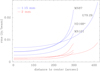 |
Fig. 1 Noise map of the observed fields. The rms noise was computed in concentric rings with a width of 2 arcsec. The noise in the 1.15 mm maps is plotted in blue, and the noise corresponding to the 2 mm maps is plotted in red. The field names (abridged) are indicated near the 1 mm curves. |
3 NIKA2 results
3.1 Emission from the stars and their surroundings
The final processed maps are presented in Fig. 2. Overall, we note emission from the stars, circumstellar structures, and other likely unrelated features. A close-up of the emission at the positions of the stars is depicted in Fig. 3, and the zoom at 1.15 mm and 2 mm is depicted in the top and bottom rows, respectively. To facilitate a visual inspection of the point-like nature of the sources, we highlight a contour corresponding to 50% of the continuum peak, together with the HPBW at each frequency.
HD 168625 and HD 168607 are detected in both bands, but more clearly at 2 mm. The entire field is relatively devoid of significant emission, except around the stars. In the case of HD 168625, the source appears to be slightly resolved. At 1.15 mm, it shows a faint extended emission plateau that peaks towards the south-west and might be linked to the complex hourglass-shaped nebula that enshrouds the star at infrared wavelengths (Smith 2007). At 2 mm, however, the emission is rather circular, and the maximum agrees well positionally with the star. On the other hand, HD 168607, which lacks reported circumstellar material, is unresolved at 2 mm and very probably also at 1.15 mm, although the low S/N prevents a more detailed analysis.
MN87 is not detected in either band. The field is dominated by a series of filaments that are brighter at 1.15 mm. These structures are well correlated with the dust bands seen in the images at 250 and 500 μm from Herschel/SPIRE (Molinari et al. 2010).
The field of MN101 is dominated by a bright emission region towards the north that likely corresponds to a molecular cloud that is not related to the star. Towards the centre of the map, two components are barely resolved: A central compact emission that matches the position and size of the infrared nebula, possibly embedded in a plateau, and a more diffuse component located about 30 arcsec to the south-east, corresponding to the brightest region of the CO structure reported by Bordiu et al. (2019). While the brightness of the two components is similar at 1.15 mm, the central source dominates at 2 mm.
In the field of G79.29+0.46, the bright IRDC stands out. It extends from the south-east to the west. The central source is well detected in the two bands, with notably brighter emission at 2 mm. A shell-like structure surrounding the star from the north-east is also detected faintly at 1 mm and clearly at 2 mm. This structure has an approximate radius of 100 arcsec, which means that it is most likely associated with the innermost infrared dust shell, as is visible in Spitzer images (Jiménez-Esteban et al. 2010). This millimetre shell is bounded by the CO shells reported by Rizzo et al. (2008).
Table 2 lists the flux densities of the central sources at 1.15 and 2 mm along with their associated uncertainties, centroids, and sizes. They were all derived from Gaussian fitting. The last column also shows the spectral indices, which are discussed in the next section.
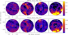 |
Fig. 2 Sky maps of the millimetre continuum emission in the four fields observed with NIKA2. The maps at 1.15 mm are shown at the top row, and the 2 mm maps are shown at the bottom. The field that contains HD 168607 and HD 168625, labelled HD168*, is centred on HD 168625. The colour scales (indicated at the right of each row) are in Jy beam−1. HPBWs are drawn near the bottom left corners of the HD168* images. The central areas indicate the zoomed region displayed in Fig. 3. |
3.2 Millimetre spectral indices
We computed the spectral indices of the central sources between the two NIKA2 frequencies (αmm hereafter) following the convention Sν ∝ να. Despite the low S/N at 1 mm, it is evident overall that all the detected sources except MN101 exhibit values close to a thermal stellar wind (αmm ~ 0.6), which is indeed expected for the strong winds driven by LBV stars.
On the other hand, we built the maps of αmm for all the observed fields after convolving them to a common beam of 20 arcsec. We only used pixels with brightness above a 2σ threshold in the convolved maps. The resulting maps are shown in Fig. 4. They reveal a diverse range of features that are likely due to multiple emission mechanisms.
HD 168625 shows a somewhat negative index, consistent with an ionised H II region. As a consequence of the convolution, the emission at 1 mm is severely diluted and at the centre displays the contribution of the central source plus that of an additional component, which is probably close-in young stellar ejecta. In contrast, HD 168607 displays slightly positive values of αmm that are more compatible with a thermal stellar wind. This is in line with the values reported in Table 2.
In the case of MN87, the dominant emission arises primarily from filaments that cross the whole field. These features have high values of αmm, which is typical of thermal dust emission. Considering their morphology as well, we suggest that the millimetre emission in this field very likely arises from foreground or background Galactic clouds.
MN101 presents a more complex scenario in which the central region depicts negative values of αmm. Again, the NIKA2 beam plays a critical role: The size of the infrared nebula is comparable to the beam, so that the negative spectral index likely captures the combined contribution of the stellar wind and the nebular material, which is known to show non-thermal emission in the centimetre regime (Ingallinera et al. 2016). The nebula is embedded in a free-free plateau and is surrounded by thermal dust (in yellow). This agrees well with well-known molecular structures (Bordiu et al. 2019). The highest spectral indices in this enshrouding structure are located south-west of the star, in coincidence with the brightest part of the CO cloud.
G79.29+0.46 is perhaps the most puzzling object. The central region exhibits a rather negative αmm, in contrast with the positive value derived for the central source in Table 2 (i.e. not convolved). While the fitted value agrees relatively well with the α = 0.6 derived by Higgs et al. (1994) at 0.8, 1, and 1.2 mm, the negative value observed in the map is a consequence of the severe dilution of the 1 mm central point source (around 0.39).
G79.29+0.46 is known to host a set of concentric shells at angular distances of 100–200 arcsec from the exciting star (Rizzo et al. 2008; Jiménez-Esteban et al. 2010; Agliozzo et al. 2014). The inner shell is clearly visible in Fig. 4, where it shows a remarkable stratification at its eastern side around position (100″, −20″), with three distinct components. Farther away, there is a transition from negative values, which might indicate shocked material, to flat values corresponding to the ionised shell, and finally, to positive values associated with the thermal dust surrounding the shell. A secondary, less pronounced stratification is evident in the south-west region, where the shell interacts with a nearby IRDC (Rizzo et al. 2008; Palau et al. 2014), and where we measure the highest values of αmm (red in Fig. 4).
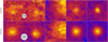 |
Fig. 3 Zoomed sky maps around the central sources. The regions correspond to the regions indicated in Fig. 2. To span the full dynamic range, the colour scale is different for each of the maps. The contours correspond to 30, 50 (highlighted in white), and 70% of the maximum value. HPBWs are indicated near the bottom of the HD168* images. The contours at 50% are highlighted to facilitate a visual comparison with the beam and give an idea about the point-like nature of the central sources. |
Two-dimensional Gaussian fitting.
4 SED analysis
4.1 Building
Aiming to study the relative contribution of the different physical processes that dominate the emission of our targets, we constructed their SEDs along virtually the whole electromagnetic spectrum. We were interested in the study of the circumstellar gas and dust and therefore focused the analysis on the infrared, millimetre, and radio domains.
For each target star, we proceeded in a number of sequential steps that we describe below.
We constructed a Python script to retrieve all the photometry data available in VizieR. The script was validated after comparing its outputs with the VizieR photometry tool2. The structure of the script outputs is similar to that of VizieR, with the addition of the wavelength in microns.
We initially ran the script with a search radius of 3 arcsec.
In order to check possible data that were lost beyond 3 arcsec (typically, in the infrared to centimetre wavelengths), we performed a second search by changing the search radius to 30 arcsec.
We removed duplicated information, which gave more priority to original data and to data that included flux uncertainties, instead of compiling other surveys and data without quoted uncertainties.
In the VizieR database3, we checked all the literature information about the targets. This step was performed to incorporate possible data from catalogues that were not included in the photometry tool.
We used the Simbad service4 to check and incorporate data from observational papers that were not included in the VizieR database.
Table A.1 (in Appendix A.1) lists all the datasets we used to build the SEDs. In addition to the catalogue names, the VizieR table number, the wavelength range, and the bibliographic reference are included. The Appendix A.2 enumerates a series of additional information about each of the stars that we noted in our tailored search for multi-wavelength photometry.
 |
Fig. 4 Spectral index maps between the two NIKA2 frequencies. The plotted field and marks are the same as in Fig. 2. For each map, all pixels with brightness below 2σ were masked. |
4.2 Clarification on particular datasets
Gaia. With the Gaia DR3 photometry data, we additionally checked the consistency of the G-band flux with respect to the BP and RP fluxes. This effect is a consequence of different background estimates for the G and the BP and RP bands5. While the G flux is determined by fitting a profile function, the BP and RP fluxes are determined by aperture photometry. The different approach may be critical in our case, where the targets are often very red due to surrounding warm dust and, at the same time, affected by contamination of other (bluer) stars due to their low Galactic latitude. The consistency is measured by the so-called excess factor, defined as the sum of fluxes in the BP and RP bands, divided by the flux in the G band; this factor is slightly above one in most cases. However, we noted very high excess factors in all the sources (1.41, 1.38, 2.14, 2.17, and 1.83 for the sources ordered as in Table 1). This fact might be interpreted by an incorrect measurement of the background in G (due to the inclusion of nebular material), rather than by contamination in BP and RP bands. In consequence, we did not consider the G-band fluxes for the SED fitting.
GLIMPSE. Its photometry is potentially affected by extended nebular emission, mainly due to the additional contribution of line emission and PAHs. A priori, this contamination may affect MN101, MN87, and HD 168625, which are the sources in which the nebular material is not completely detached from the star. Upon inspection of the fluxes, we confirm that MN87 and MN101 are not affected, as their nebular emission is only detected at 24 μm (Mizuno et al. 2010). In contrast, in HD 168625, the VizieR photometry tool only reports flux at 5.8 μm, while the catalogue itself gives data at 3.6, 4.5, and 5.8 μm (all of them are well below the fluxes from other catalogues, however). Consequently, we removed these data points from the HD 168625 SED.
Radio. The radio data we used to build the SEDs come from targeted high-resolution observations and all-sky surveys conducted at various radio facilities. Consequently, the angular resolution can vary by up to a factor of ~10. While the highest-resolution data points measure the flux of the central stellar source directly, the lowest-resolution data points may include emission from the star and the circumstellar material, except when the star is completely detached from the nebula. When we were unable to separate the two components, the data points contained the sum of the flux densities corresponding to the stellar wind and the surrounding nebula (modelled as bremsstrahlung, as explained in Sect. 5.1).
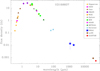 |
Fig. 5 Spectral energy distribution of HD 168607 in logarithmic scale. The catalogues are indicated at the top right. The corresponding error bars of all points are plotted. The NIKA2 points are shown with blue stars. |
4.3 Resulting SEDs
The resulting SEDs are depicted in Figs. 5–9. All of them are highly reddened, as their visual or near-IR peaks are in the range from 1 to 3 μm. This behaviour is indeed expected, considering the long distances of the stars, their location in the Galactic plane, and their nature as dust producers.
Roughly, we distinguish two types of SEDs. The first type is represented by HD 168607 (Fig. 5) and G79.29+0.46 (Fig. 9), where the fluxes decrease monotonically from IR to millimetre to centimetre wavelengths. In both cases, the NIKA2 fluxes are significantly higher than the radio fluxes (up to one order of magnitude). No resolved ejecta structures fall within the NIKA2 beam in the two sources (see Fig. 3), so that the measured flux is most likely the combined contribution of the stellar wind and close-in unresolved dust.
The second type of SEDs is that of HD 168625 (Fig. 6) and MN101 (Fig. 8). The two sources are immersed in conspicuous gaseous and dusty nebulae that contribute to the emission observed with NIKA2. Both SEDs are rather flat in the millimetre-centimetre range, with NIKA2 fluxes comparable to centimetre wavelength fluxes (slightly below in HD 168625 and slightly above in MN101), of the order of 10 mJy. In the infrared, both stars show a strong bump that peaks at ~20–30 μm, which probably indicates a large amount of warm circumstellar dust.
MN87 is a puzzling object. It exhibits strong infrared emission without a well-defined peak. This behaviour is not observed in the other four sources (for which we applied the same processing) and is likely related to the different instrument apertures. In MN87, this effect seems to be a critical factor due to widespread Galactic contamination, as indicated by the dominance of SPIRE dust structures in the NIKA2 maps (see Sect. 3.1). At centimetre wavelengths, the hot star (more properly, its stellar wind) is clearly detected, with flux densities comparable to those of MN101 (Ingallinera et al. 2016).
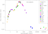 |
Fig. 6 Spectral energy distribution of HD 168625. |
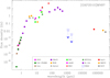 |
Fig. 7 Spectral energy distribution of [GKF2010]MN87. |
5 Multi-wavelength modelling
5.1 Fitting methodology
The environs of LBV stars are strongly affected by their strong UV radiation and powerful winds. Under adequate physical conditions, LBVs are also efficient dust producers. The continuum emission in these environments is dominated by a combination of thermal dust radiation and free-free emission produced by stellar winds and ionised nebular gas. Non-thermal emission may also be present under special circumstances, such as colliding winds in binary stars, as in HD 168625 (Martayan et al. 2016; Mahy et al. 2016), after mass ejection events, or in the presence of shocks.
The SEDs we compiled and curated in the previous sections demonstrate that our targets depict all the above components with diverse significance at different wavelength ranges. Even more, the millimetre range is key to constraining the contribution of the warm or cold dust, and at the same time, the highly ionised stellar wind. We therefore proceeded to model the observed SEDs with the aim to evaluate the relative importance of these components. The models are intended to be as simple as possible, with the minimum number of parameters capable of providing robust estimates of the different physical components. Because the SEDs always arise from a single position and lack spectroscopic information, we did not attempt to provide fine details about the space distribution and velocity field of our targets. In some cases, we assumed reasonable physical quantities after determining their influence in the flux predictions. For each modelled component, Appendix B details these aspects in depth.
The first step was to correct the stellar fluxes by interstellar extinction according to the Bayestar19 3D dust model (Green et al. 2019). We assumed the distances quoted in Table 1, adopting 3 and 4 kpc for MN87 and MN101, respectively. We used the Python package dustmaps (Green 2018), which provides extinction values for grizy and JHK bands, and interpolated the available photometry by a cubic spline. After this initial correction, we noted still significant remaining reddening in all the sources. This is indeed expected considering the presumed presence of circumstellar dust close to the extended star atmospheres. A follow-up determination of the total extinction was subsequently performed for wavelengths smaller than 4.6 μm (for details see Green et al. 2019), which allowed us to separate the interstellar and the circumstellar extinction at each optical or near-IR band. For this step, we considered effective temperatures (Teff) from 8000 to 20 000 K, which is the range corresponding to all the known LBVs (Smith et al. 2004).
We modelled the extinction-corrected SEDs as a sum of independent flux contributors. We included four types of components: (1) a central star, modelled as a black body; (2) one or more circumstellar dust clouds, conceived as black or grey bodies at different temperatures; (3) stellar wind, modelled as a homogeneous and isotropic mass loss at a constant rate; and (4) free-free emission arising from a homogeneous ionised nebula surrounding the hot star. Appendix B describes all these components in detail, including the free parameters and assumptions involved.
It is challenging to model a SED from the optical to the radio bands (i.e. more than six decades). The spectral regions have diverse coverage, aperture, and sampling; and all the flux measurements are also potentially affected by intrinsic variability of the sources, geometry, and composition, among other factors.
We followed an iterative fitting procedure to ensure that each component was constrained progressively. First, we divided each SED into four spectral regions, bounded by the wavelengths in which the contribution of two components was comparable. In general terms, the four regions are (1) optical to a few microns, dominated by the contribution of the stellar photosphere; (2) near-infrared up to some tens of microns, with contributions mainly from the star and a hot dust component; (3) mid-infrared up to the NIKA2 points, dominated by warm- or cold-dust components and free-free emission; and (4) millimetre and centimetre wavelengths, mostly dominated by ionised gas and/or the stellar wind. We adopted a stepwise approach, starting from the optical region and progressively incorporating additional components, as described below.
We started by fitting the optical part of the SED by the stellar photosphere alone. The parameter space representative of LBV stars (Teff from 8000 to 20 000 K and stellar radius Rstar from 30 to 300 R⊙) was employed as a kick-off exploration and was later refined through χ2 minimisation.
Then, we proceeded to fit the near-infrared region. The star component was combined with an additional greybody representing a hot-dust component. The stellar parameters were kept within a narrow range around the previously determined parameters, while the dust parameters were probed in wide ranges (Rdust from 0.5 to 20 au, (Tdust from 500 to 3000 K, and β from 0 to 2). We repeated the χ2 minimisation to locate the new best-fit parameters for the star and the hot-dust components.
As a next step, we refined the fit over the two previous ranges to ensure consistency between the two components and further constraining the parameter space around previously found minima, thus obtaining a new set of best-fitting parameters.
The above steps were repeated by iteratively incorporating the remaining components at the other wavelength ranges, until the whole SED was fitted and the best-fit parameters for all the components were determined.
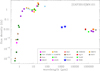 |
Fig. 8 Spectral energy distribution of [GKF2010]MN101. |
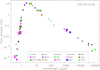 |
Fig. 9 Spectral energy distribution of G79.29+0.46. |
Best-fit model results.
5.2 Fitting results
The NIKA2 upper limits of MN87 are not sufficient to constrain all the SED components and keep a physical meaning. On one hand, the strong infrared emission of this source requires a very high emissivity index (β ≫ 2) to obtain the necessary drop at NIKA2 frequencies. On the other hand, the ~10 mJy level of the radio emission requires a deeply negative value of α. In order to find some explanation, both parts of the spectrum must be taken into account; it is known that non-thermal processes are important in this source (Ingallinera et al. 2016), and the mid-infrared SED points may be heavily contaminated by background emission.
For the other stars, Table 3 summarises the best-fit results. It includes the fundamental stellar parameters (Teff and radius Rstar), the interstellar and circumstellar absorption in g band, the parameters of the dust components (dust temperature Tdust, the characteristic radius Rdust, and the total dust mass Mdust) and, depending on the case, the current mass-loss rate ![Mathematical equation: $\[\dot{M}\]$](/articles/aa/full_html/2025/11/aa55449-25/aa55449-25-eq5.png) of the stellar wind, or the parameters of the free-free model (electron density ne and size of the ionised region Rff). Furthermore, Fig. 10 displays the four best-fit models, together with the individual components and the de-reddened photometry. The four SEDs are plotted at the same scale to facilitate visual comparison.
of the stellar wind, or the parameters of the free-free model (electron density ne and size of the ionised region Rff). Furthermore, Fig. 10 displays the four best-fit models, together with the individual components and the de-reddened photometry. The four SEDs are plotted at the same scale to facilitate visual comparison.
It is noteworthy that the two stars with the highest Teff, HD 168607 and G79.29+0.46, are also the two whose SEDs were fitted by including a stellar wind component. In contrast, HD 168625 and MN101 were fitted by the low-end of the usual values of Teff, and both were fitted by free-free components. The circumstellar extinction is high in all cases, being HD 168607 the less reddened of the sample. The warm- or cold-dust masses are remarkably similar, of the order of 10−3 M⊙. The hot dust masses, however, are three orders of magnitude lower, except for the much higher Mdust of HD 168625, which is in line with the huge IR emission from its dust nebula. The mass-loss rates inferred from the stellar winds of HD 168607 and G79.29+0.46 are of the order of a few 10−6 M⊙ yr−1 (scaled to v∞ = 100 km s−1; see Appendix B for details).
In the four cases, the relevance of the NIKA2 data is evident. At 1–2 mm, it is clearly noted that the observed flux results as the combined contribution from the ionised stellar wind (or ionised nebula) and the cold dust. The NIKA2 fluxes are vital to constrain the relative contribution of the two components arising from the far-infrared and from centimetre wavelengths.
Below, we compare our fitting results with those available in the literature.
HD 168607. The best-fitting model predicts an effective temperature of 17 000 K, which is higher than the value of ~104 K determined by Clark et al. (2012). The luminosity resulting from our fitting is 105.88±0.19 L⊙, which agrees well with the estimates provided in the same work, and inferred from a visual inspection to one of its figures. A hot-dust component lies very close to the star (Tdust = 1100 K) and causes most of the emission in the near-infrared, and a more extended but still unresolved cold-dust component (35 K) that causes the bump observed around 100μm. The radio part of the SED is well fitted by a stellar wind. Leitherer et al. (1995), based on 8.64 GHz continuum, determined ![Mathematical equation: $\[\dot{M}\]$](/articles/aa/full_html/2025/11/aa55449-25/aa55449-25-eq6.png) = 2.3 ± 0.5 × 10⁻⁶ M⊙ yr−1, using 2.2 kpc and 140 km s−1 for the distance and for v∞, respectively. Their value of M corrected for the distance of 1.84 kpc shifts to 1.5 ± 0.3 × 10⁻⁶ M⊙ yr−1. On the other hand, when we correct our
= 2.3 ± 0.5 × 10⁻⁶ M⊙ yr−1, using 2.2 kpc and 140 km s−1 for the distance and for v∞, respectively. Their value of M corrected for the distance of 1.84 kpc shifts to 1.5 ± 0.3 × 10⁻⁶ M⊙ yr−1. On the other hand, when we correct our ![Mathematical equation: $\[\dot{M}\]$](/articles/aa/full_html/2025/11/aa55449-25/aa55449-25-eq7.png) considering v∞ = 140 km s−1, we obtain 1.4 ± 0.4 × 10⁻⁶ M⊙ yr−1, which agrees perfectly with Leitherer et al. (1995).
considering v∞ = 140 km s−1, we obtain 1.4 ± 0.4 × 10⁻⁶ M⊙ yr−1, which agrees perfectly with Leitherer et al. (1995).
HD 168625. According to Table 3, the luminosity derived from our model is 104.93±0.27 L⊙. The strong infrared emission was fitted by a combination of a blackbody and a greybodies. The blackbody corresponds to a compact dust component of Tdust = 500 K (below the 1000–2000 K of the other targets by far), while the greybody represents a more extended warm-dust component (Tdust = 140 K). This is the only source in which a greybody component was required to fit the data because it was the only way to reconcile the far-infrared emission with the NIKA2 millimetre measurements.
The best-fit emissivity index, β = 1.0 ± 0.2, indicates the dust to some extent. Theoretical models (Draine & Lee 1984) predict β values between 1 and 2, with the higher values in the diffuse ISM (Planck Collaboration 2014) and the lower values in dense cores (Forbrich et al. 2014) and circumstellar disks (Friesen et al. 2018). Physical conditions in the outskirts of evolved massive stars differ markedly from those in the ISM, which are characterised by diffuse radiation fields, low temperatures, and low densities. The close environs of these hot stars are bathed by strong UV radiation fields, but at the same time, self-shielding is possible due to the continuous mass injection through the dense stellar winds.
Therefore, the value of β derived from the fitting is indicative of large grains that formed through continuous accretion, favoured by the current photospheric temperature. Kochanek (2011) proposed that episodes of enhanced mass loss might be produced during the cold phase of LBV stars and create appropriate conditions (in terms of density and self-shielding) for the grain growth. This scenario is further supported by the study of the dust around the LBV HR Car, performed by Buemi et al. (2017), which revealed a radial gradient in β, with lower values near the star and an increase at larger distances, where smaller grains mix with the ISM.
In order to proceed to a fair comparison of our estimates with other published parameters, it must be considered that the assumed distance to HD 168625 may significantly differ from one paper to the next, with obvious systematic deviations of the quoted values. We therefore re-scaled the published parameters to 1.53 kpc (Table 1) when necessary.
O’Hara et al. (2003) imaged the nebula at several near- and mid-IR wavelengths, assuming a distance of 2.8 kpc. After scaling their distance to ours, their fundamental stellar parameters closely agree with our estimates: Teff = 14 000 K and Rstar = 82 M⊙. They also obtained a dust mass of ~7.5 × 10⁻⁴ M⊙, again after correcting to our distance. This is somewhat lower than the values shown in Table 3, but still within the uncertainties. Even so, the difference may indicate a real value of κ0 that is slightly higher than we assumed in this work, probably closer to 0.9 cm2 g−1.
The stellar luminosity computed by us is substantially lower than that of Mahy et al. (2016), which is 105.58±0.11 L⊙ also assuming a distance of 2.8 kpc. This difference cannot be explained in terms of uncertainties. After correcting their value to a distance of 1.53 kpc, however, we obtained ~105.05 L⊙, which is fully compatible with our luminosity estimates. In the next section, we discuss the implications of this revised lower luminosity.
Our warm-dust temperature is in accordance with several studies. O’Hara et al. (2003) found dramatic spatial changes in the physical dust properties in the nebula, with a representative value of Tdust = 120 K. Strong temperature variations were also found by Umana et al. (2010), with values between 110 and 210 K (one of the figures impressively show a large dust plateau with a characteristic temperature of ~120 K). Blommaert et al. (2014) included this source in a sample of evolved stars observed with Herschel/PACS at the 69 μm olivine band, finding a strong signature of the band and determining a dust temperature range of 50–150 K. Furthermore, Arneson et al. (2018) made a sophisticated dust model mainly based on data from SOFIA and determined Tdust = 70 ± 40 K and Mdust = 2.5 ± 0.1 × 10⁻³ M⊙. To summarise, the values of the cold-dust component quoted in this work agree remarkably well with the above works and underline the validity and reliability of the fitting.
The stellar wind model of Umana et al. (2010) is highly appropriate to separate the star contribution from the total flux (i.e. star plus nebula) at centimetre wavelengths, but it is not able to account for the (relatively low) NIKA2 fluxes. Furthermore, a bright and highly ionised nebula is known to be excited by HD 168625. We therefore proceeded to model the ionised gas by a free-free component, which (in combination with the greybody) successfully explained the SED at far-infrared, millimetre, and centimetre wavelengths.
MN101. To the best of our knowledge, there are no estimates of the fundamental stellar parameters of MN101. Our best-fit Teff is exactly equal to that of HD 168625, while Rstar is slightly smaller. These parameters are compatible with a low-luminosity relatively cold LBV (Smith et al. 2004). The strong infrared emission that peaks in the 20–30 μm range is well modelled by an au-size hot-dust component at 1800 K, plus a colder one at 160 K that extends to 100 au. Considering the similarity between MN101 and HD 168625, we modelled the centimetre wavelength emission using a simple free-free model, which reconciled the different contributions in the vicinity of the star. In Fig. 10, we note that the thermal 160 K dust and the free-free emission from the ionised gas provide comparable fluxes to the total millimetre emission observed by NIKA2.
We emphasise that this fitting constitutes just a first (and rather crude) approximation. In any case, it provides the first estimates of the fundamental star parameters and some global values of its closest circumstellar material (the good coincidence of our parameters in HD 168625 and those reported in the literature supports our approach). Other different mechanisms may clearly be at play in the stellar surroundings (e.g., strong stellar winds and non-thermal emission; Ingallinera et al. 2016), but they are not significant enough compared with the 160 K dust plus the ionised region associated with the nebula in the centimetre and millimetre wavelength domains.
G79.29+0.46. The best-fit stellar parameters of this source are similar to those of HD 168607. We computed a luminosity of 105.78±0.21 L⊙. This luminosity and the fitted Teff (18 000 K) place this target in the middle of the S Doradus instability strip of the HR diagram (Smith et al. 2004). This luminosity is also close to that quoted by Agliozzo et al. (2014), 105.4 L⊙ in a study that focused on fitting the SED in the visual and near-infrared.
Waters et al. (1996), based on infrared spectroscopy, determined a mass-loss rate of ~10−6 M⊙ yr−1 (for a measured wind velocity of 94 km s−1), which excellently agrees with our values. The wind velocity was also measured by Voors et al. (2000), who determined a value of 110 km s−1; therefore, the ![Mathematical equation: $\[\dot{M}\]$](/articles/aa/full_html/2025/11/aa55449-25/aa55449-25-eq8.png) quoted in Table 3 seems close to the real one, considering that it is scaled to 100 km s−1 of the wind velocity. It is worth noting that in Voors et al. (2000), the necessary stellar input to explain the infrared brightness distribution also closely agrees with our estimates: Teff = 20 000 K and Rstar = 76 R⊙ (equivalent to a luminosity of 105.92 L⊙).
quoted in Table 3 seems close to the real one, considering that it is scaled to 100 km s−1 of the wind velocity. It is worth noting that in Voors et al. (2000), the necessary stellar input to explain the infrared brightness distribution also closely agrees with our estimates: Teff = 20 000 K and Rstar = 76 R⊙ (equivalent to a luminosity of 105.92 L⊙).
Kraemer et al. (2010) also modelled the infrared part of the central source and determined a dust temperature of 1800 K. This is not far from our results, but these authors only considered data up to 24 μm and did not attempt to include data at larger wavelengths. In contrast, Agliozzo et al. (2014) fitted the whole infrared range by summing five greybodies and adopting β = 2 for all of them; the temperature of these components ranges from 40 to 1200 K, which is consistent with our two (hot and cold) dust components.
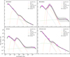 |
Fig. 10 Best-fit models. The target names are indicated in the top left corners of each panel. Individual components (star, hot dust, warm or cold dust, and stellar wind or Bremsstrahlung) are indicated by the blue, orange, red, and green lines, respectively. The combination of the models (best fit) are shown in bold black lines. The grey area encloses the combined uncertainties of the fitting. The magenta dots with error bars depict the de-reddened photometry. The four charts are depicted with the same wavelength and flux density scales to facilitate the comparison among the targets. |
6 Concluding remarks
We detected the central sources in four out of the five surveyed LBVs at both millimetre bands. We also found extended emission that reaches up to some 1–2 pc from the stars, although not all the features seem to be clearly associated with the targets. This is a step forward in the field because the millimetre continuum has only been observed in a handful of massive stars (Leitherer & Robert 1991; Higgs et al. 1994; Agliozzo et al. 2017b, 2019; Fenech et al. 2018).
With the 30 m beam size at the NIKA2 frequencies, our data can resolve structures that are typically larger than ~104 au at the distances of our targets. We distinguished several features in the millimetre maps: (1) unresolved sources, corresponding to the stellar winds, probably enshrouded by ionised gas and dust; (2) a plateau of extended emission, particularly noted in HD 168625; (3) a totally detached shell in G79.29+0.46; (4) some Galactic clouds that are not clearly linked to the stars; and (5) the IRDC in the G79.29+0.46 field.
These features may be characterised not only by their morphology, but also by their spectral indices (αmm). For the point sources, except for MN101, αmm is close to 0.6, which is the expected result for a canonical stellar wind. This trend becomes different when αmm is computed for the extended emission. The Galactic clouds in the fields of MN87 and MN101 and the IRDC in the field of G79.29+0.46 have the highest values of αmm (well above 2.5), which is typical of thermal dust emission. At the opposite end, there are the negative values found in the close environs of the central sources, where the stellar wind contribution seems diluted by more extended nebular material. In the field of G79.29+0.46, we noted two areas with clear gradients of αmm, from negative to positive values farther away from the position of the star; we propose an explanation of this behaviour by some sort of low-velocity shocks acting on one of the wellknown shells (Rizzo et al. 2008), and also in an interaction region with the IRDC (Palau et al. 2014).
In order to provide a better understanding of the relative importance of the excitation mechanisms, we complemented our NIKA2 data by an exhaustive search of archives, surveys, and dedicated observations available in the Virtual Observatory. For each target, we constructed six-decade SEDs with information from the visual to the radio regimes.
After we curated the data, we distinguished two types of SEDs that are determined by the relative flux density at millimetre wavelengths compared to their centimetre counterparts. The main feature of the first group (to which HD 168607 and G79.29+0.46 belong) is that the millimetre flux density is significantly higher (one order of magnitude) than the centimetre flux. In turn, the second group is characterised by comparable flux densities at millimetre and centimetre wavelengths. In the five cases we observed, the SEDs show that the sources are highly reddened and depict strong near- and mid-infrared emission.
We also proceeded with a (somewhat generic) modelling of the SEDs, with the objective of identifying different physical components and their relative contribution. The approach we used kept the number of components and parameters as small as possible. In this way, we were able to confirm or predict the existence of the modelled components, without including sophisticated information about structure, composition, or any other properties.
The fitting was satisfactory overall, considering that the data spanned six decades of the electromagnetic spectrum, the diversity of the instruments included, and the minimal number of free parameters employed. Notably, it allowed us to unveil unresolved hot-dust components at only four to six times the stellar radius in all cases but HD 168625, where the 500 K gas may extend up to 50–60 Rstar. It is known that these close-in structures are found in other massive evolved stars, such as B[e] supergiants, which are surrounded by circumstellar disks Zickgraf et al. (1985). In the context of LBV stars, the detection of au-sized hot-dust structures (500 to 2000 K) around active and quiescent sources may be explained by a dynamics where the ejecta expelled during a past mass-loss event falls back to the star, as proposed by some hydrodynamical simulations (Owocki 2013; Owocki et al. 2019). This fallback would produce dense rotating disks in which dust grains can survive against the hot radiation from the central star and grow efficiently, helped by self-shielding. Very high resolution IR and millimetre observations are needed to test this plausible but highly speculative interpretation.
In HD 168607, the mass-loss rate was better constrained by the combination of a better knowledge of its distance, the use of a measured wind velocity, and a fitting that considered the contribution of more extended cold dust.
The revised luminosity of HD 168625 would place it in the lowest part of the LBV zone in the HR diagram (Smith et al. 2004). This star has long been regarded as a twin of Sk-69 202, the blue supergiant identified as the progenitor of SN1987A (Walborn et al. 1987), owing to the striking similarities of their circumstellar material (Smith 2007). With the revised parameters from this work, the resemblance of HD 168625 and Sk-69 202 is even stronger: HD 168625 is nearly at the same position in the HR diagram as it was Sk-69 202 before the SN explosion (Smartt et al. 2002, see Fig. 6), that is, with nearly identical physical properties.
The non-detection of MN87 is intriguing. The upper limits for the central source at both NIKA2 frequencies are well below the expected fluxes from thermal cold dust or ionised gas. While a non-thermal contribution might help to explain these low fluxes, its inclusion is challenging considering the significant IR emission and the thermal spectral index of the central source at centimetre wavelengths (Ingallinera et al. 2016).
We presented the first estimates of the fundamental parameters of the central source of MN101. These results are compatible with a LBV close to its coldest value (Teff = 11 000 K). Its SED is very similar to that of HD 168625, although its hot-dust component is the most compact (1–2 au) and hottest of the sample (Tdust = 1800 K).
In G79.29+0.46, the sub-millimetre, millimetre, and centimetre-wavelength flux (and consequently, the energy input from the hot star) remained stationary during at least 22 years (see Higgs et al. 1994; Crossley et al. 2007; Umana et al. 2010, and our Appendix A.2). In the absence of a systematic photometric monitoring of G79.29+0.46, the apparent steadiness of the stellar wind and the dust properties strongly supports the candidate LBV status of this source (Voors et al. 2000).
It is remarkable that the stars that share a given type of SED also display similar Teff. Specifically, the two stars with a monotonically decrease from infrared to centimetre ranges (HD 168607 and G79.29+0.46) have the highest Teff, and their millimetre and centimetre SEDs are well-fitted only by stellar winds, while the other sources show the opposite behaviour (low Teff and free-free components). There is no clear explanation of this effect, although the sample is admittedly small for any conclusion.
This pilot study demonstrates the importance of studying the millimetre wavelength continuum emission in this type of object. The NIKA2 frequencies fall between the far-infrared and the radio domains, which are overall constrained by cold dust thermal emission and Bremsstrahlung mechanism, respectively. Therefore, the NIKA2 frequencies are very well suited to understand the relative contribution of these two mechanisms in detail, with the consequent determination of important parameters for the energy that is injected by the LBVs in their surrounding circumstellar material. Likewise, it suggests the existence of different families of SEDs that are closely tied to the stellar parameters. Follow-up works addressing a larger and statistically significant sample of LBV stars can shed further light on these aspects.
Acknowledgements
We would like to thank the IRAM staff for their kind and professional support during the observations and the NIKA2 core team for providing the data analysis software that was used to reconstruct the maps shown in the article. J.R.R. acknowledges support by PID2022-137779OB-C41 funded by MCIN/AEI/10.13039/501100011033 by “ERDF A way of making Europe”. This research has made use of the Spanish Virtual Observatory (https://svo.cab.inta-csic.es) project funded by MCIU/AEI/10.13039/501100011033/ through grant PID2023-146210NB-I00.
References
- Agliozzo, C., Noriega-Crespo, A., Umana, G., et al. 2014, MNRAS, 440, 1391 [NASA ADS] [CrossRef] [Google Scholar]
- Agliozzo, C., Nikutta, R., Pignata, G., et al. 2017a, MNRAS, 466, 213 [Google Scholar]
- Agliozzo, C., Trigilio, C., Pignata, G., et al. 2017b, ApJ, 841, 130 [Google Scholar]
- Agliozzo, C., Mehner, A., Phillips, N. M., et al. 2019, A&A, 626, A126 [NASA ADS] [CrossRef] [EDP Sciences] [Google Scholar]
- Arneson, R. A., Shenoy, D., Smith, N., & Gehrz, R. D. 2018, ApJ, 864, 31 [NASA ADS] [CrossRef] [Google Scholar]
- Bailer-Jones, C. A. L., Rybizki, J., Fouesneau, M., Demleitner, M., & Andrae, R. 2021, AJ, 161, 147 [Google Scholar]
- Blommaert, J. A. D. L., de Vries, B. L., Waters, L. B. F. M., et al. 2014, A&A, 565, A109 [NASA ADS] [CrossRef] [EDP Sciences] [Google Scholar]
- Bordiu, C., Rizzo, J. R., & Ritacco, A. 2019, MNRAS, 482, 1651 [CrossRef] [Google Scholar]
- Bordiu, C., Bufano, F., Cerrigone, L., et al. 2021, MNRAS, 500, 5500 [Google Scholar]
- Bordiu, C., Rizzo, J. R., Bufano, F., et al. 2022, ApJ, 939, L30 [NASA ADS] [CrossRef] [Google Scholar]
- Bordiu, C., Riggi, S., Bufano, F., et al. 2025, A&A, 695, A144 [NASA ADS] [CrossRef] [EDP Sciences] [Google Scholar]
- Buemi, C. S., Trigilio, C., Leto, P., et al. 2017, MNRAS, 465, 4147 [NASA ADS] [CrossRef] [Google Scholar]
- Chambers, K., & Pan-STARRS Team 2018, in American Astronomical Society Meeting Abstracts, 231, 102.01 [NASA ADS] [Google Scholar]
- Chen, X., Wang, S., Deng, L., et al. 2020, ApJS, 249, 18 [NASA ADS] [CrossRef] [Google Scholar]
- Clark, J. S., Najarro, F., Negueruela, I., et al. 2012, A&A, 541, A145 [NASA ADS] [CrossRef] [EDP Sciences] [Google Scholar]
- Crossley, J. H., Sjouwerman, L. O., Fomalont, E. B., & Radziwill, N. M. 2007, in American Astronomical Society Meeting Abstracts, 211, American Astronomical Society Meeting Abstracts, 132.03 [Google Scholar]
- Cutri, R. M., Wright, E. L., Conrow, T., et al. 2012, Explanatory Supplement to the WISE All-Sky Data Release Products [Google Scholar]
- Cutri, R. M., Wright, E. L., Conrow, T., et al. 2013, Explanatory Supplement to the AllWISE Data Release Products [Google Scholar]
- Draine, B. T., & Lee, H. M. 1984, ApJ, 285, 89 [NASA ADS] [CrossRef] [Google Scholar]
- Duncan, R. A., & White, S. M. 2002, MNRAS, 330, 63 [CrossRef] [Google Scholar]
- Egan, M. P., Price, S. D., Kraemer, K. E., et al. 2003, VizieR On-line Data Catalog: V/114 [Google Scholar]
- Elia, D., Molinari, S., Schisano, E., et al. 2017, MNRAS, 471, 100 [NASA ADS] [CrossRef] [Google Scholar]
- ESA. 1997, in ESA Special Publications, 1200, (Noordwijk: ESA) [Google Scholar]
- Fenech, D. M., Clark, J. S., Prinja, R. K., et al. 2018, A&A, 617, A137 [NASA ADS] [CrossRef] [EDP Sciences] [Google Scholar]
- Flagey, N., Noriega-Crespo, A., Petric, A., & Geballe, T. R. 2014, AJ, 148, 34 [NASA ADS] [CrossRef] [Google Scholar]
- Forbrich, J., Öberg, K., Lada, C. J., et al. 2014, A&A, 568, A27 [NASA ADS] [CrossRef] [EDP Sciences] [Google Scholar]
- Friesen, R. K., Pon, A., Bourke, T. L., et al. 2018, ApJ, 869, 158 [NASA ADS] [CrossRef] [Google Scholar]
- Gaia Collaboration 2022, VizieR On-line Data Catalog: I/355 [Google Scholar]
- Gordon, Y. A., Boyce, M. M., O’Dea, C. P., et al. 2021, ApJS, 255, 30 [NASA ADS] [CrossRef] [Google Scholar]
- Green, G. 2018, J. Open Source Softw., 3, 695 [NASA ADS] [CrossRef] [Google Scholar]
- Green, G. M., Schlafly, E., Zucker, C., Speagle, J. S., & Finkbeiner, D. 2019, ApJ, 887, 93 [NASA ADS] [CrossRef] [Google Scholar]
- Gull, T. R., Morris, P. W., Black, J. H., et al. 2020, MNRAS, 499, 5269 [NASA ADS] [CrossRef] [Google Scholar]
- Gutermuth, R. A., & Heyer, M. 2015, AJ, 149, 64 [Google Scholar]
- Gvaramadze, V. V., Kniazev, A. Y., & Fabrika, S. 2010, MNRAS, 405, 1047 [NASA ADS] [Google Scholar]
- Hale, C. L., McConnell, D., Thomson, A. J. M., et al. 2021, PASA, 38, e058 [NASA ADS] [CrossRef] [Google Scholar]
- Heinze, A. N., Tonry, J. L., Denneau, L., et al. 2018, AJ, 156, 241 [Google Scholar]
- Helfand, D. J., Becker, R. H., White, R. L., Fallon, A., & Tuttle, S. 2006, AJ, 131, 2525 [Google Scholar]
- Helou, G., & Walker, D. W. 1988, in Infrared Astronomical Satellite (IRAS) Catalogs and Atlases 7 [Google Scholar]
- Higgs, L. A., Wendker, H. J., & Landecker, T. L. 1994, A&A, 291, 295 [NASA ADS] [Google Scholar]
- Humphreys, R. M., & Davidson, K. 1994, PASP, 106, 1025 [NASA ADS] [CrossRef] [Google Scholar]
- Hutsemekers, D., van Drom, E., Gosset, E., & Melnick, J. 1994, A&A, 290, 906 [NASA ADS] [Google Scholar]
- Ingallinera, A., Trigilio, C., Umana, G., et al. 2014, MNRAS, 437, 3626 [Google Scholar]
- Ingallinera, A., Trigilio, C., Leto, P., et al. 2016, MNRAS, 463, 723 [NASA ADS] [CrossRef] [Google Scholar]
- Ishihara, D., Onaka, T., Kataza, H., et al. 2010, A&A, 514, A1 [NASA ADS] [CrossRef] [EDP Sciences] [Google Scholar]
- Jiménez-Esteban, F. M., Rizzo, J. R., & Palau, A. 2010, ApJ, 713, 429 [Google Scholar]
- Jones, A. P., Fanciullo, L., Köhler, M., et al. 2013, A&A, 558, A62 [NASA ADS] [CrossRef] [EDP Sciences] [Google Scholar]
- Kochanek, C. S. 2011, ApJ, 743, 73 [NASA ADS] [CrossRef] [Google Scholar]
- Kraemer, K. E., Hora, J. L., Egan, M. P., et al. 2010, AJ, 139, 2319 [Google Scholar]
- Langer, N., Hamann, W. R., Lennon, M., et al. 1994, A&A, 290, 819 [NASA ADS] [Google Scholar]
- Lasker, B. M., Lattanzi, M. G., McLean, B. J., et al. 2008, AJ, 136, 735 [Google Scholar]
- Leitherer, C., & Robert, C. 1991, ApJ, 377, 629 [Google Scholar]
- Leitherer, C., Chapman, J. M., & Koribalski, B. 1995, ApJ, 450, 289 [NASA ADS] [CrossRef] [Google Scholar]
- Mahy, L., Hutsemékers, D., Royer, P., & Waelkens, C. 2016, A&A, 594, A94 [NASA ADS] [CrossRef] [EDP Sciences] [Google Scholar]
- Marocco, F., Eisenhardt, P. R. M., Fowler, J. W., et al. 2021, ApJS, 253, 8 [Google Scholar]
- Martayan, C., Lobel, A., Baade, D., et al. 2016, A&A, 587, A115 [NASA ADS] [CrossRef] [EDP Sciences] [Google Scholar]
- Mathis, J. S., Rumpl, W., & Nordsieck, K. H. 1977, ApJ, 217, 425 [Google Scholar]
- Mezger, P. G., & Henderson, A. P. 1967, ApJ, 147, 471 [Google Scholar]
- Mizuno, D. R., Kraemer, K. E., Flagey, N., et al. 2010, AJ, 139, 1542 [NASA ADS] [CrossRef] [Google Scholar]
- Molinari, S., Swinyard, B., Bally, J., et al. 2010, PASP, 122, 314 [Google Scholar]
- Molinari, S., Schisano, E., Elia, D., et al. 2016, A&A, 591, A149 [NASA ADS] [CrossRef] [EDP Sciences] [Google Scholar]
- Morris, P. W., Charnley, S. B., Corcoran, M., et al. 2020, ApJ, 892, L23 [NASA ADS] [CrossRef] [Google Scholar]
- O’Hara, T. B., Meixner, M., Speck, A. K., Ueta, T., & Bobrowsky, M. 2003, ApJ, 598, 1255 [Google Scholar]
- Ossenkopf, V., & Henning, T. 1994, A&A, 291, 943 [NASA ADS] [Google Scholar]
- Owocki, S. 2013, Stellar Winds, eds. T. D. Oswalt, & M. A. Barstow (Dordrecht: Springer Netherlands), 735 [Google Scholar]
- Owocki, S. P., Hirai, R., Podsiadlowski, P., & Schneider, F. R. N. 2019, MNRAS, 485, 988 [NASA ADS] [CrossRef] [Google Scholar]
- Paegert, M., Stassun, K. G., Collins, K. A., et al. 2022, VizieR On-line Data Catalog: IV/39 [Google Scholar]
- Palau, A., Rizzo, J. R., Girart, J. M., & Henkel, C. 2014, ApJ, 784, L21 [NASA ADS] [CrossRef] [Google Scholar]
- Panagia, N., & Felli, M. 1975, A&A, 39, 1 [Google Scholar]
- Perotto, L., Ponthieu, N., Macías-Pérez, J. F., et al. 2020, A&A, 637, A71 [NASA ADS] [CrossRef] [EDP Sciences] [Google Scholar]
- Planck Collaboration XI. 2014, A&A, 571, A11 [NASA ADS] [CrossRef] [EDP Sciences] [Google Scholar]
- Purcell, C. R., Hoare, M. G., Cotton, W. D., et al. 2013, ApJS, 205, 1 [Google Scholar]
- Rizzo, J. R., Jiménez-Esteban, F. M., & Ortiz, E. 2008, ApJ, 681, 355 [CrossRef] [Google Scholar]
- Rizzo, J. R., Palau, A., Jiménez-Esteban, F., & Henkel, C. 2014, A&A, 564, A21 [NASA ADS] [CrossRef] [EDP Sciences] [Google Scholar]
- Rizzo, J. R., Bordiu, C., Buemi, C., et al. 2023, A&A, 678, A55 [NASA ADS] [CrossRef] [EDP Sciences] [Google Scholar]
- Schlafly, E. F., Meisner, A. M., & Green, G. M. 2019, ApJS, 240, 30 [Google Scholar]
- Skrutskie, M. F., Cutri, R. M., Stiening, R., et al. 2006, AJ, 131, 1163 [NASA ADS] [CrossRef] [Google Scholar]
- Smartt, S. J., Lennon, D. J., Kudritzki, R. P., et al. 2002, A&A, 391, 979 [NASA ADS] [CrossRef] [EDP Sciences] [Google Scholar]
- Smith, N. 2007, AJ, 133, 1034 [NASA ADS] [CrossRef] [Google Scholar]
- Smith, N. 2013, MNRAS, 429, 2366 [Google Scholar]
- Smith, N., Vink, J. S., & de Koter, A. 2004, ApJ, 615, 475 [NASA ADS] [CrossRef] [Google Scholar]
- Spitzer Science Center (SSC) 2009, VizieR On-line Data Catalog: II/293 [Google Scholar]
- Spitzer Science Center (SSC) & Infrared Science Archive (IRSA) 2021, VizieR On-line Data Catalog: II/368 [Google Scholar]
- Umana, G., Buemi, C. S., Trigilio, C., & Leto, P. 2005, A&A, 437, L1 [NASA ADS] [CrossRef] [EDP Sciences] [Google Scholar]
- Umana, G., Buemi, C. S., Trigilio, C., Leto, P., & Hora, J. L. 2010, ApJ, 718, 1036 [NASA ADS] [CrossRef] [Google Scholar]
- Umana, G., Buemi, C. S., Trigilio, C., et al. 2011, ApJ, 739, L11 [NASA ADS] [CrossRef] [Google Scholar]
- Umana, G., Ingallinera, A., Trigilio, C., et al. 2012, MNRAS, 427, 2975 [NASA ADS] [CrossRef] [Google Scholar]
- Vamvatira-Nakou, C., Hutsemékers, D., Royer, P., et al. 2013, A&A, 557, A20 [NASA ADS] [CrossRef] [EDP Sciences] [Google Scholar]
- Vamvatira-Nakou, C., Hutsemékers, D., Royer, P., et al. 2015, A&A, 578, A108 [NASA ADS] [CrossRef] [EDP Sciences] [Google Scholar]
- Voors, R. H. M., Geballe, T. R., Waters, L. B. F. M., Najarro, F., & Lamers, H. J. G. L. M. 2000, A&A, 362, 236 [NASA ADS] [Google Scholar]
- Wachter, S., Mauerhan, J. C., Van Dyk, S. D., et al. 2010, AJ, 139, 2330 [NASA ADS] [CrossRef] [Google Scholar]
- Wachter, S., Mauerhan, J., van Dyk, S., Hoard, D. W., & Morris, P. 2011, Bull. Soc. Roy. Sci. Liege, 80, 291 [NASA ADS] [Google Scholar]
- Walborn, N. R., Lasker, B. M., Laidler, V. G., & Chu, Y.-H. 1987, ApJ, 321, L41 [NASA ADS] [CrossRef] [Google Scholar]
- Wang, Y., Beuther, H., Rugel, M. R., et al. 2020, A&A, 634, A83 [NASA ADS] [CrossRef] [EDP Sciences] [Google Scholar]
- Waters, L. B. F. M., Izumiura, H., Zaal, P. A., et al. 1996, A&A, 313, 866 [NASA ADS] [Google Scholar]
- Weis, K. 2001, Rev. Mod. Astron., 14, 261 [NASA ADS] [Google Scholar]
- Weis, K. 2011, in Active OB Stars: Structure, Evolution, Mass Loss, and Critical Limits, 272, eds. C. Neiner, G. Wade, G. Meynet, & G. Peters, 372 [Google Scholar]
- Wright, A. E., & Barlow, M. J. 1975, MNRAS, 170, 41 [Google Scholar]
- Yang, A. Y., Dzib, S. A., Urquhart, J. S., et al. 2023, A&A, 680, A92 [NASA ADS] [CrossRef] [EDP Sciences] [Google Scholar]
- Zickgraf, F. J., Wolf, B., Stahl, O., Leitherer, C., & Klare, G. 1985, A&A, 143, 421 [Google Scholar]
- Zylka, R. 2013, MOPSIC: Extended Version of MOPSI, Astrophysics Source Code Library [record ascl:1303.011] [Google Scholar]
Appendix A Spectral energy distributions
Appendix A.1 Data origin
In Table A.1 we detail basic information about the catalogues, surveys, and observations used to build the SEDs.
Surveys and catalogues.
Appendix A.2 Data notes on individual sources
In this section we report some particular notes which complement the information presented in the SEDs.
HD168607 (Figure 5)
Pan-STARRS photometry shows significant dispersion (up to a factor of 4 in g) so it was discarded.
The WISE band 4 measurement is heavily contaminated by nearby extended emission not related to the star. As no reliable flux could be determined, the measurement was discarded.
We found point like emission at 70 and 100 μm with Herschel/PACS. The nearby HD168625 is a target of a project (observation IDs from 1342217763 to 1342217766), and the observed images include by chance the position of HD168607. We extracted a field around HD168607 from the original images and fitted a two-dimensional Gaussian source. The results are shown in Fig. A.1 and in Table A.2. At 160 μm the star is no longer detected.
This source is catalogued in the GLOSTAR survey at 1.4 GHz (Yang et al. 2023), but not in CORNISH, MAGPIS, or THOR. In the search for references not available in VizieR, we found a survey made with ATCA at 8.54 GHz (Leitherer et al. 1995), which was added to the SED.
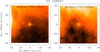 |
Fig. A.1 Herschel/PACS images around HD168607 at 70 μm (left) and 100 μm (right). Equatorial coordinates are relative to the star position. The continuum emission at these wavelengths is reported for the first time in this work. |
Fitting of the PACS mid-IR fluxes of HD168607.
HD168625 (Figure 6)
The source is included in the IRAS Point Source Catalogue, although not detected at 100 μm.
In the PACS images at 70 and 100 μm the star is not detected. In Hi-Gal, the nebula is listed as two different sources (the brightest parts of the nebula); we consequently summed up the two fluxes, and assumed uncertainties of 10%.
A complete study in the infrared was done by Arneson et al. (2018), who included their SOFIA measurements together with 2MASS, AKARI, WISE, MSX, Spitzer and Herschel data. We cross-checked the spectral fluxes in the paper with our ones obtained from VizieR, and added the SOFIA and Herschel/PACS data to our SED.
The WISE band 4 flux is clearly overestimated, up to three times the fluxes of MIPS, MSX, IRAS and AKARI in nearby wavelengths. Such effect is probably due to the large aperture of WISE at 22 μm, which is critical in presence of the strong IR nebula. We therefore remove this point from the SED.
The source is not included in the THOR catalogue, but we downloaded the images and detected some extended emission. We averaged three frequencies (1690, 1820 and 1950 MHz) to get a reliable source detection, and incorporated the average to the SED. This source was also observed by Leitherer et al. (1995) at 8.54 GHz using ATCA, and we therefore also included those measured values.
Umana et al. (2010) observed this target at high resolution with the VLA at 8.54 GHz, detecting the central point source (0.42 mJy) while resolving out most of the extended nebula; we therefore decided to take this measurement into account for the fitting, as explained below. The VLASS survey also detected this point source at 2–4 GHz, with a surrounding ring of 5–10 arcsec.
After a close inspection to the data, we noted that the THOR flux is higher than the adjacent ones. We explored whether this is due to an incorrect flux measurement6, or due to the possibility of reaching the turnover frequency close to the VLASS frequency (3 GHz). To do so, we downloaded and analysed the individual images available in the THOR Image Server7. These images correspond to epochs 1.2 and 2.2, but only in the first one the source is detected. Our measured flux is compatible with that provided in the archive, so we confirm its validity and used the tabulated value and its uncertainty.
MN101 (Figure 8)
The Gaia G flux is anomalously high with respect to the other Gaia bands, and significantly above measurements of other surveys. This effect may be due to the presence of circumstellar dust which contaminates the star photometry, as explained in Sect. 4.2.
This source is included in most of the radio surveys searched. The flux densities from THOR were quite discrepant with respect to others, so we recomputed them using aperture photometry. Our values are more consistent with the other surveys, and we therefore decided to incorporate them to the SED, instead of the catalogued ones.
The nebular feature was observed with the VLA (Ingallinera et al. 2014) at 1.4 and 5 GHz, with flux densities of 10.2 ± 0.8 and 10.5 ± 0.1 mJy, respectively. Considering that the angular extent of the source (~20 arcsec) is comparable to the NIKA2 beam, we preferred these values for the fitting. Higher resolution 5 GHz observations by Ingallinera et al. (2016) revealed a central point source (7.0 ± 0.2 mJy), with a spectral index compatible with a thermal stellar wind and an ionised circumstellar material characterised by a non-thermal spectral index.
G79.29+0.46 (Figure 9)
The source is highly reddened. G79.29+0.46 has been observed in three different epochs by SDSS; the measurements differ up to a factor of two, probably due to stellar variability. The PAN-STARRS survey, made some years after the SDSS data release, shows a similar behaviour. In fact, G79.29+0.46 is included in the catalogues of Heinze et al. (2018) and Chen et al. (2020) of variable stars. We decided to keep different points for SDSS and PAN-STARRS to reflect the source variability.
Agliozzo et al. (2014, referred to as Agl14 in the SED) observed this source at 8.46, 4.96, and 1.4 GHz using the VLA interferometer, and made a SED study in the infrared domain using observations of Herschel, Spitzer, ISO and WISE. We cross-checked our values in common (e.g., from WISE and 2MASS) and completed our SED by incorporating their values from Spitzer and Herschel.
VLASS does not include this source in its catalogue, although it is noted some point-like emission in the images corresponding to the three epochs observed. We therefore computed the integrated fluxes and averaged them with a inverse-square weighting of the flux uncertainties.
The NVAS archive also provides images in the C-, X-, K-, and Q-bands. We computed the integrated fluxes in these images as well, and incorporated them to the SED. The flux uncertainties in C- and X-bands are notoriously large in comparison to those of the targetted observations of Agliozzo et al. (2014) at similar frequencies; we therefore decided to keep these NVAS data in the SED, but remove them as input for the fitting.
Higgs et al. (1994) made a multi-wavelength study of the central source and the surrounding shells, including data from IRAS and targetted observations of several instruments from 0.8 mm to 5 GHz. The fluxes measured at all these frequencies are consistent with our NIKA2 values and the above mentioned radio surveys (NVAS, VLASS, Agl14), which demonstrates that G79.29+0.46 remained stationary at centimetre- and millimetre-wavelengths at least during the last 20 years.
Appendix B Modelling details
Central star
The contribution of the star was modelled as a black body, parametrised by the effective temperature Teff, the stellar radius Rstar, and the distance d to the star. In this way, the flux density is:
![Mathematical equation: $\[S_\nu=\Omega ~B_\nu(T_{\text {eff}})=\Omega \frac{2~ h ~\nu^3 / c^2}{\exp \left(h ~\nu / k ~T_{\text {eff }}\right)-1}\]$](/articles/aa/full_html/2025/11/aa55449-25/aa55449-25-eq9.png) (B.1)
(B.1)
with Ω being the solid angle subtended by the source, Ω = π (Rstar/d)2, and Bν(Teff) the Planck function.
The simplicity of this model is adequate for the purpose of this article. The uncertainties introduced by this simplification is by far below those due to the variability of the stars and the heterogeneity of the collected visual and near-infrared data. This fitting is sufficient to provide good approximations of Teff and Rstar, and to constrain the neighbour range of wavelengths, where the hot dust is dominant.
Circumstellar dust
The emission arising from this component was modelled by modified black bodies (sometimes referred to as grey bodies), parametrised by a dust temperature Tdust, a characteristic radius of the emitting region Rdust (expected much larger than Rstar), and a dust opacity law (Ossenkopf & Henning 1994):
![Mathematical equation: $\[\kappa_\nu=\kappa_0\left(\nu / \nu_0\right)^\beta\]$](/articles/aa/full_html/2025/11/aa55449-25/aa55449-25-eq10.png) (B.2)
(B.2)
In the above equation, κν is the dust mass opacity in units of cm2 g−1, κ0 is the dust opacity at the reference frequency ν0 (here chosen at 230 GHz) and β is the dust emissivity index. The measured flux density of the modified black body results:
![Mathematical equation: $\[S_\nu=\sigma ~\kappa_\nu \mathrm{~B}_\nu(T_{\text {dust}}) ~\Omega_{\text {cloud }}\]$](/articles/aa/full_html/2025/11/aa55449-25/aa55449-25-eq11.png) (B.3)
(B.3)
where σ is the dust mass column density along the line of sight (in units of g cm−2) and Ωcloud the solid angle subtended by the cloud of radius Rdust. If the total dust mass of the cloud is Mdust, we can roughly compute
![Mathematical equation: $\[\begin{gathered}\sigma=\frac{M_{\text {dust }}}{\pi ~R_{\text {dust }}^2} \\\kappa_\nu=\kappa_{\nu_0}(\nu / \nu_0)^\beta=\kappa_{\nu_0}(\lambda_0 / \lambda)^\beta \\\Omega=\pi(R_{\text {dust }} / d)^2\end{gathered}\]$](/articles/aa/full_html/2025/11/aa55449-25/aa55449-25-eq12.png)
and the flux density results:
![Mathematical equation: $\[S_\nu=M_{\text {dust}} ~\kappa_0 ~\lambda_0^\beta ~\lambda^{-\beta} \mathrm{B}_\nu(T_{\text {dust}}) / d^2\]$](/articles/aa/full_html/2025/11/aa55449-25/aa55449-25-eq13.png) (B.4)
(B.4)
For low to moderate gas densities, dust opacities of MRN grain (Mathis et al. 1977) with and without ice mantles ranges from 0.3 to 0.9 cm2 g−1. So far, we estimated the dust masses in Table 3 by assuming κ0 = 0.5 cm2 g−1, which yields uncertainties due to unknown κ0 within a factor of two. In this way, the can fit the density flux arising from a dust cloud in terms of β, Mdust, and Tdust.
The parameter β encapsulates key dust properties, such as composition, porosity, and grain size distribution. Therefore, single-β grey bodies are just a simplification without a specific physical meaning (Jones et al. 2013). Even so, they provide useful information about the dust behaviour. In our modelling we considered β as a free parameter, although it was indeed necessary only for the cold component of HD168625, where the best-fit was found for β = 1 ± 0.2. For the other cases, the best-fit value of β was zero, i.e., all other components are well-fitted as ideal black bodies.
When the best-fit corresponds to a black body, we can additionally derive Rdust because the density flux is also:
![Mathematical equation: $\[S_\nu=\mathrm{B}_\nu(T_{\text {dust}}) \Omega=\mathrm{B}_\nu(T_{\text {dust}}) \pi\left(R_{\text {dust}} / d\right)^2\]$](/articles/aa/full_html/2025/11/aa55449-25/aa55449-25-eq14.png) (B.5)
(B.5)
In practice, we fitted the SED through the expression:
![Mathematical equation: $\[S_\nu=\frac{1}{(\lambda / 1 \mu \mathrm{m})^\beta} ~\mathrm{B}_\nu(T_{\mathrm{dust}}) ~\pi~(\hat{R} / d)^2\]$](/articles/aa/full_html/2025/11/aa55449-25/aa55449-25-eq15.png) (B.6)
(B.6)
where ![Mathematical equation: $\[\hat{R}\]$](/articles/aa/full_html/2025/11/aa55449-25/aa55449-25-eq16.png) is considered as a fiducial radius. By equating Eqs. B.4 and B.6 we can derive, after some algebra, a relationship between Mdust and
is considered as a fiducial radius. By equating Eqs. B.4 and B.6 we can derive, after some algebra, a relationship between Mdust and ![Mathematical equation: $\[\hat{R}\]$](/articles/aa/full_html/2025/11/aa55449-25/aa55449-25-eq17.png) :
:
![Mathematical equation: $\[M_{\mathrm{dust}}=\frac{\pi ~\hat{R}^2}{\kappa_0~\left(\lambda_0 / 1 \mu \mathrm{m}\right)^\beta}\]$](/articles/aa/full_html/2025/11/aa55449-25/aa55449-25-eq18.png) (B.7)
(B.7)
When β ≠ 0, ![Mathematical equation: $\[\hat{R}\]$](/articles/aa/full_html/2025/11/aa55449-25/aa55449-25-eq19.png) is just a proxy to derive Mdust, without a real physical meaning. On the other hand, when the best-fit corresponds to a black body
is just a proxy to derive Mdust, without a real physical meaning. On the other hand, when the best-fit corresponds to a black body ![Mathematical equation: $\[(\beta=0) \hat{R}=R_{\text {dust}}\]$](/articles/aa/full_html/2025/11/aa55449-25/aa55449-25-eq20.png) . Due to the uncertainties and assumptions involved, the masses must be considered just as a rough approximation.
. Due to the uncertainties and assumptions involved, the masses must be considered just as a rough approximation.
Stellar wind
This component was modelled by a stationary, isotropic, and isothermal stellar wind, expanding at constant velocity (Panagia & Felli 1975; Wright & Barlow 1975). In the optically thick regime, the flux density of such a wind at the frequency ν is:
![Mathematical equation: $\[\begin{aligned}S_\nu~(\text {thick}) & =5.12\left(\frac{\nu}{10 ~\mathrm{GHz}}\right)^{0.6}\left(\frac{T_{\mathrm{e}}}{10^4 \mathrm{~K}}\right)^{0.1}\left(\frac{\dot{M}}{10^{-5} ~\mathrm{M}_{\odot} / \mathrm{yr}}\right)^{4 / 3} \\& \times\left(\frac{\mu}{1.2}\right)^{-4 / 3}\left(\frac{\nu_{\infty}}{10^3 \mathrm{~km} / \mathrm{s}}\right)^{-4 / 3}(\bar{Z})^{2 / 3}\left(\frac{d}{\mathrm{kpc}}\right)^{-2} ~\mathrm{mJy}\end{aligned}\]$](/articles/aa/full_html/2025/11/aa55449-25/aa55449-25-eq21.png) (B.8)
(B.8)
where Te is the electronic temperature, ![Mathematical equation: $\[\dot{M}\]$](/articles/aa/full_html/2025/11/aa55449-25/aa55449-25-eq22.png) the mass-loss rate, μ the mean molecular weight (assumed 1.2), v∞ the expansion velocity of the wind, and
the mass-loss rate, μ the mean molecular weight (assumed 1.2), v∞ the expansion velocity of the wind, and ![Mathematical equation: $\[\bar{Z}\]$](/articles/aa/full_html/2025/11/aa55449-25/aa55449-25-eq23.png) the average ionic charge (assumed 1). The optically thick assumption holds up to a certain turnover frequency νc, equal to
the average ionic charge (assumed 1). The optically thick assumption holds up to a certain turnover frequency νc, equal to
![Mathematical equation: $\[\nu_c=4.7 \times 10^{42} \frac{\gamma^{1 / 2} g_{\mathrm{ff}}^{1 / 2} \bar{Z}}{T_{\mathrm{e}}^{3 / 4} R_{\mathrm{c}}^{3 / 2}} \frac{\dot{M}}{\mu ~v_{\infty}} \mathrm{Hz}\]$](/articles/aa/full_html/2025/11/aa55449-25/aa55449-25-eq24.png) (B.9)
(B.9)
with γ being the number of electrons per ion and gff the free-free Gaunt factor, approximated as Leitherer & Robert (1991):
![Mathematical equation: $\[g_{\mathrm{ff}}=9.77\left(1+0.13 ~\log~ \frac{T_{\mathrm{e}}^{3 / 2}}{{\bar{Z}~\nu}}\right)\]$](/articles/aa/full_html/2025/11/aa55449-25/aa55449-25-eq25.png) (B.10)
(B.10)
and Rc denoting the inner boundary radius of the ionised envelope (here assumed equal to Rstar). Above νc the spectrum begins to flatten, approaching that of an optically thin H II region with α = −0.1. In this regime, the flux density results:
![Mathematical equation: $\[S_\nu~(\text {thin})=S_{\nu_c} ~(\nu / \nu_c)^{-0.1}\]$](/articles/aa/full_html/2025/11/aa55449-25/aa55449-25-eq26.png) (B.11)
(B.11)
We may note in Eq. (B.8) the weak dependence of the flux density with Te. In any case, we tested different models by varying Te from 103 to 105 K and noted that the changes in the flux were always smaller than the uncertainties of the observed fluxes. We therefore adopted Te = 104 K to avoid an unnecessary free parameter. Finally, there is a degeneracy in ![Mathematical equation: $\[\dot{M}\]$](/articles/aa/full_html/2025/11/aa55449-25/aa55449-25-eq27.png) and v∞ because the flux density varies with (
and v∞ because the flux density varies with (![Mathematical equation: $\[\dot{M}\]$](/articles/aa/full_html/2025/11/aa55449-25/aa55449-25-eq28.png) /v∞)4/3. For simplicity, we adopted v∞ = 100 km s−1 and leave
/v∞)4/3. For simplicity, we adopted v∞ = 100 km s−1 and leave ![Mathematical equation: $\[\dot{M}\]$](/articles/aa/full_html/2025/11/aa55449-25/aa55449-25-eq29.png) as the only free parameter.
as the only free parameter.
There is a circular dependence between νc and gff because νc is frequency-dependent through gff. It is therefore necessary to adopt a fixed value of gff. The Gaunt factor gff varies roughly from 2 to 6 within its validity range (from centimetre to millimetre wavelengths), while νc falls in the mid-IR range. Consequently, we adopted a characteristic gff = 4.08, corresponding to a frequency of 30 GHz, for the calculation of νc. This causes an uncertainty in the turnover frequency up to a factor of 2, which has no significant impact on the millimetre/centimetre fluxes.
Bremsstrahlung
For this component, we modelled the free-free emission from an ionised, static, and isothermal H II region characterised by a radius Rff. In the optically thin regime (Mezger & Henderson 1967), the flux density behaves as:
![Mathematical equation: $\[S_\nu~(\text {thin})=2 ~k ~T_{\mathrm{e}}\left(\frac{\nu}{c}\right)^2 \tau ~\Omega_{\mathrm{ff}}\]$](/articles/aa/full_html/2025/11/aa55449-25/aa55449-25-eq30.png) (B.12)
(B.12)
Ωff = π (Rff/d)2 is the solid angle of the ionised region and τ is the optical depth, given by
![Mathematical equation: $\[\tau=3.28 \times 10^{-7}\left(\frac{T_{\mathrm{e}}}{10^4 \mathrm{~K}}\right)^{-1.35}\left(\frac{\nu}{\mathrm{GHz}}\right)^{-2.1}\left(\frac{E M}{\mathrm{pc} \mathrm{~cm}^{-6}}\right)\]$](/articles/aa/full_html/2025/11/aa55449-25/aa55449-25-eq31.png) (B.13)
(B.13)
where EM represents the emission measure of the ionised region.
Solving Eq. (B.13) for τ = 1, it is possible to compute the turnover frequency νc. At frequencies below νc, the H II region enters in the optically thick regime, the spectrum steepens, and it follows the Rayleigh-Jeans approximation (Sν ∝ ν2).
See Lacy et al. 2019, VLASS Project Memo #13: Pilot and Epoch 1 Quick Look Data Release https://library.nrao.edu/public/memos/vla/vlass/VLASS_013.pdf.
All Tables
All Figures
|
Fig. 1 Noise map of the observed fields. The rms noise was computed in concentric rings with a width of 2 arcsec. The noise in the 1.15 mm maps is plotted in blue, and the noise corresponding to the 2 mm maps is plotted in red. The field names (abridged) are indicated near the 1 mm curves. |
| In the text | |
|
Fig. 2 Sky maps of the millimetre continuum emission in the four fields observed with NIKA2. The maps at 1.15 mm are shown at the top row, and the 2 mm maps are shown at the bottom. The field that contains HD 168607 and HD 168625, labelled HD168*, is centred on HD 168625. The colour scales (indicated at the right of each row) are in Jy beam−1. HPBWs are drawn near the bottom left corners of the HD168* images. The central areas indicate the zoomed region displayed in Fig. 3. |
| In the text | |
|
Fig. 3 Zoomed sky maps around the central sources. The regions correspond to the regions indicated in Fig. 2. To span the full dynamic range, the colour scale is different for each of the maps. The contours correspond to 30, 50 (highlighted in white), and 70% of the maximum value. HPBWs are indicated near the bottom of the HD168* images. The contours at 50% are highlighted to facilitate a visual comparison with the beam and give an idea about the point-like nature of the central sources. |
| In the text | |
|
Fig. 4 Spectral index maps between the two NIKA2 frequencies. The plotted field and marks are the same as in Fig. 2. For each map, all pixels with brightness below 2σ were masked. |
| In the text | |
|
Fig. 5 Spectral energy distribution of HD 168607 in logarithmic scale. The catalogues are indicated at the top right. The corresponding error bars of all points are plotted. The NIKA2 points are shown with blue stars. |
| In the text | |
|
Fig. 6 Spectral energy distribution of HD 168625. |
| In the text | |
|
Fig. 7 Spectral energy distribution of [GKF2010]MN87. |
| In the text | |
|
Fig. 8 Spectral energy distribution of [GKF2010]MN101. |
| In the text | |
|
Fig. 9 Spectral energy distribution of G79.29+0.46. |
| In the text | |
|
Fig. 10 Best-fit models. The target names are indicated in the top left corners of each panel. Individual components (star, hot dust, warm or cold dust, and stellar wind or Bremsstrahlung) are indicated by the blue, orange, red, and green lines, respectively. The combination of the models (best fit) are shown in bold black lines. The grey area encloses the combined uncertainties of the fitting. The magenta dots with error bars depict the de-reddened photometry. The four charts are depicted with the same wavelength and flux density scales to facilitate the comparison among the targets. |
| In the text | |
|
Fig. A.1 Herschel/PACS images around HD168607 at 70 μm (left) and 100 μm (right). Equatorial coordinates are relative to the star position. The continuum emission at these wavelengths is reported for the first time in this work. |
| In the text | |
Current usage metrics show cumulative count of Article Views (full-text article views including HTML views, PDF and ePub downloads, according to the available data) and Abstracts Views on Vision4Press platform.
Data correspond to usage on the plateform after 2015. The current usage metrics is available 48-96 hours after online publication and is updated daily on week days.
Initial download of the metrics may take a while.