| Issue |
A&A
Volume 703, November 2025
|
|
|---|---|---|
| Article Number | A134 | |
| Number of page(s) | 10 | |
| Section | Astrophysical processes | |
| DOI | https://doi.org/10.1051/0004-6361/202555561 | |
| Published online | 13 November 2025 | |
Gaussian process analysis of type-B quasiperiodic oscillations in the black hole X-ray binary MAXI J1348–630
1
School of Physics and Technology, Wuhan University, Wuhan, Hubei 430072, People’s Republic of China
2
School of Physics and Astronomy, University of Southampton, Highfield, Southampton SO17 1BJ, UK
3
Yunnan Key Laboratory of Statistical Modeling and Data Analysis, Yunnan University, Kunming, Yunnan 650091, People’s Republic of China
4
Department of Astronomy, Key Laboratory of Astroparticle Physics of Yunnan Province, Yunnan University, Kunming, Yunnan 650091, People’s Republic of China
⋆ Corresponding author: This email address is being protected from spambots. You need JavaScript enabled to view it.
, This email address is being protected from spambots. You need JavaScript enabled to view it.
Received:
17
May
2025
Accepted:
15
September
2025
Abstract
We analyzed Insight-HXMT data of the black hole X-ray binary MAXI J1348–630 during the type-B quasiperiodic oscillation (QPO) phase of its 2019 outburst. Using the Gaussian process method, we applied an additive composite kernel model consisting of a stochastically driven damped simple harmonic oscillator (SHO), a damped random walk (DRW), and an additional white noise (AWN) to data from three energy bands: low energy (LE; 1–10 keV) band, medium energy (ME; 10–30 keV) band, and high energy (HE; 30–150 keV) band. We find that for the DRW component, correlations on the timescale of τDRW ∼ 10 s are absent in the LE band, while they persist in the ME and HE bands over the full duration of the light curves. This energy-dependent behavior may reflect thermal instabilities, with the shorter correlation timescale in the disk compared to the corona. Alternatively, it may reflect variable Comptonizations of seed photons from different disk regions. Inner-disk photons are scattered by a small inner corona, producing soft X-rays. Outer-disk photons interact with an extended, jet-like corona, resulting in harder emission. The QPO is captured by an SHO component with a stable period of ∼0.2 s and a high quality factor of ∼10. The absence of significant evolution with energy or time of the SHO component suggests a connection between the accretion disk and the corona, which may be built by coherent oscillations of disk-corona driven by magnetorotational instability. The AWN components are present in all the three-band data and dominate over the DRW and SHO components. We interpret the AWN as another fast DRW with its τDRW < 0.01 s. It may trace high-frequency fluctuations that occur in both the inner region of the accretion disk and the corona. Overall, our work reveals a timescale hierarchy in the coupled disk-corona scenario: fast DRW < SHO < disk DRW < corona DRW.
Key words: stars: black holes / X-rays: binaries / X-rays: individuals: MAXI J1348–630
© The Authors 2025
 Open Access article, published by EDP Sciences, under the terms of the Creative Commons Attribution License (https://creativecommons.org/licenses/by/4.0), which permits unrestricted use, distribution, and reproduction in any medium, provided the original work is properly cited.
This article is published in open access under the Subscribe to Open model. This email address is being protected from spambots. You need JavaScript enabled to view it. to support open access publication.
1. Introduction
Black hole X-ray binaries (BHXBs) are compact binary systems, each composed of a stellar-mass black hole and a companion star. Most low-mass BHXBs are transient sources, spending the majority of their time in a low-luminosity quiescent state and occasionally undergoing dramatic outbursts that last from weeks to months (e.g., Tanaka & Shibazaki 1996). These outbursts are generally thought to be triggered by accretion disk instabilities (Lasota 2001). A typical BHXB outburst can be characterized by distinct spectral and timing properties, allowing classification into several accretion states (see Mendez & Van Der Klis 1997; Lewin & van der Klis 2006, for a review). The outburst usually begins in the low-hard state (LHS), where the emission is dominated by a hard Comptonization component, and the accretion disk is believed to be truncated at tens to hundreds of gravitational radii (Rg; Done et al. 2007). However, some studies reporting the detection of a broad iron line suggest that the accretion disk may not be truncated in the LHS (e.g., Reis et al. 2010; Miller et al. 2006). As the outburst evolves, the contribution from the soft thermal disk component increases, and the disk extends inward to reach the innermost stable circular orbit (ISCO; Esin et al. 1997), marking the transition to the high-soft state (HSS). The intermediate state (IMS) serves as a transitional phase between the LHS and the HSS and can be further subdivided into the hard intermediate state (HIMS) and the soft intermediate state (SIMS), with the SIMS exhibiting a softer spectrum than the HIMS. Throughout a typical outburst, the evolution of the source can be traced in a model-independent way using the hardness-intensity diagram (HID), in which BHXBs typically follow a characteristic “q”-shaped track (e.g., Homan et al. 2001; Homan & Belloni 2005).
Fast X-ray variability is another prominent feature observed during outbursts of BHXBs (see Lewin et al. 1988; Ingram & Motta 2019, for a review). The most significant and extensively studied timing features are quasiperiodic oscillations (QPOs), which typically appear as one or more narrow peaks in the power spectral density (PSD) (e.g., Motch et al. 1983; van der Klis 1989). Low-frequency QPOs (LFQPOs) are commonly classified into three types, A, B, and C, based on the shape and strength of the noise component in the PSD and the fractional root mean square (rms) amplitude (e.g., Wijnands & van der Klis 1999; Remillard et al. 2002; Casella et al. 2005; Ingram & Motta 2019). In particular, type-B QPOs are predominantly observed during the SIMS. They typically have centroid frequencies around 5 − 6 Hz, quality factors (Q = ν/FWHM, where FWHM is full width at half maximum) up to 6, and relatively high fractional rms amplitudes of ∼2 − 4% (Casella et al. 2005). Type-B QPOs are often suggested to be linked to jet activity (e.g., Giannios et al. 2004; Soleri et al. 2007; Kylafis et al. 2008; Stevens & Uttley 2016; Ma et al. 2023). For instance, Kylafis et al. (2020) proposed a quantitative jet model to explain the origin of type-B QPOs, while Liu et al. (2022) suggested that these QPOs may be related to the precession of a weak jet within a tilted disk-jet configuration located relatively close to the black hole. The noise component observed during the SIMS is typically weak and dominated by red noise. This red noise generally has a fractional rms amplitude of only a few percent and is confined to low frequencies (typically below 0.1 Hz; Casella et al. 2005). Despite its frequent occurrence, the physical origin of this noise component remains poorly understood.
MAXI J1348–630 is a BHXB, first observed in the X-ray band with the Monitor of All-sky X-ray Image (MAXI; Matsuoka et al. 2009) on January 26, 2019 (Yatabe et al. 2019). Based on the spectral and timing properties observed with the Neutron Star Interior Composition Explorer (NICER; Gendreau et al. 2016), Sanna et al. (2019) suggested that the compact object in this system is a black hole. MAXI J1348–630 exhibited a typical outburst and was followed by four subsequent hard-state re-brightenings (Al Yazeedi et al. 2019; Yatabe et al. 2019; Russell et al. 2019; Carotenuto et al. 2020; Pirbhoy et al. 2020; Shimomukai et al. 2020; Zhang et al. 2020b). Lamer et al. (2021) analyzed the source’s X-ray dust scattering halo, estimating its distance to be 3.39 ± 0.34 kpc, and their X-ray spectral modeling further indicates a black hole of 11 ± 2 M⊙. The inclination angle of the jet was constrained to  by modeling its motion with a dynamical external shock framework (Carotenuto et al. 2022). Additionally, employing a joint continuum and reflection fitting technique with Insight-HXMT observations, Guan et al. (2024) estimated the black hole spin to be 0.79 ± 0.13.
Since the discovery of MAXI J1348–630 in 2019, the timing properties of MAXI J1348–630 have been extensively studied. For instance, Jithesh et al. (2021) used AstroSat and NICER observations to detect a type-C QPO at approximately 0.9 Hz and a type-A QPO at around 6.9 Hz. Alabarta et al. (2022) investigated the properties of type-C QPOs during both the main outburst and the re-flare state, and explained their rms spectra and lag spectra within the framework of Comptonization radiation. More recently, Alabarta et al. (2025) studied the Comptonization region in MAXI J1348–630 during the LHS and HIMS of both the main outburst and re-flare. By examining the fractional rms and lag spectra of type-C QPOs, they concluded that a sudden increase in the phase-lag frequency spectrum and a sharp drop in the coherence function during the decay phase are likely caused by the type-C QPOs. As for the type-B QPOs in MAXI J1348–630, Zhang et al. (2021) conducted a spectral-timing analysis of four NICER observations, focusing on the rapid appearance and disappearance of type-B QPOs in the 0.5–10 keV energy band. Subsequently, Liu et al. (2022) analyzed Insight-HXMT data to investigate the origin of type-B QPOs, suggesting a possible link with jet precession. García et al. (2021) and Bellavita et al. (2022) successfully explained the rms and lag spectra properties of type-B QPO, particularly at high energies, using a model with two physically connected Comptonization regions.
In this paper, we present a detailed analysis of the timing properties of MAXI J1348–630 during its type-B QPO phase. The Gaussian process (GP) method was used to identify patterns in the X-ray data and to further explore underlying physical mechanisms. The structure of the paper is as follows: Section 2 presents the data reduction. Section 3 provides a brief overview of the GP framework. Section 4 presents the results of the model fitting. Section 5 discusses the implications of our findings.
2. Observations and data reduction
Insight-HXMT is China’s first X-ray astronomical satellite, which aims at observing X-ray sources within a broad energy band of 1–250 keV. The satellite is equipped with three instruments: the High Energy X-ray telescope (HE; 20–250 keV) (Liu et al. 2020), the Medium Energy X-ray telescope (ME; 5–30 keV) (Cao et al. 2020), and the Low Energy X-ray telescope (LE; 1–15 keV) (Chen et al. 2020; Zhang et al. 2020). In this work, we focus on the SIMS observations of MAXI J1348–630 obtained with Insight-HXMT. The ObsIDs used are P0214002011, P0214002012, and P0214002015–P0214002017, spanning MJD 58522.6–58527.9.
Using the Insight-HXMT Data Analysis software (HXMTDAS, v2.06), we performed the data reduction by applying the following selection criteria: an elevation angle greater than 10°, a geomagnetic cut-off rigidity greater than 8 GV, a pointing offset angle less than or equal to 0.04°, and time intervals at least 300 seconds before and after the South Atlantic Anomaly (SAA) passage. The selected energy bands are 1–10 keV for LE, 10–30 keV for ME, and 30–150 keV for HE.
3. Data analysis
3.1. Gaussian process method
The GP consists of a class of probabilistic models with strong predictive capabilities for continuous stochastic processes, which has been used in time-domain astronomy (Aigrain & Foreman-Mackey 2023). As an extension of the Gaussian distribution to the multivariate case, GP consists of a mean function μθ(x) and a covariance (or kernel) function kα(xn, xm) parameterized by θ and α, where xn and xm represent the n-th and m-th data points, respectively. The mean function describes the expected value of the multivariate Gaussian distribution. The covariance function models the variance along each dimension and determines how the different random variables are correlated. In practice, the mean function, μ, is defined as the mean value of the time series, and the key point in building the GP model lies in the choice of the kernel function. Applying the GP model to the data, Markov chain Monte Carlo (MCMC) methods are often used to sample the parameter space and quantify the parameters’ uncertainties.
The GP method has been used to study the QPOs and the stochastic variability of active galactic nuclei (Zhang et al. 2025a, 2023, 2021). Here, we list the key formulas in the GP package of celerite, presented by Foreman-Mackey et al. (2017). For the time series, the celerite covariance function is given by (see also Rybicki & Press 1995)
 (1)
(1)
In this notation, n and m indicate the n-th and m-th time points within the total N time points, with tnm denoting the time interval between these two points. Here {(σne)2}n = 1N are the reported measurement uncertainties, δnm is the Kronecker delta, and α = (a, c) is the covariance function parameter vector.
When introducing complex parameters into the second term of Eq. (1) and rewriting the exponentials, a more general covariance function is obtained:
![Mathematical equation: $$ \begin{aligned} k_\mathbf{\alpha }(t_{nm}) = (\sigma ^e_n)^2 \delta _{nm} + \sum _{j = 1}^{J} \left[ a_j e^{-c_j t_{nm}} \cos (d_j t_{nm}) + b_j e^{-c_j t_{nm}} \sin (d_j t_{nm}) \right]. \end{aligned} $$](/articles/aa/full_html/2025/11/aa55561-25/aa55561-25-eq3.gif) (2)
(2)
Each term in the sum is a damped oscillatory component, referred to as a “celerite term.” The parameter cj controls the exponential decay (damping) rate of the oscillation with the angular frequency dj. The parameters aj and bj are amplitude parameters that set the relative weighting of the cosine and sine components, respectively.
Performing the Fourier transform to this covariance function, the PSD is then obtained:
 (3)
(3)
We can relate the dynamics of a stochastically driven damped simple harmonic oscillator (SHO) to the GP. The standard form for a damped SHO driven by a random (white noise) forcing ϵ(t) is
![Mathematical equation: $$ \begin{aligned} \left[ \frac{d^2}{dt^2} + \frac{\omega _0}{Q} \frac{d}{dt} + \omega _0^2 \right] { y}(t) = \epsilon (t), \end{aligned} $$](/articles/aa/full_html/2025/11/aa55561-25/aa55561-25-eq5.gif) (4)
(4)
where ω0 is the natural frequency of the undamped oscillator and Q is its quality factor of the oscillator. The PSD of this process is
 (5)
(5)
where  .
.
To match the SHO PSD with the PSD in Eq. (3), we set aj = S0ω0Q,  , cj = ω0/(2Q), and
  . Putting these parameters in Eq. (2), the corresponding SHO kernel was obtained. The quality factor Q controls the oscillation modes of the SHO kernel. For a high-quality oscillator with Q ≫ 1, the SHO kernel was reduced to
 (6)
(6)
When Q ≪ 1, the damping term controls the kernel, leading to the absence of oscillations, which is referred to as the over-damped mode. For Q ∼ 0.5, the system is in the critical damped state. The parameter Q can also be expressed as Q = ω0/4πΓ, where Γ is the half width at half maximum of a peak in the PSD.
The variance of this term is the integral of Eq. (5) over the entire frequency band (O’Sullivan & Aigrain 2024):
 (7)
(7)
Also, the three parameters – ω0, S0, and Q – can be reformulated and defined as three new parameters, including the period ρ, damping timescale τ, and standard deviation σ:
 (8)
(8)
Another particular kernel is called the damped random walk (DRW). The DRW kernel is related to the Ornstein-Uhlenbeck process (Uhlenbeck & Ornstein 1930) in physics (see also Rybicki & Press 1992, 1995). Setting bj and dj to zero in Eq. (2), we obtain the DRW covariance function,
 (9)
(9)
Equivalently, Eq. (9) can be written as
 (10)
(10)
where  and τDRW = cj−1. The PSD of this process is
 (11)
(11)
The DRW model is parameterized by the damping timescale τDRW and the standard deviation σDRW. The parameter τDRW describes the rate at which the correlation of the data decays over time. The parameter σDRW is proportional to the asymptotic amplitude of the structure function when tnm ≫ τDRW, where the structure function describes the rms magnitude difference as a function of the time lag between observations (Zu et al. 2013; MacLeod et al. 2010). The damping timescale τDRW corresponds to the break frequency fb = 1/(2π τDRW), where the PSD index changes from 2 to 0 from high frequencies to low frequencies.
The corresponding variance is given by (O’Sullivan & Aigrain 2024)
 (12)
(12)
The white noise associated with the Poisson noise is accounted for by the first term on the right-hand side of Eq. (1) (Foreman-Mackey et al. 2017; O’Sullivan & Aigrain 2024; Zhang et al. 2025a). However, an additional white noise (AWN) term is sometimes required to improve the fitting (e.g., Burke et al. 2021; Zhang et al. 2025b). This term is expressed as
 (13)
(13)
such that its variance is σn2 and the vertical value of this white noise component in the PSD is σn2 × tbinsize, with tbinsize being the time resolution of the data points. Note that, unlike the reported measurement uncertainties that vary from point to point, the AWN term contributes equally to all data points. Because the two contributions are uncorrelated, they simply add on the diagonal of the covariance matrix.
3.2. Fitting procedure
To fit the light curves from MAXI J1348–630 during the outburst and obtain the posterior distribution of parameters, we used the powerful GP Python package celerite (Foreman-Mackey et al. 2017), and the MCMC fitting technique. The GP kernels remain valid under addition, multiplication, and convolution (Rasmussen & Williams 2006). Here we used the celerite kernels and their additive combinations.
celerite has the ability to compute the characteristics of long-term variability (e.g., Zhang et al. 2022) and short-term flare (e.g., Tang et al. 2024; Zhang et al. 2025c). In the program, log-uniform priors on each parameter were assumed. To ensure the stability of the results, we ran the MCMC sampler for 70 000 steps and dropped the initial 20 000 steps. The final 50 000 MCMC samples were used to construct the posterior distributions of the parameters and the PSD.
We also checked the standardized residuals, the autocorrelation function (ACF), and the values of the Akaike information criterion corrected (AICc) (Sugiura 1978) to evaluate the quality of model fitting. If the distribution of the standardized residuals approximates a normal distribution and the ACF values of the standardized residuals fluctuate randomly within the 95% confidence interval of the white noise, this indicates that the fitting is acceptable and the kernel is able to capture the underlying patterns in the data (e.g., Tang et al. 2024). For model comparison, the model with a lower AICc value was preferred.
4. Results
To capture enough details from the time series data, we chose a time bin of 0.03 s for all data. A total of 362 good time intervals (GTIs) were fitted, and the states of these time intervals throughout the entire source evolution process were annotated in red on the HID, with each point represents an ExpID1 (Fig. 1). Most of the GTI durations are approximately in the range of 100 s–700 s. In the following section, we show our main results.
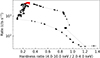 |
Fig. 1. HID of MAXI J1348–630 during its 2019 outburst. The intensity is the count rate in the 2–10 keV band, while the hardness ratio is the ratio of the count rate in the 4–10 keV band to that in the 2–4 keV band. Each point corresponds to one ExpID. The ExpIDs used in our work are marked in red. |
4.1. General GP fitting results
The DRW and SHO kernels, as well as their additive combinations with the AWN term, were tested against the X-ray data. The additive combination of SHO, DRW, and AWN is found to be the best model to characterize the variability features of the X-ray data. The AWN term is necessary, as adding it significantly reduces the AICc for small sample sizes (Akaike 1974; Burnham & Anderson 2004). For example, under the same GTI, the AICc values are 108 220 for the SHO and DRW, and 108 172 for the SHO, DRW, and AWN.
A difference of ΔAICc > 10 is generally taken as decisive evidence against the model with the higher AICc (Liddle 2007). For ΔAICc = 10, the Akaike weight (see Akaike 1981; Burnham & Anderson 2004) is w = e−10/2 ≈ 0.0067, meaning that the preferred model is 1/w ≈ 150 times better supported. Interpreted as a likelihood-ratio statistic, ΔAICc = 10 roughly corresponds to a 3σ significance level.
The final selected kernel function combines three key components, that is, SHO, DRW, and AWN. The SHO term serves as the primary tool for period detection, capturing the underlying oscillatory behavior in the data. The DRW componentmodels the stochastic background variability, accounting for correlated noise processes, along with its characteristic timescale. The AWN term handles another white noise component in the data in addition to the measurement uncertainties.
Figs. 2–4 show examples of the fitting results for the LE and HE data. The hardness ratio of the data we fit is concentrated around 0.3. The LE light curve has the highest mean count rate (approximately 4500 cts s−1), followed by HE (approximately 600 cts s−1), and ME shows the lowest value (approximately 200 cts s−1).
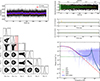 |
Fig. 2. LE fitting results when Q is free. Left column, from top to bottom: Light curve fitting results (including the mean prediction from the GP model and the 1σ uncertainty range corresponding to the total kernel) and parameter corner plot. Right column, from top to bottom: Residual distribution, ACF, and PSD. In PSD plot the blue line in the background represents the LSP, and the darker blue line is the total PSD of SHO (green line) and DRW (red line). The AWN term is plotted with the dotted purple line. |
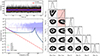 |
Fig. 4. HE fitting results when Q is free. Left column, from top to bottom: Light curve fitting results (including the mean prediction from the GP model and the 1σ uncertainty range corresponding to the total kernel) and PSD. Right column: Parameter corner plot. The ME fitting results are similar to the HE results, which are not shown. For both HE and ME, τDRW is not effectively constrained. |
In the fittings, we at first set the quality factor Q in the SHO kernel as a free parameter. This means that we did not have a prior belief about the QPO signature, although QPOs have been reported in the data through the frequency-domain method. Indeed, the median value of Q is restricted within the range of 5 − 10 by the data (Figs. 2 and 4), indicating that the SHO behaves as a good oscillator. The SHO PSD displays a clear peak at ω0/(2π)≈4.9 Hz. The fitting to the LE light curve yields τDRW ∼ 5 s. Looking at the DRW PSD, this characteristic timescale corresponds to the break frequency fb in the DRW PSD, given by τDRW = 1/(2πfb).
For each light curve, we find σn > σDRW. The LE data have the largest σn and σDRW among the LE, ME, and HE light curves, since the LE data have the highest count rate. The damping timescale in the DRW kernel is not constrained in the cases of the HE and ME observations (Fig. 4). This means that the stochastic variability is still correlated in the duration of the given GTI. The AWN power of the HE and ME data dominates over almost all effective frequencies. For the LE data, the DRW power exceeds the AWN power below ∼fb.
We again fit the same data with a fixed Q = 30 (the 1σ upper limit obtained above), which ensures a quasiperiodic component in the GP model and reduces the number of free parameters. The results are shown in Fig. 3. The fixed Q results in a significantly smaller S0, which arises from the intrinsic degeneracy between S0 and Q as discussed in Sect. 2. Given a fixed centroid frequency, a larger Q inherently corresponds to a smaller S0. The oscillation frequency and the parameters describing the background variability (DRW and AWN components) are nearly unchanged from a free Q to a fixed Q = 30. This means that the QPO can be modeled as a high-quality oscillation.
In the PSD plot, the blue line in the background represents the Lomb-Scargle periodogram (LSP), which is used as a supplementary method for comparison with the GP PSD. The LSP is a generalized form of the discrete Fourier power spectrum that is exactly equivalent to the least-squares fitting of a sinusoid at each trial frequency. Unlike the classical fast Fourier transform (FFT), the LSP is believed to remain statistically correct when the observations are uneven in time and when the data have point-by-point errors2 (VanderPlas 2018). Technically, the LSP PSD was obtained by directly applying the LombScargle function from the astropy package in Python. The GP approach offers a distinct advantage by decomposing the PSD into three physically interpretable components. This allows us to distinguish among the different physical processes contributing to the observed variability.
Figure 5 shows the representative PSDs3 calculated by GP and obtained using the powspec tool. Combining the GP results, we can now dive into the powspec PSD (frequency-domain method). The SHO component corresponds to the QPO signal (green peak in the right panel of Fig. 5). The DRW term matches the red line in the right panel of Fig. 5, both of which describe the PSD index variation in the low-frequency range. As mentioned above, the DRW component of the LE light curve is different from that of ME and HE light curves with a larger σDRW and a smaller τDRW, causing the DRW component to exceed the AWN component below ∼1/(2π τDRW) Hz. This also explains why the LE powspec PSD deviates from white noise below 1 Hz. We notice that τDRW is constrained within the range of [10 × tbinsize, 0.1 × tbaseline] by the LE data, where tbaseline is the duration of the given GTI. This indicates that τDRW is well constrained. The frequency-domain method reveals the presence of a second harmonic component at ∼9 Hz (Zhang et al. 2020a), which cannot be captured by the GP method.
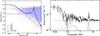 |
Fig. 5. PSD obtained using the GP method (left panel) and the PSD computed with powspec (right panel) for the same ExpID in the LE energy band. |
In GP method, the SHO term characterizes the QPO signal, and the rms of the SHO component is given by Eqs. (7) and (8), i.e.,  . The fractional rms of the SHO component is defined as
 (14)
(14)
The fractional rms of the SHO component for each GTI is derived from the GP fitting results, as shown in Fig. 6. The colors (purple, yellow, and red) correspond to the three discrete energy bands, with each line indicating the rms value for that GTI within the respective band. Specifically, the fractional rms obtained via the GP method ranges from 1.7 − 3.3% in the LE band (1–10 keV), increases to 7.5 − 13.6% in the ME band (10–30 keV), and then decreases to 4.2 − 9.9% in the HE band (30–100 keV). For comparison, the black lines in Fig. 6, with values of 2.7%, 13.3%, and 7.2% for the LE, ME, and HE bands, respectively, represent the fractional rms values calculated using the frequency-domain method for a representative ExpID4. These values lie within the corresponding fractional rms ranges inferred from the GP fits, indicating good consistency between the two approaches (Liu et al. 2022).
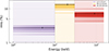 |
Fig. 6. Fractional rms of the three energy bands (LE, ME, and HE), calculated by dividing the standard deviation of the SHO term by the mean count rate. The colors (purple, yellow, and red) correspond to the three discrete energy bands, with each line indicating the rms value for that GTI within the respective band. The three black lines correspond to the fractional rms of a representative ExpID calculated using the frequency-domain method. |
4.2. Statistical analysis of the GP results
Based on the GP fitting results for the 362 GTIs, we performed a statistical analysis of the parameter values for the significant type-B QPO observations (204 GTIs). Figure 7 shows the evolution of the kernel parameters as a function of time and energy. The amplitude of the AWN term σn has larger uncertainties in some LE GTIs. This is because, on long time scales, the DRW component has a larger variance than the AWN term, which is clearly visible in the PSD plot. The values of σn obtained from the LE data are generally larger than those from the ME and HE bands. Meanwhile, the σn values in the ME and HE bands are also well constrained and show little temporal variation.
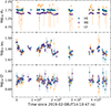 |
Fig. 7. Evolution of part of the parameters in the different energy bands with time when Q is free. From top to bottom: time evolution of σn, ω0, and Q. |
The natural oscillation frequency ω0 in the SHO kernel varies from 26 rad/s (4.1 Hz) to 31 rad/s (5.0 Hz) over time. The quality factor Q varies from 4 to 20. In general, ω0 and Q obtained from the ME data have the smallest uncertainties. Note that the ME light curve has the lowest count rate among the three energy bands and also the smallest well-constrained σn.
The relation between σn and ω0 is plotted in the upper panel of Fig. 8. There is a positive trend in the ME cases. However, the dynamic ranges of both variables are small. Consequently, we lack sufficient statistical confidence to confirm the validity of this trend. The lower panel of Fig. 8 illustrates the dependence of σn and τDRW of the LE band, since only the LE data have the well-constrained τDRW. The mean value of LE τDRW is 16 s, with a standard deviation of 1 s. The σn and the τDRW show no apparent correlation.
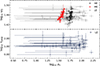 |
Fig. 8. Upper panel: relationship between parameters ω0 and σn in the different energy bands when Q is free. Lower panel: Relationship between parameters τDRW and σn in the LE band when Q is free. |
4.3. Key findings
Through GP modeling, we successfully decomposed the light curve of this source and identified its variability components. We also systematically compared their evolution across both energy and temporal domains. Our key findings are asfollows.
-
The stochastic variation component (DRW) of the LE band is markedly different from that of the ME and HE bands. In LE, correlations on the scale of τDRW were lost, whereas the data for ME and HE remain correlated on the timescale of the length of the light curve.
-
The SHO component behaves as a high-quality oscillator and does not exhibit obvious evolution in either the energy domain or the time domain, but the SHO component in the ME has the smallest uncertainty, which may be related to its smallest σn. Also, the ME data have the largest fractional rms, while the HE data show moderate values and the LE data the lowest.
-
An AWN term is needed, which implies that there is an extra uncorrelated (white noise) variation in the data.
These results contribute to a better understanding of the origins of the different components and their interactions.
5. Discussion
Using the GP method, we analyzed Insight-HXMT observations of MAXI J1348–630 during its type-B QPO phase. The GP method is a time-domain approach that models the light curve directly by superposing kernels, each with a specific mathematical form and physical interpretation. This is different from the frequency-domain method which typically fits the PSD with multiple Lorentziancomponents.
For MAXI J1348–630, during its type-B QPO phase, three distinct variability components are identified using the GP method: one quasiperiodic component (the SHO term) and two stochastic components (the DRW term and the AWN term). The SHO term corresponds to the Lorentzian feature that represents the QPO signal in the frequency domain. The DRW term captures the low-frequency red noise seen in the PSD, and the AWN term structurally represents an extra white noise component in the data. In frequency-domain analyses, such an extra white noise component has not received particular attention. However, in our case, we find that it dominates the data and likely carries important physical significance.
By leveraging the physical interpretability of GP kernels, we can explore the physical origins of the corresponding variability components. In the posterior distributions of the model parameters, the characteristic timescale τDRW shows distinct and intriguing behavior across the energy bands. Specifically, τDRW is well constrained in the LE band with typical values around ∼10 s, but is poorly constrained in both the ME and HE bands. The average lengths of the ME and HE GTI light curves are ∼400 s and ∼300 s, respectively. This lack of constraint on τDRW in ME and HE suggest that the physical relaxation timescales at higher energies are intrinsically longer than those at lowerenergies.
The distinct variation of τDRW across different energy bands are likely connected to the different physical origins of the X-ray photons. The LE photons primarily originate from the accretion disk, while the ME and HE photons are mainly produced through the inverse Compton scattering of disk photons in the corona. The DRW component could be associated with thermal instability in the accretion disk and the corona. The relaxation timescale was established by the balance of heating and cooling in the fluid. The shorter τDRW in the LE data implies that the thermal instability timescale in the accretion disk is shorter than that in the corona. The thermal instability timescale is given by tth ∼ (H/R)2 tvis, where tvis is the viscous timescale for the radial redistribution of mass and angular momentum, and H/R is the ratio between the scale height H and the radial extent R of the matter structure (Shakura & Sunyaev 1976). If we set tth ∼ τDRW ∼ 10 s, taking H/R ∼ 0.05, we obtain tvis ∼ 4000 s. This is reasonable for a stellar black hole system. In contrast, τDRW in the ME and HE bands cannot be well constrained by the current GTI light curves. This implies that the characteristic timescales in these bands are at least on the order of, or longer than, the duration of the GTIs, i.e., several hundred seconds or more. This is consistent with the expectation that the jet-like corona can extend up to hundreds of Rg during the type-B QPO phase (García et al. 2021).
Furthermore, the characteristic frequency of the DRW PSD is defined as fb = 1/(2π τDRW), indicating that a longer τDRW in the ME and HE bands corresponds to a lower characteristic frequency in these energy bands. This energy-dependent trend of fb is consistent with Insight-HXMT observations of MAXI J1820+070, where fb remains approximately constant at 0.1 Hz below 30 keV but decreases to below 0.04 Hz above 30 keV. Gao et al. (2025) attribute this behavior to the origin and scattering number of seed photons. Specifically, photons originating from the opposite side of the accretion disk traverse through the corona, undergoing multiple Compton upscatterings before reaching the observer. The number of scatterings is determined by the photons’ paths through the corona, and the emission direction tends to align with the photon’s incident direction into the corona when the optical depth exceeds 4 (Pozdnyakov et al. 1983). Lower-frequency photons originate from more distant disk regions, where photons undergo more scatterings in the corona, resulting in higher-energy emission and a lower characteristicfrequency.
For MAXI J1348–630, spectral-timing analysis suggests the presence of two distinct coronae (García et al. 2021; Zhang et al. 2022). The smaller corona is nearly spherical, with a characteristic size on the order of tens of Rg, while the larger corona exhibits a jet-like shape extending to scales of several hundred Rg, as inferred from the time-dependent vKompth model (García et al. 2021; Alabarta et al. 2025). Based on this geometry, we propose that seed photons with higher characteristic frequencies (fb) in the lower energy bands originate from regions closer to the black hole and are predominantly Comptonized in the spherical small corona, where the photon path lengths are relatively short. In contrast, seed photons with lower fb observed at higher energies likely arise from more distant regions of the disk and undergo Comptonization in the extended, jet-like corona, resulting in longer photon path lengths, particularly considering the low inclination ( ) of MAXI J1348–630 (Carotenuto et al. 2022). Moreover, the optical depth remains below 2 during the type-B QPO phase (García et al. 2021). This may indicate that the seed photons originate not only from the far side of the disk, as proposed for MAXI J1820+070, but potentially from the entire disk region.
Interestingly, an AWN component is needed to fit the LE, ME, and HE light curves. We could interpret this AWN component as a second DRW process with a characteristic timescale so short that it remains unresolved by our 0.03 s binning (e.g., Zhang et al. 2025b). We also attempted to use the light curve in a time bin of 0.01 s and replace the AWN term with a second DRW component to fit the data, but the short damping timescale is still not detected. This indicates that the second DRW component has a characteristic timescale of τDRW < 0.01 s.
Gao et al. (2025) reported the broadband PSD of the multiband X-ray data for MAXI J1820+070. Looking at their Fig. 2, we find that the broadband PSD (not including the QPO peak) can be described with a broken power-law:
 (15)
(15)
where αi is the PSD index and fb, i is the break frequency. For instance, the 1–10 keV PSD index of MAXI J1820+070 typically varies from α1 ≈ 0 to α2 ≈ 1 and then to α3 ≈ 2, with the two break frequencies being fb, 1 ∼ 0.06 Hz and fb, 2 ∼ 2 Hz. The two break frequencies reflect two timescales, given by 1/(2πfb), of 3 s and 0.08 s, respectively. The shorter timescale decreases to ∼0.02 s for the data above 76 keV. Such a broadband PSD has also been reported in other sources with fb, 2 ∼ 5 Hz, for example, XTE J1859+226 (Motta et al. 2022) and GX 339–4 (Zhang et al. 2023). For MAXI J1348–630, we identify two characteristic timescales: ∼10 s and < 0.01 s. The different physical timescales reflect distinct physical environments in these sources.
Physically, the ANW, that is, the rapid DRW variability with a damping timescale less than 0.01 s appearing in all the three energy bands, likely points to small-scale, high-frequency instabilities, most plausibly magnetorotational instability (MRI) operating in both the accretion disk and the corona. This suggests that their magnetic fields are dynamically coupled. Moreover, since σn > σDRW, the MRI-driven fluctuations exhibit a larger amplitude than the slower thermal instabilities.
We also detect a quasiperiodic signal (the SHO term) at similar frequencies (∼4.6 Hz) and comparable quality factors across all three energy bands. This common periodicity implies a shared driving mechanism and a similar emission-region structure across the disk and the corona. This also suggests that the disk and corona are coupled on a longer timescale of 2π/ω0 ≈ 0.2 s. This disk-corona oscillation could be driven by a relative large-scale modulation of the MRI.
Our analysis reveals a timescale hierarchy as follows: the AWN (rapid DRW) has the shortest timescale; followed by the SHO; then the disk DRW; and finally the corona DRW. The two shorter timescale terms, the AWN and the SHO, may arise from MRI turbulence and therefore appear in all three energy bands (LE, ME, and HE), linking the disk and corona through shared magnetic loops. The two longer DRW timescales possibly trace thermal-viscous relaxation: the smaller, well-resolved timescale in LE matches the thermal instability timescale of the thin, gas-pressure-dominated disk, whereas the currently unconstrained damping timescale in ME and HE points to a longer thermal instability timescale in the geometrically thick, Comptonizing corona. However, as shown in Fig. 8, the three processes (SHO, DRW, and AWN) appear to be independent and have no influence upon each other.
At present, the celerite framework is confined to the kernels that can be written as finite sums of exponentials. This restriction makes it difficult to capture subtle features in light curves, such as the variability whose PSD follows an f−1 index within a specific frequency band (e.g., Gao et al. 2025).
To reduce the size of a single file, an observation is artificially split into multiple segments, called “exposures”, which represent only a time segmentation within an observation, distinct from the traditional exposure concept of a camera or CCD imaging instrument.
See O’Sullivan & Aigrain (2024) for caveats when applying the LSP to unevenly sampled data.
The data used are from the LE band with the ExpID P021400201101.
The ExpID used is P021400201101.
Acknowledgments
The authors sincerely thank the referee for the helpful suggestions that have significantly improved the quality of our work. This work used data from the Insight-HXMT mission, a project, funded by the China National Space Administration and the Chinese Academy of Sciences. RM acknowledges support from the Royal Society Newton Funds. DY thanks the funding support from the National Natural Science Foundation of China (NSFC) under grant No. 12393852.
References
- Aigrain, S., & Foreman-Mackey, D. 2023, ARA&A, 61, 329 [NASA ADS] [CrossRef] [Google Scholar]
- Akaike, H. 1974, IEEE T. Automat. Contr., 19, 716 [CrossRef] [Google Scholar]
- Akaike, H. 1981, J. Econometrics, 16, 3 [Google Scholar]
- Al Yazeedi, A., Russell, D. M., Lewis, F., et al. 2019, ATel, 13188, 1 [Google Scholar]
- Alabarta, K., Méndez, M., García, F., et al. 2025, ApJ, 980, 251 [NASA ADS] [CrossRef] [Google Scholar]
- Alabarta, K., Méndez, M., García, F., et al. 2022, MNRAS, 514, 2839 [NASA ADS] [CrossRef] [Google Scholar]
- Bellavita, C., García, F., Méndez, M., & Karpouzas, K. 2022, MNRAS, 515, 2099 [NASA ADS] [CrossRef] [Google Scholar]
- Burke, C. J., Shen, Y., Blaes, O., et al. 2021, Sci, 373, 789 [Google Scholar]
- Burnham, K. P., & Anderson, D. R. 2004, Sociol. Method. Res., 33, 261 [Google Scholar]
- Cao, X., Jiang, W., Meng, B., et al. 2020, Sci. China Phys. Mech. Astron., 63, 249504 [NASA ADS] [CrossRef] [Google Scholar]
- Carotenuto, F., Corbel, S., Fender, R., Woudt, P., & Miller-Jones, J. 2020, ATel, 13467, 1 [Google Scholar]
- Carotenuto, F., Tetarenko, A. J., & Corbel, S. 2022, MNRAS, 511, 4826 [NASA ADS] [CrossRef] [Google Scholar]
- Casella, P., Belloni, T., & Stella, L. 2005, ApJ, 629, 403 [Google Scholar]
- Chen, Y., Cui, W., Li, W., et al. 2020, Sci. China Phys. Mech. Astron., 63, 249505 [NASA ADS] [CrossRef] [Google Scholar]
- Done, C., Gierliński, M., & Kubota, A. 2007, A&ARv, 15, 1 [Google Scholar]
- Esin, A. A., McClintock, J. E., & Narayan, R. 1997, ApJ, 489, 865 [NASA ADS] [CrossRef] [Google Scholar]
- Foreman-Mackey, D., Agol, E., Ambikasaran, S., & Angus, R. 2017, AJ, 154, 220 [Google Scholar]
- Gao, C., Yu, W., & Yan, Z. 2025, ApJ, 986, 226 [Google Scholar]
- García, F., Méndez, M., Karpouzas, K., et al. 2021, MNRAS, 501, 3173 [NASA ADS] [CrossRef] [Google Scholar]
- Gendreau, K. C., Arzoumanian, Z., Adkins, P. W., et al. 2016, in Space Telescopes and Instrumentation 2016: Ultraviolet to Gamma Ray, eds. J. W. A. den Herder, T. Takahashi, & M. Bautz, SPIE Conf. Ser., 9905, 99051H [NASA ADS] [CrossRef] [Google Scholar]
- Giannios, D., Kylafis, N. D., & Psaltis, D. 2004, A&A, 425, 163 [NASA ADS] [CrossRef] [EDP Sciences] [Google Scholar]
- Guan, J., Ma, R., Tao, L., et al. 2024, ApJ, 976, 61 [Google Scholar]
- Homan, J., & Belloni, T. 2005, Ap&SS, 300, 107 [Google Scholar]
- Homan, J., Wijnands, R., van der Klis, M., et al. 2001, ApJS, 132, 377 [NASA ADS] [CrossRef] [Google Scholar]
- Ingram, A. R., & Motta, S. E. 2019, Nat. Astron., 85, 101524P [Google Scholar]
- Jithesh, V., Misra, R., Maqbool, B., & Mall, G. 2021, MNRAS, 505, 713 [NASA ADS] [CrossRef] [Google Scholar]
- Kylafis, N. D., Papadakis, I. E., Reig, P., Giannios, D., & Pooley, G. G. 2008, A&A, 489, 481 [NASA ADS] [CrossRef] [EDP Sciences] [Google Scholar]
- Kylafis, N. D., Reig, P., & Papadakis, I. 2020, A&A, 640, L16 [NASA ADS] [CrossRef] [EDP Sciences] [Google Scholar]
- Lamer, G., Schwope, A. D., Predehl, P., et al. 2021, A&A, 647, A7 [NASA ADS] [CrossRef] [EDP Sciences] [Google Scholar]
- Lasota, J.-P. 2001, Nat. Astron., 45, 449 [Google Scholar]
- Lewin, W. H. G., & van der Klis, M. 2006, Compact Stellar X-ray Sources (Cambridge: Cambridge University Press) [Google Scholar]
- Lewin, W. H. G., van Paradijs, J., & van der Klis, M. 1988, Space Sci. Rev., 46, 273 [Google Scholar]
- Liddle, A. R. 2007, MNRAS, 377, L74 [NASA ADS] [Google Scholar]
- Liu, C., Zhang, Y., Li, X., et al. 2020, Sci. China Phys. Mech. Astron., 63, 249503 [NASA ADS] [CrossRef] [Google Scholar]
- Liu, H. X., Huang, Y., Bu, Q. C., et al. 2022, ApJ, 938, 108 [Google Scholar]
- Ma, R., Méndez, M., García, F., et al. 2023, MNRAS, 525, 854 [CrossRef] [Google Scholar]
- MacLeod, C. L., Ivezić, Ž., Kochanek, C. S., et al. 2010, ApJ, 721, 1014 [Google Scholar]
- Matsuoka, M., Kawasaki, K., Ueno, S., et al. 2009, PASJ, 61, 999 [Google Scholar]
- Mendez, M., & Van Der Klis, M. 1997, ApJ, 479, 926 [CrossRef] [Google Scholar]
- Miller, J. M., Homan, J., Steeghs, D., et al. 2006, ApJ, 653, 525 [NASA ADS] [CrossRef] [Google Scholar]
- Motch, C., Ricketts, M. J., Page, C. G., Ilovaisky, S. A., & Chevalier, C. 1983, A&A, 119, 171 [Google Scholar]
- Motta, S. E., Belloni, T., Stella, L., et al. 2022, MNRAS, 517, 1469 [NASA ADS] [CrossRef] [Google Scholar]
- O’Sullivan, N. K., & Aigrain, S. 2024, MNRAS, 531, 4181 [Google Scholar]
- Pirbhoy, S. F., Baglio, M. C., Russell, D. M., et al. 2020, ATel, 13451, 1 [NASA ADS] [Google Scholar]
- Pozdnyakov, L. A., Sobol, I. M., & Syunyaev, R. A. 1983, Astrophys. Space Phys. Res., 2, 189 [Google Scholar]
- Rasmussen, C. E., & Williams, C. K. I. 2006, Gaussian Processes for Machine Learning (Cambridge: MIT Press) [Google Scholar]
- Reis, R. C., Fabian, A. C., & Miller, J. M. 2010, MNRAS, 402, 836 [NASA ADS] [CrossRef] [Google Scholar]
- Remillard, R. A., Sobczak, G. J., Muno, M. P., & McClintock, J. E. 2002, ApJ, 564, 962 [NASA ADS] [CrossRef] [Google Scholar]
- Russell, D. M., Baglio, C. M., & Lewis, F. 2019, ATel, 12439, 1 [NASA ADS] [Google Scholar]
- Rybicki, G. B., & Press, W. H. 1992, ApJ, 398, 169 [CrossRef] [Google Scholar]
- Rybicki, G. B., & Press, W. H. 1995, Phys. Rev. Lett., 74, 1060 [NASA ADS] [CrossRef] [Google Scholar]
- Sanna, A., Uttley, P., Altamirano, D., et al. 2019, ATel, 12447, 1 [NASA ADS] [Google Scholar]
- Shakura, N. I., & Sunyaev, R. A. 1976, MNRAS, 175, 613 [NASA ADS] [CrossRef] [Google Scholar]
- Shimomukai, R., Negoro, H., Nakajima, M., et al. 2020, ATel, 13459, 1 [Google Scholar]
- Soleri, P., Belloni, T., & Casella, P. 2007, MNRAS, 383, 1089 [NASA ADS] [CrossRef] [Google Scholar]
- Stevens, A. L., & Uttley, P. 2016, MNRAS, 460, 2796 [NASA ADS] [CrossRef] [Google Scholar]
- Sugiura, N. 1978, Commun. Stat. A-Theor., 7, 13 [Google Scholar]
- Tanaka, Y., & Shibazaki, N. 1996, ARA&A, 34, 607 [NASA ADS] [CrossRef] [Google Scholar]
- Tang, R., Yan, D., Zhang, H., et al. 2024, ApJ, 971, 26 [Google Scholar]
- Uhlenbeck, G. E., & Ornstein, L. S. 1930, Phys. Rev., 36, 823 [NASA ADS] [CrossRef] [Google Scholar]
- van der Klis, M. 1989, ARA&A, 27, 517 [NASA ADS] [CrossRef] [Google Scholar]
- VanderPlas, J. T. 2018, ApJS, 236, 16 [Google Scholar]
- Wijnands, R., & van der Klis, M. 1999, ApJ, 514, 939 [NASA ADS] [CrossRef] [Google Scholar]
- Yatabe, F., Negoro, H., Nakajima, M., et al. 2019, ATel, 12425, 1 [NASA ADS] [Google Scholar]
- Zhang, H., Yan, D., Zhang, P., Yang, S., & Zhang, L. 2021, ApJ, 919, 58 [NASA ADS] [CrossRef] [Google Scholar]
- Zhang, H., Yan, D., & Zhang, L. 2022, ApJ, 930, 157 [Google Scholar]
- Zhang, H., Yan, D., & Zhang, L. 2023, ApJ, 944, 103 [Google Scholar]
- Zhang, H., Yan, D., Zhang, L., & Tang, N. 2025a, MNRAS, 537, 2380 [Google Scholar]
- Zhang, H., Yan, D., Zhang, L., & Tang, N. 2025b, ApJ, 988, 206 [Google Scholar]
- Zhang, H., Yan, D., Zhou, J., Zhang, L., & Tang, N. 2025c, MNRAS, 540, 3790 [Google Scholar]
- Zhang, L., Altamirano, D., Cúneo, V. A., et al. 2020a, MNRAS, 499, 851 [NASA ADS] [CrossRef] [Google Scholar]
- Zhang, L., Altamirano, D., Remillard, R., et al. 2020b, ATel, 13465, 1 [Google Scholar]
- Zhang, L., Altamirano, D., Uttley, P., et al. 2021, MNRAS, 505, 3823 [NASA ADS] [CrossRef] [Google Scholar]
- Zhang, S.-N., Li, T., Lu, F., et al. 2020, Sci. China Phys. Mech. Astron., 63, 249502 [NASA ADS] [CrossRef] [Google Scholar]
- Zhang, W., Tao, L., Soria, R., et al. 2022, ApJ, 927, 210 [NASA ADS] [CrossRef] [Google Scholar]
- Zhang, Y., Méndez, M., Motta, S. E., et al. 2023, MNRAS, 527, 5638 [CrossRef] [Google Scholar]
- Zu, Y., Kochanek, C. S., Kozłowski, S., & Udalski, A. 2013, ApJ, 765, 106 [NASA ADS] [CrossRef] [Google Scholar]
All Figures
|
Fig. 1. HID of MAXI J1348–630 during its 2019 outburst. The intensity is the count rate in the 2–10 keV band, while the hardness ratio is the ratio of the count rate in the 4–10 keV band to that in the 2–4 keV band. Each point corresponds to one ExpID. The ExpIDs used in our work are marked in red. |
| In the text | |
|
Fig. 2. LE fitting results when Q is free. Left column, from top to bottom: Light curve fitting results (including the mean prediction from the GP model and the 1σ uncertainty range corresponding to the total kernel) and parameter corner plot. Right column, from top to bottom: Residual distribution, ACF, and PSD. In PSD plot the blue line in the background represents the LSP, and the darker blue line is the total PSD of SHO (green line) and DRW (red line). The AWN term is plotted with the dotted purple line. |
| In the text | |
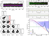 |
Fig. 3. Same as in Fig. 2 but Q is fixed at 30. |
| In the text | |
|
Fig. 4. HE fitting results when Q is free. Left column, from top to bottom: Light curve fitting results (including the mean prediction from the GP model and the 1σ uncertainty range corresponding to the total kernel) and PSD. Right column: Parameter corner plot. The ME fitting results are similar to the HE results, which are not shown. For both HE and ME, τDRW is not effectively constrained. |
| In the text | |
|
Fig. 5. PSD obtained using the GP method (left panel) and the PSD computed with powspec (right panel) for the same ExpID in the LE energy band. |
| In the text | |
|
Fig. 6. Fractional rms of the three energy bands (LE, ME, and HE), calculated by dividing the standard deviation of the SHO term by the mean count rate. The colors (purple, yellow, and red) correspond to the three discrete energy bands, with each line indicating the rms value for that GTI within the respective band. The three black lines correspond to the fractional rms of a representative ExpID calculated using the frequency-domain method. |
| In the text | |
|
Fig. 7. Evolution of part of the parameters in the different energy bands with time when Q is free. From top to bottom: time evolution of σn, ω0, and Q. |
| In the text | |
|
Fig. 8. Upper panel: relationship between parameters ω0 and σn in the different energy bands when Q is free. Lower panel: Relationship between parameters τDRW and σn in the LE band when Q is free. |
| In the text | |
Current usage metrics show cumulative count of Article Views (full-text article views including HTML views, PDF and ePub downloads, according to the available data) and Abstracts Views on Vision4Press platform.
Data correspond to usage on the plateform after 2015. The current usage metrics is available 48-96 hours after online publication and is updated daily on week days.
Initial download of the metrics may take a while.