© The Authors 2025

1 Introduction

Following the general observation that flat rotation curves are a common property of disk galaxies (e.g. Rubin et al. 1978, 1980; Bosma 1981), it has been suggested that this can be easily understood if the kinematical acceleration, a, and the gravitational acceleration, g, are identical in regions where the accelerations are above a common threshold, a₀, and the kinematical acceleration is proportional to the square root of the gravitational acceleration in low acceleration regimes (Milgrom 1983a,b,c). This scenario is expressed as $$a=g\mathrm{f}\mathrm{o}\mathrm{r}a\gg a_0\mathrm{a}\mathrm{n}\mathrm{d}a\propto \sqrt{g}\mathrm{f}\mathrm{o}\mathrm{r}a\ll a_0.$$(1)

This modification of Newtonian dynamics (MOND) immediately links the total baryonic mass of a galaxy, M_b, to the asymptotic flat rotation curve with velocity, v_∞, by $v_{\mathrm{\infty }}^4=a_{0}G{M}_{\mathrm{b}}$ (Milgrom 1983a), which has been observationally confirmed later to a high degree (McGaugh et al. 2000).

MOND field theories have been formulated as an extension of the Poisson equation. The AQUAL-formulation keeps the source term of the Poisson equation and replaces the Laplace operator by a non-linear operator in order to fulfil the boundary behaviour of the acceleration field in the Newtonian and MONDian regime (Bekenstein & Milgrom 1984). In a second widely used formulation (QUMOND), the Laplace operator of the Poisson equation is kept and the source term is replaced by a non-linear expression (Milgrom 2010).

The transition from the Newtonian to the MONDian regime is generally described by scaling the acceleration with a mapping where the argument is the ratio of the local kinematical or gravitational acceleration and a₀. However, there is no logical constraint for this transition function to be a function of a/a₀ only. The form of the transition can also depend, for example, on the local mass density and/or on the local symmetry of the mass distribution, indicating a dependence on ρ and ∇ρ. The only boundary conditions that MOND imposes are those in Eq. (1), as already pointed out by Bekenstein & Milgrom (1984). We note that MOND-type theories offer a valid description of gravity in the weak field limit, then small deviations from Newtonian gravity would already be expected on sub-Galactic scales (Milgrom 1983a,b,c). Open star clusters in the solar vicinity display asymmetric tidal tails (Jerabkova et al. 2021; Boffin et al. 2022), which are unlikely to form in Newtonian dynamics (Pflamm-Altenburg et al. 2023; Kroupa et al. 2024); however, they do appear in QUMOND dynamics (Kroupa et al. 2022) and Milgrom-law-dynamics (MLD) (Pflamm-Altenburg 2025). MONDian dynamics is expected to show observable differences to Newtonian dynamics in the orbital evolution of extreme trans-Neptunian objects (Paučo & Klacka 2016; Paučo 2017; Brown & Mathur 2023).

Blanchet & Novak (2011) quantified the additional quadrupole moment produced by MOND in the inner Solar System and concluded that the MOND interpolation function for the Solar System requires a very sharp transition in order be in agreement with orbital precession data of Jupiter. The requirement of a rapid transition from the Newtonian to the MONDian regime is also in line with the results from Cassini tracking data (Hees et al. 2014, 2016).

Hernandez et al. (2012) proposed that it could be valuable to analyse the kinematics of wide binaries as a critical test. Local binaries with a separation of more than ≈7000 AU are expected to be characterised by internal accelerations and relative velocities that are slightly higher than expected from Newtonian dynamics.

A number of later studies have reported a non-Newtonian dynamical behaviour of wide binaries (Hernandez et al. 2019, 2022; Hernandez 2023; Hernandez et al. 2024b; Chae 2023, 2024a,b), while others have found no deviations from Newtonian theoretical expectations (Pittordis & Sutherland 2023; Banik et al. 2024; Cookson 2024). However, Hernandez et al. (2024a) and Hernandez & Kroupa (2025) did report their discovery of critical problems in the statistical analysis of wide binaries in Pittordis & Sutherland (2023), Banik et al. (2024), and Cookson (2024).

In addition to the critiques mentioned above, the study performed by Banik et al. (2024) suffers from another problem. The orbital modelling of wide binaries in Banik et al. (2024) was done by replacing the two-body system by an effective one-body system, where the central mass is equal to the sum of both binary components and is orbited by a massless test particle (Banik et al. 2024, Sect. 3.1.1, 4th par.). These authors argued that in the inner region, the binaries follow Newtonian dynamics; whereas in the outer regions, the binaries follow an effective Newtonian dynamics, where the scaling factor is dominated by the higher external acceleration (called the external field effect, EFE). All wide binaries were treated as lying either in the Newtonian or the EFE-dominated regime and a linearity was applied between the mass distribution and the resulting gravitational fields.

Nonetheless, the FWHM of the mass distribution of the stellar masses of the wide binary sample was found to lie in the range from 0.4 to 1 M_⊙ (Banik et al. 2024, Fig. 5) and the vast majority of wide binaries have projected separations of 5000 AU and below (Banik et al. 2024, Fig. 6). At a 2000 AU distance from a 1 M_⊙ star, the internal Newtonian acceleration is 12.6 a₀ and at a 5000 AU distance, that is reduced to 2 a₀. For a 0.4 M_⊙ star, the acceleration is 5 a₀ at 2000 AU and 0.8 a₀ at 5000 AU. As their assumed external acceleration exerted by the Galactic gravitational field is about 1.14 a₀, most of the binaries are located in the non-linear transition regime from Newtonian to EFEMOND dynamics. Banik et al. (2024) claimed that the orbital evolution of wide binaries underlying MOND is excluded by a 16 σ confidence. However, Hernandez et al. (2024a) pointed out that the sample used in Banik et al. (2024) contains kinematic contaminants and that in the case of the binary subsample with a separation between 12 and 5 kAU their MOND models are closer to the observations than the Newton models (among other inconsistencies; see Sect. 3.2 in the cited paper). Furthermore, claiming the failure of MOND with a such high confidence requires a proper and very accurate orbit modelling procedure in MOND on the theoretical side. Therefore, the strong conclusion made by Banik et al. (2024) remains questionable.

The main motivation for the present work is to calculate complete solutions of the two-body problem in MONDian field theories and the comparison with the effective one-body problem. As a first step, the QUMOND formulation is considered on the basis of the linearity of the Laplace operator. In Sect. 2, an integral expression for the acceleration of a point mass in an N-body system is calculated using a Green’s integral representation of the solution of the linear QUMOND pde. In Sect. 4, we summarise the numerical routines used for the calculation of the integrals. In Sect. 5, Green’s integrals are calculated numerically for an isolated binary and compared with analytical expressions for the deep MOND case. The case of a collinear binary with a total mass of 2 M_⊙ embedded in an external Galactic field is considered in Sect. 6. In Sect. 7, we describe the three-dimensional (3D) analysis of this binary. In Sect. 8, we explore an embedded binary in Milgrom law dynamics (MLD) in brief, followed by a proposal of an alternative observational test in Sect. 9.

2 The particle acceleration of an N-body system in QUMOND

The QUMOND formulation was introduced by Milgrom (2010). The kinematical potential, Φ_Q, determines the acceleration field of a fluid via $$\mathbf{a}=-\mathrm{\nabla }{\mathrm{\Phi }}_{\mathrm{Q}},$$(2)

which is linked to a non-linear source, $$\mathrm{\Delta }{\mathrm{\Phi }}_{\mathrm{Q}}=\mathrm{\nabla }(\nu (|{\mathrm{\Phi }}_{\mathrm{N}}|/a_0)\mathrm{\nabla }{\mathrm{\Phi }}_{\mathrm{N}}),$$(3)

where Φ_N is the Newtonian potential and obtained from the standard Poisson equation, $$\mathrm{\Delta }{\mathrm{\Phi }}_{\mathrm{N}}=4\pi G\rho ,$$(4)

with the baryonic mass density, ρ.

The ν function joins the MONDian and the Newtonian regime continuously and is currently based on observations of rotation curves of disk galaxies. The choice of the transition function is restricted by the boundary conditions in Eq. (1), requiring $$\nu (y)=1\mathrm{f}\mathrm{o}\mathrm{r}y\gg 1\mathrm{a}\mathrm{n}\mathrm{d}\nu (y)=y^{-1/2}\mathrm{f}\mathrm{o}\mathrm{r}y\ll 1.$$(5)

The transition functions used in this work are summarised in Table 1. The threshold acceleration is set to a₀ = 1.2 × 10⁻¹⁰ m/s² (Begeman et al. 1991) corresponding to a₀ = 7.988 × 10⁻⁷ AU/yr⁻².

As already mentioned in Milgrom (2010) the solution of the kinematical potential is given by a Green’s integral expression with respect to an arbitrary but constant reference point, x₀, $$\begin{gathered} {\mathrm{\Phi }}_{\mathrm{Q}}(\mathbf{x}) \\ ={\int }_{{\mathbb{R}}^3}(G(\mathbf{x},\mathbf{y})-G({\mathbf{x}}_0,\mathbf{y}))\mathrm{\nabla }[\nu (|{\mathrm{\Phi }}_{\mathrm{N}}(\mathbf{y})|/a_0)\mathrm{\nabla }{\mathrm{\Phi }}_{\mathrm{N}}(\mathbf{y})]d^3\mathbf{y}, \end{gathered}$$(6)

where $$G(\mathbf{x},\mathbf{y})=-\frac{1}{4\pi |\mathbf{x}-\mathbf{y}|}$$(7)

is the Green’s function of the Laplace operator in the case of an unbounded domain.

A practical equivalent formulation to Eq. (3) can be written as $$\mathrm{\Delta }{\mathrm{\Phi }}_{\mathrm{Q}}=4\pi G(\rho +{\rho }_{\mathrm{p}\mathrm{d}\mathrm{m}}),$$(8)

where ρ_pdm is the so-called phantom dark matter $${\rho }_{\mathrm{p}\mathrm{d}\mathrm{m}}:=\frac{1}{4\pi G}\mathrm{\nabla }\left[(\nu (|\mathrm{\nabla }{\mathrm{\Phi }}_{\mathrm{N}}|/a_0)-1)\mathrm{\nabla }{\mathrm{\Phi }}_{\mathrm{N}}\right].$$(9)

The phantom dark matter can be interpreted as an additional, albeit non-existing matter distribution that causes the dynamical deviation of a system from an evolution in pure Newtonian dynamics.

The acceleration field at an arbitrary position, x, can be calculated from the gradient of the kinematical potential with $$\mathbf{a}(\mathbf{x})=-{\int }_{{\mathbb{R}}^3}\mathbf{G}(\mathbf{x},\mathbf{y})\mathrm{\nabla }[\nu (|{\mathrm{\Phi }}_{\mathrm{N}}(\mathbf{y})|/a_0)\mathrm{\nabla }{\mathrm{\Phi }}_{\mathrm{N}}(\mathbf{y})]d^3\mathbf{y},$$(10)

where G(x, y) is the gradient (with respect to x) of the Green’s function in Eq. (7) $$\mathbf{G}(\mathbf{x},\mathbf{y})=\frac{1}{4\pi }\frac{\mathbf{x}-\mathbf{y}}{|\mathbf{x}-\mathbf{y}{|}^3}.$$(11)

Applying the product rule to the divergence operator the integral for the acceleration can be split into two terms $$\begin{gathered} \mathbf{a}(\mathbf{x})=-{\int }_{{\mathbb{R}}^3}\mathbf{G}(\mathbf{x},\mathbf{y})\mathrm{\nabla }[\nu (|{\mathrm{\Phi }}_{\mathrm{N}}(\mathbf{y})|/a_0)]\bullet \mathrm{\nabla }{\mathrm{\Phi }}_{\mathrm{N}}(\mathbf{y})d^3\mathbf{y} \\ \phantom{\mathbf{a}(\mathbf{x})}-4\pi G{\int }_{{\mathbb{R}}^3}\mathbf{G}(\mathbf{x},\mathbf{y})\nu (|{\mathrm{\Phi }}_{\mathrm{N}}(\mathbf{y})|/a_0)\rho (\mathbf{y})d^3\mathbf{y}. \end{gathered}$$(12)

So far, the mass density distribution can be arbitrary.

Now, consider a system of n particles with masses (m₁,..., m_n) and position vectors (r₁|,..., r_n). The corresponding mass density distribution is $$\rho (\mathbf{y})=\sum _{i=1}^n{m}_i\delta (\mathbf{y}-{\mathbf{r}}_i).$$(13)

The Newtonian acceleration field at a position $\mathbf{x}\ne {\mathbf{r}}_i$ between the particles is given by $$\mathbf{g}(\mathbf{x})=-4\pi G{\int }_{{\mathbb{R}}^3}\mathbf{G}(\mathbf{x},\mathbf{y})\rho (\mathbf{y})d^3\mathbf{y}=-G\sum _{i=1}^n{m}_i\frac{\mathbf{x}-{\mathbf{r}}_i}{|\mathbf{x}-{\mathbf{r}}_i{|}^3}.$$(14)

The Newtonian acceleration of the particle j can be obtained by evaluating the integral for x = r_j, $$\begin{gathered} {\mathbf{g}}_j=-4\pi G{\int }_{{\mathbb{R}}^3}\mathbf{G}({\mathbf{r}}_j,\mathbf{y})\rho (\mathbf{y})d^3\mathbf{y} \\ =-G\sum _{i=1}^n{m}_i{\int }_{{\mathbb{R}}^3}\mathbf{G}({\mathbf{r}}_j,\mathbf{y})\delta (\mathbf{y}-{\mathbf{r}}_i)d^3\mathbf{y}. \end{gathered}$$(15)

Treating a point mass as the limit of a symmetric Dirac sequence, (δ_ε)_ε>0, with compact support identical to the ball with radius, ε, and centre, r_j, leads to $$\begin{gathered} {\mathbf{g}}_j=-G{m}_j\underset{\epsilon \to 0}{lim}{\int }_{{\mathbb{R}}^3}\mathbf{G}({\mathbf{r}}_j,\mathbf{y}){\delta }_{\epsilon }(\mathbf{y}-{\mathbf{r}}_j)d^3\mathbf{y} \\ -G\sum _{\begin{array}{c}i=1\\ i\ne j\end{array}}^n{m}_i\underset{\epsilon \to 0}{lim}{\int }_{{\mathbb{R}}^3}\mathbf{G}({\mathbf{r}}_j,\mathbf{y}){\delta }_{\epsilon }(\mathbf{y}-{\mathbf{r}}_i)d^3\mathbf{y}. \end{gathered}$$(16)

The integrand of the first term is antisymmetric with a symmetric support and vanishes for all values of ε. Thus, the self-contribution to the acceleration is 0. The integrand of the second term does not contain a singularity and therefore converges to the value of the Green’s function at the respective particle position. The Newtonian gradient of the whole (discontinuous) acceleration field is then given by the general expression $$\mathrm{\nabla }{\mathrm{\Phi }}_{\mathrm{N}}(\mathbf{x})=\{\begin{array}{ccc}\sum _{i=1}^{n}G{m}_i\frac{\mathbf{x}-{\mathbf{r}}_i}{|\mathbf{x}-{\mathbf{r}}_i{|}^3},& & \mathbf{x}\ne {\mathbf{r}}_j,\\ & & \\ \sum _{\begin{array}{c}i=1\\ i\ne j\end{array}}^{n}G{m}_i\frac{{\mathbf{r}}_j-{\mathbf{r}}_i}{|{\mathbf{r}}_j-{\mathbf{r}}_i{|}^3},& & \mathbf{x}={\mathbf{r}}_j.\end{array}$$(17)

To calculate the acceleration of the jth particle in QUMOND, we set x = r_j in Eq. (12). The delta distribution in the mass density of a particle system in Eq. (13) concentrates the contribution to the integral of the second term in Eq. (12) to the vicinity of the singularities, where the transition function tends to unity. Thus, the second term in Eq. (12) is identical to the Newtonian particle acceleration.

The QUMOND particle acceleration can then be expressed via $${\mathbf{a}}_j={\mathit{\alpha }}_j+{\mathbf{g}}_j,$$(18)

where α_j is the first term in Eq. (12).

Applying the chain rule to the ν-term in the integral for α_j, we obtain $${\mathit{\alpha }}_j=-\underset{{\mathbb{R}}^3}{\int }\mathbf{G}({\mathbf{r}}_j,\mathbf{y})\frac{{\nu }^{\mathrm{\prime }}(|\mathrm{\nabla }{\mathrm{\Phi }}_{\mathrm{N}}(\mathbf{y})|/a_0)}{|\mathrm{\nabla }{\mathrm{\Phi }}_{\mathrm{N}}(\mathbf{y})|a_0}\left(\mathrm{\nabla }{\mathrm{\Phi }}_{\mathrm{N}}\hat{\mathbf{T}}\right)(\mathbf{y})\bullet \mathrm{\nabla }{\mathrm{\Phi }}_{\mathrm{N}}(\mathbf{y})d^3\mathbf{y},$$(19)

where $${\left(\mathrm{\nabla }{\mathrm{\Phi }}_{\mathrm{N}}\hat{\mathbf{T}}\right)}_k(\mathbf{y}):=\sum _{l=1}^3{\left(\mathrm{\nabla }{\mathrm{\Phi }}_{\mathrm{N}}\right)}_l(\mathbf{y}){\hat{\mathbf{T}}}_{l,k}(\mathbf{y}),1\le k\le 3$$(20)

and $${\hat{\mathbf{T}}}_{l,k}(\mathbf{y})={\mathrm{\partial }}_l{\mathrm{\partial }}_k{\mathrm{\Phi }}_{\mathrm{N}}(\mathbf{y})=\sum _{i=1}^n\frac{G{m}_i}{|\mathbf{y}-{\mathbf{r}}_i{|}^3}({\delta }_{kl}-3\frac{(y_k-r_{i,k})(y_l-r_{i,l})}{|\mathbf{y}-{\mathbf{r}}_i{|}^2}),$$(21)

which is the symmetric 3 × 3 tidal tensor in the case of a Newtonian point mass system.

If the transition function tends to unity swiftly enough when approaching the particles, the integrand tends toward zero and the particles are surrounded by phantom dark-matter-free bubbles. Thus, the integral of the QUMOND contribution is free of any singularity and can be calculated conveniently.

The phantom dark matter density of an N-body system is given by $${\rho }_{\mathrm{p}\mathrm{d}\mathrm{m}}(\mathbf{y})=\frac{1}{4\pi G}\frac{{\nu }^{\mathrm{\prime }}(|\mathrm{\nabla }{\mathrm{\Phi }}_{\mathrm{N}}(\mathbf{y})|/a_0)}{|\mathrm{\nabla }{\mathrm{\Phi }}_{\mathrm{N}}(\mathbf{y})|a_0}\left(\mathrm{\nabla }{\mathrm{\Phi }}_{\mathrm{N}}\hat{\mathbf{T}}\right)(\mathbf{y})•\mathrm{\nabla }{\mathrm{\Phi }}_{\mathrm{N}}(\mathbf{y}).$$(22)

Thus, at large distances from a point mass or from the complete N-body system, the phantom dark matter density behaves as $${\rho }_{\mathrm{p}\mathrm{d}\mathrm{m}}(r)\approx \frac{1}{4\pi }\sqrt{\frac{a_{0}m}{G}}\frac{1}{r^2},$$(23)

where r is the distance to the point mass or the mass concentration.

One important point in Eq. (12) is that the second contribution is identical to the Newtonian acceleration only in the case of a point mass system. Now, we replace the point mass system by a smooth mass density distribution with identical total mass that is internally MONDian. In this case the ν-function in the second integral has a contribution to the integrand that is greater than unity. The integrand of the first integral contains Newtonian holes around each particle, if ν tends to one and its gradient tends to zero faster than the Newtonian gradient tends to infinity (depending on the choice of ν). It is not clear how a change in the mass distribution varies the values of the two integrals and whether or not the changes compensate each other. Here, the external field of the Galaxy is represented by a central massive third particle and not by a smooth external field.

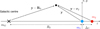Fig. 1 Set-up of particle positions.

3 Integrability of point mass systems

Even if the transition functions are continuous, there are three critical points where the integrability has to be checked. Figure 1 shows the general set up of the collinear particle system. The system is shifted so that the particle for which the QUMOND acceleration has to be calculated (as per Eq. (19)) is at the origin (unless stated otherwise). The other component of the binary is set on the positive z-axis with a separation of Δ_z to the first particle. In the case of an isolated binary, the point mass representing the Galaxy is omitted.

The distribution of the phantom dark matter along the connecting line (z-axis) of two particles with masses of m₁ = 1.8 M_⊙ and m₂ = 0.2 M_⊙ and a separation of Δz = 20 kAU can be seen in Fig. 2 for four different transition functions (Table 1). The maximum ν function indicates the transition from the Newtonian to the MONDian regions (|g_z| = a₀) at z = −9484AU, 9066AU, 17 243AU, 21 000AU. Outside the Newtonian region, the phantom dark matter density distributions of all four transition functions converge and scale with r⁻² (see Eq. (23)).

Between the two particles, a peak in the phantom dark matter density appears at z = 15 kAU indicating the location of zero-g, where the total Newtonian acceleration vanishes, independent of the choice of the transition function. In this context, it might be worthwhile to explore whether a real particle could indeed become trapped by this imaginary concentration of phantom dark matter. The appearance of MOND effects at the location of vanishing gravitational forces has already been mentioned by Hernandez (2017) in the context of mocking a central black hole in Globular clusters.

The jump of the phantom dark matter density in the case of the maximum transition function marks the positions where the local acceleration is identical to a₀. As the tidal tensor can be different at these positions, the phantom dark matter density can vary here as well.

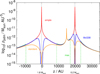Fig. 2 Phantom dark matter density distribution of an isolated two-body system.

3.1 Integrability for R → ∞

To obtain integrability for R → ∞, the composition (ν′ o |∇Φ_N|)(R) needs to scale with R^α with α ≤ 3. Since all transition functions, ν(y), scale with y⁻¹/² in the deep MOND regime, the composition scales with R³ and integrability is ensured for all transitions functions.

3.2 Integrability at zero-g points

We can consider a small ball with a radius, ε, centred on a zero-g point, where Green’s function has a nearly constant value. The Newtonian acceleration scales with ∇Φ_N ∝ ε in the direction of the z-axis. The whole integrand scales by ε^−1/2, which is compensated by ε² from the volume element. Thus, integrability is ensured for all transitions functions.

3.3 Integrability at particle locations

Next we consider a small ball with radius ε centred on a particle, where Green’s function scales with ε⁻² if the central particle is the specific particle whose acceleration is to be calculated and is constant in the case of any other particle. Thus, integrability needs to be checked only at the particle of interest. In this case, the composition (ν′ o |∇Φ_N|)(ε) needs to scale with ε^α with α ≥ 5. In the case of the standard integration function, the composition scales with ε⁶ and integrability is guaranteed.

In contrast, in the case of the simple transition function, the composition scales only with ε⁴ . Thus, the integral does not converge. This means, the simple transition function cannot be used in point mass descriptions in QUMOND. However, the integrand in Eq. (19) behaves in an antisymmetric manner in the vicinity of the particle (∝ ε⁻³). As the domain is symmetric, the antisymmetric parts cancel each other out if the integral is evaluated in the sense of the Cauchy principal value. The remaining symmetric part of the integrand is of the order of ∝ ε⁻² and integrable.

In the case of the McGaugh-transition function, the composition (ν′ o |∇Φ_N|)(ε) can be continued at ε = 0 by zero as C^∞. Since all the derivatives are equal to zero, it is not analytic and cannot be Taylor-expanded at ε = 0. Switching to spherical coordinates in the vicinity of the particle leads to an one-dimensional (1D) integral of a function proportional to $e^{1/\epsilon }/\left({\epsilon }^5{(e^{1/\epsilon }-1)}^2\right),$, which tends to 0 for ε → 0. Thus, integrability is ensured in this case.

4 Numerical integration

For simplicity, we focus in the first step on the embedded case, where both binary constituents and the Galaxy point mass are located on one line. Due to rotational symmetry around the z-axis, the dimension of the integral can be reduced to 2D after switching to polar coordinates and the calculations are reduced to the integration of the z-component based on a_x = a_y = 0.

In the case of an isolated binary, the integral with infinite domain is transformed to a finite domain by the mapping, $$\begin{gathered} \psi :[0,1[\times ]-1,1[\to {\mathbb{R}}_{\ge 0}\times \mathbb{R} \\ ({\xi }_r,{\xi }_z)\mapsto (\frac{\lambda {\xi }_r}{1-{\xi }_r},\frac{\lambda {\xi }_z}{1-{\xi }_z^2}), \end{gathered}$$(24)

where λ is a scaling parameter and set to λ = 2Δz in order to resolve the interior of the binary. The corresponding Jacobi determinant is $$|\mathrm{D}\psi (\mathit{\xi })|={\lambda }^2\frac{1}{(1-{\xi }_r{)}^2}\frac{1+{\xi }_z^2}{(1-{\xi }_z^2{)}^2}.$$(25)

In the case of a binary in the external field the domain of the integral is split into four subdomains with individual transformations:

i) $$\begin{gathered} {\psi }_1:[0,100\mathrm{\Delta }z]\times [-10\mathrm{\Delta }z,10\mathrm{\Delta }z]\to [0,100\mathrm{\Delta }z]\times [-10\mathrm{\Delta }z,10\mathrm{\Delta }z] \\ ({\xi }_r,{\xi }_z)\mapsto ({\xi }_r,{\xi }_z) \\ |\mathrm{D}{\psi }_1(\mathit{\xi })|=1, \end{gathered}$$(26)

ii) $$\begin{gathered} {\psi }_2:[0,1[\times [-10\mathrm{\Delta }z,10\mathrm{\Delta }z]\to [100\mathrm{\Delta }z,\mathrm{\infty }[\times [-10\mathrm{\Delta }z,10\mathrm{\Delta }z] \\ ({\xi }_r,{\xi }_z)\mapsto (100\mathrm{\Delta }z+{10}^7\frac{{\xi }_r}{1-{\xi }_r},{\xi }_z) \\ |\mathrm{D}{\psi }_2(\mathit{\xi })|={10}^7\frac{1}{{(1-{\xi }_r)}^2}, \end{gathered}$$(27)

iii) $$\begin{gathered} {\psi }_3:[0,1[\times [0,1[\to [0,\mathrm{\infty }[\times [10\mathrm{\Delta }z,\mathrm{\infty }[ \\ ({\xi }_r,{\xi }_z)\mapsto ({10}^7\frac{{\xi }_r}{1-{\xi }_r},10\mathrm{\Delta }z+{10}^7\frac{{\xi }_z}{1-{\xi }_z}) \\ |\mathrm{D}{\psi }_3(\mathit{\xi })|={10}^{14}\frac{1}{(1-{\xi }_r)(1-{\xi }_z)}, \end{gathered}$$(28)

iv) $$\begin{gathered} {\psi }_4:[0,1[\times ]-1,0]\to [0,\mathrm{\infty }[\times [-\mathrm{\infty },-10\mathrm{\Delta }z] \\ ({\xi }_r,{\xi }_z)\mapsto ({10}^7\frac{{\xi }_r}{1-{\xi }_r},-10\mathrm{\Delta }z+{10}^7\frac{{\xi }_z}{1+{\xi }_z}) \\ |\mathrm{D}{\psi }_4(\mathit{\xi })|={10}^{14}\frac{1}{(1-{\xi }_r)(1+{\xi }_z)}. \end{gathered}$$(29)

To explore the simple transition function, we refrained from the use of highly efficient adaptive cubature methods. Instead, we applied a 2D product rule of closed Newton-Cotes methods to an equidistant grid with incrementally decreasing bin size to force the symmetric evaluation of the integrand.

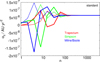Fig. 3 Speed of the convergence of the numerical integration of Eq. (19) for an equal-mass isolated binary and the standard transition function.

5 The QUMOND two-body system in isolation

5.1 Convergence of the integral

An equal-mass binary (m₁ = m₂ = 1 M_⊙) with a separation of Δz = 10 000 AU is calculated with the standard transition function. Because both masses are equal, they have identical accelerations except of the sign. Figure 3 shows the speed of the convergence of the absolute value of the acceleration as a function of the 1D cell number for the three simplest Newton-Cotes formulas. Particle one is located at the origin, r₁ = (0,0,0) (thin lines) and particle two is positioned on the positive z-axis, r₂ = (0,0, Δz) (thick lines). The accelerations converge to the same value.

In the case of the simple transition function, the numerical integration converges only for particle one, which is located at the origin. The basis points for the function evaluation are symmetrically distributed around the particle and the antisymmetric part of the integrand is compensated for independently. The symmetric part is absolutely integrable and the integration converges (Fig. 4, thin lines). In the case of particle two, the basis points of the integration routine are distributed asymmetrically around r₂ and the numerical integral does not converge (Fig. 4, thick lines).

5.2 Conservation of the linear momentum

It was shown in Milgrom (2010) that the total linear momentum is conserved in the QUMOND field formulation and the total force vanishes. As a test of the numerical scheme the z-component of the forces acting on each particle are calculated, $$F_{z,i}=m_i{a}_{z,i}=m_i(g_{z,i}+{\alpha }_{z,i}).$$

Their absolute values of a non-equal-mass binary (m₁ = 1.8 M_⊙, m₂ = 0.2 M_⊙, Δz = 10 000AU) are shown in Fig. 5 (solid lines) as a function of the cell number along one axis (simple transition function and symmetric evaluation). Indeed, the absolute values of the forces are identical. As the pure Newtonian part of the linear momentum is already conserved, the QUMOND part of the linear momentum fulfils an individual conservation law, $$0=\frac{d{p}_{\alpha ,z}}{dt}=m_1{\alpha }_{z,1}+m_2{\alpha }_{z,2}.$$(30)

The QUMOND part of the total force is shown in Fig. 5 (dashed lines).

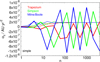Fig. 4 Speed of the (non)-convergence of the numerical integration of Eq. (19) for an equal-mass isolated binary and the simple transition function (symmetric evaluation for particle one, non-symmetric evaluation for particle two).

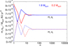Fig. 5 Forces of both components of a non-equal-mass isolated binary (simple transition function, symmetric evaluation).

5.3 Deep MOND limit

In the general, at the deep MOND limit, the force between two particles with masses m₁ and m₂ at a distance, z, can be calculated analytically (Milgrom 1994, 2014) via $$F_{2,1}=\frac{2\sqrt{G{a}_0}}{3z}((m_2+m_1{)}^{3/2}-m_1^{3/2}-m_2^{3/2}),$$(31)

after restricting the MOND field equation to the deep MOND limit.

Considering a point mass system in deep MOND requires two limiting operations: (i) ε (the radius of the symmetric domain of the Dirac sequence tends to zero; and (ii) The distance of the particles tends to infinity.

The general procedure is to first carry out the transition of the QUMOND field equation into the deep MOND regime and then to consider the point masses. This is in contrast to the procedure applied in this work: first, we considered the accelerations of a general N-body system. Then, in the second step, the particles were pushed apart from each other into the deep MOND regime. Thus, the limits were interchanged. The minimum requirement of interchanging limits is uniform convergence¹. Since the involved force laws (1/r and 1/r²) are non-uniformly continuous mappings, it is not clear how these procedures differ from each other.

During the transition of the QUMOND field equation into the deep MONDian regime, the Newtonian part is removed. In contrast, in the total acceleration in Eq. (18), the Newtonian term does not disappear when transiting into the deep MONDian regime. Thus, both procedures cannot be completely identical. However, this term becomes negligible.

Figure 6 shows the total force acting on the high-mass particle (m₁ = 1.8 M_⊙, m₂ = 0.2 M_⊙) as a function of the separation of the two particles from each other. The numerical results are marked by black solid circles. The analytical two-body force (Eq. (31)) is shown as the shallower solid blue line. The Newtonian force, F_N = Gm₁m₂/r² is indicated by the steeper red line.

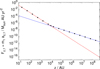Fig. 6 Total force acting on the high-mass particle as a function of the separation of the isolated binary described (simple transition function, symmetric evaluation).

5.4 Effective one-body system

From Eq. (31), we find that the relative acceleration of two particles with masses m₁ and m₂ is smaller than the acceleration of a massless test particle (m_tp = 0) in the field of a particle of combined mass m_tot = m₁ + m₂.

In the test particle system the acceleration of the central particle with m_tot ≠ 0 is $$\begin{array}{rl}{a}_{\mathrm{t}\mathrm{o}\mathrm{t}}=& \underset{m_2\to 0}{lim}\frac{F_{2,1}}{m_{\mathrm{t}\mathrm{o}\mathrm{t}}}\\ =& \underset{m_2\to 0}{lim}\frac{2\sqrt{G{a}_0}}{3z{m}_{\mathrm{t}\mathrm{o}\mathrm{t}}}(m_{\mathrm{t}\mathrm{o}\mathrm{t}}^{3/2}-(m_{\mathrm{t}\mathrm{o}\mathrm{t}}-m_2{)}^{3/2}-m_2^{3/2})=0.\end{array}$$(32)

The acceleration of the test particle can be calculated using L’Hôpital’s rule $$\begin{array}{rl}{a}_{\mathrm{t}\mathrm{p}}=& \underset{m_2\to 0}{lim}\frac{F_{2,1}}{m_2}\\ =& \underset{m_2\to 0}{lim}\frac{2\sqrt{G{a}_0}}{3z{m}_2}(m_{\mathrm{t}\mathrm{o}\mathrm{t}}^{3/2}-(m_{\mathrm{t}\mathrm{o}\mathrm{t}}-m_2{)}^{3/2}-m_2^{3/2})\\ =& \underset{m_2\to 0}{lim}\frac{\sqrt{G{a}_0}}{z}((m_{\mathrm{t}\mathrm{o}\mathrm{t}}-m_2{)}^{1/2}-m_2^{1/2})=\frac{\sqrt{G{a}_0}\sqrt{m_{\mathrm{t}\mathrm{o}\mathrm{t}}}}{z}.\end{array}$$(33)

Inserting the mass ratio q = m₂/m₁ with 0 ≤ q ≤ 1, the acceleration of the more massive particle is $$a_1=\frac{2\sqrt{G{a}_0{m}_{\mathrm{t}\mathrm{o}\mathrm{t}}}}{3z}\frac{(1+q{)}^{3/2}-1-q^{3/2}}{(1+q{)}^{1/2}},$$(34)

while that of the less massive particle $$a_2=\frac{2\sqrt{G{a}_0{m}_{\mathrm{t}\mathrm{o}\mathrm{t}}}}{3z}\frac{(1+q{)}^{3/2}-1-q^{3/2}}{q(1+q{)}^{1/2}}.$$(35)

The boost factor of the internal deep MOND acceleration of the effective test particle system with equal masses compared to the full two-body system is given by $$\frac{\mathrm{\Delta }{a}_{q=0}}{\mathrm{\Delta }{a}_q}=\frac{a_{\mathrm{t}\mathrm{o}\mathrm{t}}+a_{\mathrm{t}\mathrm{p}}}{a_{m_1}+a_{m_2}}=\frac{3q(1+q{)}^{1/2}}{2(1+q)((1+q{)}^{3/2}-1-q^{3/2})}.$$(36)

and depends only on the mass ratio. The boost factor as a function of q is shown in Fig. 7. The boost factor converges to 1 for q → 0 and has a maximum for q = 1 with a value of 3/(8 - √32) = 1.28....

Figure 8 shows the numerically calculated boost factors as a function of the separation of the two masses for different mass ratios as a function of the separation in the case of the standard transition function. In the Newtonian regime, the boost factor of the different configurations is 1, meaning that an isolated two-body system can be replaced by a test particle orbiting a central particle of combined mass as expected. In the deep MOND regime, the ratio of the acceleration converges very fast to a constant value following Eq. (36).

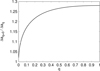Fig. 7 Boost factor of an equal-mass test particle system.

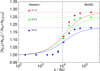Fig. 8 Boost factor of systems with constant total mass mtot = 2M⊙. The radial evolution is shown for three different systems: m1 = 1.0 M⊙, m2 = 1.0 M⊙ (red dots), m1 = 1.5 M⊙, m2 = 0.5 M⊙ (green dots), and m1 = 1.8 M⊙, m2 = 0.2 M⊙ (blue dots). The vertical dashed line marks the MOND radius $r_{\mathrm{M}}=\sqrt{G{m}_{\mathrm{t}\mathrm{o}\mathrm{t}}/a_0}$. The horizontal dashed lines mark the respective boost factor in the deep MOND limit according to Eq. (36). For comparison, the solid lines show the boost factor obtained from the analytical two-body force from (Zhao et al. 2010, their Eq. (A2)).

6 The collinear QUMOND two-body system in an external Galactic field

6.1 External field

The aim is to construct an external field as close as possible to the situation in Banik et al. (2024). In their effective one-body modelling procedure, the system is superimposed by a constant and homogenous Newtonian gravitational field. The field is calibrated to a circular rotation velocity of 232.8 km/s and a Galactocentric distance of R₀ = 8200 pc (McMillan 2017). These values determines the acceleration ratio a/a₀ = 1.785. Due to the problem of the replacement of a large number of particles by a smooth mass distribution (as outlined in the final paragraph of Sect. 2), the external field is realised by a central massive particle. Banik et al. (2024) used the simple transition function. In this case the ratio of the external Newtonian acceleration g_e and the threshold acceleration a₀ is g_e/a₀ = 1.144 and requires a central massive particle of $m_{\mathrm{G}}=R_0^2{g}_e/G=6.62\times {10}^{10}{M}_{\odot }$.

6.2 Distribution of the phantom dark matter

The distribution of the phantom dark matter density along the connecting line (z-axis) of two particles with masses m₁ = 1.8 M_⊙ and m₂ = 0.2 M_⊙ and a separation of Δ_z = 20 kAU can be seen in Fig. 9 for four different transition functions (Table 1) and both arrangements. The Galactic point mass is put at z = −8.2 kpc. Now, the location of the Galactic zero-g point between both binary components depends on the order and there appears a second zero-g point between the Galactic centre and the binary. A massless test particle does not produce a phantom dark matter peak between itself and any other real particle.

6.3 MONDian Path of a Newtonian binary

The Newtonian external acceleration at the location of the binary is g_e = 9.138 × 10⁻⁷ AU/yr². This corresponds to a kinematical acceleration of 1.426 × 10⁻⁶ AU/yr² (simple transition function).

Keeping the Newtonian acceleration constant and varying the transition function, the corresponding kinematical accelerations are then 1.122 × 10⁻⁶ AU/yr² (standard transition function) and 1.391 × 10⁻⁶ AU/yr² (McG08 transition function). The acceleration of the centre of mass of the binary is calculated via $$a_{z,com}=\frac{1}{m_1+m_2}(m_1(g_{z,1}+{\alpha }_{z,1})+m_2(g_{z,2}+{\alpha }_{z,2})).$$(37)

Figure 10 shows the numerically obtained acceleration values of the centre of mass of the equal-mass binary (m₁ = m₂ = 1 M_⊙) and of the effective single-body problems (m₁ = 2 M_⊙, m₂ = 0) compared to the external Newtonian acceleration scaled by the boost factors of the different transition functions. It can be seen that the centre of masses of the binaries move on a MONDian binary whether or not the binary is internally MONDian or Newtonian.

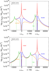Fig. 9 Phantom dark matter distribution of an two-body system in the Galactic EFE.

6.4 Effective one-body system versus the two-body system

Figure 11 shows the ratio of the internal relative kinematical acceleration to the internal relative Newtonian acceleration, $$\frac{\mathrm{\Delta }a}{\mathrm{\Delta }g}=\frac{|a_{z,2}-a_{z,1}|}{|g_{z,2}-g_{z,1}|},$$(38)

as a function of the internal separation for the equal-mass two-body system and for the effective one-body system. In the Newtonian regime, ≲10 kAU, the boost factor of the equal-mass binary increases at a rate that is slower (in line with the increasing separation) than the boost factor of both effective one-body systems in the case of the simple transition function with symmetric evaluation. The one-body system with the test particle between the Galactic centre and the massive binary component shows the fastest increase in the boost factor, lasting until the massless test particle reaches the Galactic zero g position, where both accelerations induced by the Galactic centre particle and the massive binary particle balance each other out ($\mathrm{\Delta }z=\sqrt{m_2/m_{\mathrm{g}\mathrm{a}\mathrm{l}}}{R}_0=9293.6\mathrm{A}\mathrm{U}$). Here, the boost factor drops abruptly and shows the slowest increase in the boost factor in the EFEregime. For large separations, the boost factor of the equal-mass binary converges against the theoretically expected maximum boost in the EFE-effect (η_max = ν_simp(g_ext/a₀) = 1.56 ). For the purposes of comparison with the work of Banik et al. (2024), the azimuthally averaged boost factor (their Figure 7) is superimposed scaled to a MOND radius of $r_{\mathrm{M}}=\sqrt{G2M_{\odot }/a0}=\mathrm{10\hspace{0.17em}038}\mathrm{A}\mathrm{U}$.

The unexpected behaviour of the massless test particle is due to the additional influence of the phantom dark matter spike produced by the Galactic zero-g point between the Galactic centre particle and the massive binary component. When the test particle recedes from the massive component approaching the phantom dark matter spike, it is subject to an increasing additional attraction towards the Galactic centre; thus, the difference in the kinematical acceleration increases. Once the test particle has passed the zero-g point, the additional attraction has switched the direction and leads to a fast decrease of the difference of the accelerations.

The differences in the boost factors in the case of the standard transition function is shown in Fig. 12 and in the case of the McG08 transition function, these data are given in Fig. 13. All three models have in common that within the MOND radius the effective one-body systems have higher boost factors than the equal-mass system.

The boost factor in the transition regime is shown in Fig. 14 for different mass ratios. The equal-mass binary has got the lowest boost factor. And for all these cases, configurations where the lower-mass component is located between the Galactic centre and the higher-mass component display higher internal relative accelerations than in cases of the opposite mass ordering.

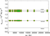Fig. 10 Centre of mass accelerations as a function of the internal separation. Red circles: particle order of mgal−2 M⊙−0 M⊙. Green squares: particle order of mgal−1 M⊙−1 M⊙. Black triangles: particle order of mgal−0 M⊙−2 M⊙. Equal-mass binary is Newtonian for Δz = √2M⊙ G/a0 ≤ 10 038 AU.

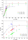Fig. 11 MOND boost factor of the internal relative acceleration in the case of the simple transition function. The horizontal solid line in the upper diagram shows the maximum boost ηmax = 1.56. The vertical solid line marks the zero-g distance of a massless test particle. The short dashed line shows the azimuthally averaged boost factor from Banik et al. (2024). The bottom diagram shows a zoom-in of the upper diagram in the transition region.

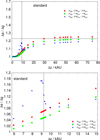Fig. 12 MOND boost factor of the internal relative acceleration in the case of the standard transition function. The horizontal line in the upper diagram shows the maximum boost ηmax = 1.23. The vertical line marks the zero g distance of a massless test particle. The bottom diagram shows a zoom-in of the upper diagram in the transition region.

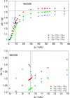Fig. 13 MOND boost factor of the internal relative acceleration in the case of the McG08 transition function. The horizontal line in the upper diagram shows the maximum boost ηmax = 1.52. The vertical line marks the zero g distance of a massless test particle. The bottom diagram shows a zoom-in of the upper diagram in the transition region.

7 Embedded binary in three dimensions

In this section, the embedded equal-mass binary and the corresponding effective one-body system are considered in a 3D configuration for the cases of a separation of Δz = 9000 AU, where the discrepancy in the relative acceleration is greatest, and a separation of Δz = 75 000 AU, where the binary is in the deep EFE. The McG08-transition function is used for these calculations. Here, the integral in Eq. (19) is evaluated in three dimensions. The partitioning of the domain has been adjusted.

The mass of the first particle is kept at the origin (m₁ = 2 M_⊙ in case of the effective one-body system). The second mass is rotated with a constant distance to the first particle in steps of Δϑ = 1° in the x - z-plane (x₂ = Δz sin(ϑ), y₂ = 0, z₂ = ∆z cos(ϑ)). In the case of the effective binary ϑ = 0 corresponds to the collinear ordering m_gal - 2 M_⊙ - 0 M_⊙ and ft = 180° corresponds to the collinear ordering m_gal - 0 M_⊙ - 2 M_⊙ discussed in the previous section.

Figure 15 shows the boost factor |a₂ - a₁|/|g₂ - g₁| as a function of the inclination angle ft. In the case of the equal-mass binary the boost factor is maximal for the perpendicular configuration and has a minimum for the collinear setting. In the case of the effective binary, the boost factor has a minimum for the configuration where the test particle is at the outer most position and increases continuously with increasing inclination. Interestingly, the maximum is not reach at the position where the test particle is between the mass particle and the Galactic centre but close to it. This might be due to the axis-symmetry of the distribution of the phantom dark matter. If the test particle is positioned on the z-axis, a higher fraction of the acceleration is cancelled out than if the test particle is slightly displaced from the z-axis. Figure 16 shows different directions of the QUMOND contribution to the kinematical acceleration.

The boost factor for a separation of 75 000 AU is shown in Fig. 17. In the deep EFE, the relative acceleration is lowest for the perpendicular orientation and highest for the collinear configuration. The directions of the QUMOND contributions are displayed in Fig. 18.

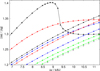Fig. 14 Mass dependence of the boost factor. Shown is the boost factor of the collinear configuration of a binary with a total mass of 2 M⊙ with different mass ratios as a function of the internal separation: 2.0-0.0 M⊙ (black), 1.5-0.5 M⊙ (green), 1.9-0.1 M⊙ (blue), and 1.99-0.01 M⊙ (red). The equal-mass binary is plotted with grey squares. The configurations with the less massive component between the higher-mass component and the Galactic centre particle are indicated by triangles, while those where the less-mass component is on the side of the Galactic anti-centre are indicated by circles.

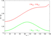Fig. 15 3D boost factor for Δz = 9000 AU. Ratios of the absolute values of the total kinematical and the Newtonian acceleration are shown as a function of the inclination angle for the equal-mass binary and the effective one-body system.

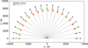Fig. 16 Directions of QUMOND contributions for Δz=9000 AU. Green arrows indicate the direction of the QUMOND contribution to the acceleration in the case of the equal-mass binary. Red arrows indicate the direction of the QUMOND contribution to the acceleration in the case of the effective one-body system. The lengths of the arrows scale linearly with the absolute value of the QUMOND contribution.

Fig. 17 3D boost factor for Δz = 75 000 AU. Details are similar to Fig. 15.

8 Wide binaries in Milgrom law dynamics (MLD)

A different MOND formulation we followed as part of this study is MLD, with the aim to explore the boost factors of the internal binary dynamics. In MLD, the relation between the radial kinematical acceleration, a_r, and the radial Newtonian gravitational acceleration, g_r, proposed by Milgrom (1983c) for disk galaxies has been postulated to be valid in vectorial form (Pflamm-Altenburg 2025). Although it allows for an easy and fast calculation of MONDian accelerations in N-body systems, this MOND formulation is incomplete. The disadvantage of this formulation is, that an internally Newtonian binary follows the external Newtonian path, rather than the MONDian orbit. To suppress the Newtonisation of compact subsystems, the Newtonian gravitational force has been softened with a smoothing parameter of 0.001 pc, which allows us to cover the full internal MONDian regime of wide binaries and open star clusters. It was demonstrated in the work of Pflamm-Altenburg (2025) that in contrast to previous statements (Felten 1984), an isolated MONDian two-body system does not show a general self-acceleration in the meaning of getting continuously faster. The constant and uniform motion of the Newtonian centre of mass is replaced by a constant and uniform motion of the MONDian centre of mass.

In MLD, the kinematical acceleration along the z-axis of particle i is $$a_i=\nu (|g_i+g_e|/a_0)(g_i+g_e),$$(39)

where the external acceleration is assumed to be homogeneous and g_i is the Newtonian acceleration exerted by the other binary component. In a simple estimate, we might argue that for large internal separations, the ν-factor is dominated by the external field (ν(g_e/a₀)) and the boost factor is $$\frac{\mathrm{\Delta }a}{\mathrm{\Delta }g}=\frac{|a_2-a_1|}{|g_2-g_1|}=\nu (g_e/a_0)\frac{|g_2-g_1|}{|g_2-g_1|}=\nu (g_e/a_0)>1.$$(40)

Taking the same external Newtonian acceleration as in the previous section, this boost factor is ν_simple(9.138 × 10⁻⁷ AU yr⁻²/a₀) = 1.56 in the case of the simple transition function. Figure 19 shows the numerical evaluation of the boost factor in MLD as a function of the internal separation and is much below the estimated value of 1.56.

Expanding the transition function into a Taylor series an analysis of the limit leads to the correct boost factor of $$\underset{\mathrm{\Delta }z\to \mathrm{\infty }}{lim}\frac{|a_2-a_1|}{|g_2-g_1|}=\nu (g_e/a_0)+{\nu }^{\mathrm{\prime }}(g_e/a_0)g_e/a_0.$$(41)

For the simple transition function, the true boost factor is 1.15, as can be seen in Fig. 19. In contrast to the QUMOND formulation, the boost factor of the equal-mass binary lies between both effective one body systems.

Each transition function is characterised by values greater than one and a negative derivative. Thus, boost factors smaller than one are possible in MLD. For the standard transition function, the wrong boost factor is 1.23 and the correct one is 0.92 (Fig. 20). MLD allows for a reduction in the internal dynamics, depending on the transition function and the strength of the external field.

Fig. 18 Directions of QUMOND contributions for Δz=75 000 AU. Details are similar to Fig. 16.

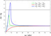Fig. 19 Boost factor in MLD with simple transition function. The solid horizontal line shows the wrong boost factor (Eq. (40)). The short dashed horizontal line shows the correct boost factor (Eq. (41)).

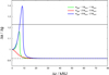Fig. 20 Boost factor in MLD with a standard transition function.

9 Proposal of an observational test

All tests on wide binaries compare the set of observed data pairs of the projected relative velocity with the projected separation of both constituents with those obtained from Newtonian and non-Newtonian modelling of wide binary populations. The detailed modelling of an ensemble of binaries require (in addition to the gravitational theory) assumptions on the distribution of structural parameters such as for example the mass ratio, the eccentricity and the semi major axis. However, a fundamental difference between Newtonian and MONDian binaries is that the relative acceleration between both constituents depends in MOND on the inclination angle of both stars in the case they have non-equal masses. The relative velocity between both stars should have an asymmetrical dependence on the position angle of the binary on sky with respect to the direction of the external field. This means it depends on whether or not the more massive component is closer to the Galactic centre (Fig. 21).

However, given the present line-of-sight errors, the 3D resolution of the binary configurations is too poor and such an observational test is currently not feasible. An observational detection of the effect is even more complicated, as demonstrated in the previous section. This is because the difference in the accelerations are only obvious for high mass ratios, which are atypical for stellar binaries.

However, the asymmetry in the acceleration and velocity field should exist in the Solar System as well. Thus, Oort-cloud and trans-Neptunian objects are also candidates to search for non-Newtonian asymmetries as they tend to have very high mass ratios with respect to the sun. Despite the current observational impossibility, it is worthwhile to work out detailed predictions in QUMOND dynamics and other MOND formulations.

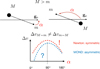Fig. 21 Expected asymmetry of relative velocities.

10 Summary and conclusions

In this work, we have constructed a method to obtain the acceleration of particles in an N-body system in QUMOND, which is consistent with the field formulation of QUMOND. The acceleration of a point mass is expressed via a Green’s integral, obtained by treating point masses as limits of Dirac sequences just as the Newtonian acceleration of a point mass is obtained from the Poisson equation. All QUMOND-transition functions ensure integrability at infinity and at zero-g points. At the particle singularity, the simple transition function is not absolutely integrable; whereas the McGaugh and the standard transition function indeed are.

This method was first applied to an isolated binary and compared to analytical solutions in the deep MOND limit. In the second step, we explore a wide binary embedded in an external Galactic field similar to the solar vicinity. If a binary is approximated by an effective one-body system where the central particle contains the total system mass and is orbited by a massless test particle, then the relative acceleration will be higher than in the full two-body system in the transition regime.

This has an important consequence for the results in Banik et al. (2024). As the vast majority of the binaries lie in the transition regime, the obtained accelerations in their modelling are higher than in the correct handling of binaries in QUMOND. Thus, testing binary dynamics in QUMOND against observational data requires the development of proper and consistent QUMOND-N-body orbit integrators. However, to speed up the calculations to a tolerable level calls for the 3D tensor-product integration methods to be replaced with an efficient non-tensortype integration algorithm, which would also include an suitable adaptive subpartitioning scheme. This would allow us to resolve the particle singularities and the phantom dark matter spikes at the Galactic zero-g points.

An additional zero-g point between both binary components appears. As these zero-g points show a local peak of phantom dark matter, it is worth exploring whether baryonic matter can be trapped and whether it is, in principle, detectable in the Solar System.

In this first step, the collinearly embedded binary is considered because the numerical integration is simplified thanks to a reduction of the integration from three to two dimensions. It is now straightforward to extend the numerical integration to three dimensions and to reinvestigate the orbit of Saturn in the context of the Cassini ranging data (Blanchet & Novak 2011; Hees et al. 2014, 2016) in more detail, along with the effective planet nine hypothesis (Paučo & Klacka 2016; Paučo 2017; Brown & Mathur 2023) and the wide-binary orbit modelling.

Simultaneously to the investigation of QUMOND N-body systems, it would also be useful to construct expressions for particle accelerations in N-body systems that are fully consistent with the field formulation of AQUAL. However, early considerations show that this approach would involve a numerical solution of 3D non-linear Fredholm integral equations of second kind.

References

All Tables

All Figures

	Fig. 1 Set-up of particle positions.
In the text

	Fig. 2 Phantom dark matter density distribution of an isolated two-body system.
In the text

	Fig. 3 Speed of the convergence of the numerical integration of Eq. (19) for an equal-mass isolated binary and the standard transition function.
In the text

	Fig. 4 Speed of the (non)-convergence of the numerical integration of Eq. (19) for an equal-mass isolated binary and the simple transition function (symmetric evaluation for particle one, non-symmetric evaluation for particle two).
In the text

	Fig. 5 Forces of both components of a non-equal-mass isolated binary (simple transition function, symmetric evaluation).
In the text

	Fig. 6 Total force acting on the high-mass particle as a function of the separation of the isolated binary described (simple transition function, symmetric evaluation).
In the text

	Fig. 7 Boost factor of an equal-mass test particle system.
In the text

Fig. 8 Boost factor of systems with constant total mass mtot = 2M⊙. The radial evolution is shown for three different systems: m1 = 1.0 M⊙, m2 = 1.0 M⊙ (red dots), m1 = 1.5 M⊙, m2 = 0.5 M⊙ (green dots), and m1 = 1.8 M⊙, m2 = 0.2 M⊙ (blue dots). The vertical dashed line marks the MOND radius $r_{\mathrm{M}}=\sqrt{G{m}_{\mathrm{t}\mathrm{o}\mathrm{t}}/a_0}$. The horizontal dashed lines mark the respective boost factor in the deep MOND limit according to Eq. (36). For comparison, the solid lines show the boost factor obtained from the analytical two-body force from (Zhao et al. 2010, their Eq. (A2)).

In the text

	Fig. 9 Phantom dark matter distribution of an two-body system in the Galactic EFE.
In the text

	Fig. 10 Centre of mass accelerations as a function of the internal separation. Red circles: particle order of mgal−2 M⊙−0 M⊙. Green squares: particle order of mgal−1 M⊙−1 M⊙. Black triangles: particle order of mgal−0 M⊙−2 M⊙. Equal-mass binary is Newtonian for Δz = √2M⊙ G/a0 ≤ 10 038 AU.
In the text

Fig. 11 MOND boost factor of the internal relative acceleration in the case of the simple transition function. The horizontal solid line in the upper diagram shows the maximum boost ηmax = 1.56. The vertical solid line marks the zero-g distance of a massless test particle. The short dashed line shows the azimuthally averaged boost factor from Banik et al. (2024). The bottom diagram shows a zoom-in of the upper diagram in the transition region.

In the text

	Fig. 12 MOND boost factor of the internal relative acceleration in the case of the standard transition function. The horizontal line in the upper diagram shows the maximum boost ηmax = 1.23. The vertical line marks the zero g distance of a massless test particle. The bottom diagram shows a zoom-in of the upper diagram in the transition region.
In the text

	Fig. 13 MOND boost factor of the internal relative acceleration in the case of the McG08 transition function. The horizontal line in the upper diagram shows the maximum boost ηmax = 1.52. The vertical line marks the zero g distance of a massless test particle. The bottom diagram shows a zoom-in of the upper diagram in the transition region.
In the text

Fig. 14 Mass dependence of the boost factor. Shown is the boost factor of the collinear configuration of a binary with a total mass of 2 M⊙ with different mass ratios as a function of the internal separation: 2.0-0.0 M⊙ (black), 1.5-0.5 M⊙ (green), 1.9-0.1 M⊙ (blue), and 1.99-0.01 M⊙ (red). The equal-mass binary is plotted with grey squares. The configurations with the less massive component between the higher-mass component and the Galactic centre particle are indicated by triangles, while those where the less-mass component is on the side of the Galactic anti-centre are indicated by circles.

In the text

	Fig. 15 3D boost factor for Δz = 9000 AU. Ratios of the absolute values of the total kinematical and the Newtonian acceleration are shown as a function of the inclination angle for the equal-mass binary and the effective one-body system.
In the text

	Fig. 16 Directions of QUMOND contributions for Δz=9000 AU. Green arrows indicate the direction of the QUMOND contribution to the acceleration in the case of the equal-mass binary. Red arrows indicate the direction of the QUMOND contribution to the acceleration in the case of the effective one-body system. The lengths of the arrows scale linearly with the absolute value of the QUMOND contribution.
In the text

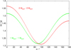	Fig. 17 3D boost factor for Δz = 75 000 AU. Details are similar to Fig. 15.
In the text

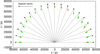	Fig. 18 Directions of QUMOND contributions for Δz=75 000 AU. Details are similar to Fig. 16.
In the text

	Fig. 19 Boost factor in MLD with simple transition function. The solid horizontal line shows the wrong boost factor (Eq. (40)). The short dashed horizontal line shows the correct boost factor (Eq. (41)).
In the text

	Fig. 20 Boost factor in MLD with a standard transition function.
In the text

	Fig. 21 Expected asymmetry of relative velocities.
In the text

References

- Banik, I., Pittordis, C., Sutherland, W., et al. 2024, MNRAS, 527, 4573 [Google Scholar]
- Begeman, K. G., Broeils, A. H., & Sanders, R. H. 1991, MNRAS, 249, 523 [Google Scholar]
- Bekenstein, J., & Milgrom, M. 1984, ApJ, 286, 7 [NASA ADS] [CrossRef] [Google Scholar]
- Blanchet, L., & Novak, J. 2011, MNRAS, 412, 2530 [CrossRef] [Google Scholar]
- Boffin, H. M. J., Jerabkova, T., Beccari, G., & Wang, L. 2022, MNRAS, 514, 3579 [NASA ADS] [CrossRef] [Google Scholar]
- Bosma, A. 1981, AJ, 86, 1825 [NASA ADS] [CrossRef] [Google Scholar]
- Brown, K., & Mathur, H. 2023, AJ, 166, 168 [Google Scholar]
- Chae, K.-H. 2023, ApJ, 952, 128 [NASA ADS] [CrossRef] [Google Scholar]
- Chae, K.-H. 2024a, ApJ, 972, 186 [Google Scholar]
- Chae, K.-H. 2024b, ApJ, 960, 114 [NASA ADS] [CrossRef] [Google Scholar]
- Cookson, S. A. 2024, MNRAS, 533, 110 [Google Scholar]
- Famaey, B., & Binney, J. 2005, MNRAS, 363, 603 [NASA ADS] [CrossRef] [Google Scholar]
- Felten, J. E. 1984, ApJ, 286, 3 [NASA ADS] [CrossRef] [Google Scholar]
- Hees, A., Folkner, W. M., Jacobson, R. A., & Park, R. S. 2014, Phys. Rev. D, 89, 102002 [Google Scholar]
- Hees, A., Famaey, B., Angus, G. W., & Gentile, G. 2016, MNRAS, 455, 449 [NASA ADS] [CrossRef] [Google Scholar]
- Hernandez, X. 2017, MNRAS, 469, 1630 [Google Scholar]
- Hernandez, X. 2023, MNRAS, 525, 1401 [NASA ADS] [CrossRef] [Google Scholar]
- Hernandez, X., & Kroupa, P. 2025, MNRAS, 537, 2925 [Google Scholar]
- Hernandez, X., Jiménez, M. A., & Allen, C. 2012, Eur. Phys. J. C, 72, 1884 [NASA ADS] [CrossRef] [Google Scholar]
- Hernandez, X., Cortés, R. A. M., Allen, C., & Scarpa, R. 2019, Int. J. Mod. Phys. D, 28, 1950101 [NASA ADS] [CrossRef] [Google Scholar]
- Hernandez, X., Cookson, S., & Cortés, R. A. M. 2022, MNRAS, 509, 2304 [NASA ADS] [Google Scholar]
- Hernandez, X., Chae, K.-H., & Aguayo-Ortiz, A. 2024a, MNRAS, 533, 729 [Google Scholar]
- Hernandez, X., Verteletskyi, V., Nasser, L., & Aguayo-Ortiz, A. 2024b, MNRAS, 528, 4720 [NASA ADS] [CrossRef] [Google Scholar]
- Jerabkova, T., Boffin, H. M. J., Beccari, G., et al. 2021, A&A, 647, A137 [NASA ADS] [CrossRef] [EDP Sciences] [Google Scholar]
- Kent, S. M. 1987, AJ, 93, 816 [Google Scholar]
- Kroupa, P., Jerabkova, T., Thies, I., et al. 2022, MNRAS, 517, 3613 [CrossRef] [Google Scholar]
- Kroupa, P., Pflamm-Altenburg, J., Mazurenko, S., et al. 2024, ApJ, 970, 94 [NASA ADS] [CrossRef] [Google Scholar]
- McGaugh, S. S. 2008, ApJ, 683, 137 [NASA ADS] [CrossRef] [Google Scholar]
- McGaugh, S. S., Schombert, J. M., Bothun, G. D., & de Blok, W. J. G. 2000, ApJ, 533, L99 [Google Scholar]
- McMillan, P. J. 2017, MNRAS, 465, 76 [NASA ADS] [CrossRef] [Google Scholar]
- Milgrom, M. 1983a, ApJ, 270, 371 [Google Scholar]
- Milgrom, M. 1983b, ApJ, 270, 384 [Google Scholar]
- Milgrom, M. 1983c, ApJ, 270, 365 [Google Scholar]
- Milgrom, M. 1994, ApJ, 429, 540 [NASA ADS] [CrossRef] [Google Scholar]
- Milgrom, M. 2010, MNRAS, 403, 886 [NASA ADS] [CrossRef] [Google Scholar]
- Milgrom, M. 2014, Phys. Rev. D, 89, 024016 [NASA ADS] [CrossRef] [Google Scholar]
- Paučo, R. 2017, A&A, 603, A11 [NASA ADS] [CrossRef] [EDP Sciences] [Google Scholar]
- Paučo, R., & Klacka, J. 2016, A&A, 589, A63 [NASA ADS] [CrossRef] [EDP Sciences] [Google Scholar]
- Pflamm-Altenburg, J. 2025, A&A, 693, A127 [NASA ADS] [CrossRef] [EDP Sciences] [Google Scholar]
- Pflamm-Altenburg, J., Kroupa, P., Thies, I., et al. 2023, A&A, 671, A88 [NASA ADS] [CrossRef] [EDP Sciences] [Google Scholar]
- Pittordis, C., & Sutherland, W. 2023, Open J. Astrophys., 6, 4 [Google Scholar]
- Rubin, V. C., Ford, W. K. J., & Thonnard, N. 1978, ApJ, 225, L107 [NASA ADS] [CrossRef] [Google Scholar]
- Rubin, V. C., Ford, W. K. J., & Thonnard, N. 1980, ApJ, 238, 471 [NASA ADS] [CrossRef] [Google Scholar]
- Zhao, H., Li, B., & Bienaymé, O. 2010, Phys. Rev. D, 82, 103001 [Google Scholar]