| Issue |
A&A
Volume 703, November 2025
|
|
|---|---|---|
| Article Number | A79 | |
| Number of page(s) | 30 | |
| Section | Stellar atmospheres | |
| DOI | https://doi.org/10.1051/0004-6361/202555732 | |
| Published online | 07 November 2025 | |
Evidence for SiO cloud nucleation in the rogue planet PSO J318
1
Max-Planck-Institut für Astronomie,
Königstuhl 17,
69117
Heidelberg,
Germany
2
Institute for Particle Physics and Astrophysics, ETH Zurich,
Wolfgang-Pauli-Str 27,
8093
Zürich,
Switzerland
3
SRON Space Research Organisation Netherlands,
Niels Bohrweg 4,
2333
CA
Leiden,
The Netherlands
4
Université Paris Cité, Université Paris-Saclay, CEA, CNRS, AIM,
91191
Gif-sur-Yvette,
France
5
Department of Astrophysics/IMAPP, Radboud University,
PO Box 9010,
6500
GL
The Netherlands
6
Department of Astrophysics, University of Vienna,
Türkenschanzstr. 17,
1180
Vienna,
Austria
7
Institute of Solid State Physics, Friedrich Schiller University,
Jena,
Germany
8
Department of Astronomy & Astrophysics, University of California,
Santa Cruz,
CA
95064,
USA
9
Department of Physics & Astronomy, University of Rochester,
Rochester,
NY
14627,
USA
10
Institute of Astronomy, KU Leuven,
Celestijnenlaan 200D,
3001
Leuven,
Belgium
11
Institute for Astronomy, University of Edinburgh, Royal Observatory,
Edinburgh
EH9 3HJ,
UK
12
Centre for Exoplanet Science, University of Edinburgh,
Edinburgh
EH9 3FD,
UK
13
STAR Institute, Université de Liège,
Allée du Six Août, 19C,
4000
Liège,
Belgium
14
Centro de Astrobiología (CAB), CSIC-INTA, ESAC Campus, Camino bajo del Castillo s/n,
28692
Villanueva de la Cañada, Madrid,
Spain
15
Université Paris-Saclay, CEA, IRFU,
91191
Gif-sur-Yvette,
France
16
UK Astronomy Technology Centre, Royal Observatory Edinburgh,
Blackford Hill,
Edinburgh
EH9 3HJ,
UK
17
Department of Astronomy, Stockholm University, AlbaNova University Center,
10691
Stockholm,
Sweden
18
School of Physics & Astronomy, Space Park Leicester, University of Leicester,
92 Corporation Road,
Leicester
LE4 5SP,
UK
19
LIRA, Observatoire de Paris, Université PSL, Sorbonne Université, Sorbonne Paris Cité, CY Cergy Paris Université, CNRS,
5 place Jules Janssen,
92195
Meudon,
France
20
Université Paris-Saclay, UVSQ, CNRS, CEA, Maison de la Simulation,
91191
Gif-sur-Yvette,
France
21
Department of Astrophysics, American Museum of Natural History,
Central Park West at 79th Street,
New York,
NY
10024,
USA
22
Leiden Observatory, Leiden University,
PO Box 9513,
2300
RA
Leiden,
The Netherlands
23
School of Cosmic Physics, Dublin Institute for Advanced Studies,
31 Fitzwilliam Place,
Dublin
D02 XF86,
Ireland
★ Corresponding author: This email address is being protected from spambots. You need JavaScript enabled to view it.
Received:
29
May
2025
Accepted:
24
July
2025
Abstract
Silicate clouds have long been known to significantly impact the spectra of late L-type brown dwarfs – with observable absorption features at ~10 μm. The James Webb Space Telescope (JWST) has reopened a window to the mid-infrared with unprecedented sensitivity, bringing the characterization of silicate clouds into focus again. Using JWST, we aim to characterize the planetary-mass brown dwarf PSO J318.5338-22.8603, concentrating on any silicate cloud absorption the object may exhibit. PSO J318’s spectrum is extremely red, and its flux is variable, both of which are thought to be hallmarks of cloud absorption. We present JWST NIRSpec PRISM, G395H, and MIRI MRS observations of PSO J318 from 1 to 18 μm. We introduce a method based on PSO J318’s brightness temperature to generate a list of cloud species that are likely present in its atmosphere. We tested for the species’ presence with petitRADTRANS retrievals. Using retrievals and grids from various climate models, we derived bulk parameters from PSO J318’s spectra, which are mutually compatible. Our retrieval results point to a solar to a slightly super-solar atmospheric C/O, a slightly super-solar metallicity, and a 12C/13C below ISM values. The atmospheric gravity proves difficult to constrain for both retrievals and grid models. Retrievals describing the flux of PSO J318 by mixing two 1D models (“two-column models”) appear favored over single-column models; this is consistent with PSO J318’s variability. The JWST observations also reveal a pronounced absorption feature at 10 μm. This absorption is best reproduced by introducing a high-altitude cloud layer of small (<0.1 μm) amorphous SiO grains. The retrieved particle size and location of the cloud is consistent with SiO condensing as cloud seeding nuclei. High-altitude clouds comprised of small SiO particles have been suggested in previous studies. Therefore, the SiO nucleation we potentially observe in PSO J318 could be a more widespread phenomenon.
Key words: radiative transfer / methods: numerical / techniques: spectroscopic / planets and satellites: atmospheres / brown dwarfs
NASA Sagan Fellow.
© The Authors 2025
 Open Access article, published by EDP Sciences, under the terms of the Creative Commons Attribution License (https://creativecommons.org/licenses/by/4.0), which permits unrestricted use, distribution, and reproduction in any medium, provided the original work is properly cited.
This article is published in open access under the Subscribe to Open model.
Open Access funding provided by Max Planck Society.
1 Introduction
Brown dwarfs can be thought of as occupying the mass space between the most massive gas giant planets and the lowest mass stars. While their formation likely corresponds to the low-mass end of the star formation process (e.g., Chabrier et al. 2014), they differ from stars by having masses too low (M ≲ 75 MJup) to sustain prolonged hydrogen fusion on the main sequence (e.g., Burrows et al. 1997). The main observable difference between the physical properties of brown dwarfs and gas giant planets is that the latter tend to be less massive and may have different metal enrichment patterns in their H2/He-dominated envelopes and atmospheres. Since planet formation is strongly dependent on initial conditions and driven by many complex, interlocked, and stochastic processes, a greater diversity in compositions is expected for planets (e.g., Öberg et al. 2011; Madhusudhan et al. 2014; Mordasini et al. 2016; Mollière et al. 2022). The brief period of deuterium burning, often used to define the lower mass limit of brown dwarfs, has little effect on the properties of a brown dwarf (except to slow down cooling somewhat), and both massive planets and low-mass brown dwarfs with masses around 13 MJup can burn a fraction of their deuterium over time (e.g., Spiegel et al. 2011; Mollière & Mordasini 2012; Bodenheimer et al. 2013).
The similarity between low-mass brown dwarfs and exoplanets has led to brown dwarfs being called “free-floating” or “rogue” planets and “isolated planetary-mass objects”. The similarity is reflected in the spectra of particularly young low-mass brown dwarfs, which are closely related to those of young gas giant exoplanets. Studying brown dwarfs and planets together will thus reveal a more complete picture of cold substellar atmospheres (e.g., Faherty 2018), while isolated brown dwarfs have the obvious advantage of not suffering from the photon noise of an overwhelmingly bright host star.
The pressure-temperature conditions in the atmospheres of exoplanets and brown dwarfs include regions where silicates are thermodynamically stable. Therefore, we expect to detect their presence via spectroscopy. Indirect evidence of clouds in brown dwarfs has long been claimed from the “reddened” appearance of their spectra (i.e., near-IR emission is suppressed when compared to theoretical cloud-free predictions, see, e.g., Tsuji et al. 1996; Allard et al. 2001). Mid-infrared wavelengths were first accessible with Spitzer, and they revealed the absorption due to Si-O stretching modes of silicate grains with sizes ≲1 μm at wavelengths of ~10 μm (Cushing et al. 2006). This signature was subsequently detected in a number of L-type brown dwarfs (Suárez & Metchev 2022). Work by Luna & Morley (2021); Suárez & Metchev (2023) have indicated that the corresponding clouds in some objects may be located at higher altitudes than classically expected, are consistent with small particle sizes ≲0.1 μm, and may consist of amorphous SiO or MgSiO3. Relatedly, the work by Campos Estrada et al. (2025) has indicated that small (SiO)N clusters forming as cloud seeding nuclei high in the atmospheres of brown dwarfs and directly imaged planets may describe the subsequent cloud formation better than the typically assumed TiO2 seeds when comparing model spectra with observations (but we note that their models did not produce a 10 μm feature itself). With the emergence of the James Webb Space Telescope (JWST), it soon became clear that its increased signal-to-noise (Gardner et al. 2023), especially of its MIRI instrument, would enable a detailed characterization of clouds. JWST has now detected evidence of 10 μm absorption in a number of brown dwarf companions and exoplanets (e.g., Miles et al. 2023; Grant et al. 2023; Dyrek et al. 2024; Inglis et al. 2024; Hoch et al. 2025).
Here we study the atmosphere of the young low-mass brown dwarf PSO J318.5338-22.8603 (called PSO J318 in the following). PSO J318’s discovery with Pan-STARRS1 was reported by Liu et al. (2013), who emphasized the brown dwarf’s extremely red color and planet-like faintness. Together with the weak alkali absorption and the triangular shape of PSO J318’s H-band spectrum (two signs of low gravity), the picture of a low-mass brown dwarf with a likely very cloudy atmosphere arises. PSO J318 is an assigned member of the β Pic moving group (Barrado y Navascués et al. 1999), so it should be young, and Liu et al. (2013) estimated its mass to be ![Mathematical equation: $\[6.5_{-1.0}^{+1.3}\]$](/articles/aa/full_html/2025/11/aa55732-25/aa55732-25-eq1.png) MJup using evolutionary models, assuming a uniform age prior of
MJup using evolutionary models, assuming a uniform age prior of ![Mathematical equation: $\[12_{-4}^{+8}\]$](/articles/aa/full_html/2025/11/aa55732-25/aa55732-25-eq2.png) Myr, which is consistent with the low gravity inferred from its spectrum (however, we note that the currently accepted age is around 24 Myr, see Mamajek & Bell 2014). An updated value of 8.3 ± 0.5 MJup was determined by Allers et al. (2016). The near-infrared (NIR) spectra presented in Liu et al. (2013) lacked any sign of methane absorption, and the authors derived a spectral type of L7±1. This makes PSO J318 about 400 K cooler (they derived Teff =
Myr, which is consistent with the low gravity inferred from its spectrum (however, we note that the currently accepted age is around 24 Myr, see Mamajek & Bell 2014). An updated value of 8.3 ± 0.5 MJup was determined by Allers et al. (2016). The near-infrared (NIR) spectra presented in Liu et al. (2013) lacked any sign of methane absorption, and the authors derived a spectral type of L7±1. This makes PSO J318 about 400 K cooler (they derived Teff = ![Mathematical equation: $\[1160_{-40}^{+30}\]$](/articles/aa/full_html/2025/11/aa55732-25/aa55732-25-eq3.png) K) than field brown dwarfs of the same spectral type.
K) than field brown dwarfs of the same spectral type.
Another noteworthy property of PSO J318 is its flux variability (Biller et al. 2015). It is thought to stem from brightness inhomogeneities across its top-of-atmosphere structure that rotate in and out of view and evolve. Multiple properties could conceivably vary and thus produce these inhomogeneities (clouds, temperature, or chemical composition, see Biller 2017). The contemporaneous HST and Spitzer light curves of PSO J318 reported in Biller et al. (2018) resulted in a constraint on the rotational period of 8.6 ± 0.1 hr, which led to an inclination of i = 56.2 ± 8.1° when combined with the v sin(i) = ![Mathematical equation: $\[17.5_{-2.8}^{+2.3}\]$](/articles/aa/full_html/2025/11/aa55732-25/aa55732-25-eq4.png) km/s of Allers et al. (2016). Biller et al. (2018) derived peak-to-trough variabilities 3.4 ± 0.1% for Spitzer and 4.4–5.8% across the spectral points of HST WFC3. For WFC3, the authors found the magnitude of variability to be approximately independent of wavelength. Since cloud cross-sections for absorption and scattering can be gray (i.e., constant with wavelength), this hints at cloud heterogeneity as a possible cause. Intriguingly, the authors also found a phase offset of ~200° between the variability of Spitzer and HST measurements, indicating at a pressure-dependent heterogeneity structure.
km/s of Allers et al. (2016). Biller et al. (2018) derived peak-to-trough variabilities 3.4 ± 0.1% for Spitzer and 4.4–5.8% across the spectral points of HST WFC3. For WFC3, the authors found the magnitude of variability to be approximately independent of wavelength. Since cloud cross-sections for absorption and scattering can be gray (i.e., constant with wavelength), this hints at cloud heterogeneity as a possible cause. Intriguingly, the authors also found a phase offset of ~200° between the variability of Spitzer and HST measurements, indicating at a pressure-dependent heterogeneity structure.
Recent evidence for the presence of clouds and the variability of brown dwarfs being correlated was established by Vos et al. (2017) and Suárez et al. (2023). Vos et al. (2017) found that the most variable brown dwarfs, that is, those seen equator-on, exhibit redder spectral energy distributions than brown dwarfs seen pole-on. Additionally, Suárez et al. (2023) showed that silicate cloud absorption features in the mid-infrared are more prominent for brown dwarfs viewed equator-on. Thus variability correlates with redness and cloud absorption, and equatorial regions appear to be more cloudy. Another noteworthy finding has been presented in Vos et al. (2023), where the authors showed with archival Spitzer IRS data that the atmospheres of the two variable, early-T brown dwarfs SIMP-0136 and 2M 2139 are best described as having patchy silicate clouds. Similarly, Zhang et al. (2025) find that the atmosphere of the known variable companion 2M1207b is best described by patchy silicate clouds, based on JWST NIRSpec data. This may point to clouds as a likely variability driver. However, we note that in principle, spectra could be reddened by two effects: (i) clouds could “hide” the deep hot atmosphere otherwise probed in the NIR and (ii) the deep atmosphere could be colder than expected, so it no longer needs to be hidden (Tremblin et al. 2015, 2016, 2017, 2019). Numerous ongoing JWST programs are investigating the cause of variability in brown dwarf atmospheres, and many point to a complex picture of cloud, temperature, and compositional heterogeneities (see Biller et al. 2024; McCarthy et al. 2025; Chen et al. 2025, and many more ongoing JWST programs). A noteworthy recent study is the work by Nasedkin et al. (2025), who ran the first time-dependent retrievals of a variable brown dwarf observed with JWST (the T2 dwarf SIMP-0136) and found that its variability is likely caused by temperature and chemical fluctuations.
In this paper, we aim to study the panchromatic JWST spectrum of PSO J318 obtained with the GTO program 1275 (PI Lagage) with the goal of characterizing PSO J318’s atmosphere and studying its silicate cloud absorption. Our focus lies on identifying the clouds’ constituent species (e.g., MgSiO3 vs. Mg2SiO4), constraining the particle structure (i.e., crystalline vs. amorphous) and size, and assessing their spatial distribution (i.e., determining whether the clouds are homogeneous or “patchy”) and altitude in the atmosphere. While our observations were taken over multiple hours, capturing a significant fraction of PSO J318’s rotational period, we do not attempt to constrain whether they contain a variability signal.
In Section 2, we describe the new and archival observations used in this work. Section 3 contains an overview of the relevant factors that shape the wavelength-dependent opacity of silicates and then focuses on the identification of the species that causes PSO J318’s silicate feature with a method based on brightness temperatures and with retrievals. In Section 4, we discuss the bulk atmospheric properties of PSO J318, as obtained from comparisons to grid models in radiative-convective equilibrium and retrievals, and we further characterize PSO J318’s silicate cloud. Our findings are summarized and discussed in Section 5.
2 Observations
The full spectrum of PSO J318, combining all the observations as used in our atmospheric analysis, is shown in Figure 1. Below we describe the JWST observations and data reduction as well as the provenance of the archival data.
2.1 JWST observations
We observed PSO J318 with JWST as part of the ExOMIRI GTO consortium, GTO program #1275 (PI Lagage). We collected data with NIRSpec PRISM, NIRSpec G395H (Jakobsen et al. 2022), all three MIRI MRS gratings, and with the MIRI imager (Rieke et al. 2015). Together, this provides a spectrum of PSO J318 with complete coverage from 0.6 μm to 27.9 μm, with a resolution R > 100 throughout and R > 1500 for all wavelengths longer than 2.87 μm.
Our observations were collected on 12 June 2023, between UTC 03:45:34 and 06:19:44. The whole sequence lasted 2 h and 34 min, corresponding to roughly 30% of a full rotation of PSO J318. Our observing sequence was as follows: we first collected MIRI MRS observations, using all three gratings (LONG, MEDIUM, SHORT) sequentially. Combined with all four channels (observed simultaneously), this provides data from 4.9 μm to 27.9 μm at R ~ 1500–3500. However, the thermal background becomes increasingly dominant at the longest wavelengths while PSO J318 becomes increasingly faint. In the current work we consider only channels 1,2, and 3, and ignore data beyond 18 μm (i.e., data from Channel 4). For these MIRI MRS observations we used a 2-point dither pattern, with 86 groups/integration and 1 integration/exposure, for a total integration time of 477.3 s per sub-channel. While integrating with MIRI MRS, we also collected simultaneous MIRI images in the F1280W filter, but those are not used in the current work. We then collected MIRI imaging in four photometric filters: F1800W, F2100W, F1280W and F1500W; also these images are not used in the current work, since they add little additional information compared to the spectra.
Next we collected NIRSpec data using the PRISM grating and the CLEAR filter, providing data from 0.6 μm to 5.3 μm at a mean resolution of R ~ 100. We used a 4-point nod pattern, with 2 groups/integration and 2 integrations/exposure, for a total of 350.1 s of integration. Finally, we collected observations with NIRSpec using the G395H grating and the F290LP filter, providing data from 2.87 μm to 5.14 μm at R ~ 2700. We used a 4-point-nod pattern, with 6 groups/integration and 1 integration/exposure, for a total of 408.5 s of integration.
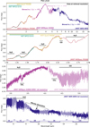 |
Fig. 1 Observations considered for the atmospheric characterization of PSO J318. Uppermost panel: all data considered for the spectral characterization of PSO J318at the wavelength binning fed into the retrieval and self-consistent grid model fits. Specifically, MIRI MRS data was binned down to λ/Δλ = 400, while NIRSpec G395H was binned to λ/Δλ = 400 and λ/Δλ = 1000 for NRS1 and NRS2, respectively. Second panel: HST WFC3, IRTF SpeX, and JWST NIRSpec PRISM data over the 1–3 μm wavelength range. Third panel: JWST NIRSpec G395H data at the full spectral resolution. Lowermost panel: JWST MIRI MRS data at the full spectral resolution. |
2.2 JWST data reduction
For the NIRSpec data reductions (both PRISM and G395H) we directly used the *x1d.fits files from the MAST data archive. We include the PRISM data from 1 μm onwards, and disregard it for wavelengths longer than 3 μm, since they exhibit a flux excess and unexpected systematic behavior when compared to the G395H data. Within our adopted range the NIRSpec data of PRISM and G395H are in good mutual agreement. PRISM also lines up with archival HST and IRTF observations at short, while G395H lines up with the bluest MIRI MRS channel (1A) at long wavelengths (see Fig. 1).
We performed our own reduction for the MIRI MRS data, using the public jwst pipeline1 (version 1.12.5, CRDS reference files jwst_1149.pmap, Bushouse et al. 2023). We started from the *uncal.fits files, and applied all three stages of the standard data reduction. Stage 1 produces *rate.fits files, that is, the rate of photoelectric charge accumulation on the detector. In Stage 2 the world coordinate system (wcs) is applied, and several calibrations are applied to produce photometrically calibrated *cal.fits files. The calibrations applied here include a flat field, stray light, residual fringe and photometric correction. Between Stage 2 and 3 we perform a nod subtraction between dither positions to reduce the residual background. Finally, Stage 3 projects the 2D spectra into 3D cubes (x/y/λ, *s3d.fits) using the “drizzle” weighting algorithm (Law et al. 2023). Here, we include an outlier detection, flagging remaining outliers due to, for example, cosmic rays. A one-dimensional spectrum (*x1d.fits) can then be extracted from this cube by placing an aperture of one Full Width Half Maximum (FWHM) of the corresponding Point Spread Function (PSF) around the source and measuring the contained flux at each wavelength. The mid-point of the source is detected using the ifu_autocen() built-in function.
We also applied an additional correction to the MRS data to account for large-scale systematics, which were apparent in the spectrum produced by the jwst pipeline. Examination of the IFU cubes revealed significant, wavelength-dependent structure in the background, even after the dither subtraction; this leads to wavelength-dependent systematics in the extracted spectrum when using the default pipeline. To correct for this systematic we follow the process described in Matthews et al. (2025). Briefly, we calculated the 3D cubes in the ifualign orientation, where the striping is largely horizontal. We then masked out the source and modeled the background structure for each individual λ slice in a data-driven fashion. This background can then be subtracted, and the spectrum extracted from the cube using the standard jwst pipeline methods. With this correction, our final spectra are smooth in the mid-infrared, well-explained with physical models, and show good agreement in the regions where consecutive sub-channels overlap.
2.3 Archival data
In addition to JWST observations we considered the archival NIR spectra taken with HST WFC3 by Biller et al. (2018). We included all spectra taken during five consecutive HST orbits in our analysis, spanning 7 hr, so almost one full rotation of the object. We also included ground-based archival NIR spectroscopy from IRTF SpeX, taken by Liu et al. (2013). This data set was included from wavelengths larger than 1 μm, out to wavelengths of 2.35 μm. Wavelengths shorter than 1 μm were excluded for numerical efficiency, and because PSO J318becomes increasingly faint (leading to low S/N data). Wavelengths longer than 2.3 μm were excluded because of low S/N. These archival data sets show good mutual agreement (neglecting the fact that HST is actually precise enough to show PSO J318’s variability), and agree well with JWST NIRSpec PRISM, see Fig. 1.
3 Characterizing PSO J318’s 10 μm silicate feature
The data we present in Fig. 1 exhibits a prominent absorption feature at ~10 μm, which we attribute to silicates, that is, absorption by condensed silicon-oxide-rich material in the atmosphere of PSO J318. Silicon is one of the most abundant refractory elements in the universe (e.g., Asplund et al. 2009). In its condensed form it constitutes a major opacity source, especially at 10 μm. In addition to the aforementioned brown dwarfs and planets, silicate absorption is evident in outflows of evolved AGB stars, ejecta of supernovae, proto-planetary and debris disks, the interstellar medium and AGN dust tori (for a detailed review see Henning 2010).
Since we posit that silicates cause the 10 μm absorption, in the following we explore what type of silicate material may be present in the atmosphere of PSO J318. For planets or brown dwarfs silicates of olivine-type stoichiometry (Mg2−xFexSiO4), pyroxene-type (Mg1−xFexSiO3) and quartz (SiO2) are expected species, with their relative importance likely determined by atomic abundance ratios such as Mg/Si (Calamari et al. 2024) and potentially C/O (Wetzel et al. 2013). The internal structure of silicates can be crystalline, that is, the elemental building blocks are arranged on a regularly repeating lattice, or amorphous. We note that the amorphous state is not well defined. It can range from configurations of small crystalline domains that do not properly connect to disarray on a smaller level, where crystalline ordering is missing altogether (Henning 2010). In studies of silicates forming around evolved stars and in proto-planetary disks it was found that crystalline silicates tend to be Fe-poor (e.g., Jaeger et al. 1998; Olofsson et al. 2009; Juhász et al. 2010), which is consistent with theoretical models predicting that Fe should be more abundant in amorphous silicates, that form at lower temperatures (Gail 2010).
Recent studies that investigated the broad silicate feature visible in Spitzer IRS spectra found that the 10 μm feature is best explained by amorphous silicate absorption. Luna & Morley (2021) constrained particle sizes to be small (≲0.1–1 μm), and consisting of SiO, MgSiO3, or Mg2SiO4. Suárez & Metchev (2023) found that the visible clouds consist of amorphous pyroxene-type (Mg1−x FexSiO3) material for low-gravity brown dwarfs (with particle sizes around 1 μm), while high-gravity brown dwarfs may be dominated by small (≲0.1 μm) grains composed of amorphous SiO and MgSiO3.
Since a 10 μm-feature of a putative silicate cloud appears to be present in PSO J318’s spectrum, we first attempt to study its grain properties based on the spectral shape from 7–13 μm alone in Section 3.1. This is done in an agnostic manner (i.e., neglecting the constraints on composition from Luna & Morley 2021; Suárez & Metchev 2023). This can be seen as a precursor step before turning to the numerically costly retrievals, which are presented in Section 3.2. We expect that the shape of the 10 μm feature is sensitive to the following particle properties:
Particle structure. Silicate crystals have sharp absorption features stemming from Si-O stretching transitions. In amorphous particles the crystal structure is lost. The corresponding distribution of bond lengths and angles in the resulting solid leads to a much wider, less structured absorption feature at 10 μm (Dorschner et al. 1995; Henning 2010). If condensation nuclei that form the seed particles for cloud particle growth are prevalent and mixing is slow, silicates in the atmospheres of exoplanets and brown dwarfs should condense at high temperatures, as soon as gas is mixed into regions where condensates are thermodynamically stable. This would result in crystalline particles, because amorphous grains are very efficiently and quickly converted into crystals at high temperatures (so-called annealing, see, e.g., Fabian et al. 2000; Gail 2001; Harker & Desch 2002; Gail 2004). The broad, presumably amorphous absorption features seen in VHS 1256b (Miles et al. 2023), PSO J318 and the Spitzer spectra of many brown dwarfs (Luna & Morley 2021; Suárez & Metchev 2023) are therefore unexpected and point to a gap in our understanding of cloud physics. We also note that, for some stoichiometries, multiple crystalline forms may exist, with distinct spectral features. The stability regimes of these so-called polymorphs depend on temperature. Conversion timescales between polymorphic phases at temperatures relevant for atmospheres are in the range of hours. This may also make the occurrence of mixed polymorph grains possible, which could further transition through an amorphous stage during polymorph transformation (Moran et al. 2024).
Particle composition. Particle composition has a large effect on the shape and the exact location of the 10 μm feature. For example, as one moves from quartz (SiO2) to enstatite (MgSiO3) to forsterite (Mg2SiO4) the degree of polymerization of SiO4 tetrahedra drops, leading to a shifting of the 10 μm feature to redder wavelengths (Henning 2010). The location and number of the narrow absorption maxima observed for crystalline silicates likewise changes as the composition of the grains is varied. Adding iron to the condensates described above (e.g., MgFeSiO4 instead of Mg2SiO4 when considering particles of olivine-type stoichiometry) further reddens the onset of the 10 μm band, because the bond lengths between Fe and O are longer than between Mg and O (Jaeger et al. 1998). This effect is clearly discernible in crystalline silicates. In amorphous silicates, however, it can be obscured by other factors, including differences in disorder, shape and size. In addition, it is not necessarily the case that cloud particles are composed of just one species. In principle, particles could be layered (one species condensing on top of another) or more strongly mixed. For mixed particles, the characteristic absorption features (e.g., crystalline absorption features) could be muted (Kiefer et al. 2024). The degree to which this is important is not clear, and we note that the silicate absorption seen in circumstellar disks can show both amorphous and crystalline features of uniquely identifiable species simultaneously (e.g., van Boekel et al. 2005; Juhász et al. 2010).
Particle shape. The most common assumption for the shape of a cloud particle is a sphere, which enables the use of Mie theory to calculate the cross-sections of particles (e.g., Bohren & Huffman 1983). This approximation is likely incorrect, especially for solid particles (e.g., consider the shape of a snowflake). Several treatment options exist, all of which are more numerically costly than a simple Mie treatment, and all of them require additional parameters to describe the deviation of a particle from a sphere. Examples are treating particles as distributions of hollow spheres (DHS, see Min et al. 2005), continuous distributions of ellipsoids (CDE, see Bohren & Huffman 1983) or to fully specify the shape of a grain and estimating its cross section using the discrete dipole approximation (DDA, see, e.g., Purcell & Pennypacker 1973; Draine 1988). The wavelength location of the crystalline absorption features can move significantly if deviations from spherical grains are considered, and indeed such a departure has been inferred for most of the crystalline silicate absorption in protoplanetary disks (e.g., Bouwman et al. 2001; Juhász et al. 2010). An example of how the particle shapes affect exoplanet transmission spectra with crystalline clouds can be found in Mollière et al. (2017). Amorphous silicate absorption is less strongly influenced by the assumed particle shape; it mainly changes the extent of the 10 μm-feature towards red wavelengths, while the blue onset of the feature is largely unaffected (e.g., Henning & Stognienko 1993; Min 2015).
Particle size (distribution). The particle size significantly affects the wavelength-dependent cross-sections of clouds. For example – as follows from Mie theory – scattering is strongest for wavelengths λ ≪ 2πr, where r is the particle radius, and decreases with λ−4 for wavelengths ≫ 2πr. In addition, the 10 μm silicate absorption feature begins to disappear for grains of sizes ≳1 μm, and its shape likewise depends on the particle size (e.g., Min 2015). It is therefore not surprising that also the particle size distribution plays an important role for determining the shape of the 10 μm absorption feature. Log-normal particle size distributions, which appear symmetric around a characteristic size in logged particle size are a common assumption (e.g., Ackerman & Marley 2001; Morley et al. 2012; Nasedkin et al. 2024; Morley et al. 2024, to name just a few studies). Another example is the Hansen distribution (Hansen 1971; Burningham et al. 2021; Vos et al. 2023) which can be asymmetric, depending on the choice of parameters, and may exhibit broad shoulders. Finally, there are fully microphysical models that solve for the particle size distribution as a function of altitude by considering processes such as condensation, settling, and coagulation, etc. (e.g., Helling et al. 2008; Gao et al. 2018; Powell et al. 2018). These studies often point to complex, multi-modal distributions, although it should be explored which particle sizes inferred from this full treatment actually matter when calculating spectra. In addition, it is not likely that cloud properties are constant across the atmosphere of a planet or brown dwarf, which can affect the aggregate shape of the 10 μm feature that arises from averaging fluxes across the visible hemisphere of the object.
Even if the above properties of the cloud species were perfectly known, biases are likely to impact analyses due to the challenges of deriving optical constants in laboratories. For instance, samples of the species of interest may be hard to synthesize. One way of producing amorphous silicates is through melts in a high-temperature furnace and subsequent cooling (with rates of ~1000 K/s) to prevent crystallization (Jäger et al. 1994; Dorschner et al. 1995). Such samples are called “glassy” in the following. However, while MgFeSiO4 has a melting point of manageable 1900 K, Mg2SiO4 only melts at ~2200 K, which is hard to achieve in a laboratory setting. For such species the so-called sol-gel method is used, where metal organic compounds are dissolved in mixtures of water and alcohol (methanol or ethanol), hydrolized and finally condensed as a three-dimensional magnesium silicate network, the “silicate gel” (see, e.g., Jäger et al. 2003a). The condensed gel is then distilled in order to remove the water and alcohol present, and subsequently annealed at elevated temperatures in order to remove the porosity and to densify the material (but not enough to let it crystallize). A challenge associated with silicate samples produced by melting or by the sol-gel method is the derivation of optical constants at wavelengths corresponding to low absorption. The best solution would be transmission measurements of thick samples to determine the absorption coefficient directly from the transmission. If this is not possible, extrapolation is a commonly employed solution. However, this can result in discrepancies in the optical data close to the blue onset of the 10 μm feature between the silicates generated by melting or by sol-gel.
A last complication we want to mention here is that optical properties of a material sample depend on its temperature. This is most important for the absorption features of crystalline silicates where peaks become broader and shift location for higher temperatures (e.g., Zeidler et al. 2015). Interestingly, this may affect the 10 μm feature somewhat less compared to the longer wavelength silicate absorption features towards the far-infrared (λ ≳ 30 μm, see Koike et al. 2006). In all analyses in this work we neglect the temperature dependence of the silicate opacities. This is a common, but not necessarily justified, assumption in the community.
3.1 Silicate feature analysis with the brightness temperature method
Given the aforementioned complexities that influence what the 10 μm absorption of a cloud will look like, it would be preferable to have an efficient method for identifying cloud candidate species in a first-look approach, that is, before running numerically costly retrievals. We present and apply a potentially useful method for this in the following. Since we treat this demonstration as a proof of principle, only a subset of the cloud complexities was explored in this study.
3.1.1 Fitting procedure
In an optically thin slab of gas and condensates, information about the silicates could be extracted by directly comparing the observed flux F(ν), where ν is the spectral frequency, to predicted opacities κ(ν), where opacity is defined as cross-section per unit mass. This is because in the optically thin limit the flux is described by
![Mathematical equation: $\[F(\nu) \propto \kappa(\nu) B(\nu, T),\]$](/articles/aa/full_html/2025/11/aa55732-25/aa55732-25-eq5.png) (1)
(1)
where B(ν, T) is the Planck function, and T is the silicate dust temperature. The atmosphere of a giant planet or brown dwarf is never optically thin. Instead, at every frequency one can only probe into the atmosphere until it becomes optically thick, which defines the so-called photosphere. Commonly the optical depth at the photosphere is assumed to be τ ≈ 2/3, although we note that emission is a continuous process, and the observed flux arises from regions at both lower and higher τ. The above relation then no longer holds but can be replaced by an expression that relates the atmospheric brightness temperature, Tbright, to the opacity if making the simplifying assumption that the flux is emitted from τ = 2/3 exactly (or another fixed point):
![Mathematical equation: $\[\ln [\kappa(\nu)] \approx-\frac{\ln \left[T_{\text {bright}}(\nu)\right]}{\nabla}+\operatorname{cst},\]$](/articles/aa/full_html/2025/11/aa55732-25/aa55732-25-eq6.png) (2)
(2)
where ∇ = dln(T)/dln(P) is a power law index approximating the average temperature gradient of the atmosphere in the regions probed by the observations and cst is a place holder for a constant that is irrelevant to the problem. The derivation of this expression, a list of assumptions that go into obtaining it, and a discussion of the validity of these assumptions are presented in Appendix A. As long as the cloud is the dominant opacity source over the frequency range of interest, an approximated cloud opacity can be extracted, up to a scaling constant, from the measured brightness temperature.
In what follows, we use Eq. (2) to fit the opacities predicted for various silicate species to the observed brightness temperature. In practice, we assume that the silicate cloud resides in a cloudy column of the atmosphere, and add a correction to the brightness temperature to account for the emission of another atmospheric column with a constant brightness temperature. In the derivation this column is called “clear”, but its defining property is that its spectrum is featureless (i.e., at constant brightness temperature) across the 10 μm region. We treat ∇, the cloud column coverage f and the clear column photospheric temperature (again, see Appendix A for more details) as free parameters to extract ln(κ). This ln(κ) is then compared to predicted silicate cloud (scattering+absorption) opacities, assuming a log-normal particle size distribution (in principle, any distribution may be adopted). For this, the mean particle size and width of the distribution are free parameters. The maximum of the log-opacity of the resulting cloud description is scaled to the maximum of the log-opacity derived from the brightness temperature, with an additional scaling (additive term in log space) as a free parameter. We note that all free parameters are varied simultaneously during the fit. We then investigate which species best describes the 10 μm feature over a wavelength range from 8–12.5 μm, which we determined to be the range over which the silicate cloud is the dominant opacity contributor. The priors adopted for the free parameters are given in Table 1. The fits were run by estimating the posterior probability distribution of the free parameters, given the observed brightness temperatures. For this we used PyMultiNest (Buchner et al. 2014), which is a Python wrapper of MultiNest (Feroz & Hobson 2008; Feroz et al. 2009, 2019). For our runs we assumed 200 live points, and the standard parameter values of pymultinest.run(), that is evidence_tolerance = 0.5 and sampling_efficiency = 0.8. The error bars on the brightness temperature observations were derived from the flux uncertainties (see Section A.3). For the latter we used the error bar inflation from our best-fitting retrieval model (b = −8.589 at λ/Δλ = 400, see Section 3.2 for more information), adjusted to our fitting resolution λ/Δλ = 100.
The ![Mathematical equation: $\[\chi_{\text {red }}^{2}\]$](/articles/aa/full_html/2025/11/aa55732-25/aa55732-25-eq7.png) values for all considered silicate species are given in Table 2 (see Table B.1 for a list of references of the optical constants). The fits of the “top 14” species can be seen in Fig. 2 and fits of all remaining species are shown in Figure D.1. We find that the best-fit
values for all considered silicate species are given in Table 2 (see Table B.1 for a list of references of the optical constants). The fits of the “top 14” species can be seen in Fig. 2 and fits of all remaining species are shown in Figure D.1. We find that the best-fit ![Mathematical equation: $\[\chi_{\text {red }}^{2}\]$](/articles/aa/full_html/2025/11/aa55732-25/aa55732-25-eq8.png) are smaller than one, which could indicate overfitting. We note, however, that the flux error bars we are using here have been scaled up, based on values found in the full retrievals (see Sect. 3.2), and may account for both underestimated uncertainties and retrieval model insufficiencies.
are smaller than one, which could indicate overfitting. We note, however, that the flux error bars we are using here have been scaled up, based on values found in the full retrievals (see Sect. 3.2), and may account for both underestimated uncertainties and retrieval model insufficiencies.
In addition to the nominal single-species fits described here, we also attempted to fit the silicate feature by combining two cloud species. For this we considered all Nc(Nc − 1)/2 = 276 possible combinations of species, where Nc = 24 is the number of Si-bearing cloud species in our database. To keep the number of free parameters low, we only added a relative weighting between the two species as an additional free parameter (κtot = κ1 + wκ2, with w going from 10−5 to 105 on a log-uniform prior). The mean particle size and width of the size distribution was therefore the same for both species. We robustly find that SiO is the species leading to the best fits: it is one of the two combined species in 21 out of the top 25 combinations, and also is present in the best combination. We find that adding an additional species can increase the fit quality, pushing ![Mathematical equation: $\[\chi_{\text {red }}^{2}\]$](/articles/aa/full_html/2025/11/aa55732-25/aa55732-25-eq9.png) to values as low as 0.52, when compared to the single-species best-fit (also SiO) of 0.65. We refrained from a more detailed exploration with multiple species, because we considered the brightness temperature technique as a tool for finding likely cloud candidates for in-depth analyses via retrievals here. The underlying assumptions (see Appendix A) may be satisfactorily met for our intended purposes, but may not be good enough to replace an in-depth retrieval analysis over the full wavelength range, with proper radiative transfer. For crystalline silicate features, for which cloud species have more distinct appearances for different species, the multi-species approach may be worth revisiting.
to values as low as 0.52, when compared to the single-species best-fit (also SiO) of 0.65. We refrained from a more detailed exploration with multiple species, because we considered the brightness temperature technique as a tool for finding likely cloud candidates for in-depth analyses via retrievals here. The underlying assumptions (see Appendix A) may be satisfactorily met for our intended purposes, but may not be good enough to replace an in-depth retrieval analysis over the full wavelength range, with proper radiative transfer. For crystalline silicate features, for which cloud species have more distinct appearances for different species, the multi-species approach may be worth revisiting.
Priors adopted for the cloud feature fit.
Ranked list of cloud opacity fits using the brightness temperature method for the wavelength range of 8–12.5 μm.
3.1.2 Results of the brightness temperature analysis
The most likely cloud species, if taking the results of the brightness temperature method at face value, is the absorption of amorphous SiO. This is surprising, because SiO would oxidize to form SiO2 very quickly. If correct, this could mean that the SiO forms in a quite strongly O-depleted (relative to carbon) environment (Wetzel et al. 2013), or that we trace the formation of SiO nuclei that form the seeds for further cloud condensation (e.g., Gail et al. 2013) (this option is discussed further in Sect. 4.3.2, since we deem it a possible scenario). One may argue that while SiO fits the spectrum well over the narrow wavelength range considered here (8–12.5 μm), the required particle properties may lead to imperfect fits over the full JWST wavelength range. We thus progressed by using the brightness temperature method as a way to inform our decision on which condensate species should be tested in retrievals. However, as we describe in Section 3.2, the retrievals also point to SiO being the most likely species. We also note again that SiO was identified as a possible species in (Luna & Morley 2021; Suárez & Metchev 2023). The implications of this finding, if correct, are discussed in Sections 4.3.2 and 5. Lastly we note that even for the best-fitting species a residual wavelength-dependent structure is visible in the opacities inferred from brightness temperatures, from ~9.5–10 μm, see Fig. 2. Likewise, we discuss this in Section 4.3.2.
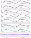 |
Fig. 2 Opacity fits of the 10 μm feature for the “top 14” silicate cloud species using the brightness temperature method. The remaining fits for the less well fitting species can be found in Fig. D.1. |
3.2 Retrievals
Armed with a ranked list of likely cloud species, we study how well we can reconstruct the spectrum of PSO J318through retrievals below, and how robustly we can constrain the underlying properties of the atmosphere. Particular focus is placed on the identity of the clouds causing the 10 μm feature. More specifically, we tested the top eight species identified with the brightness temperature method. In addition, we looked at three more species from further down in the list, resulting in 11 species with ![Mathematical equation: $\[\chi_{\text {red }}^{2}\]$](/articles/aa/full_html/2025/11/aa55732-25/aa55732-25-eq59.png) values from 0.65 to 4 in the brightness temperature method (these species are also marked with an asterisk in Table 2).
values from 0.65 to 4 in the brightness temperature method (these species are also marked with an asterisk in Table 2).
Retrievals generally aim to constrain the probability distribution of parameters thought to describe the atmosphere (e.g., temperature, composition, cloud properties) while leveraging any prior beliefs we have about the distribution of said parameters. A fairly recent review on retrievals can be found in Madhusudhan (2018). A number of retrieval codes exist now, many of them open source; we refer the reader to MacDonald & Batalha (2023)2 for an up-to-date list. In the work presented below we use petitRADTRANS (pRT, see Mollière et al. 2019, 2020; Blain et al. 2024); retrievals were run with pRT’s retrieval package described in Nasedkin et al. (2024).
3.2.1 Forward model description
The forward model is the function that returns flux predictions given a set of atmospheric input parameter values. A retrieval inverts the forward model and returns the parameter distribution, given an observation. The forward model is thus the central ingredient of any retrieval. We start by defining a single-column forward model which takes the atmospheric temperature, cloud and compositional structure as input parameters for calculating the flux emerging at the top of the atmosphere (including multiple scattering). A single-column model can also be used as a building block to approximate horizontal atmospheric heterogeneities. For this we assume that the atmosphere is well described by the flux predicted from a set of one-dimensional columns, weighted by the fractional area they occupy in the atmosphere. Below we assume at most two columns.
Atmospheric temperature structure. We described the atmospheric temperature structure using the approach reported in Zhang et al. (2023), that is, the power law dependence of the temperature with pressure dlnT/dlnP was retrieved at 10 points in the atmosphere (equidistantly spaced in log-pressure), and quadratically interpolated between these layers. The priors for the seven lowest (i.e., highest pressure) points were determined from constructing the distribution of dlnT/dlnP for the temperature profiles reported in Morley et al. (2024), as has been reported in Zhang et al. (2025). The corresponding 1-σ ranges of these distributions defined our Gaussian priors. In the three uppermost layers the power law index could vary freely (excluding inversions) because our pressure range extends to 10−6 bar, but the Morley et al. (2024) models end at 10−4 bar. The adopted priors for all retrieval parameters and the pressure coordinates of the 10 points are given in Table 3.
Temperature excursion. We additionally allow for the temperature profile to deviate from the above treatment. This is only used for some multi-column setups. Nominally, the columns share the same temperature profile, but when applying the excursion treatment the temperature structure of a given column is allowed to deviate. The temperature excursion is defined by multiplying the nominal dlnT/dlnP structure by
![Mathematical equation: $\[1+f_{\mathrm{exc}}\left(1-\frac{2|\log _{10}(P)-\log _{10}(P_{\mathrm{exc}})|}{\Delta \log _{10}(P_{\mathrm{exc}})}\right),\]$](/articles/aa/full_html/2025/11/aa55732-25/aa55732-25-eq60.png) (3)
(3)
for all |log10(P/Pexc)| ≤ Δlog10(Pexc)/2. The prior for fexc is chosen such that the resulting behavior of the excursion spans from P-T curves exhibiting (weak) inversions to curves with strong boosts of the dlnT/dlnP gradient. Also, log10(Pexc) and Δlog10(Pexc) are free parameters.
Chemical composition. We determined the chemical composition by prescribing chemical equilibrium for all absorber species we expect to play a minor role. For this we retrieved the atmospheric metallicity, [M/H], and C/O, where the latter was changed by scaling the oxygen abundance after all metals have been scaled by 10[M/H]. The composition is obtained by interpolating in the chemical equilibrium table that is part of pRT, which itself has been prepared with easyCHEM (Lei & Mollière 2024)3. No rainout is included in these calculations, while it is implicitly taken into account for some species by limiting the selection of condensates. For example, feldspars such as orthoclase are not included in our chemical calculations, with the goal of preventing a sequestration of alkalis into these species at the temperatures of L/T transition objects – which is not observed (Line et al. 2017; Zalesky et al. 2019). Since we wanted to treat the major absorbing species more flexibly, we retrieved the mass fractions of 12CO, 13CO, CO2, CH4, CrH and H2O independently, assuming them to be vertically constant. CrH was retrieved independently because it is not included in the precomputed equilibrium table of pRT. The retrieved metallicity and C/O values reported in Table 6 are obtained from considering all metal gas phase abundances, irrespective of whether they were obtained from the chemical interpolation or retrieved independently.
Gas opacity sources. We included the following line opacities in our analysis: CH4 (Hargreaves et al. 2020), 12CO (Rothman et al. 2010), 13CO (Rothman et al. 2010), CO2 (Yurchenko et al. 2020), CrH (Burrows et al. 2002), FeH (Wende et al. 2010), HCN (Barber et al. 2013), H2O (Polyansky et al. 2018), H2S (Azzam et al. 2016), K (line profiles by N. Allard, see Mollière et al. 2019), Na (Allard et al. 2019), NH3 (Coles et al. 2019), PH3 (Sousa-Silva et al. 2014), SiO (Yurchenko et al. 2021), TiO (McKemmish et al. 2019). Where available, correlated-k opacities in the pRT format were taken from the ExoMolOP database (Chubb et al. 2021) or computed with the method described in Mollière et al. (2015) otherwise. Rebinning to lower resolution opacities was done using Exo_k (Leconte 2021).
Clouds. The parameterized behavior of the clouds is motivated by the semi-analytical model presented in Ackerman & Marley (2001), but is more flexible. For any given cloud species we freely retrieve the position of the cloud base, Pi,base. The cloud mass fraction at the cloud base Xi,base, where i stands for a cloud species like MgSiO3, is found by scaling the elemental mass budget by a free parameter 10si. The elemental mass budget is determined by locking all elemental building blocks into the condensate in question, until the first species is depleted (e.g., for MgSiO3 the limiting element is Si, when considering scaled solar composition). The cloud mass fraction in the atmosphere is then Xi(P) = Xi,base(P/Pi,base)fsed,i for P ≤ Pi,base and 0 for P > Pi,base. The power law index fsed is likewise a free parameter. The particle size distribution is assumed to be log-normal, as defined in Ackerman & Marley (2001), with the mean particle size a and the width σ as free parameters in our standard approach. We set the prior for σ up in the same way as in the brightness temperature fitting, see Section 3.1.
Evolutionary priors. Despite excellent data, we noticed the tendency of our retrievals to approach unphysical values for bulk parameters (e.g., log(g) → 3 and lower, depending on the prior range). We therefore decided to prescribe priors on the radius and log(g), using the values derived in Zhang et al. (2020). For these values the authors assumed an age for PSO J318 consistent with the β Pic moving group (24 ± 3 Myr), used PSO J318’s inferred bolometric luminosity, and the cooling curves by Saumon & Marley (2008). Alternatively we adopted free priors on the radius and gravity to explore their effect on our best-fitting model.
Column coverage. Our forward model is set up in such a way that it can handle multiple 1D columns, with the total flux being
![Mathematical equation: $\[F=\sum_{i=1}^{N_{\text {column }}} b_i F_i,\]$](/articles/aa/full_html/2025/11/aa55732-25/aa55732-25-eq64.png) (4)
(4)
where Fi is the top-of-atmosphere flux of column i, and bi ≥ 0 is its weight, respectively. In principle, the different columns may be fully independent, but in practice they share most of their parameters and only the cloud parameters are varied on a percolumn basis, for example. Because the retrievals presented here assumed at most two columns we defined b1 = B, b2 = 1 − B, B ≤ 1. Since the various data sets we considered were taken at different epochs, we retrieved three different values, BHST, BSpeX, and BJWST, which are thought to express different average climate states at the respective times of observation with the three observatories. That is, if ![Mathematical equation: $\[\tilde{B}(t)\]$](/articles/aa/full_html/2025/11/aa55732-25/aa55732-25-eq65.png) is the actual time-dependent change due to rotation of the object, then B is the time average of
is the actual time-dependent change due to rotation of the object, then B is the time average of ![Mathematical equation: $\[\tilde{B}(t)\]$](/articles/aa/full_html/2025/11/aa55732-25/aa55732-25-eq66.png) during the observation. We neglect that the JWST observations with the NIRSpec PRISM, G395H, and MIRI MRS instruments were taken sequentially and thus recorded time-averaged fluxes from different rotational phase intervals.
during the observation. We neglect that the JWST observations with the NIRSpec PRISM, G395H, and MIRI MRS instruments were taken sequentially and thus recorded time-averaged fluxes from different rotational phase intervals.
Uncertainty scaling. the flux uncertainties of individual instruments were scaled by setting σscaled.(λ) = [σ2(λ) + 10b]1/2, where σ is the reported flux uncertainty of the observation. This treatment allows for the correction of underestimated uncertainties or shortcomings in the model that would lead to systematic biases. It serves to give a more conservative estimate of the parameter distribution width, as it widens the posteriors (Line et al. 2015). The b values were retrieved on a per-data-set basis, where G395H’s NRS 1 and NRS 2 detectors were treated separately, because we binned NRS 1 to λ/Δλ = 400 and NRS 2 to λ/Δλ = 1000 during the retrievals. The priors for the b values were taken from Line et al. (2015).
Retrieval priors adopted for the single-column forward model.
3.2.2 Retrieval runs
We tested a number of different forward model setups in which the atmosphere was approximated by two columns. For example, we let the temperature structure vary between the columns, or the free parameters associated with the cloud, or the parameters associated with the chemical composition, or mixtures of these setups. The motivation for these options are the various processes (cloud cover, temperature, compositional variations) that have been suggested as drivers for atmospheric variability (see, e.g., Radigan et al. 2014; Robinson & Marley 2014; Tremblin et al. 2020). For studying whether we can constrain the most likely cloud species with retrievals we finally adopted a model in which both columns shared most of their properties: P-T structure, gas phase abundances, and the parameters describing the iron cloud. A global iron cloud (in the lower atmosphere) is a common finding in retrieval studies (Burningham et al. 2021; Vos et al. 2023). Then, for Column 1, a silicate cloud with its associated parameters was retrieved, while for Column 2 the silicate cloud was neglected (by setting ssilicate = −50), motivated by the patchy silicate cloud findings of, for example, Apai et al. (2013); Vos et al. (2023); Zhang et al. (2025). We thus stress that “patchy silicate clouds” does not mean that the atmosphere is described by a cloudy and a cloud-free column, since the iron cloud is present in both columns. The two Columns 1 and 2 also retrieved separate Δlogσ, allowing for different widths of the particle size distributions between Columns 1 and 2. Results obtained with retrieval models that differ from our standard setup, for example assuming a single-column atmosphere, or keeping the cloud parameters fixed in both columns and varying the temperature structure instead, or turning off the evolutionary prior, are listed in Table 6 and discussed in Section 4.3.
We note that among all our explored two-column setups, the fiducial model definition described above consistently fit the data with the least bias upon visual inspection, resulted in the smallest required error bar scalings (i.e., the smallest b-factors), and formally converged in retrievals most reliably. The best-practice approach would be to carry out model selection via a Bayes factor analysis, but with our 40+ free parameters, wide wavelength coverage, and high S/N-data, MultiNest starts to break down (also see Buchner 2023; Himes 2022; Dittmann 2024, for a discussion of how nested sampling can fail). For example, we found that models with too many free parameters failed to converge, or observed that widening the prior ranges (when turning off the evolutionary priors for log10(g) and R) resulted in worse fits for a given model. Given the fact that we are in a high-dimensional parameter space (with signs of the sampler missing the global likelihood maximum, also see Himes 2022), and given that we must run MultiNest in constant sampling efficiency to enable convergence (which can lead to over-confident posteriors, see Chubb & Min 2022), we refrain from carrying out MultiNest-based Bayes factor analyses; we cannot guarantee that the posterior sampling leads to a reliable integration for the evidence Z. This observation and its implications for the use of nested sampling in the era of JWST (and ELT in the future) are discussed in Section 5.
In practice, we set up MultiNest with 3000 live points, using const_efficiency_mode=True, sampling_efficiency = 0.05 and evidence_tolerance set to 0.5. While MultiNest results must be approached cautiously for the reasons stated above, it is the nested sampling algorithm that converges most efficiently (Himes 2022) and enables us to run retrievals for this study in the first place. To speed up the retrievals further we binned the MIRI MRS data to pRT’s wavelengths for a λ/Δλ = 400 wavelength spacing, exactly. The same was done for NIRSpec G395H NRS1. For NRS2 we used the spacing of pRT wavelength tables at λ/Δλ = 1000, to retain sensitivity to secondary CO isotopologues. For HST, SpeX and JWST NIRSpec PRISM the models were calculated at λ/Δλ = 300 (HST) and 140 (SpeX and NIRSpec PRISM) before being convolved to R = 130 (HST), 75 (SpeX) and 65 (NIRSpec PRISM) and then binned to the data’s respective wavelength spacing. Retrievals were run on the Viper cluster of the Max Planck Computing & Data Facility (MPCDF), each requiring on the order of 105 core hours to finish on AMD EPYC Genoa 9554 CPUs; each retrieval ran for about a week on 1000 cores.
3.2.3 Retrieval results
Figure 3 shows the best-fitting spectra of the two-column retrieval models. Panel a shows our “winning model”, that is, the model with the lowest Bayesion information criterion (BIC; see discussion below); an atmosphere with a global iron cloud; and a patchy SiO cloud with amorphous spherical particles, plotted on top of the JWST observations. Residuals (Panel b) are mostly flat but exhibit systematic behavior at some locations, for example in the water band at 6.6 μm. In panels c–m, we show retrievals with all tested cloud candidate species, zoomed in on the silicate feature. In these zoomed-in views it can be seen that the predicted line depth appears to be shallower than the data from 7–8 μm for some of the models. In general, the winning model retrieval finds that the flux of PSO J318is significantly reddened by clouds, since neglecting the cloud opacity for the best-fit model leads to a dramatic increase of flux in the NIR. What is more, the flux separates into a column component that is very red and blackbody-like, and one that retains molecular features much more strongly, similar to the results presented for 2M1207b in Zhang et al. (2025).
Evidence values from nested sampling cannot be used in the selection of the most likely model from our set of tested models, but we still wanted to tentatively vet the retrievals with different cloud species for fit quality (assuming that the global log-likelihood maximum, or a maximum of similar quality to the global maximum, was identified). For this, we made use of the BIC, BIC = Nparamln(Nλ) − 2ln(Lmax), which allows for model selection. Here, Nparam is the number of free parameters of the model, Nλ is the number of wavelength points in the spectrum, and ![Mathematical equation: $\[\text{ln} L_{\text {max}}=-0.5 {\sum}_{i=1}^{N_{\lambda}}\{(f_{i}-m_{i}^{\text {best}})^{2} /(\sigma_{i}^{2}+10^{b})+\ln [2 \pi(\sigma_{i}^{2}+ 10^{b})]\}\]$](/articles/aa/full_html/2025/11/aa55732-25/aa55732-25-eq67.png) is the best-fit log-likelihood, where
is the best-fit log-likelihood, where ![Mathematical equation: $\[f_{i}, m_{i}^{\text {best}}\]$](/articles/aa/full_html/2025/11/aa55732-25/aa55732-25-eq68.png) and σi are the observed flux, best-fit model, and observational uncertainties at Nλ wavelengths λi, respectively, and b is the error bar scaling parameter. The BIC makes the underlying assumption that posteriors are multivariate Gaussians. This is not necessarily the case, but tends to be better satisfied in high S/N regimes, over which the retrieval model can be better linearized over the width of the posteriors. Yet, this is a limitation that needs to be kept in mind, especially if a posterior exhibits parameter correlations over wide value ranges, or is multi-modal. We note that from visual inspection, most of our retrieved parameters are tightly constrained, with mono-modal posteriors. If the a-priori probability for a given model is unknown (i.e., all models are considered to be equally likely before being applied to the data), then the probability ratio of two models ℳ1 and ℳ2, given the data vector f, P(ℳ1∣f)/P(ℳ2∣f), is given by the Bayes factor B12 = Z1/Z2. Z is the evidence here, which is typically returned by nested sampling. For a posterior with a shape described by a multivariate Gaussian one can write Z = exp(−BIC/2) (Raftery 1995). Since the models that test different silicate cloud species have the same number of free parameters and wavelength points, it then holds that
and σi are the observed flux, best-fit model, and observational uncertainties at Nλ wavelengths λi, respectively, and b is the error bar scaling parameter. The BIC makes the underlying assumption that posteriors are multivariate Gaussians. This is not necessarily the case, but tends to be better satisfied in high S/N regimes, over which the retrieval model can be better linearized over the width of the posteriors. Yet, this is a limitation that needs to be kept in mind, especially if a posterior exhibits parameter correlations over wide value ranges, or is multi-modal. We note that from visual inspection, most of our retrieved parameters are tightly constrained, with mono-modal posteriors. If the a-priori probability for a given model is unknown (i.e., all models are considered to be equally likely before being applied to the data), then the probability ratio of two models ℳ1 and ℳ2, given the data vector f, P(ℳ1∣f)/P(ℳ2∣f), is given by the Bayes factor B12 = Z1/Z2. Z is the evidence here, which is typically returned by nested sampling. For a posterior with a shape described by a multivariate Gaussian one can write Z = exp(−BIC/2) (Raftery 1995). Since the models that test different silicate cloud species have the same number of free parameters and wavelength points, it then holds that
![Mathematical equation: $\[\text{ln} B_{12} \approx \frac{1}{2}\left(\chi_2^2-\chi_1^2\right)+\frac{1}{2} \sum_{i=1}^{N_\lambda} \ln \frac{\sigma_i^2+10^{b_2}}{\sigma_i^2+10^{b_1}},\]$](/articles/aa/full_html/2025/11/aa55732-25/aa55732-25-eq69.png) (5)
(5)
where ![Mathematical equation: $\[\chi^{2}={\sum}_{i=1}^{N_{\lambda}}(f_{i}-m_{i}^{\text {best }})^{2} /(\sigma_{i}^{2}+10^{b})\]$](/articles/aa/full_html/2025/11/aa55732-25/aa55732-25-eq70.png) . We note that our error bar scaling via 10b causes a χ2 → Nλ convergence in retrievals (Line et al. 2015), unless b priors are hit, which we observe for the worst cloud candidates. However, the above expression takes this into account: in a situation where all χ would indeed be identical, the model with the least upscaled error bars would win. Given a Bayes factor between a given model and the one with the highest evidence, it is customary to calculate a rejection significance using the formalism described in Benneke & Seager (2013). However, Kipping & Benneke (2025) recently argued that this is misleading, since the so-derived significance values are upper limits only. We thus refrain from a significance conversion and simply report Bayes factors.
. We note that our error bar scaling via 10b causes a χ2 → Nλ convergence in retrievals (Line et al. 2015), unless b priors are hit, which we observe for the worst cloud candidates. However, the above expression takes this into account: in a situation where all χ would indeed be identical, the model with the least upscaled error bars would win. Given a Bayes factor between a given model and the one with the highest evidence, it is customary to calculate a rejection significance using the formalism described in Benneke & Seager (2013). However, Kipping & Benneke (2025) recently argued that this is misleading, since the so-derived significance values are upper limits only. We thus refrain from a significance conversion and simply report Bayes factors.
Panels c-m of Fig. 3 shows the best-fit models of all tested silicate species on top of the data, zoomed in on the 10 μm region. In agreement with the brightness temperature method, the winning silicate species of the two-column retrievals is amorphous SiO in the form of spherical particles. The panels also list the rejection Bayes factor of the respective cloud species, when compared to the winning SiO model. This Bayes factor was calculated using the best-fit log-likelihood from the full wavelength range (1–18 μm). After irregularly shaped amorphous SiO, the next most likely cloud consists of irregularly shaped glassy (thus amorphous) MgSiO3 particles, followed by crystalline spherical MgSiO3 particles. We note that crystalline MgSiO3 appears unlikely, given the smoothness of the 10 μm feature visible in the data. Indeed, any amorphous material with pyroxene-type (Mg1−xSixO3) stoichiometry appears to be fitting the data better across the 10 μm region plotted in panels c–m, but we note again that the rejection Bayes factors are calculated over the full wavelength range. The best fit spectra of all tested retrieval models, over the full wavelength range from 1–18 μm, are shown in Fig. C.1.
We list the ΔBIC and corresponding rejection Bayes factors of less favored cloud species in Table 4. In comparison, the Bayes factors returned by MultiNest did not lead to believable results. For example, the BIC-based values indicate that spherical SiO is clearly favored over irregularly shaped SiO (log10(B) = 12.28). In contrast, the corresponding Bayes factor from MultiNest results in a numerical overflow.
It is worth noting that the second most likely species identified by the retrievals is glassy amorphous MgSiO3. MgSiO3 is potentially expected to form in a PSO J318-like atmosphere, while the presence of SiO is surprising (Calamari et al. 2024, but also note Luna & Morley 2021; Suárez & Metchev 2023). As can be seen in panels e and g in Fig. 3, glassy MgSiO3 in spherical or irregular form actually leads to a good fit across the 10 μm range, albeit worse than the still favored SiO. In addition, both glassy MgSiO3 clouds lead to a too strong flux decrease in the predicted 4 μm flux peak of PSO J318 (see Fig. C.1), such that in total glassy MgSiO3 is disfavored with log10(B) = 32.18 and log10(B) = 42.81 respectively, when compared to SiO (see Table 4).
Comparing the ranked lists of likely cloud species in Tables 2 and 4, we conclude that the brightness temperature method can be a useful pointer for the most likely silicate absorbers affecting a spectrum. More specifically, the best and worst species in both lists agree, while there is some reordering present for the species in between (we note that only 11 of the 24 silicate species were tested in full retrievals due to the significant numerical cost). The brightness temperature method therefore must not be trusted blindly, but appears to lead to reasonably accurate predictions for PSO J318.
It is interesting that both the brightness temperature method and the retrievals come to the conclusion that the winning species is SiO. Making this assertion based on the shape of the amorphous 10 μm feature may still appear to be risky. But we note that the high altitude of the silicate cloud deck and the small particle sizes we retrieved, similar to the results presented in Luna & Morley (2021), also point to SiO, which we discuss in Section 4.3.2. The implication of this likely SiO detection is also further discussed in Section 5.
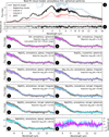 |
Fig. 3 Model fits of PSO J318 obtained with our fiducial two-column retrieval setup, considering different types of silicate clouds. Panel a shows the best-fit spectrum of the overall winning model (black solid line) plotted on top of the JWST data (gray circles, with 10b error scaling). The winning model assumes amorphous spherical SiO particles. The flux contribution of the two individual columns is also shown, at their best-fit relative scaling (salmon and rose colored lines, respectively). The light blue line shows the result of recalculating the best-fit model, but turning off the cloud opacities. Panel b shows the residuals between the best-fit model and the data (with 10b error scaling). Panel c is a version of Panel a that zooms in on the silicate feature, but the best-fit model is shown in pink instead. Panels d–m show the same zoomed-in view of the silicate feature but for the other tested silicate feature candidates. Panel n shows the residuals between model and data for the various silicate cloud species using the same colors as in panels c–m. |
Ranked list of likely cloud species obtained from full retrievals.
4 Bulk and atmospheric properties of PSO J318
In addition to constraining the identity of PSO J318’s silicate cloud species, its spectrum should also allow us to constrain bulk and atmospheric properties of the object. An established way to judge the accuracy of such constraints is to compare results obtained with retrievals to those obtained from interpolating in so-called self-consistent model grids. Such models determine the atmospheric structure by assuming radiative-convective equilibrium, coupled to chemical schemes that determine the atmospheric composition for a given atmospheric temperature structure and elemental abundances (e.g., Marley & Robinson 2015; Hubeny 2017). For the comparison below, we derived posterior distributions of the self-consistent model parameters with PyMultiNest, using interpolated model grid spectra as the forward model. This analysis was carried out with species4 (Stolker et al. 2020).
4.1 Radiative-convective equilibrium models
Self-consistent models have far fewer free parameters than retrievals, because they implement atmospheric physics to determine the atmospheric state to a much greater degree. A common free parameter is the composition. It is usually expressed through atmospheric metallicity [M/H] and through C/O. Other free parameters are the atmospheric gravity log10(g), the planetary effective temperature Teff, and parameters that describe the setup of the atmospheric clouds and departures from chemical equilibrium. In the following we describe the parameter grids we consider for our study. These are identical to the grids recently used in the Early Release Science (ERS) team’s paper on VHS 1256b, an object similar to PSO J318 (Petrus et al. 2024). A table of the free parameters, the explored parameter range, grid spacing and fit results is given in Table 5.
Exo-REM (Baudino et al. 2015; Charnay et al. 2018; Blain et al. 2021) solves for the atmospheric structure in radiative-convective equilibrium and implements chemical disequilibrium using the quench approximation (Zahnle & Marley 2014). Clouds are described following a combination of the time scale approach of Rossow (1978) with the Ackerman & Marley (2001) approach. The atmospheric mixing strength needed for the cloud and chemical composition models is determined from mixing length theory in the convective regions, and from assuming a convective overshoot decay in the radiative regions above. Among other species (Na2S, KCl, Fe) Exo-REM considers spherical amorphous Mg2SiO4 clouds, adopting the optical constants from Jäger et al. (2003b).
ATMO (Tremblin et al. 2015) likewise models the atmosphere in radiative-convective equilibrium, and implements disequilibrium chemistry for the reactions controlling the CH4-CO and NH3-N2 conversions. For this the vertical eddy diffusion coefficients is varied as Kzz = 105+2(5−log10g) cm2 s−1. ATMO models are cloud-free, such that the reddening of the spectra, often considered to be caused by clouds, is achieved through a decrease of the adiabatic index γ between 2 × 10log10(g)−5 and 500 × 10log10(g)−5 bar. This leads to an earlier (lower pressure) onset of convection, and convective regions with a shallower dependence of temperature on pressure, since (dlnT/dlnP)ad = (γ − 1)/γ. This reddens the spectra – which is very similar to the expected effect of clouds; instead of a cloud hiding the hot lower altitudes of the atmosphere, the lower altitudes are simply less hot with ATMO’s modified γ treatment. The decrease of γ, when compared to classical dry convection, can occur for multiple reasons, such as due to a conversion to a higher mean molecular weight atmosphere at high altitudes (e.g., increase in CH4 and NH3) or due to the release of latent heat if there is a condensible species in the atmosphere (moist convection). More details on the occurrence of diabatic convection in H2/He dominated atmospheres near the L-T transition can be found in Tremblin et al. (2015, 2016, 2017, 2019), where it is introduced as the process that drives that transition.
Sonora Diamond-back (Morley et al. 2024) determines the atmospheric structure in radiative-convective and chemical equilibrium. In addition, it implements the cloud modeling approach of Ackerman & Marley (2001). The required atmospheric mixing for the cloud model is determined from a mixing length and convective overshoot description, see Morley et al. (2024) for more details. The following amorphous high-temperature cloud species are considered: MgSiO3 (Dorschner et al. 1995), Mg2SiO4 (Jäger et al. 2003b), as well as Fe (Palik 1985; Kitzmann & Heng 2018) and Al2O3 (Koike et al. 1995). In addition to the vertical mixing strength Kzz, Sonora Diamondback controls the cloud properties through the fsed parameter (Ackerman & Marley 2001), which is defined as the mass-averaged ratio between the particles’ settling and mixing velocities. At a given Kzz, fsed controls both the mean particle size and vertical extent of the cloud. We note that the pRT’s forward model setup conceptually borrows from this description, defining its cloud mass fraction profile as ∝ Pfsed, while retrieving the cloud particle size freely; this is related, but not identical, to the Sonora Diamondback approach.
Properties of the parameter grids explored for the selfconsistent grid retrievals of the PSO J318 data.
4.2 Results in comparison to free retrievals
In Fig. 4, we show the best-fitting spectra of the various self-consistent grids together with the best-fit model of the winning (amorphous spherical SiO) pRT retrieval. For obtaining the grid fits we followed the approach presented in Petrus et al. (2024), that is, comparing all the data (HST, SpeX, JWST) to the model grids at once, without accounting for a 10b error bar scaling (while an option to fit for error bar scaling exists, a 10b treatment is currently not implemented in species). The fit was run using the same data treatment as for the retrieval, such that the grid models were directly binned from their intrinsic wavelength spacings (λ/Δλ = 3000 for ATMO and Sonora Diamondback, 500 for Exo-REM) to the spacings of 400 and 1000 used for the JWST MIRI and NIRSpec G395H data, and were convolved and binned to match the HST, SpeX and JWST NIRSpec PRISM data accordingly. We note that the λ/Δλ = 500 spacing of Exo-REM is close to the λ/Δλ = 400 spacing used for most of the JWST data, such that aliasing effects may be present. Exo-REM’s λ/Δλ spacing is also a factor of two lower than our adopted spacing for NIRSpec G395H’s NRS2 detector, such that we switched to λ/Δλ = 400 for NIRSpec G395H NRS2, for Exo-REM only.
Due to the low number of free parameters it is not surprising that the self-consistent models lead to a worse overall fit. While this may appear to put them at a disadvantage at first, herein lies also their strength, when compared to the free retrieval results. These self-consistent models test how well we can reproduce the data, given our state-of-the-art understanding of one-dimensional atmospheric physics and chemistry. Any departure between model and data uncovers processes that require an improved description in the era of JWST, going forward (assuming that biases from the data reduction are less important than model biases). In addition, studying how inferred parameter values agree between the self-consistent grids, and when comparing to the retrievals, allows us to make statements about the robustness of derived atmospheric properties.
We begin by noting that reproducing the shape of the 4 μm flux peak appears to be challenging for the cloudy self-consistent forward models (Exo-REM and Sonora Diamondback). In various retrievals with pRT we observed that the shape of this feature depends on the treatment of the deep Fe cloud: turning off the Fe cloud in the best-fit model changed the peak shape, while turning off the silicate cloud had less of an effect on its shape (while the presence of both clouds results in an flux decrease). The putative effect of the Fe cloud appears to be comparatively well reproducible by the more isothermal temperature profile of the ATMO model. It also appears as if an over-prediction of the CO2 abundance is responsible for the difference between model and data seen at ~4.3 μm for all self-consistent grids. Likewise, an overabundance of CH4, especially in the Diamondback grid assuming chemical equilibrium, and to a lesser degree in ATMO, causes visible differences at ~3.3 μm, and in the wavelength range from 6 and 8 μm. We note that, conversely, Exo-REM fully misses the 3.3 μm feature of CH4. These comparisons highlight the importance of describing the deep atmospheric cloud or temperature gradient well, as well as the necessity of correctly describing the vertical mixing and disequilibrium chemistry in the atmosphere. In addition, none of the self-consistent models reproduces the silicate absorption feature at 10 μm. This is obviously the case for the cloud-free ATMO model, while the cloud parameterizations in Exo-REM and Sonora Diamondback may result in particle sizes too large for producing an appreciable silicate feature. As noted already in Luna & Morley (2021), an ad-hoc cloud of small silicate particles high in the atmosphere may be necessary for producing this feature, which is consistent with our retrieval findings. In any case, the absence of a 10 μm absorption feature in the grid models has also been discussed in Petrus et al. (2024).
The fact that pRT has “more knobs to turn” and leads to a better fit does not necessarily mean that its results for the bulk atmospheric parameters are more trustworthy (e.g., there could be too many “knobs”, or the wrong ones may be included.). Therefore, in Fig. 4 we also compare the posterior distributions of the bulk parameters, namely [M/H], C/O, Teff, log10(g), and the object’s radius, R, of the grid models and the pRT retrievals. We focus on pRT’s winning model (i.e., two-column model, spherical cloud particles of amorphous SiO, evolutionary priors). However, given the spread in grid retrieval results, none of findings below significantly change when considering the results of the other retrievals presented in Table 6.
Similar to the findings of Petrus et al. (2024) for VHS 1256b, we find that the posteriors of the grid model fits are mostly mutually inconsistent. The uncertainties are also tiny, since no 10b error scaling can be used. The b factor not only accounts for modeling uncertainties but also underestimated observational error bars. From the retrievals we find that especially MIRI MRS uncertainties need to be scaled by about an order of magnitude. Since this is not possible for the grid fits here, this may be reflected in too narrow posteriors. Still, the spread of values across models can be informative about the likely range of values for the bulk parameters of PSO J318, incorporating model uncertainties. Consequently, we do not assess whether the pRT results are “consistent” with the grid fits. Consistency is commonly taken to mean that the 1-σ credible regions of the posteriors of two different models overlap for a given parameter. Because the error bars of the JWST observations are (too?) small and because none of the models we explore fully describe the true atmospheric state of PSO J318, we expect that parameter posteriors are going to be inconsistent. Instead, we test whether the constrained parameter values are broadly compatible. Hence, we looked for more qualitative statements, for example, “most models point to a slight metal enrichment when compared to solar”, if applicable.
For [M/H] the grid retrieval posteriors span ranges from 0 to 0.5, where the latter value comes from the Sonora Diamondback fit, that hits the upper grid boundary of 0.5. The pRT retrieval value of ![Mathematical equation: $\[0.31_{-0.01}^{+0.01}\]$](/articles/aa/full_html/2025/11/aa55732-25/aa55732-25-eq87.png) for the amorphous, spherical SiO particle cloud is compatible with this spread of retrieved metallicities, indicating a slightly enriched atmosphere when compared to solar. Only two models incorporate C/O as a free parameter. While the ATMO fit hits the lower grid boundary of 0.3, ExoREM converges to 0.6 exactly, which is a coordinate point in its parameter grid (this likely means that without a 10b treatment interpolation errors are non-negligible at the current grid spacing). The pRT retrieval constrains C/O to
for the amorphous, spherical SiO particle cloud is compatible with this spread of retrieved metallicities, indicating a slightly enriched atmosphere when compared to solar. Only two models incorporate C/O as a free parameter. While the ATMO fit hits the lower grid boundary of 0.3, ExoREM converges to 0.6 exactly, which is a coordinate point in its parameter grid (this likely means that without a 10b treatment interpolation errors are non-negligible at the current grid spacing). The pRT retrieval constrains C/O to ![Mathematical equation: $\[0.789_{-0.003}^{+0.003}\]$](/articles/aa/full_html/2025/11/aa55732-25/aa55732-25-eq88.png) based on the gas phase absorber abundances alone. Applying a 25% oxygen sequestration due to silicate condensation, a value derived for atmospheres at solar composition (Sánchez-López et al. 2022), leads to
based on the gas phase absorber abundances alone. Applying a 25% oxygen sequestration due to silicate condensation, a value derived for atmospheres at solar composition (Sánchez-López et al. 2022), leads to ![Mathematical equation: $\[0.592_{-0.002}^{+0.002}\]$](/articles/aa/full_html/2025/11/aa55732-25/aa55732-25-eq89.png) which is compatible with Exo-REM. Due to ATMO’s behavior it is therefore a bit more difficult to judge in which value range PSO J318’s C/O falls, but the retrieved pRT value, which is close to solar (C/O = 0.55, see Asplund et al. 2009) is certainly not incompatible with the grid results. What is more, the low C/O value that ATMO finds could be related to the fact that the CH4 feature is still too strong in its best fitting model, when compared to the data.
which is compatible with Exo-REM. Due to ATMO’s behavior it is therefore a bit more difficult to judge in which value range PSO J318’s C/O falls, but the retrieved pRT value, which is close to solar (C/O = 0.55, see Asplund et al. 2009) is certainly not incompatible with the grid results. What is more, the low C/O value that ATMO finds could be related to the fact that the CH4 feature is still too strong in its best fitting model, when compared to the data.
The effective temperature posteriors obtained from the grids are 1109 (Sonora Diamondback), 1208 (ATMO), and 1250 K (Exo-REM, a grid point coordinate). pRT’s retrieved value of ![Mathematical equation: $\[1114_{-1}^{+1}\]$](/articles/aa/full_html/2025/11/aa55732-25/aa55732-25-eq90.png) K is compatible with these findings.
K is compatible with these findings.
Comparing the atmospheric gravity log10(g) between the pRT and the grid retrievals is less straightforward. For pRT, we adopted an evolutionary prior in our standard runs, otherwise the posteriors consistently ran into the log10(g) = 3 lower prior boundary. The grid fits appear to suffer from the same problem, as they all run into their respective lower grid boundaries as well (Exo-REM: log10(g) → 3, ATMO: log10(g) → 2.5, Sonora Diamondback: log10(g) → 3.5). Apparently there is not enough information on the gravity in the data as we consider them to constrain PSO J318’s gravity, except for the fact that it is low. A triangular shape of the H-band, as well as the shape of the K-band have been cited as gravity indicators (e.g., Allers & Liu 2013; Faherty 2018), but the K-band’s sole use as gravity indicator is not recommended, especially for dusty targets (Allers & Liu 2013). It therefore needs to be investigated whether NIR spectroscopy at medium resolution allows the gravity to be better constrained, for example, by using the potassium doublet at 1.25 μm. This data exists for PSO J318 (GNIRS data in Liu et al. 2013), but was not included in our study to keep the computational cost manageable. This problem should thus be revisited in future work. Applying the evolutionary prior from the retrievals to the grid models made them again converge to the lower grid boundaries for log(g)10 for ATMO and Sonora (while causing significantly longer run times, due to the strong prior violation). For Exo-REM the fit was worse than before and converged to log10(g) = 3.97 with the evolutionary prior at log10(g) = 4, but ran into the lower grid boundary for [M/H] (−0.5).
The radii constrained from the grids lie between 1.26 and 1.47 RJup. This is roughly compatible with the value of ![Mathematical equation: $\[1.495_{-0.007}^{+0.007}\]$](/articles/aa/full_html/2025/11/aa55732-25/aa55732-25-eq91.png) RJup from the pRT retrieval, on which we put an evolutionary prior of 𝒩(1.36, 0.09) RJup, where 𝒩(μ, σ) is the normal distribution with mean value μ and standard deviation σ. However, even the radius retrieved in the case without evolutionary prior,
RJup from the pRT retrieval, on which we put an evolutionary prior of 𝒩(1.36, 0.09) RJup, where 𝒩(μ, σ) is the normal distribution with mean value μ and standard deviation σ. However, even the radius retrieved in the case without evolutionary prior, ![Mathematical equation: $\[1.54_{-0.01}^{+0.02}\]$](/articles/aa/full_html/2025/11/aa55732-25/aa55732-25-eq92.png) RJup, is not too far from the largest grid fit result.
RJup, is not too far from the largest grid fit result.
Finally, we also investigated PSO J318’s properties with the second approach presented in Petrus et al. (2024), that is, by splitting the data into 14 individual bands (corresponding to HST, SpeX, NIRSpec PRISM, NIRSpec G395H NRS1 and NRS2, MRS channels 1A-3C) and running independent grid fits on them with the three self-consistent models. The resulting posteriors are presented in the three lowest rows of Fig. 4. It can be seen that the posteriors tend to span the full parameter range accessible from the grid, at least when projected in one dimension, and generally lead to bounded constraints, except for in a few cases where a given spectral range is not sensitive to a parameter, even at the small error bars of the JWST data. The most robust finding from this analysis is that Exo-REM and ATMO tend to prefer lower log10(g) (≲4) solutions (Sonora Diamondback finds gravity solutions across the full grid range). For a number of models and parameters we observe a tendency for the fits to converge to grid coordinate values. This happens for [M/H] for all grids and many bands, for C/O for Exo-REM, for Teff for most models and bands, and for log10(g) for many bands in Exo-REM and Sonora Diamondback. Again, this is indicative of non-negligible model interpolation errors given the high data precision and likely too coarse grid spacing. As mentioned above, this might be absorbed by an 10b error scaling, as could likely model biases. In Petrus et al. (2024) individual band posteriors are also combined using the parameter sensitivity of a given band. We refrain from such an analysis here since our band posteriors appear to scatter more than what was reported for VHS 1256b in Petrus et al. (2024), with even tighter posteriors. A likely reason for this could be the smaller reported error bars for PSO J318’s MRS observations, for example, which result in fluxes that are about an order of magnitude more precise, but which is likely an overestimation. A combination as in Petrus et al. (2024) would result in a multi-modal posterior here, for which a mean value and standard deviation would not add too much additional value when compared to the discussion above. For these fits in separate bands we note that we could not observe a clear correlation between posterior position and band wavelength.
In summary, the free retrieval results with pRT are broadly compatible with the grid fits using self-consistent models, especially when the latter are run over the full spectral range. This is reassuring because of the aforementioned challenges encountered by PyMultiNest in the era of precise JWST data and complex many-parameter models. We note, however, that in the face of small JWST uncertainties, better techniques for deriving model uncertainties should be developed: while the posteriors are broadly compatible, they are actually mutually inconsistent. Additionally, methods for deriving observational uncertainties, especially for MIRI MRS, should be revisited.
Also the fact that running grid fits on individual bands leads to results spanning almost the full parameter range is noteworthy. Together with the residuals visible in the fits over the full spectral range, this means that self-consistent models may need to improve their description of disequilibrium chemistry (e.g., prescribe the mixing strength as a free parameter) and cloud modeling (this could potentially also require radiatively coupled multi-column treatments, such as presented in Morley et al. 2014; Lew et al. 2020, as well as incorporating processes that lead to high-altitude clouds, see Luna & Morley 2021). If such improvements lead to better fits for PSO J318 across the JWST wavelength range, the comparison with the free retrievals should be revisited. We note, however, that the use of self-consistent models goes beyond the data-model comparison, and includes studying how the atmosphere reacts qualitatively to changes in parameter values describing a physical process, or changes in the process’ description itself. For such purposes self-consistent models stay highly relevant even in their current condition.
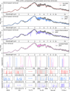 |
Fig. 4 Best-fit spectra and marginalized posterior distributions of the grid interpolation and free retrievals. First row: Exo-REM fit. Second row: ATMO fit. Third row: Sonora Diamondback fit. Fourth row: petitRADTRANS fit. Fifth row: Projected 1D posteriors for [M/H], C/O, 12C/13C, Teff, log10(g) and the radius R in the first to sixth column, respectively. For C/O, the posterior of the petitRADTRANS retrieval is shown twice because it was nominally calculated from the gas phase abundances only. For solar C/O, a ~ 25% reduction of gas phase oxygen is expected due to condensation (Sánchez-López et al. 2022), which we applied to the second, less opaque C/O posterior shown for petitRADTRANS. The last three rows show the posteriors obtained from considering the data’s 14 wavelength bands separately for the self-consistent grids, with the vertical dashed lines indicating the parameter grid values. |
4.3 Free retrievals and the case for SiO nucleation
4.3.1 Pressure-temperature profile and cloud properties
In panel a of Fig. 5 we show the retrieved pressure-temperature (P-T) distribution, while in panel b we show the logarithm of the emission contribution functions for both atmospheric columns of the winning retrieval model (i.e., spherical cloud particles of amorphous SiO). The logarithms of the contribution functions are shown instead of linear ones to make contributions other than those of thick atmospheric clouds more visible. The contribution in each column was calculated as reported in Mollière et al. (2019) (replacing the Planck function with the full scattering+emission source function), and then weighted by the wavelength-dependent flux at the top of the atmosphere, as well as the respective column coverage fractions. It can be seen that the P-T distribution shows a clear increase of temperature with pressure, such that clouds are necessary to redden the spectrum to the same degree as visible in the data (also see Fig. 3 which exhibits significant brightening in the blue wavelengths if clouds are neglected in the best-fit model). A high SiO cloud with a cloud base at ≈10−3 bar and ≈800 K in Column 1 leads to reddening of the spectra, but also produces the 10 μm absorption feature that is consistent with the MIRI MRS data. The SiO cloud is not fully opaque, however, such that most molecular features form below it, between 0.01 and 1 bar, below which (towards lower altitudes and higher pressure) a deep iron cloud cuts off emission from deeper layers. In Column 2, which only includes a Fe cloud, the atmosphere is probed at similar pressures between 0.01 and 1 bar, but somewhat less deep; here a smaller width of the log-normal particle size distribution σ leads to particles which are larger on average, leading to a stronger, approximately gray, absorption.
In panel a, we also show the P-T curves derived from the self-consistent models, here the models closest to the reported best-fit values from the species analysis. Because the grid fits all hit the lower grid boundary, we scaled their pressures by 104−log(ggrid) where log(ggrid) is the lower grid boundary. This was done to shift the photospheric location to similar pressures (Pphot ∝ g, see, e.g., Mollière et al. 2015), leading to better comparability with the pRT results which used the evolutionary prior at log(g) = 4. The grid model and the pRT temperature curves are broadly compatible, but a few noteworthy differences exist: ExoREM is colder than all other models in the high atmosphere, for (scaled) pressures <0.1 bar. Exo-REM and Sonora Diamondback both exhibit greenhouse heating due to the cloud at approximately 1 bar, which is absent in pRT. Lastly, from pressures larger than 0.3 bar, ATMO becomes very isothermal, in order to mimic the cloud spectral reddening in a cloud-free model.
In the lower row of Fig. 5, we also show the retrieved particle size distributions (panel c) and the mass fractions of the SiO and Fe clouds (panel d). We find that the SiO cloud particle size distribution peaks at ≈40 nm, such that together with the cloud deck at 10−3 bar the picture of a high-altitude small-particle SiO haze arises. The particle size distributions of the iron clouds in Columns 1 and 2 peak around 3 and 6 μm, such that this cloud species appears to grow and rain out, with a deep cloud deck at around 1 bar. Comparing the freely retrieved cloud deck locations, that is, the pressure above which the cloud is expected to disperse, to the also plotted expected onset location of condensate stability (taken from Ackerman & Marley 2001, accounting for their erratum) reveals that the retrieved iron cloud is indeed consistent with iron condensates that have settled out to the bottom of their stability region.
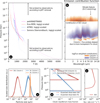 |
Fig. 5 Overview plot of the temperature, emission contribution, and cloud properties of the “winning” SiO cloud model with amorphous spherical particles, two atmospheric columns, and evolutionary priors. Panel a: retrieved pressure-temperature profiles. The pRT retrieval profile is shown in magenta. The 1–3 σ posterior regions of the temperature are indicated by progressively lighter magenta tones, but are difficult to distinguish because of the narrow posteriors. We also overplot the log10(g)-scaled P-T profiles of the grid models that are closest to the best-fit values obtained with species. Panel b: logarithmic emission contribution function of atmospheric Columns 1 and 2 as orange and purple contours. While nominally computed to sum to unity over all pressures at a given wavelength, the values have been scaled by the relative contribution of the two columns to the total atmospheric solution and multiplied by the wavelength-dependent flux. Panel c: size distribution of SiO cloud particles in Column 1 (shown in red), and Fe cloud particles in Column 1 and 2 (shown in blue and orange, respectively). For better comparability the distributions’ peak values have been normalized to the same y-axis values. The envelopes around the median distribution would correspond to the 1-σ uncertainty if the posterior variations around the median followed a Gauss distribution. Panel d: altitude-dependent cloud mass fraction of the SiO cloud (present in Column 1, shown in red) and of the Fe cloud (present in both Columns, shown in blue). The colored envelopes again represent the 1-σ uncertainty spread of the posterior distribution. The dashed lines correspond to the expected cloud deck position, obtained from intersecting the sampled P-T curves (see Panel a) with the saturation vapor pressure curves of SiO and Fe from Gail et al. (2013); Ackerman & Marley (2001). Panel e: SiO nucleation rate computed according to Gail et al. (2013). |
4.3.2 Evidence for SiO nucleation
The location of the SiO cloud is surprising. Plotting the onset location for SiO condensate stability using the saturation vapor pressure from Gail et al. (2013), we find that the SiO cloud resides at pressures which are 3 dex lower than expected (10−3 instead of 1 bar). In our implementation of the Ackerman & Marley (2001) cloud model, the cloud mass fraction would have decayed by 103fsed from 1 to 10−3 bar, if the former truly was the cloud base pressure. Instead of assuming that cloud particles are mixed from a deep cloud base to such high altitudes, we suggest that JWST probes the high-altitude formation of small SiO nuclei that seed cloud condensation. Our finding may therefore be consistent with the so-called top-down approach of cloud formation, beginning with nucleation in the upper reaches of the atmosphere (Helling et al. 2008). In general, cloud seeding nuclei are always necessary for cloud formation to ensue. This can be because the species that are expected to dominate spectra have a too high surface tension. An example is iron, which cannot form directly from the gas phase, but needs a “starting surface” (Gao et al. 2020). Another reason is that some species must form via grain-gas reactions, as in the case of the usual silicates (e.g., MgSiO3 and Mg2SiO4). Indeed, homogeneous SiO nucleation from gas-phase SiO is discussed as a likely process for triggering condensate formation, since they may then provide a surface for the other condensates to grow on Gail et al. (2013); Lee et al. (2018). SiO is the most abundant Si-bearing gas phase species, and efficiently nucleates based on predictions from thermodynamic data at the temperatures expected across the L-T transition. However, usually TiO2 is treated as the more likely nucleation species. This is because TiO2 is more refractory5 and thus nucleates before SiO in gas upwelling from the deep atmosphere. In such a situation Si would condense into silicates on the TiO2 nuclei before being able to form SiO nuclei.
However, as discussed in Lee et al. (2018), more refractory cloud nucleation species may be absent from the upper reaches of an atmosphere if the condensates in which they are incorporated rain out to low altitudes (so-called cold trapping). A likely species in the case of TiO2 would be the highly refractory calcium titanates (e.g., CaTiO3, Ca3Ti2O7, Ca4Ti3O10, see Wakeford et al. 2017). Lee et al. (2018) also argue that efficiently nucleating species may form a high-altitude haze (small particle) layer. Interestingly, when plotting the nucleation rate derived from classical nucleation theory in Gail et al. (2013) (see lower panel e in Fig. 5), we find that the peak nucleation rate is reached at 10−2 bar, so close to the retrieved SiO cloud base of 10−3 bar. For the high temperatures (T ≈ 800 > 600 K) and pressures (10−3 bar) identified for the location of the SiO cloud here, a more complete nucleation theory finds that SiO nucleation is even more efficient than predicted by classical nucleation theory (Bromley et al. 2016).
In addition, nucleation is expected to form small particles which stay aloft more easily, while larger particles would settle out of the high atmosphere more quickly (see Luna & Morley 2021, for a timescale estimate). Our inferred mean particle size of 40 nm is indeed small, but it is larger than the typical condensation nuclei made from (SiO)N clusters, which are expected to be even smaller (~nm sizes). We note, however, that constraining sizes for small particles from opacities becomes increasingly difficult, since the opacity becomes independent of particle size r in the Rayleigh limit (λ ≪ 2πr, see, e.g., Bohren & Huffman 1983). So it could be that our retrievals struggle to constrain the actual particle size, even though we do not find an upper limit (which could be related to our choice of how to parameterize the particle size distribution). In this case the remaining structure from 9.5–10 μm mentioned in Section 3.1 could be caused by the actual ro-vibrational transitions of the smallest (SiO)N clusters. Alternatively, the particles may already have grown to sizes of a few tens of nanometers when we observe them.
Lastly, we note that we did not observe evidence of absorption of SiO in the gas phase (gaseous SiO is the most important Si-bearing species prior to condensation of Si into silicates, see Visscher et al. 2010). In our retrievals it is only included as a trace species, with its abundance determined from chemical equilibrium. We do not see residuals around 8 μm, where the band head of SiO absorption lies, nor does turning the SiO gas opacity off in our best-fit model affect the fit quality noticeably.
4.3.3 Stability of atmospheric properties across retrievals
In total we have run 15 production retrievals for this study with a total computational cost of ≈106 CPU core hours (many more retrievals were run during the model development process). Their derived atmospheric bulk properties are given in Table 6. In addition to testing 11 different silicate species in our fiducial two-column model, we also tested departures from this model. Since spherical amorphous SiO particles were identified as most likely, this species was adopted for these additional retrievals. Specifically, we tested (i) turning off the evolutionary prior on the radius and log10(g), (ii) making the second column completely cloud-free, (iii) keeping the SiO and Fe cloud parameters constant across both columns but varying the temperature profile in Column 2 with the temperature excursion method, (iv) using a single-column model with an Fe and SiO cloud.
Here we discuss the stability of parameter posteriors across the different retrievals and, by extension, the likely robustness of the derived values. Such an analysis is particularly important because of the aforementioned issues with MultiNest in the present high-data-precision high-model-complexity situation. Again, robustness here is not defined as a significant overlap of retrieval posteriors for a given parameter; this is never the case, and would require that all models are sufficiently close to the optimal model or have sufficiently similar model properties. Analogous to our definition of compatibility in Section 4.2, it means that checking whether assertions such as “the metallicity is slightly super-solar, around a value of X” appear to be justified.
Before looking at the bulk parameters one-by-one, we note that the fiducial two-column model with a global iron and a patchy SiO cloud leads to the best fits consistently among all tested models (the best-fit spectra of all retrieval models are shown in Fig. C.1). In particular, the single-column model, the two P-T model, and the clear-column cloudy-column model are not favored, and are rejected with log10(B) > 100 (the log10(B) values are also given in Fig. C.1). Also the retrieval without the evolutionary prior is not favored from a BIC-based Bayes factor comparison. This is worrying as it is identical to the nominal two-column model otherwise, but more general, and should lead to a fit as least as good as the nominal model. We therefore see the aforementioned effect of MultiNest reaching its limits with the present data in classical retrieval analyses, and again caution that all results presented here should be interpreted with this finding in mind. We note that Multinest may fare better with more live points, but this is computationally unfeasible.
Effective temperature Teff. The winning model (spherical particles, amorphous SiO) constrains PSO J318’s effective temperature to ![Mathematical equation: $\[1114_{-1}^{+1}\]$](/articles/aa/full_html/2025/11/aa55732-25/aa55732-25-eq201.png) K, while the range of values seen across all retrievals ranges from 1073 to 1146 K. Given the breadth of assumptions tested in the retrievals, we may consider this parameter well constrained, with a range from 1073-1146 K.
K, while the range of values seen across all retrievals ranges from 1073 to 1146 K. Given the breadth of assumptions tested in the retrievals, we may consider this parameter well constrained, with a range from 1073-1146 K.
Radius R. The winning model constrains the radius to ![Mathematical equation: $\[1.495_{-0.007}^{+0.007}\]$](/articles/aa/full_html/2025/11/aa55732-25/aa55732-25-eq202.png) RJup, with the retrievals ranging from 1.454 to 1.516 RJup in the cases with the evolutionary prior, 𝒩(1.36 RJup, 0.09 RJup). This is not too far from the result obtained when turning off the evolutionary prior, which is
RJup, with the retrievals ranging from 1.454 to 1.516 RJup in the cases with the evolutionary prior, 𝒩(1.36 RJup, 0.09 RJup). This is not too far from the result obtained when turning off the evolutionary prior, which is ![Mathematical equation: $\[1.54_{-0.01}^{+0.02}\]$](/articles/aa/full_html/2025/11/aa55732-25/aa55732-25-eq203.png) RJup. This parameter may therefore be considered robust, yielding a radius value of around 1.5 RJup.
RJup. This parameter may therefore be considered robust, yielding a radius value of around 1.5 RJup.
Luminosity L. The winning model constrains the bolometric luminosity to log(L/L⊙) = ![Mathematical equation: $\[-4.489_{-0.005}^{+0.003}\]$](/articles/aa/full_html/2025/11/aa55732-25/aa55732-25-eq204.png) , with the retrievals ranging from −4.532 to −4.441 L⊙, which makes for a robust determination of this parameter. This value range is somewhat lower than, but consistent with, the log(L/L⊙) = −4.420 ± 0.060 quoted in Zhang et al. (2020), which was derived based on NIR photometry.
, with the retrievals ranging from −4.532 to −4.441 L⊙, which makes for a robust determination of this parameter. This value range is somewhat lower than, but consistent with, the log(L/L⊙) = −4.420 ± 0.060 quoted in Zhang et al. (2020), which was derived based on NIR photometry.
Gravity log10(g). The winning model constrains the atmospheric gravity to ![Mathematical equation: $\[4.009_{-0.007}^{+0.007}\]$](/articles/aa/full_html/2025/11/aa55732-25/aa55732-25-eq205.png) , with most retrievals falling close to that range, which is determined by the adopted prior, 𝒩(4, 0.04). If this prior is turned off and a uniform prior is adopted instead, the retrieval runs into the lower boundary of the prior (log10(g) = 3), similar to the grid fits with the self-consistent models. We therefore conclude that this parameter is not robust for the data considered here, and that medium- to high-resolution observations in the NIR may lead to a better constraint, as discussed in Section 4.1. Alternatively, running the JWST retrievals at full, or at least higher, resolution may be beneficial; the JWST MIRI studies of WISE J1828 (Barrado et al. 2023), WISE J0855 (Kühnle et al. 2025), and WISE J0458 (Matthews et al. 2025) all ran retrievals at λ/Δλ = 1000 for MRS and resulted in bounded constraints. We again note that turning off the evolutionary prior led to a significantly worse fit. This demonstrates how the struggling nested sampling benefits from the use of informative priors, especially on log10(g).
, with most retrievals falling close to that range, which is determined by the adopted prior, 𝒩(4, 0.04). If this prior is turned off and a uniform prior is adopted instead, the retrieval runs into the lower boundary of the prior (log10(g) = 3), similar to the grid fits with the self-consistent models. We therefore conclude that this parameter is not robust for the data considered here, and that medium- to high-resolution observations in the NIR may lead to a better constraint, as discussed in Section 4.1. Alternatively, running the JWST retrievals at full, or at least higher, resolution may be beneficial; the JWST MIRI studies of WISE J1828 (Barrado et al. 2023), WISE J0855 (Kühnle et al. 2025), and WISE J0458 (Matthews et al. 2025) all ran retrievals at λ/Δλ = 1000 for MRS and resulted in bounded constraints. We again note that turning off the evolutionary prior led to a significantly worse fit. This demonstrates how the struggling nested sampling benefits from the use of informative priors, especially on log10(g).
Column coverage B. While the winning model shows clear evidence of a two-column solution being favored (B = 0.695 ± 0.002, where the Bs of HST, SpeX and JWST were averaged), some other models, for example the glassy MgSiO3 cases, do not require a 1+1D structure to result in a decent fit. We note, however, that these models still lead to a worse fit, and are disfavored with log10(B) = 32.18, using the BIC-to-evidence conversion method. We note that the glassy MgSiO3 cases in particular lead to residuals in the 4 μm emission peak, see Fig. C.1.
Metallicity [M/H]. The winning model constrains the atmospheric metallicity to be slightly super-solar, at ![Mathematical equation: $\[0.31_{-0.01}^{+0.01}\]$](/articles/aa/full_html/2025/11/aa55732-25/aa55732-25-eq206.png) . The values observed for the various retrievals range from 0.12 to 0.6, such that the claim of a slightly super-solar metallicity appears to be justified, but the exact degree of enrichment is less straightforward to constrain.
. The values observed for the various retrievals range from 0.12 to 0.6, such that the claim of a slightly super-solar metallicity appears to be justified, but the exact degree of enrichment is less straightforward to constrain.
Carbon-to-oxygen number ratio C/O. The retrieved C/O values are largely consistent across the retrievals. The winning model constrains C/O to ![Mathematical equation: $\[0.789_{-0.003}^{+0.003}\]$](/articles/aa/full_html/2025/11/aa55732-25/aa55732-25-eq207.png) , and the highest value seen across all runs goes up to 0.872. Applying the aforementioned 25% oxygen correction to account for its sequestration into silicates leads to a range from 0.580 to 0.654, so slightly super-solar when compared to Asplund et al. (2009), who find C/O = 0.55 for the sun.
, and the highest value seen across all runs goes up to 0.872. Applying the aforementioned 25% oxygen correction to account for its sequestration into silicates leads to a range from 0.580 to 0.654, so slightly super-solar when compared to Asplund et al. (2009), who find C/O = 0.55 for the sun.
Carbon isotope ratio 12C/13C. In the retrievals, the abundances of 13CO and 12CO are treated independently, which allows testing for the presence of 13CO and measuring of its abundance in PSO J318. This is motivated by Gandhi et al. (2023), who identified 12CO, 13CO, C17O and C18O using NIRSpec G395H in the atmosphere of VHS 1256b, which is a similar object. 13CO is likely the easiest secondary isotopologue to detect in atmospheres of substellar objects hot enough to exhibit appreciable CO absorption (Mollière & Snellen 2019; Zhang et al. 2021). However, isotopologues are not the main focus of this study, and NIRSpec G395H NRS2 has been binned to λ/Δλ = 1000 in our work (while its intrinsic resolution is R ≈ 3200 from 4–5 μm). This means that the minute changes of the individual lines of rarer isotopologues are harder to pick up. Therefore we did not search for the less abundant C17O and C18O isotopologues. The winning pRT model detects 13CO, and constrains 12C/13C ≈ 12CO/13CO = ![Mathematical equation: $\[45_{-4}^{+5}\]$](/articles/aa/full_html/2025/11/aa55732-25/aa55732-25-eq208.png) . Across the retrievals this value varies quite substantially (from 17 to 81 for the retrievals with bounded constraints). These value are generally lower than the local value of 70 in the interstellar medium (Milam et al. 2005), which is surprising for an isolated object that may represent the low-mass end of star formation. To understand these constraints better we show a zoomed in version of PSO J318’s spectrum in the 4–5 μm region, at the full resolution of G 395 H NRS2, in Fig. 6. We also show the best-fit model of pRT, post-processed to high spectral resolution λ/Δλ = 250 000, convolved to R = 3200, binned to the G395H NRS2 wavelength solution and then superimposed on the PSO J318 data. The fit is decent, but residuals between the data and model persist. In particular, the PSO J318 data appears to be noisier and still affected by systematic effects when compared to the corresponding spectrum of VHS 1256b (Miles et al. 2023), which we also show in the same panel. Even though the retrieval was run on the PSO J318 and not the VHS 1256b data, the latter are better fit by the retrieval model. In the right panels we show a further zoomed-in view of the PSO J318 data, together with the best-fit pRT model with and without considering the 13CO opacity. We conclude that while 13CO lines are clearly visible in the spectrum of PSO J318, noise and remaining systematic effects in the data might currently hinder an accurate determination of 12C/13C (we note again that we use the standard reduction for G395H from the MAST archive for PSO J318).
. Across the retrievals this value varies quite substantially (from 17 to 81 for the retrievals with bounded constraints). These value are generally lower than the local value of 70 in the interstellar medium (Milam et al. 2005), which is surprising for an isolated object that may represent the low-mass end of star formation. To understand these constraints better we show a zoomed in version of PSO J318’s spectrum in the 4–5 μm region, at the full resolution of G 395 H NRS2, in Fig. 6. We also show the best-fit model of pRT, post-processed to high spectral resolution λ/Δλ = 250 000, convolved to R = 3200, binned to the G395H NRS2 wavelength solution and then superimposed on the PSO J318 data. The fit is decent, but residuals between the data and model persist. In particular, the PSO J318 data appears to be noisier and still affected by systematic effects when compared to the corresponding spectrum of VHS 1256b (Miles et al. 2023), which we also show in the same panel. Even though the retrieval was run on the PSO J318 and not the VHS 1256b data, the latter are better fit by the retrieval model. In the right panels we show a further zoomed-in view of the PSO J318 data, together with the best-fit pRT model with and without considering the 13CO opacity. We conclude that while 13CO lines are clearly visible in the spectrum of PSO J318, noise and remaining systematic effects in the data might currently hinder an accurate determination of 12C/13C (we note again that we use the standard reduction for G395H from the MAST archive for PSO J318).
PSO J318 retrieval results.
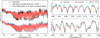 |
Fig. 6 Evidence of 13CO absorption in PSO J318’s atmosphere. Left panel: best-fit spectrum of the winning pRT retrieval model (amorphous spherical SiO particles) post-processed to high spectral resolution (R = 3200, red solid line) and superimposed on the NIRSpec G395H NRS2 data of PSO J318 at full spectral resolution (black solid line). For comparison, pRT’s best-fit model for PSO J318 is also superimposed on a scaled version of VHS 1256b’s G395H spectrum from Miles et al. (2023) (blue solid line). Right panel: zoomed-in version of the left panel showing the data for PSO J318 as well as the pRT best-fit model, where in one case (cyan solid line) the 13CO opacity has been turned off in post-processing. |
5 Summary and discussion
In this work, we have analyzed the panchromatic emission spectrum of the young low-mass brown dwarf PSO J318, a “rogue planet”. We considered data from 1–18 μm taken with JWST NIRSpec and MIRI observations together with archival HST and IRTF SpeX spectra. We summarize our findings below:
The emission of PSO J318 is extremely red and exhibits a broad and deep absorption feature at 10 μm, which we attribute to absorption by silicate clouds;
We developed a technique to efficiently identify likely cloud species based on the wavelength-dependent brightness temperature of PSO J318. This method suggests that the absorption is caused by spherical amorphous SiO grains. This prediction agrees with the subsequently run retrievals;
Starting from the list of silicate species identified with the brightness temperature method, we ran full retrievals on the spectra with petitRADTRANS. We find satisfactory fits to the data across the full spectral range. These retrievals also identify SiO as the most likely species, strongly favoring it over other candidates when using BIC-derived Bayes factors;
We hypothesize that our observations probe the homogeneous nucleation of SiO cloud seeds from the gas phase, which is consistent with the high altitude retrieved for the cloud base (≈1 mbar), and the small particle sizes ≲0.1 μm. These particles could then provide the surfaces required for cloud formation at lower altitudes;
Our retrievals indicate that PSO J318 may be best described by atmospheres more complex than what can be described by a 1D column. Our favored models describe the atmosphere in a 1+1D column approach. These two columns have a global Fe cloud, but only one column hosts a silicate cloud. While this need for a more than 1D solution is consistent with the reported variability of PSO J318, it does not perfectly reproduce its observed variability behavior (Biller et al. 2018). The silicate cloud coverage of the winning SiO model is 0.695 when averaged over the epochs of the three observatories (HST, SpeX, JWST). The coverage of the three instruments, when compared to this mean, varies by ~±4%. Taking this as a typical value of the expected coverage variability, we can roughly reproduce the similar relative variability amplitudes observed between HST and SpeX wavelengths. However, while they are in phase for our models, they are phase shifted by 200° in Biller et al. (2018). What is more, the variability reported in Biller et al. (2018) is gray across the HST wavelengths, which is not what we find. This could indicate that more than two columns are necessary to explain PSO J318’s variability and that more quantities than the silicate cloud cover could vary, consistent with the qualitative interpretation of JWST variability data in Biller et al. (2024); McCarthy et al. (2025); Chen et al. (2025);
Our retrievals also indicate that solutions that vary the temperature structure across two columns but assume identical cloud properties across the two columns are not favored when compared to our fiducial two column model. So a temperature-profile induced reddening of the spectra as suggested by Tremblin et al. (2015, 2016, 2017, 2019) is not supported by the results obtained with our current retrieval setup;
We also ran grid retrievals using various atmospheric models in radiative-convective equilibrium (Exo-REM, ATMO, Sonora Diamondback). The retrieved bulk properties between these self-consistent models and the petitRADTRANS retrievals are mutually compatible, while the small posterior uncertainties make them mutually inconsistent. Compatibility here means that we find that PSO J318 is slightly enriched in metals when compared to solar across the various approaches, with potentially a solar to a slightly super-solar C/O. The atmospheric gravity cannot be constrained from the data: All self-consistent model grids hit the lower grid boundary, and petitRADTRANS only achieves a bound value on log10(g) if an evolutionary prior is used. This could potentially be alleviated by adding (existing) NIR observations at higher spectral resolution to the analysis or by considering the JWST data at full (or higher) resolution. The latter were binned down in the present analysis in order to make running the retrievals feasible (they still took ~105 CPU core hours per run);
In general, the self-consistent models struggle to achieve a satisfactory fit across the full wavelength range, pointing to the need of an improved description (or parameterization) of atmospheric mixing in connection to disequilibrium chemistry and an improved treatment of the deep iron cloud and the high-altitude silicate cloud that produces the 10 μm feature. Exploring a more than 1D approach in self-consistent models may also be beneficial;
We observed that our retrievals struggle to converge to the best-fit parameter values, or converge at all, at times. For example, removing the evolutionary prior on log10(g) and radius in an otherwise identical retrieval leads to a worse fit. This shows that techniques such as nested sampling reach their limit in the JWST era of high-precision data with wide wavelength coverage, which also require more complex (≳40 free parameters) models. This problem is also relevant with respect to the imminent first light of the ELT, slated for the early 2030s, from which we will get high S/N data at high spectral resolution and wide wavelength coverage.
We note here that the presence of high-altitude small SiO cloud particles has also been inferred in the work of Luna & Morley (2021); Suárez & Metchev (2023). Suárez & Metchev (2023) reported that small SiO (or MgSiO3) particles high in the atmosphere appear to be most prevalently occurring for high-gravity (log10(g) > 5) L-dwarfs since small particles are the only ones that may stay aloft. In contrast, they found that larger (~1 μm) pyroxene-type (MgxFe1−xSiO3) grains may be present in the high atmosphere for lower gravity objects (log 10(g) ≲ 4.5). For PSO J318, we find that SiO would still have to be mixed up across 3 dex in pressure from its thermo-chemically expected cloud base to be visible, which may be unlikely. Additionally, if it is indeed SiO particles that are visible in the spectra, mixing from low altitudes to high in the atmosphere would be challenging, as SiO is not chemically favored if produced by condensation (rather than nucleation). We therefore argue that it is not mixing that keeps the small particles aloft in PSO J318. Instead we posit that the SiO particles nucleate locally, which is consistent with the so-called top-down cloud formation approach (Helling et al. 2008). Indeed, our actually inferred location of the SiO cloud coincides with the expected location of maximum SiO nucleation (Gail et al. 2013). What is more, PSO J318 is a known planetary-mass object, which is inconsistent with the log10(g) trend identified in Suárez & Metchev (2023). More retrieval work for a set of objects spanning a large log10(g) and temperature range is required to understand the behavior of these clouds better.
Some example spectra of brown dwarfs and low-mass companions are shown in Fig. 7 in comparison to the flux observed for PSO J318. In the figure, we plot VHS 1256-1257b (spectral type L7±1.5, Miles et al. 2023), 2MASS J1821+1414 (L4.5/L5p, Suárez & Metchev 2022), YSES-1c (L7.5, Hoch et al. 2025), and 2MASS J1507-1627 (L5/L5.5, Suárez & Metchev 2022). Some objects appear to be consistent with the flux of PSO J318, especially VHS 1256b and 2MASS J1821+1414, but the properties of these objects and the ones that look different (here YSES-1c and 2MASS J1507-1627) should be studied more carefully. Interestingly, the potential preference for SiO in 2MASS J1821+1414 has been reported in the aforementioned work Luna & Morley (2021), while those authors also report a preference for Mg2SiO4 and MgSiO3 for 2MASS J1507-1627. For YSES-1c, a combination of amorphous MgSiO3 and Mg2SiO4 is cited as explaining the feature well, or, alternatively, iron-enriched silicates (Hoch et al. 2025). This would be consistent with the redder onset of the silicate feature. If SiO nucleation is prevalent in at least some classes of directly imaged planets and brown dwarfs, it may also explain why the 10 μm feature appears to be often best described by amorphous silicate absorption: While to this day the actual structure of SiO evades us (see Brady 1959; Philipp 1971, for the still relevant models), it is generally accepted that condensed SiO is highly amorphous (Hass 1950; Schnurre et al. 2004).
Any retrieval analyses of such objects would benefit from being backed up by dedicated microphysical cloud models that incorporate not only the nucleation of species such as SiO and TiO2 but also model the condensation, settling, and mixing of silicate species such as MgSiO3 or Mg2SiO4 as well as gas-grain reactions (e.g., SiO should oxidize to SiO2 quite quickly). If SiO nuclei are present, it should also be investigated why only they are visible and not the cloud species that are expected to condense on them. SiO nuclei could form more efficiently than the expected condensation of the “usual” silicate species (MgSiO3, Mg2SiO4, ...) on their surfaces, or more efficiently than their expected oxidization into SiO2.
We also find that the retrieval community is in need of improved inference techniques that speed up and enhance the robustness of retrievals. We are facing the “no free lunch” theorem, as we cannot significantly change the properties of our data (wider wavelength coverage, significantly better signal to noise) and the type of questions we ask (e.g., whether the atmosphere is multi-dimensional) and expect our classical inference algorithms to still work. Separating the data into wavelength sections that allow us to ask questions that are independently answerable could be one approach to address this problem, such as we did here with the brightness temperature method. Another example is the work by Gandhi et al. (2023), who only used NIRSpec G395H data to measure CO isotopologue abundances in VHS 1256b. Alternatively, a promising avenue is exploring the usefulness of machine learning inference approaches, such as amortized or sequential simulation-based inference (Cranmer et al. 2020), for which early work for exoplanet and brown dwarf atmospheres exist (Vasist et al. 2023; Barrado et al. 2023; Ardévol Martínez et al. 2024; Lueber et al. 2025) but which have not yet been applied to models as complex (in terms of number of parameters) as the ones we employed here.
If such improved inference methods can be developed to run efficiently on the data investigated here, the suggested SiO detection from this work should be revisited to explore the robustness of our finding. There are other runners-up for the most likely cloud species, such as glassy amorphous MgSiO3, which lead to a good (but worse) fit. The properties of the silicate cloud should thus be studied by exploring a wider range of forward model setups. The current numerical cost of the retrievals makes this inefficient. Relatedly, such methods would potentially also enable study of the variability of objects such as PSO J318 in more detail. Data sets that record the evolution of spectra over multiple rotational periods now exist (Biller et al. 2024; McCarthy et al. 2025; Chen et al. 2025), but it will be challenging to develop retrieval approaches that can take the full information content of these data into account.
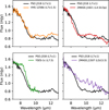 |
Fig. 7 Comparison between the 10μm flux of PSO J318 and the (scaled) flux of brown dwarfs and low-mass companions with mid-L and L-T transition spectral types. |
Acknowledgements
P.M. thanks the referee, Caroline Morley, for a careful and constructive review of the paper. P.M. would also like to thank the editor Emmanuel Lellouch for additional comments on the manuscript. In addition, P.M. thanks Laura Kreidberg, Evert Nasedkin, and Johanna Vos for insightful discussions which improved the quality of the paper. This work is based (in part) on observations made with the NASA/ESA/CSA James Webb Space Telescope. The data were obtained from the Mikulski Archive for Space Telescopes at the Space Telescope Science Institute, which is operated by the Association of Universities for Research in Astronomy, Inc., under NASA contract NAS 5-03127 for JWST. These observations are associated with program #1275. All the JWST data used in this paper can be found in MAST under the DOI 10.17909/2y71-fq23. The following National and International Funding Agencies funded and supported the development of JWST’s MIRI instrument, which was used in this work: NASA; ESA; Belgian Science Policy Office (BELSPO); Centre Nationale d’Etudes Spatiales (CNES); Danish National Space Centre; Deutsches Zentrum fur Luft und Raumfahrt (DLR); Enterprise Ireland; Ministerio De Economıa y Competividad; Netherlands Research School for Astronomy (NOVA); Netherlands Organisation for Scientific Research (NWO); Science and Technology Facilities Council; Swiss Space Office; Swedish National Space Agency; and UK Space Agency. P-O.L. acknowledges funding support by CNES. Z.Z. acknowledges the support of the NASA Hubble Fellowship grant HST-HF2-51522.001-A. P.P. thanks the Swiss National Science Foundation (SNSF) for financial support under grant number 200020_200399. L.D. acknowledges funding support from the KU Leuven Interdisciplinary Grant (IDN/19/028), the European Union H2020-MSCA-ITN-2019 under Grant no. 860470 (CHAMELEON) and the FWO research grant G086217N. B.A.B. acknowledges funding by the UK Science and Technology Facilities Council (STFC) grant no. ST/V000594/1. O.A. is a Senior Research Associate of the Fonds de la Recherche Scientifique – FNRS. This project has received funding from the European Research Council (ERC) under the European Union’s Horizon 2020 research and innovation programme (grant agreement No 819155). I.A. would like to thank the European Space Agency (ESA) and the Belgian Federal Science Policy Office (BELSPO) for their support in the framework of the PRODEX Programme. DB is funded by grant PID2023-150468NB-I00 by the Spanish Ministry of Science and Innovation/State Agency of Research MCIN/AEI/10.13039/501100011033. JPP acknowledges financial support from the UK Science and Technology Facilities Council, and the UK Space Agency. M.S. acknowledges support from the European Research Council under the Horizon 2020 Framework Program via the ERC Advanced Grant Origins 83 24 28. N.W. acknowledges support from NSF award #2238468, #1909776, and NASA Award #80NSSC22K0142. EvD acknowledges support from A-ERC grant 101019751 MOLDISK. G.Ö. acknowledges support from the Swedish National Space Agency (SNSA).
References
- Ackerman, A. S., & Marley, M. S. 2001, ApJ, 556, 872 [Google Scholar]
- Allard, F., Hauschildt, P. H., Alexander, D. R., Tamanai, A., & Schweitzer, A. 2001, ApJ, 556, 357 [Google Scholar]
- Allard, N. F., Spiegelman, F., Leininger, T., & Molliere, P. 2019, A&A, 628, A120 [NASA ADS] [CrossRef] [EDP Sciences] [Google Scholar]
- Allers, K. N., & Liu, M. C. 2013, ApJ, 772, 79 [NASA ADS] [CrossRef] [Google Scholar]
- Allers, K. N., Gallimore, J. F., Liu, M. C., & Dupuy, T. J. 2016, ApJ, 819, 133 [Google Scholar]
- Apai, D., Radigan, J., Buenzli, E., et al. 2013, ApJ, 768, 121 [NASA ADS] [CrossRef] [Google Scholar]
- Ardévol Martínez, F., Min, M., Huppenkothen, D., Kamp, I., & Palmer, P. I. 2024, A&A, 681, L14 [NASA ADS] [CrossRef] [EDP Sciences] [Google Scholar]
- Asplund, M., Grevesse, N., Sauval, A. J., & Scott, P. 2009, ARA&A, 47, 481 [NASA ADS] [CrossRef] [Google Scholar]
- Azzam, A. A. A., Tennyson, J., Yurchenko, S. N., & Naumenko, O. V. 2016, MNRAS, 460, 4063 [NASA ADS] [CrossRef] [Google Scholar]
- Barber, R. J., Strange, J. K., Hill, C., et al. 2013, MNRAS, 437, 1828 [Google Scholar]
- Barrado, D., Mollière, P., Patapis, P., et al. 2023, Nature, 624, 263 [NASA ADS] [CrossRef] [Google Scholar]
- Barrado y Navascués, D., Stauffer, J. R., Song, I., & Caillault, J. P. 1999, ApJ, 520, L123 [CrossRef] [Google Scholar]
- Baudino, J.-L., Bézard, B., Boccaletti, A., et al. 2015, A&A, 582, A83 [NASA ADS] [CrossRef] [EDP Sciences] [Google Scholar]
- Benneke, B., & Seager, S. 2013, ApJ, 778, 153 [Google Scholar]
- Biller, B. 2017, Astron. Rev., 13, 1 [Google Scholar]
- Biller, B. A., Vos, J., Bonavita, M., et al. 2015, ApJ, 813, L23 [Google Scholar]
- Biller, B. A., Vos, J., Buenzli, E., et al. 2018, AJ, 155, 95 [NASA ADS] [CrossRef] [Google Scholar]
- Biller, B. A., Vos, J. M., Zhou, Y., et al. 2024, MNRAS, 532, 2207 [NASA ADS] [CrossRef] [Google Scholar]
- Blain, D., Charnay, B., & Bézard, B. 2021, A&A, 646, A15 [EDP Sciences] [Google Scholar]
- Blain, D., Mollière, P., & Nasedkin, E. 2024, J. Open Source Softw., 9, 7028 [Google Scholar]
- Bodenheimer, P., D’Angelo, G., Lissauer, J. J., Fortney, J. J., & Saumon, D. 2013, ApJ, 770, 120 [NASA ADS] [CrossRef] [Google Scholar]
- Bohren, C. F., & Huffman, D. R. 1983, Absorption and Scattering of Light by Small Particles [Google Scholar]
- Bouwman, J., Meeus, G., de Koter, A., et al. 2001, A&A, 375, 950 [NASA ADS] [CrossRef] [EDP Sciences] [Google Scholar]
- Brady, G. W. 1959, J. Phys. Chem., 63, 1119 [Google Scholar]
- Bromley, S. T., Gómez Martín, J. C., & Plane, J. M. C. 2016, Phys. Chem. Chem. Phys., 18, 26913 [NASA ADS] [CrossRef] [Google Scholar]
- Buchner, J. 2023, Statist. Surv., 17, 169 [NASA ADS] [CrossRef] [Google Scholar]
- Buchner, J., Georgakakis, A., Nandra, K., et al. 2014, A&A, 564, A125 [NASA ADS] [CrossRef] [EDP Sciences] [Google Scholar]
- Burningham, B., Faherty, J. K., Gonzales, E. C., et al. 2021, MNRAS, 506, 1944 [NASA ADS] [CrossRef] [Google Scholar]
- Burrows, A., Marley, M., Hubbard, W. B., et al. 1997, ApJ, 491, 856 [Google Scholar]
- Burrows, A., Ram, R. S., Bernath, P., Sharp, C. M., & Milsom, J. A. 2002, ApJ, 577, 986 [NASA ADS] [CrossRef] [Google Scholar]
- Bushouse, H., Eisenhamer, J., Dencheva, N., et al. 2023, JWST Calibration Pipeline [Google Scholar]
- Calamari, E., Faherty, J. K., Visscher, C., et al. 2024, ApJ, 963, 67 [NASA ADS] [CrossRef] [Google Scholar]
- Campos Estrada, B., Lewis, D. A., Helling, C., et al. 2025, A&A, 694, A275 [NASA ADS] [CrossRef] [EDP Sciences] [Google Scholar]
- Chabrier, G., Johansen, A., Janson, M., & Rafikov, R. 2014, in Protostars and Planets VI, eds. H. Beuther, R. S. Klessen, C. P. Dullemond, & T. Henning, 619 [Google Scholar]
- Charnay, B., Bézard, B., Baudino, J. L., et al. 2018, ApJ, 854, 172 [Google Scholar]
- Chen, X., Biller, B. A., Tan, X., et al. 2025, MNRAS, 539, 3758 [Google Scholar]
- Chubb, K. L., & Min, M. 2022, A&A, 665, A2 [NASA ADS] [CrossRef] [EDP Sciences] [Google Scholar]
- Chubb, K. L., Rocchetto, M., Yurchenko, S. N., et al. 2021, A&A, 646, A21 [NASA ADS] [CrossRef] [EDP Sciences] [Google Scholar]
- Coles, P. A., Yurchenko, S. N., & Tennyson, J. 2019, MNRAS, 490, 4638 [CrossRef] [Google Scholar]
- Cranmer, K., Brehmer, J., & Louppe, G. 2020, PNAS, 117, 30055 [NASA ADS] [CrossRef] [Google Scholar]
- Cushing, M. C., Roellig, T. L., Marley, M. S., et al. 2006, ApJ, 648, 614 [Google Scholar]
- Dittmann, A. 2024, Open J. Astrophys., 7, 79 [Google Scholar]
- Dorschner, J., Begemann, B., Henning, T., Jaeger, C., & Mutschke, H. 1995, A&A, 300, 503 [Google Scholar]
- Draine, B. T. 1988, ApJ, 333, 848 [NASA ADS] [CrossRef] [Google Scholar]
- Dyrek, A., Min, M., Decin, L., et al. 2024, Nature, 625, 51 [Google Scholar]
- Fabian, D., Jäger, C., Henning, T., Dorschner, J., & Mutschke, H. 2000, A&A, 364, 282 [Google Scholar]
- Fabian, D., Henning, T., Jäger, C., et al. 2001, A&A, 378, 228 [NASA ADS] [CrossRef] [EDP Sciences] [Google Scholar]
- Faherty, J. K. 2018, Spectral Properties of Brown Dwarfs and Unbound Planetary Mass Objects, 188 [Google Scholar]
- Feroz, F., & Hobson, M. P. 2008, MNRAS, 384, 449 [NASA ADS] [CrossRef] [Google Scholar]
- Feroz, F., Hobson, M. P., & Bridges, M. 2009, MNRAS, 398, 1601 [NASA ADS] [CrossRef] [Google Scholar]
- Feroz, F., Hobson, M. P., Cameron, E., & Pettitt, A. N. 2019, Open J. Astrophys., 2, 10 [Google Scholar]
- Gail, H.-P. 2001, A&A, 378, 192 [NASA ADS] [CrossRef] [EDP Sciences] [Google Scholar]
- Gail, H.-P. 2004, A&A, 413, 571 [NASA ADS] [CrossRef] [EDP Sciences] [Google Scholar]
- Gail, H.-P. 2010, Astromineralogy, 815, ed. T. Henning (Springer) [Google Scholar]
- Gail, H. P., Wetzel, S., Pucci, A., & Tamanai, A. 2013, A&A, 555, A119 [NASA ADS] [CrossRef] [EDP Sciences] [Google Scholar]
- Gandhi, S., de Regt, S., Snellen, I., et al. 2023, ApJ, 957, L36 [NASA ADS] [CrossRef] [Google Scholar]
- Gao, P., Marley, M. S., & Ackerman, A. S. 2018, ApJ, 855, 86 [Google Scholar]
- Gao, P., Thorngren, D. P., Lee, G. K. H., et al. 2020, Nat. Astron., 4, 951 [NASA ADS] [CrossRef] [Google Scholar]
- Gardner, J. P., Mather, J. C., Abbott, R., et al. 2023, PASP, 135, 068001 [NASA ADS] [CrossRef] [Google Scholar]
- Grant, D., Lewis, N. K., Wakeford, H. R., et al. 2023, ApJ, 956, L32 [NASA ADS] [CrossRef] [Google Scholar]
- Hansen, J. E. 1971, J. Atmos. Sci., 28, 1400 [NASA ADS] [CrossRef] [Google Scholar]
- Hargreaves, R. J., Gordon, I. E., Rey, M., et al. 2020, ApJS, 247, 55 [NASA ADS] [CrossRef] [Google Scholar]
- Harker, D. E., & Desch, S. J. 2002, ApJ, 565, L109 [NASA ADS] [CrossRef] [Google Scholar]
- Hass, G. 1950, J. Am. Ceram. Soc., 33, 353 [Google Scholar]
- Helling, C., Woitke, P., & Thi, W. F. 2008, A&A, 485, 547 [NASA ADS] [CrossRef] [EDP Sciences] [Google Scholar]
- Henning, T. 2010, ARA&A, 48, 21 [Google Scholar]
- Henning, T., & Stognienko, R. 1993, A&A, 280, 609 [Google Scholar]
- Henning, T., & Mutschke, H. 1997, A&A, 327, 743 [NASA ADS] [Google Scholar]
- Himes, M. 2022, PhD thesis, University of Central Florida, doctoral Dissertation (Open Access) [Google Scholar]
- Hoch, K. K. W., Rowland, M., Petrus, S., et al. 2025, Nature, 643, 938 [Google Scholar]
- Hubeny, I. 2017, MNRAS, 469, 841 [NASA ADS] [CrossRef] [Google Scholar]
- Inglis, J., Batalha, N. E., Lewis, N. K., et al. 2024, ApJ, 973, L41 [NASA ADS] [CrossRef] [Google Scholar]
- Jaeger, C., Molster, F. J., Dorschner, J., et al. 1998, A&A, 339, 904 [Google Scholar]
- Jäger, C., Mutschke, H., Begemann, B., Dorschner, J., & Henning, T. 1994, A&A, 292, 641 [NASA ADS] [Google Scholar]
- Jäger, C., Dorschner, J., Mutschke, H., Posch, T., & Henning, T. 2003a, A&A, 408, 193 [NASA ADS] [CrossRef] [EDP Sciences] [Google Scholar]
- Jäger, C., Il’in, V. B., Henning, T., et al. 2003b, J. Quant. Spec. Radiat. Transf., 79, 765 [Google Scholar]
- Jakobsen, P., Ferruit, P., Alves de Oliveira, C., et al. 2022, A&A, 661, A80 [NASA ADS] [CrossRef] [EDP Sciences] [Google Scholar]
- Juhász, A., Bouwman, J., Henning, T., et al. 2010, ApJ, 721, 431 [Google Scholar]
- Kiefer, S., Samra, D., Lewis, D. A., et al. 2024, A&A, 690, A244 [NASA ADS] [CrossRef] [EDP Sciences] [Google Scholar]
- Kipping, D., & Benneke, B. 2025, arXiv e-prints [arXiv:2506.05392] [Google Scholar]
- Kitzmann, D., & Heng, K. 2018, MNRAS, 475, 94 [NASA ADS] [CrossRef] [Google Scholar]
- Koike, C., Kaito, C., Yamamoto, T., et al. 1995, Icarus, 114, 203 [NASA ADS] [CrossRef] [Google Scholar]
- Koike, C., Mutschke, H., Suto, H., et al. 2006, A&A, 449, 583 [CrossRef] [EDP Sciences] [Google Scholar]
- Kühnle, H., Patapis, P., Mollière, P., et al. 2025, A&A, 695, A224 [NASA ADS] [CrossRef] [EDP Sciences] [Google Scholar]
- Law, D. R., Morrison, J. E., Argyriou, I., et al. 2023, AJ, 166, 45 [NASA ADS] [CrossRef] [Google Scholar]
- Leconte, J. 2021, A&A, 645, A20 [NASA ADS] [CrossRef] [EDP Sciences] [Google Scholar]
- Lee, E. K. H., Blecic, J., & Helling, C. 2018, A&A, 614, A126 [NASA ADS] [CrossRef] [EDP Sciences] [Google Scholar]
- Lei, E., & Mollière, P. 2024, arXiv e-prints [arXiv:2410.21364] [Google Scholar]
- Lew, B. W. P., Apai, D., Marley, M., et al. 2020, ApJ, 903, 15 [NASA ADS] [CrossRef] [Google Scholar]
- Line, M. R., Teske, J., Burningham, B., Fortney, J. J., & Marley, M. S. 2015, ApJ, 807, 183 [NASA ADS] [CrossRef] [Google Scholar]
- Line, M. R., Marley, M. S., Liu, M. C., et al. 2017, ApJ, 848, 83 [NASA ADS] [CrossRef] [Google Scholar]
- Liu, M. C., Magnier, E. A., Deacon, N. R., et al. 2013, ApJ, 777, L20 [NASA ADS] [CrossRef] [Google Scholar]
- Lueber, A., Karchev, K., Fisher, C., et al. 2025, ApJ, 984, L32 [Google Scholar]
- Luna, J. L., & Morley, C. V. 2021, ApJ, 920, 146 [NASA ADS] [CrossRef] [Google Scholar]
- MacDonald, R. J., & Batalha, N. E. 2023, RNAAS, 7, 54 [NASA ADS] [Google Scholar]
- Madhusudhan, N. 2018, Atmospheric Retrieval of Exoplanets, eds. H. J. Deeg, & J. A. Belmonte (Cham: Springer International Publishing), 2153 [Google Scholar]
- Madhusudhan, N., Amin, M. A., & Kennedy, G. M. 2014, ApJ, 794, L12 [Google Scholar]
- Mamajek, E. E., & Bell, C. P. M. 2014, MNRAS, 445, 2169 [Google Scholar]
- Marley, M. S., & Robinson, T. D. 2015, ARA&A, 53, 279 [Google Scholar]
- Matthews, E. C., Mollière, P., Kühnle, H., et al. 2025, ApJ, 981, L31 [Google Scholar]
- McCarthy, A. M., Vos, J. M., Muirhead, P. S., et al. 2025, ApJ, 981, L22 [Google Scholar]
- McKemmish, L. K., Masseron, T., Hoeijmakers, H. J., et al. 2019, MNRAS, 488, 2836 [Google Scholar]
- Milam, S. N., Savage, C., Brewster, M. A., Ziurys, L. M., & Wyckoff, S. 2005, ApJ, 634, 1126 [Google Scholar]
- Miles, B. E., Biller, B. A., Patapis, P., et al. 2023, ApJ, 946, L6 [NASA ADS] [CrossRef] [Google Scholar]
- Min, M. 2015, in European Physical Journal Web of Conferences, 102, European Physical Journal Web of Conferences, 00005 [Google Scholar]
- Min, M., Hovenier, J. W., & de Koter, A. 2005, A&A, 432, 909 [NASA ADS] [CrossRef] [EDP Sciences] [Google Scholar]
- Mollière, P., & Mordasini, C. 2012, A&A, 547, A105 [NASA ADS] [CrossRef] [EDP Sciences] [Google Scholar]
- Mollière, P., & Snellen, I. A. G. 2019, A&A, 622, A139 [NASA ADS] [CrossRef] [EDP Sciences] [Google Scholar]
- Mollière, P., van Boekel, R., Dullemond, C., Henning, T., & Mordasini, C. 2015, ApJ, 813, 47 [Google Scholar]
- Mollière, P., van Boekel, R., Bouwman, J., et al. 2017, A&A, 600, A10 [Google Scholar]
- Mollière, P., Wardenier, J. P., van Boekel, R., et al. 2019, A&A, 627, A67 [Google Scholar]
- Mollière, P., Stolker, T., Lacour, S., et al. 2020, A&A, 640, A131 [Google Scholar]
- Mollière, P., Molyarova, T., Bitsch, B., et al. 2022, ApJ, 934, 74 [CrossRef] [Google Scholar]
- Moran, S. E., Marley, M. S., & Crossley, S. D. 2024, ApJ, 973, L3 [NASA ADS] [CrossRef] [Google Scholar]
- Mordasini, C., van Boekel, R., Mollière, P., Henning, T., & Benneke, B. 2016, ApJ, 832, 41 [Google Scholar]
- Morley, C. V., Fortney, J. J., Marley, M. S., et al. 2012, ApJ, 756, 172 [NASA ADS] [CrossRef] [Google Scholar]
- Morley, C. V., Marley, M. S., Fortney, J. J., et al. 2014, ApJ, 787, 78 [Google Scholar]
- Morley, C. V., Mukherjee, S., Marley, M. S., et al. 2024, ApJ, 975, 59 [NASA ADS] [CrossRef] [Google Scholar]
- Nasedkin, E., Mollière, P., & Blain, D. 2024, J. Open Source Softw., 9, 5875 [CrossRef] [Google Scholar]
- Nasedkin, E., Schrader, M., Vos, J. M., et al. 2025, A&A, 702, A1 [NASA ADS] [CrossRef] [EDP Sciences] [Google Scholar]
- Öberg, K. I., Murray-Clay, R., & Bergin, E. A. 2011, ApJ, 743, L16 [Google Scholar]
- Olofsson, J., Augereau, J. C., van Dishoeck, E. F., et al. 2009, A&A, 507, 327 [NASA ADS] [CrossRef] [EDP Sciences] [Google Scholar]
- Palik, E. D. 1985, Handbook of Optical Constants of Solids [Google Scholar]
- Pegourie, B. 1988, A&A, 194, 335 [NASA ADS] [Google Scholar]
- Petrus, S., Whiteford, N., Patapis, P., et al. 2024, ApJ, 966, L11 [NASA ADS] [CrossRef] [Google Scholar]
- Philipp, H. 1971, J. Phys. Chem. Solids, 32, 1935 [Google Scholar]
- Polyansky, O. L., Kyuberis, A. A., Zobov, N. F., et al. 2018, MNRAS, 480, 2597 [NASA ADS] [CrossRef] [Google Scholar]
- Powell, D., Zhang, X., Gao, P., & Parmentier, V. 2018, ApJ, 860, 18 [Google Scholar]
- Purcell, E. M., & Pennypacker, C. R. 1973, ApJ, 186, 705 [NASA ADS] [CrossRef] [Google Scholar]
- Radigan, J., Lafrenière, D., Jayawardhana, R., & Artigau, E. 2014, ApJ, 793, 75 [NASA ADS] [CrossRef] [Google Scholar]
- Raftery, A. E. 1995, Sociol. Methodol., 25, 111 [CrossRef] [Google Scholar]
- Rieke, G. H., Wright, G. S., Böker, T., et al. 2015, PASP, 127, 584 [NASA ADS] [CrossRef] [Google Scholar]
- Robinson, T. D., & Marley, M. S. 2014, ApJ, 785, 158 [NASA ADS] [CrossRef] [Google Scholar]
- Rossow, W. B. 1978, Icarus, 36, 1 [NASA ADS] [CrossRef] [Google Scholar]
- Rothman, L. S., Gordon, I. E., Barber, R. J., et al. 2010, J. Quant. Spec. Radiat. Transf., 111, 2139 [NASA ADS] [CrossRef] [Google Scholar]
- Sánchez-López, A., Landman, R., Mollière, P., et al. 2022, A&A, 661, A78 [NASA ADS] [CrossRef] [EDP Sciences] [Google Scholar]
- Saumon, D., & Marley, M. S. 2008, ApJ, 689, 1327 [Google Scholar]
- Schnurre, S., Gröbner, J., & Schmid-Fetzer, R. 2004, J. Non-Crystal. Solids, 336, 1 [Google Scholar]
- Servoin, J. L., & Piriou, B. 1973, Physica Status Solidi (b), 55, 677 [Google Scholar]
- Sousa-Silva, C., Al-Refaie, A. F., Tennyson, J., & Yurchenko, S. N. 2014, MNRAS, 446, 2337 [Google Scholar]
- Spiegel, D. S., Burrows, A., & Milsom, J. A. 2011, ApJ, 727, 57 [Google Scholar]
- Stolker, T., Quanz, S. P., Todorov, K. O., et al. 2020, A&A, 635, A182 [EDP Sciences] [Google Scholar]
- Suárez, G., & Metchev, S. 2022, MNRAS, 513, 5701 [CrossRef] [Google Scholar]
- Suárez, G., & Metchev, S. 2023, MNRAS, 523, 4739 [CrossRef] [Google Scholar]
- Suárez, G., Vos, J. M., Metchev, S., Faherty, J. K., & Cruz, K. 2023, ApJ, 954, L6 [CrossRef] [Google Scholar]
- Tremblin, P., Amundsen, D. S., Mourier, P., et al. 2015, ApJ, 804, L17 [CrossRef] [Google Scholar]
- Tremblin, P., Amundsen, D. S., Chabrier, G., et al. 2016, ApJ, 817, L19 [NASA ADS] [CrossRef] [Google Scholar]
- Tremblin, P., Chabrier, G., Baraffe, I., et al. 2017, ApJ, 850, 46 [CrossRef] [Google Scholar]
- Tremblin, P., Padioleau, T., Phillips, M. W., et al. 2019, ApJ, 876, 144 [Google Scholar]
- Tremblin, P., Phillips, M. W., Emery, A., et al. 2020, A&A, 643, A23 [NASA ADS] [CrossRef] [EDP Sciences] [Google Scholar]
- Tsuji, T., Ohnaka, K., & Aoki, W. 1996, A&A, 305, L1 [NASA ADS] [Google Scholar]
- van Boekel, R., Min, M., Waters, L. B. F. M., et al. 2005, A&A, 437, 189 [NASA ADS] [CrossRef] [EDP Sciences] [Google Scholar]
- Vasist, M., Rozet, F., Absil, O., et al. 2023, A&A, 672, A147 [NASA ADS] [CrossRef] [EDP Sciences] [Google Scholar]
- Visscher, C., Lodders, K., & Fegley, Jr., B. 2010, ApJ, 716, 1060 [NASA ADS] [CrossRef] [Google Scholar]
- Vos, J. M., Allers, K. N., & Biller, B. A. 2017, ApJ, 842, 78 [Google Scholar]
- Vos, J. M., Burningham, B., Faherty, J. K., et al. 2023, ApJ, 944, 138 [NASA ADS] [CrossRef] [Google Scholar]
- Wakeford, H. R., Visscher, C., Lewis, N. K., et al. 2017, MNRAS, 464, 4247 [NASA ADS] [CrossRef] [Google Scholar]
- Wende, S., Reiners, A., Seifahrt, A., & Bernath, P. F. 2010, A&A, 523, A58 [NASA ADS] [CrossRef] [EDP Sciences] [Google Scholar]
- Wetzel, S., Klevenz, M., Gail, H. P., Pucci, A., & Trieloff, M. 2013, A&A, 553, A92 [NASA ADS] [CrossRef] [EDP Sciences] [Google Scholar]
- Yurchenko, S. N., Mellor, T. M., Freedman, R. S., & Tennyson, J. 2020, MNRAS, 496, 5282 [NASA ADS] [CrossRef] [Google Scholar]
- Yurchenko, S. N., Tennyson, J., Syme, A.-M., et al. 2021, MNRAS, 510, 903 [NASA ADS] [CrossRef] [Google Scholar]
- Zahnle, K. J., & Marley, M. S. 2014, ApJ, 797, 41 [CrossRef] [Google Scholar]
- Zalesky, J. A., Line, M. R., Schneider, A. C., & Patience, J. 2019, ApJ, 877, 24 [Google Scholar]
- Zeidler, S., Posch, T., & Mutschke, H. 2013, A&A, 553, A81 [NASA ADS] [CrossRef] [EDP Sciences] [Google Scholar]
- Zeidler, S., Mutschke, H., & Posch, T. 2015, ApJ, 798, 125 [Google Scholar]
- Zhang, Z., Liu, M. C., Hermes, J. J., et al. 2020, ApJ, 891, 171 [CrossRef] [Google Scholar]
- Zhang, Y., Snellen, I. A. G., Bohn, A. J., et al. 2021, Nature, 595, 370 [NASA ADS] [CrossRef] [Google Scholar]
- Zhang, Z., Mollière, P., Hawkins, K., et al. 2023, AJ, 166, 198 [NASA ADS] [CrossRef] [Google Scholar]
- Zhang, Z., Mollière, P., Fortney, J. J., & Marley, M. S. 2025, AJ, 170, 64 [Google Scholar]
Appendix A Extracting cloud opacities from brightness temperatures
Appendix A.1 Assumptions and their validity
In extracting cloud opacities from brightness temperatures as derived below, we make the following assummptions:
The cloud must be the dominating opacity source over the considered wavelength range. Here we focus on the silicate absorption feature around 10 μm. Studying emission contribution functions from our full retrievals (see Section 3.2) with different silicate cloud species we found that the wavelength range from 8-12.5 μm was optimal for our purposes. Choosing a wider range resulted in gas phase species such as H2O becoming dominant. We note that our assumption breaks down in cases where the silicate cloud is optically thin and only slightly affects the flux in the 10 μm region.
The cloud opacity is approximately constant over the pressure range where the cloud becomes optically thick. From studying emission contribution functions of various retrievals we find that the cloud becomes optically thick over a small pressure range at any given wavelength, in which the cloud mass fraction changes by less than an order of magnitude. We note that in our models the mass fraction is the only way in which the cloud opacity may change, since the mean radius and width of the particle size distribution are assumed to be vertically constant.
The cloud must become optically thick quickly. Alternatively put, the width of the peak of the emission contribution function must be narrow, such that only a small pressure range contributes most of the visible emission at any given wavelength. This also means that, at any given wavelength, the emission stems from a small temperature range and its intensity is well described by the Planck function at that temperature. From spot checking some of the species considered in our retrievals we found that the atmospheric temperature varied between 3-6% across the pressures where the clouds became optically thick.
In the wavelength range of interest absorption (and not scattering) is dominant. This is a good assumption because for silicates the scattering opacity in the 10 μm wavelength region is much smaller than the absorption opacity for particles with sizes ≲ 1 μm (but scattering can be important or dominant at shorter wavelengths). For larger particles, for which scattering becomes important also at longer wavelengths, the 10 μm feature vanishes. As a compromise, while neglecting scattering during the derivation of the brightness temperature method, we use the sum of the absorption and scattering opacity when fitting. In this way we are able to at least somewhat handle the transition regime when the 10 μm feature vanishes.
If the spectrum contains contributions from a cloudy and a cloud-free column, or a column with and without a silicate cloud, then the flux arising from the latter column has a constant brightness temperature and can be described using Planck’s law. Testing this based on the retrievals from our full analysis, the column without the silicate cloud has a much smaller brightness temperature variation across our adopted wavelength range for the brightness temperature method. For example, while in the SiO column the brightness temperature varies by 250 K across the 10 μm feature, the variation is in the 50 K range for the column without the SiO cloud. This is not surprising, since this wavelength range is typically free of other strong absorbers for objects around the L-T transition and because the deep iron cloud, present in both columns in our retrievals, tends to flatten the relevant brightness temperature range in the column without the SiO cloud even more.
Appendix A.2 The opacity – brightness temperature relation
The goal of the derivation presented below is to match observed brightness temperatures with the temperature at which the cloud becomes optically thick, which we define as the location where its vertical optical depth τ = 2/3.
We begin by deriving the brightness temperature of the cloudy column of the atmosphere. For this we express the observed flux as F(ν) = fFcloudy + (1 − f)Fclear, where f is the coverage fraction of the cloudy column on the planet, and Fcloudy(ν) and Fclear(ν) are the fluxes of the cloudy and clear columns, respectively. We then equate Fcloudy(ν) with the flux of a blackbody, which is simply Planck’s law B(ν) as a function of frequency ν multiplied by π:
![Mathematical equation: $\[F(\nu)-(1-f) F_{\text {clear }}(\nu)=\pi B(\nu) f \frac{R^2}{d^2}.\]$](/articles/aa/full_html/2025/11/aa55732-25/aa55732-25-eq209.png) (A.1)
(A.1)
The planet’s radius is denoted by R, while the distance between the observer and the planet is denoted by d. Solving for the temperature in Planck’s law B(ν, T) = (2hν3/c2)(exp(hν/kBT) − 1)−1 one finds that
![Mathematical equation: $\[T_{\text {bright }}(\nu)=\frac{h \nu}{k_{\mathrm{B}}}\left[\ln \left(1+\pi f \frac{R^2}{d^2} \frac{2 h \nu^3}{c^2} \frac{1}{F(\nu)-(1-f) F_{\text {clear }}(\nu)}\right)\right]^{-1},\]$](/articles/aa/full_html/2025/11/aa55732-25/aa55732-25-eq210.png) (A.2)
(A.2)
where h, kB and c are the Planck constant, the Boltzmann constant and the speed of light, respectively.
Next we derive the temperature at which the cloud becomes optically thick. We use the standard definition of the atmosphere’s vertical optical depth τ, namely dτ = ρκdr, where ρ is the local mass density, κ the opacity in units of cross-section per mass, and r is the radial coordinate of the atmosphere. Using the equation of hydrostatic equilibrium, dP/dr = −ρg, where P is the pressure and g is the gravitational acceleration, we can write that dτ = (κ/g)dP. The photospheric pressure (where τ = 2/3) is thus Pphot = (2g)/(3κ), where we assumed κ and g to be constant. Now we can consider two different types of local pressure-temperature profiles in the photospheric region of the atmosphere, namely,
![Mathematical equation: $\[T_\alpha(P)=T_{\text {deep }}+\alpha \ln \left(P / P_{\text {deep}}\right),\]$](/articles/aa/full_html/2025/11/aa55732-25/aa55732-25-eq211.png) (A.3)
(A.3)
where Tdeep, Pdeep, and α are free parameters, or the power-law dependence
![Mathematical equation: $\[T_{\nabla}(P)=T_{\text {deep }}\left(P / P_{\text {deep }}\right)^{\nabla},\]$](/articles/aa/full_html/2025/11/aa55732-25/aa55732-25-eq212.png) (A.4)
(A.4)
where Tdeep, Pdeep, and ∇ are free parameters. We can now solve Tα(Pphot) = Tbright(ν) or T∇(Pphot) = Tbright(ν) for κ to extract the cloud opacity as a function of frequency (or wavelength, by setting λ = c/ν).
For Tα one finds that
![Mathematical equation: $\[T_{\text {bright}}(\nu)=T_{\text {deep}}-\alpha \ln (\kappa)+\alpha \ln \left(2 g / 3 P_{\text {deep}}\right)\]$](/articles/aa/full_html/2025/11/aa55732-25/aa55732-25-eq213.png) (A.5)
(A.5)
and thus
![Mathematical equation: $\[T_{\text {bright}}(\nu)=-\alpha \ln (\kappa)+\mathrm{cst},\]$](/articles/aa/full_html/2025/11/aa55732-25/aa55732-25-eq214.png) (A.6)
(A.6)
such that
![Mathematical equation: $\[\kappa(\nu) \propto \exp \left(-T_{\text {bright}} / \alpha)\right..\]$](/articles/aa/full_html/2025/11/aa55732-25/aa55732-25-eq215.png) (A.7)
(A.7)
For T∇ one finds that
![Mathematical equation: $\[T_{\text {bright}}(\nu)=T_{\text {deep}}\left(2 g / 3 \kappa P_{\text {deep}}\right)^{\nabla},\]$](/articles/aa/full_html/2025/11/aa55732-25/aa55732-25-eq216.png) (A.8)
(A.8)
such that
![Mathematical equation: $\[\kappa(\nu) \propto T_{\text {bright }}^{-1 / \nabla}.\]$](/articles/aa/full_html/2025/11/aa55732-25/aa55732-25-eq217.png) (A.9)
(A.9)
Appendix A.3 Fitting and observational uncertainties
In order to fit opacities derived from brightness temperatures, κ(ν), with opacities derived from optical constants, κopt(ν), the former need observational error bars. Since the fundamental measurement is the observed flux F, we will derive the uncertainty Δκ as a function of the flux uncertainty ΔF for the Tα and T∇ temperature-pressure relations.
We begin by calculating ΔTbright = (∂Tbright/∂F)ΔF:
![Mathematical equation: $\[\Delta T_{\text {bright }}=\frac{T_{\text {bright }}}{\ln (\mathcal{M})} \frac{\mathcal{M}-1}{\mathcal{M}} \frac{\Delta F}{F(\nu)-(1-f) F_{\text {clear}}(\nu)},\]$](/articles/aa/full_html/2025/11/aa55732-25/aa55732-25-eq218.png) (A.10)
(A.10)
where
![Mathematical equation: $\[\mathcal{M}=1+\pi f \frac{R^2}{d^2} \frac{2 h \nu^3}{c^2} \frac{1}{F(\nu)-(1-f) F_{\text {clear}}(\nu)}.\]$](/articles/aa/full_html/2025/11/aa55732-25/aa55732-25-eq219.png) (A.11)
(A.11)
We set the proportionality constant to unity in Equations A.7 and A.9; during the fitting we then simply applied a multiplicative scaling parameter to the opacities predicted from optical constants. In addition, the fit is carried out in log(κ) space. If this is not done, small ∇ values can lead to very small numerical values and thus underflow errors. The multiplicative scaling applied to the opacities derived from optical constants opacity thus becomes an additive term. We then find
![Mathematical equation: $\[\ln (\kappa)=-T_{\text {bright}} / \alpha\]$](/articles/aa/full_html/2025/11/aa55732-25/aa55732-25-eq220.png) (A.12)
(A.12)
and
![Mathematical equation: $\[\Delta \ln (\kappa)=\Delta T_{\text {bright}} /|\alpha|\]$](/articles/aa/full_html/2025/11/aa55732-25/aa55732-25-eq221.png) (A.13)
(A.13)
for the Tα profile. For the T∇ profile we find
![Mathematical equation: $\[\ln (\kappa)=-\ln \left(T_{\text {bright}}\right) / \nabla\]$](/articles/aa/full_html/2025/11/aa55732-25/aa55732-25-eq222.png) (A.14)
(A.14)
and
![Mathematical equation: $\[\Delta \text{ln} (\kappa)=\frac{1}{|\nabla|} \frac{\Delta T_{\text {bright}}}{T_{\text {bright}}}.\]$](/articles/aa/full_html/2025/11/aa55732-25/aa55732-25-eq223.png) (A.15)
(A.15)
We note that, due to our assumptions made above, the derived Δlog(κ) uncertainties are lower limits because the derived log(κ) values may be subject to additional systematic modeling errors.
Appendix B Considered silicate species for brightness temperature fitting
Silicate cloud species considered for brightness temperature fitting.
The references for the optical constants of the silicon-bearing condensates considered in this work are listed in Table B.1.
Appendix C Best-fit spectra for all retrieval models
The best-fit spectra of all retrieval models listed in Table 6 are shown in Fig. C.1.
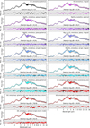 |
Fig. C.1 Best-fit spectra for all retrieval models listed in Table 6. From left to right, top to bottom, the ordering is identical to the model ordering of Table 6. The residuals of the winning model (SiO cloud with amorphous spherical particles in a two-column model with a global Fe cloud) are plotted in black below the respective residuals of all other models. |
Appendix D Best-fit opacities for all silicon-bearing species
In Fig. 2 we already showed the brightness temperature fits for the best 14 candidate silicate species. The fits for the remaining species considered in this work (see Table 2) are shown in Fig. D.1.
That is, TiO2 condensates are stable at higher temperatures than SiO.
All Tables
Ranked list of cloud opacity fits using the brightness temperature method for the wavelength range of 8–12.5 μm.
Properties of the parameter grids explored for the selfconsistent grid retrievals of the PSO J318 data.
All Figures
|
Fig. 1 Observations considered for the atmospheric characterization of PSO J318. Uppermost panel: all data considered for the spectral characterization of PSO J318at the wavelength binning fed into the retrieval and self-consistent grid model fits. Specifically, MIRI MRS data was binned down to λ/Δλ = 400, while NIRSpec G395H was binned to λ/Δλ = 400 and λ/Δλ = 1000 for NRS1 and NRS2, respectively. Second panel: HST WFC3, IRTF SpeX, and JWST NIRSpec PRISM data over the 1–3 μm wavelength range. Third panel: JWST NIRSpec G395H data at the full spectral resolution. Lowermost panel: JWST MIRI MRS data at the full spectral resolution. |
| In the text | |
|
Fig. 2 Opacity fits of the 10 μm feature for the “top 14” silicate cloud species using the brightness temperature method. The remaining fits for the less well fitting species can be found in Fig. D.1. |
| In the text | |
|
Fig. 3 Model fits of PSO J318 obtained with our fiducial two-column retrieval setup, considering different types of silicate clouds. Panel a shows the best-fit spectrum of the overall winning model (black solid line) plotted on top of the JWST data (gray circles, with 10b error scaling). The winning model assumes amorphous spherical SiO particles. The flux contribution of the two individual columns is also shown, at their best-fit relative scaling (salmon and rose colored lines, respectively). The light blue line shows the result of recalculating the best-fit model, but turning off the cloud opacities. Panel b shows the residuals between the best-fit model and the data (with 10b error scaling). Panel c is a version of Panel a that zooms in on the silicate feature, but the best-fit model is shown in pink instead. Panels d–m show the same zoomed-in view of the silicate feature but for the other tested silicate feature candidates. Panel n shows the residuals between model and data for the various silicate cloud species using the same colors as in panels c–m. |
| In the text | |
|
Fig. 4 Best-fit spectra and marginalized posterior distributions of the grid interpolation and free retrievals. First row: Exo-REM fit. Second row: ATMO fit. Third row: Sonora Diamondback fit. Fourth row: petitRADTRANS fit. Fifth row: Projected 1D posteriors for [M/H], C/O, 12C/13C, Teff, log10(g) and the radius R in the first to sixth column, respectively. For C/O, the posterior of the petitRADTRANS retrieval is shown twice because it was nominally calculated from the gas phase abundances only. For solar C/O, a ~ 25% reduction of gas phase oxygen is expected due to condensation (Sánchez-López et al. 2022), which we applied to the second, less opaque C/O posterior shown for petitRADTRANS. The last three rows show the posteriors obtained from considering the data’s 14 wavelength bands separately for the self-consistent grids, with the vertical dashed lines indicating the parameter grid values. |
| In the text | |
|
Fig. 5 Overview plot of the temperature, emission contribution, and cloud properties of the “winning” SiO cloud model with amorphous spherical particles, two atmospheric columns, and evolutionary priors. Panel a: retrieved pressure-temperature profiles. The pRT retrieval profile is shown in magenta. The 1–3 σ posterior regions of the temperature are indicated by progressively lighter magenta tones, but are difficult to distinguish because of the narrow posteriors. We also overplot the log10(g)-scaled P-T profiles of the grid models that are closest to the best-fit values obtained with species. Panel b: logarithmic emission contribution function of atmospheric Columns 1 and 2 as orange and purple contours. While nominally computed to sum to unity over all pressures at a given wavelength, the values have been scaled by the relative contribution of the two columns to the total atmospheric solution and multiplied by the wavelength-dependent flux. Panel c: size distribution of SiO cloud particles in Column 1 (shown in red), and Fe cloud particles in Column 1 and 2 (shown in blue and orange, respectively). For better comparability the distributions’ peak values have been normalized to the same y-axis values. The envelopes around the median distribution would correspond to the 1-σ uncertainty if the posterior variations around the median followed a Gauss distribution. Panel d: altitude-dependent cloud mass fraction of the SiO cloud (present in Column 1, shown in red) and of the Fe cloud (present in both Columns, shown in blue). The colored envelopes again represent the 1-σ uncertainty spread of the posterior distribution. The dashed lines correspond to the expected cloud deck position, obtained from intersecting the sampled P-T curves (see Panel a) with the saturation vapor pressure curves of SiO and Fe from Gail et al. (2013); Ackerman & Marley (2001). Panel e: SiO nucleation rate computed according to Gail et al. (2013). |
| In the text | |
|
Fig. 6 Evidence of 13CO absorption in PSO J318’s atmosphere. Left panel: best-fit spectrum of the winning pRT retrieval model (amorphous spherical SiO particles) post-processed to high spectral resolution (R = 3200, red solid line) and superimposed on the NIRSpec G395H NRS2 data of PSO J318 at full spectral resolution (black solid line). For comparison, pRT’s best-fit model for PSO J318 is also superimposed on a scaled version of VHS 1256b’s G395H spectrum from Miles et al. (2023) (blue solid line). Right panel: zoomed-in version of the left panel showing the data for PSO J318 as well as the pRT best-fit model, where in one case (cyan solid line) the 13CO opacity has been turned off in post-processing. |
| In the text | |
|
Fig. 7 Comparison between the 10μm flux of PSO J318 and the (scaled) flux of brown dwarfs and low-mass companions with mid-L and L-T transition spectral types. |
| In the text | |
|
Fig. C.1 Best-fit spectra for all retrieval models listed in Table 6. From left to right, top to bottom, the ordering is identical to the model ordering of Table 6. The residuals of the winning model (SiO cloud with amorphous spherical particles in a two-column model with a global Fe cloud) are plotted in black below the respective residuals of all other models. |
| In the text | |
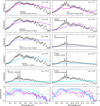 |
Fig. D.1 Similar to Fig. 2 but showing results for the remaining silicate species listed in Table 2. |
| In the text | |
Current usage metrics show cumulative count of Article Views (full-text article views including HTML views, PDF and ePub downloads, according to the available data) and Abstracts Views on Vision4Press platform.
Data correspond to usage on the plateform after 2015. The current usage metrics is available 48-96 hours after online publication and is updated daily on week days.
Initial download of the metrics may take a while.