| Issue |
A&A
Volume 703, November 2025
|
|
|---|---|---|
| Article Number | A300 | |
| Number of page(s) | 17 | |
| Section | Extragalactic astronomy | |
| DOI | https://doi.org/10.1051/0004-6361/202555890 | |
| Published online | 25 November 2025 | |
The effects of the environment on the central activity of galaxies as derived using mid-IR tracers
1
Centro de Astronomía (CITEVA), Universidad de Antofagasta, Avenida U. de Antofagasta, 02800 Antofagasta, Chile
2
Université Côte d’Azur, Observatoire de la Côte d’Azur, CNRS, Laboratoire Lagrange, 06000 Nice, France
3
Aix-Marseille Université, CNRS, LAM (Laboratoire d’Astrophysique de Marseille), UMR 7326, 13388 Marseille, France
4
Scientific associate INAF–Osservatorio Astronomico di Cagliari, Via della Scienza 5, 09047 Selargius, (CA), Italy
5
Leibniz-Institut für Astrophysik Potsdam (AIP), An der Sternwarte 16, 14482 Potsdam, Germany
⋆ Corresponding author: This email address is being protected from spambots. You need JavaScript enabled to view it.
Received:
10
June
2025
Accepted:
17
September
2025
Abstract
Aims. By exploiting photometry from the Wide-field Infrared Survey Explorer (WISE), we investigate the influence of environment and stellar mass on the prevalence of different excitation types in the interstellar gas of the central regions of galaxies in the Herschel Reference Survey (HRS, z ≈ 0.0047). We extend this analysis to a complementary sample of relatively nearby galaxies that are undergoing ram-pressure stripping (RPS, z ≈ 0.0195). Our goal is to assess whether a connection exists between active galactic nucleus (AGN) activity and either the cluster environment or the ram pressure stripping process.
Methods. We computed WISE mid-infrared colour indices from fluxes extracted from central apertures and applied two established mid-infrared diagnostic diagrams to distinguish AGN activity from non-AGN, and star-forming galaxy (SFG) excitation from that associated with ‘retired’ galaxies. The resulting types of excitation were then used in conjunction with stellar mass and environment classifications to construct a stellar mass-excitation fraction relation.
Results. The stellar mass-excitation fraction relation reveals that global stellar mass is the primary driver of excitation diversity in galaxy centres. In increasing order of prevalence, excitation types follow a sequence from SFGs to retired galaxies with increasing mass. The number of low-mass galaxies is too small to drive statistical tendencies. In contrast, SFG excitation becomes dominant at intermediate masses. At the highest mass end, the retired-galaxy type clearly prevails. Across the full mass range and in nearly all environments, SFG excitation is the most common, except for H I-gas deficient HRS galaxies, which are mostly retired. The excitation properties of galaxies undergoing RPS resemble those of HRS cluster members, field galaxies, and normal H I-content galaxies, minimising the environmental role. Contrary to previous results, we do not see any increase in AGN activity in H I-deficient cluster galaxies or in those undergoing RPS, since its fractions (∼10% for Seyfert 2 and ∼20% for low-ionisation nuclear emission-line region, LINER) remain largely unaffected along all environments.
Conclusions. These findings indicate that while rich environments are associated with certain excitation types, stellar mass remains the primary driver of excitation diversity in galaxy centres.
Key words: galaxies: active / galaxies: clusters: general / galaxies: evolution / galaxies: photometry
© The Authors 2025
 Open Access article, published by EDP Sciences, under the terms of the Creative Commons Attribution License (https://creativecommons.org/licenses/by/4.0), which permits unrestricted use, distribution, and reproduction in any medium, provided the original work is properly cited.
This article is published in open access under the Subscribe to Open model. This email address is being protected from spambots. You need JavaScript enabled to view it. to support open access publication.
1. Introduction
The evolution of galaxies is closely linked to the activity in their centres (e.g. Fabian 2012; Torres-Papaqui et al. 2013; López et al. 2023). In particular, quenching of star formation (SF) by active galactic nucleus (AGN) feedback (e.g. Fabian 2012; Yuma et al. 2013; George et al. 2019; Fluetsch et al. 2019; Radovich et al. 2019; Piotrowska et al. 2022) may trigger the transition to passive evolution (Faber et al. 2007).
Galactic centres mark the onset of stellar mass assembly through inside-out growth (e.g. Pérez et al. 2013; García-Benito et al. 2017; López Fernández et al. 2018). The physical process that gives rise to this cosmic evolution is SF, which concludes with the recognition of the star-forming galaxy (SFG) activity type. Star-forming galaxies (SFGs) are characterised by young stellar populations and blue regions hosting O-B type stars that strongly ionise the interstellar gas. Intense bursts of SF are usually observed, emitting strongly in the ultraviolet and infrared, the latter dominated by dust emission that reprocesses short-wavelength photons (Förster Schreiber & Wuyts 2020).
In contrast, AGN activity, whether secular or externally triggered, can change galaxy morphology and colour, fostering the development of a central bulge of old stars. At its core lies a non-thermal engine: an accreting supermassive black hole (SMBH), fed by the host galaxy gas that loses angular momentum. These engines can be powerful, dominating the host galaxy’s spectral features, especially in the X-ray and radio regimes (Netzer 2013, 2015; Ho 2008; Heckman & Best 2014).
More recently, a third phase has gained attention: ‘retired’1 activity, or rather inactivity. This phase corresponds to the final cosmic ages of stellar populations, and is associated with red, quiescent, gas-depleted galaxies, in which SF has ceased and SMBH fuelling has subsided. These galaxies exhibit weak optical line emission, are mostly dust-free, and their spectral energy distribution (SED) is dominated by hot, low-mass evolved stars and white dwarfs (Stasińska et al. 2008; Sarzi et al. 2010; Singh et al. 2013; Belfiore et al. 2015).
The classification of activity type is commonly based on the comparison of optical emission-line ratios and individual intensities (Baldwin et al. 1981; Veilleux & Osterbrock 1987; Lamareille et al. 2004; Lamareille 2010; Cid Fernandes et al. 2011), which trace the ionisation conditions of the interstellar gas. However, optical lines can be hard to detect due to instrumental sensitivity limitations and can also be weak because of dust attenuation, particularly at galaxy centres. Mid-infrared colour indices offer a robust alternative, capable of probing obscured regions effectively, as they are less affected by dust extinction since reprocessed radiation emits at these wavelengths (e.g. Mateos et al. 2012; Stern et al. 2012). For instance, WISE (Wide-field Infrared Survey Explorer, Wright et al. 2010) photometry, especially in its reddest passbands, remains reliable even at redshifts z ≳ 0.3 (see Caccianiga et al. 2015 and references therein).
In contrast, AGN hosts tend to be massive galaxies (e.g. Kauffmann et al. 2003, 2004; Fabian 2012; Pimbblet et al. 2013; Vitale et al. 2013; Lopes et al. 2017; Sánchez et al. 2018; Peluso et al. 2022), which more frequently show early-type morphologies (Baldry et al. 2004; Schawinski et al. 2007) and are commonly found in dense environments such as galaxy clusters (Dressler et al. 1997). This spatial clustering raises the question of whether AGN activity is environmentally driven. It has been widely accepted that galaxy clusters efficiently strip gas from galaxies, driving their rapid evolution (Boselli & Gavazzi 2006). One such phenomenon is ram pressure stripping (RPS; e.g. Gunn & Gott 1972; Vollmer et al. 2001; Kenney et al. 2004; Tonnesen et al. 2007; Ebeling et al. 2014; Boselli et al. 2016, 2022; Poggianti et al. 2016; Cramer et al. 2019), in which galaxies moving through the hot and dense intracluster medium experience a drag force that removes their interstellar gas. Recently, RPS has been proposed as a potential AGN trigger. For instance, Poggianti et al. (2017) report a high prevalence of AGN activity in jellyfish2 galaxies and suggest that ram pressure may funnel gas towards the SMBH, ultimately feeding AGN growth. Peluso et al. (2022) perform a follow-up analysis on a larger sample of jellyfish galaxies. However, the results of Poggianti et al. (2017) and Peluso et al. (2022) have recently been questioned by Boselli et al. (2022) and Cattorini et al. (2023), who find no observed increase in the AGN fraction in galaxies undergoing RPS. Indeed, the AGN fraction has been reported to be several times higher in field than in cluster galaxies (e.g. Dressler et al. 1985) and tends to decrease with increasing galaxy density (e.g. Kauffmann et al. 2004), although other studies suggest that the AGN fraction increases in dense, low-dispersion groups and that it may be similar in galaxy groups and clusters (e.g. Popesso & Biviano 2006; Shen et al. 2007).
To help clarify the ongoing debate around the potential connection between AGN activity and the dynamical interaction of galaxies with their surrounding medium, we explored the relation between stellar mass and gas-excitation processes across various environments. This analysis uses mid-infrared indicators focusing on central regions, where processes related to potential central engines are most likely to manifest, and probes obscured activity while minimising contamination from disc and halo components. Due to the WISE survey’s photometric resolution, we refer to ‘central’ rather than strictly ‘nuclear’ regions.
This paper is structured as follows. Section 2 describes the galaxy samples and data sources. Section 3 outlines the photometric procedures and mid-infrared diagnostic diagrams (mIRdds). In Section 4, we present the mIRdd classification scheme and analyse the excitation fractions as a function of environment through the stellar mass–excitation fraction relation. In Section 5, we compare our results with those obtained using alternative tracers, and in Section 6 we summarise our conclusions. In the appendices, we examine our reddest band fluxes, compare excitation classifications, and list the full photometric dataset.
2. Galaxy samples and data sources
2.1. The Herschel Reference Survey sample
This study is based on the Herschel Reference Survey (HRS; Boselli et al. 2010), a complete, volume-limited (D < 25 Mpc), K-band-selected sample of 323 nearby galaxies. The HRS spans a broad range of morphologies (excluding only under-represented blue compact and dwarf irregular galaxies), stellar masses, and environments–including the Virgo cluster and its surroundings.
The HRS galaxies were observed with the Herschel Space Telescope at 250, 350, and 500 μm. The K-band-flux selection ensures a well-defined stellar mass distribution and minimises dust-related biases, making the HRS a key reference for studies of dust and galaxy evolution.
In this analysis, we excluded 64 early-type galaxies (E and S0; Boselli et al. 2010), as RPS typically affects late-type galaxies infalling into clusters. The remaining late-type galaxies form the basis of the following environmental classification.
A significant fraction of HRS galaxies resides in the Virgo cluster. Following Gavazzi et al. (1999), Virgo cluster members (VCMs) are identified as galaxies belonging to the Virgo A and B subclusters, the North and East clouds, and the Southern Extension, and are included in the Virgo Cluster Catalogue (VCC ID, Binggeli et al. 1985).
Galaxies located outside the Virgo cluster but within nearby clouds–such as Leo, Ursa Major, the Ursa Major Southern Spur, Crater, Coma I, the Canes Venatici Spur, Canes Venatici-Camelopardalis, and Virgo-Libra (Boselli et al. 2010, their Fig. 1)–are here considered as ‘field’ galaxies.
Importantly, the distances for VCMs are fixed at 23 Mpc for galaxies in the Virgo B subcluster and 17 Mpc for the other members. For all remaining HRS galaxies, distances are based on recessional velocities, assuming  (Boselli et al. 2010).
To further assess potential external perturbations and gas depletion due to the Virgo intracluster medium, we used the H I deficiency parameters (DHI)3 from Boselli et al. (2014a), available for 315 HRS galaxies and calibrated following Boselli & Gavazzi (2009). Consistent with previous HRS works (e.g. Cortese et al. 2012a), galaxies with DHI ≥ 0.5 are considered H I-deficient, retaining < 32% of their expected H I mass.
2.2. The RPS galaxy sample
Galaxies with extended gas tails undergoing RPS have been observed in nearby clusters. In the Virgo, Leo, and Coma clusters, galaxies experiencing pure RPS are typically found at small virial radii, whereas RPS combined with other mechanisms tends to occur at larger radii (Boselli et al. 2022).
We identified 79 galaxies undergoing RPS by cross-matching the compilations of Boselli et al. (2022, their Table 2) and Tiwari et al. (2025, their Table 1). The cluster distribution is as follows: Virgo (24), Coma (A1656-38), Leo (A1367-11), Perseus (A426-4), and Norma (A3627-2). In Virgo, objects with detections of H I-gas tails account for ∼15%, possibly indicating modest RPS (Boselli et al. 2022). If RPS is taken solely as an indicator of process strength, about 59 galaxies in the sample are undergoing ‘strong’ RPS (see Table D.2). Consistent with expectations for infalling cluster populations, early-type galaxies are rare, with only 7/79 S0s (9%, none hosting an AGN; see Appendix D). These were excluded to ensure homogeneity between samples.
2.3. Data sources
2.3.1. The WISE survey
Surveying the mid-infrared sky, WISE achieved 5σ point-source sensitivities better than 0.08, 0.11, 1, and 6 mJy at four broad-wavelength bands centred at 3.4 (W1), 4.6 (W2), 11.6 (W3), and 22.1 μm (W4), respectively. Similarly, the angular resolution is 6.1, 6.4, 6.5, and 12.0 arcseconds (full width at half maximum). The astrometric precision for high signal-to-noise (S/N) sources is better than 0.15 arcseconds (Wright et al. 2010).
The Wide-field Infrared Survey Explorer (WISE) has provided an extensive infrared atlas, the legacy of which will endure for decades. For our study, we used photometric images from the WISE All-Sky Atlas Image Inventory Table at the Infrared Science Archive4.
2.3.2. Stellar masses
Stellar mass has been identified as the primary driver of galaxy evolution (e.g. Gavazzi & Scodeggio 1996; Boselli et al. 2001; Heavens et al. 2004; Asari et al. 2007; Ibarra-Medel et al. 2016; Catalán-Torrecilla et al. 2017). Consequently, stellar mass is used here as a reference for analysing different types of activity in galaxies.
Stellar masses of HRS galaxies were computed by Cortese et al. (2012b), following the prescription of Zibetti et al. (2009), using i-band luminosities and a g − i mass-to-light ratio. The masses of ten missing galaxies were taken from Boselli et al. (2015)–who use a relation between the H-band luminosity and a B-H mass-to-light ratio. All these masses were practically derived using a Chabrier (2003) initial mass function (IMF; see Table D.1). No stellar mass estimate was found for LCRSB123647.4−052325.
For the RPS sample, the stellar masses were mainly sourced from Boselli et al. (2022), consistently derived as in Cortese et al. (2012b). The masses for three cases computed by Boselli et al. (2022)–which might have been later rescaled to match their respective cluster distances–as well as those for galaxies in A426 calculated following Salim et al. (2007) using the Chabrier (2003) IMF–were retrieved from Tiwari et al. (2025) (see Table D.2).
Finally, Table 1 presents the distributions of stellar mass. Consistent with Cattorini et al. (2023), we divided the values into six bins (log M*, M⊙): M1 ≤ 8.5, 8.5 < M2 ≤ 9.0, 9.0 < M3 ≤ 9.5, 9.5 < M4 ≤ 10.0, 10.0 < M5 ≤ 10.5, and 10.5 < M6 (see Section 4.2).
Distributions of stellar mass (log M*, M⊙).
3. Methods
3.1. Photometric imaging processing
Our procedures consist of cleaning the images of unwanted sources, convolving them, converting counts to magnitudes or flux densities, and estimating and subtracting the background light.
3.1.1. Masking of unwanted objects
In this step, we discarded pixels corresponding to foreground stars and companion and background galaxies. We employed image segmentation from source detection in Python, using the detect_sources function from the photutils.segmentation package (Bradley et al. 2021). The function masked unwanted pixels by distinguishing them from those belonging to the object of interest. This distinction was based on a pixel-wise threshold, set at multiples of the image-data standard deviation of a sigma-clipped array. When stars were located in the foreground or when pixels from companion galaxies were too close, the threshold was continuously increased until such unwanted pixels were replaced with random background values.
3.1.2. Kernel convolution
Our convolution algorithm, used to bring all images to a common point spread function (PSF) and thus a common pixel resolution, is based on the method developed by Aniano et al. (2011). The high-resolution convolution kernel filters we used were also obtained from their repository5. Our algorithm adjusts the pixel scale of the kernel filters to match that of the original images and also normalises the former to ensure flux conservation.
As convolution must be performed towards broader PSFs, all images were matched to the W4 passband resolution, adopting a common FWHM of ∼12 arcsec. This standardisation imposes an inherent limitation, which is discussed in further detail in Section 3.1.4.
3.1.3. Computation of magnitudes and flux densities
For WISE data, DN refers to the source brightness measured in digital numbers. Vega-system magnitudes were computed using
 (1)
(1)
where MAGZP are the instrumental zero-point magnitudes: 20.5, 19.5, 18, and 13 mag for W1, W2, W3, and W4, respectively6. Flux densities (Fν, Jy) were computed from
 (2)
(2)
where Fν, zero are the zero-magnitude flux densities for Vega (Jarrett et al. 2011, their Table 1).
Importantly, since WISE images share a common field of view, no image reprojection or resampling to a common pixel grid was required. The reprojection is necessary when processing images from different surveys and photometric bands.
3.1.4. Background subtraction
Since no single background estimation method is universally applicable to a wide range of astronomical images, we determined the background and background noise levels using a two-step approach.
First, we selected several rectangular regions clearly outside the extensions of the galaxies and calculated their arithmetic means and standard deviations. From these, we respectively calculated a representative mean and standard deviation. The representative mean was subsequently subtracted from the image data. The resulting image serves as the input for the sep.extract() function–from the sep package for segmentation and analysis of astronomical images (Barbary 2016; Bertin & Arnouts 1996)–which uses the representative standard deviation to specify a pixel-by-pixel detection threshold. The statistical dispersion of object pixels increases compared to this threshold; thus, using increasing multiples of this limit allowed the detection of inner pixel regions of the objects. We then simulated concentric apertures to match the sizes of central regions and compared ‘integrated’ flux values–representatives of galaxy extensions–with those from reasonably defined ‘central’ apertures. We defined central regions to contain ≤ ∼ 5% of the pixels considered for representative main galaxy extensions (Tables D.1 and D.2). A standard detection threshold of 4.5 × σ was used for the integrated extensions or apertures.
Based on distances and optical diameters from Boselli et al. (2014a), central region diameters in the HRS range from ∼2.06 to 4.33 kpc, with a median of ∼3.12 kpc. At representative distances of 20 Mpc (HRS, z ≈ 0.0047) and 84 Mpc (RPS sample, z ≈ 0.0195), the W4 passband resolution (∼12 arcsec FWHM) corresponds to spatial scales of ∼1.2 and ∼4.9 kpc, respectively–comparable to our estimated central region sizes. At ∼1.2 kpc, WISE can distinguish broad features such as spiral arms and bulges, as in NGC4535 (HRS 204) or NGC4303 (HRS 114; see Fig. 1), but cannot resolve circumnuclear structures. This limitation is more pronounced at ∼4.9 kpc, where even the disc may be unresolved (e.g. ESO137-001, spatial resolution ∼4.1 kpc; see Fig. 1). Consequently, the W4 resolution is insufficient to isolate AGN emission–typically < 1 kpc in size (Netzer 2013)–from surrounding SF, making our use of central rather than nuclear apertures the most appropriate approach.
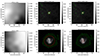 |
Fig. 1. Examples of background estimation in the W3 band: ESO137-001 (top) and NGC4303-HRS114 (bottom). From left to right, the background level and background-subtracted images are shown, illustrating the selected integrated and central apertures from object detection (red ellipses). Pixel value scales are shown on the right. The green contour levels correspond to 2, 3, 5, and 10 times the representative standard deviation, computed from the selected rectangular regions. |
Moreover, the sep.extract() function returns an array of the same dimensions as the original image, labelling pixels that clearly belong to the galaxy. Through visual inspection of the four-band output images, we find that galaxy extensions are roughly consistent across all bands. Therefore, we can use the labelled pixels from any band image to define the galaxy extension for the four images as flux variations are negligible.
In the second step, we used the Background2D() function from the photutils.background package (Bradley et al. 2021) for 2D background estimation, which involves the local calculation of the background and background RMS. The Background2D() function requires specifying the spatial size of the boxes in which the background is estimated. The background level within each box is computed as
 (3)
(3)
If (mean − median)/standard deviation > 0.3, the median is used instead. We masked pixels associated with the galaxy, as defined in the first step, as well as pixels with missing values.
This approach produces output images with a smooth variation in background levels across their extensions (see Fig. 1). Finally, in Appendix B, we test the reliability of our integrated W3 and W4 band fluxes.
3.2. The mid-infrared diagnostic diagrams (mIRdds)
To identify the dominant source of interstellar gas excitation in our galaxy samples, we used mid-infrared diagnostic diagrams (mIRdds) based on WISE photometry. These diagrams, which compare the colour indices W1−W2, W2−W3, and W3−W4, are sensitive to SF histories (SFHs), trace AGN activity and stellar populations (e.g. Jarrett et al. 2011, 2013; Coziol et al. 2014, 2015).
We used two mIRdds. The first (mIRdd I) compares W2−W3 versus W3−W4, distinguishing contributions from AGN and SF in the mid-infrared SEDs (see Coziol et al. 2014, 2015). The W2−W3 index traces warm dust heated by star-forming regions and is a strong indicator of SFG activity (e.g. Cluver et al. 2014; Herpich et al. 2016). Alone, W3 captures silicate absorption, Ne II, PAH, and AGN-related continuum emissions (Penny et al. 2015; Jarrett et al. 2011), while W4 reflects warm dust and reprocessed SF emission (Penny et al. 2015).
The second diagram (mIRdd II; e.g. Jarrett et al. 2011; Mateos et al. 2012; Caccianiga et al. 2015; Penny et al. 2015) compares W2−W3 with W1−W2, where AGNs, quasi-stellar objects (QSOs), and ultraluminous infrared galaxies (ULIRGs) occupy distinct regions (Jarrett et al. 2011). In particular, AGN-dominated systems can be identified using the Infrared Array Camera (IRAC) 1 and 2 passbands (|3.6|−|4.5| ≥ 0.5). Due to the close correspondence between IRAC 1-W1 and IRAC 2-W2 (WISE extractions with S/N > 5; see Jarrett et al. 2011), we consistently applied the W1−W2 ≥ 0.5 criterion (Stern et al. 2005; Jarrett et al. 2011). The W1−W2 ≥ 0.8 (Stern et al. 2012) represented a more stringent threshold, although exclusive to reliable X-ray AGN identifications.
Active galactic nuclei (AGNs) exhibit a characteristic red, power-law SED in the mid-infrared (fν ∝ να, with α ≤ −0.5; Alonso-Herrero et al. 2006). This signature, represented by a power-law curve in mIRdd II, is fully consistent with the AGN ‘wedge’ of Mateos et al. (2012).
Both mIRdds adopt the WHAN-based partition between SFG and emission-line-less (passive) galaxies, optimised for completeness and reliability (Cid Fernandes et al. 2011; Herpich et al. 2016). This partition also accounts for retired galaxies.
Finally, mIRdds such as these have been calibrated to identify AGN activity in local galaxies (z < 0.1; e.g. Cluver et al. 2020). Cluver et al. (2014, 2020) and Jarrett et al. (2023) use fixed apertures of 16.5 arcsec (∼5.5–8.2 kpc) to characterise total fluxes in nearby, compact systems. In contrast, we adopted smaller apertures tailored to the central regions, consistent with their physical scales (Section 3.1.4). Since Gavazzi et al. (2018) underline the importance of nuclear spectra for accurate AGN identification, our AGN counts (particularly of Sy2 classes, Section 4.1) show good agreement with theirs for the HRS sample (see Appendix C).
4. Analysis
4.1. Excitation classification using mIRdds
We constructed mIRdds for 257 HRS (including LCRSB123647.4052325) and 72 RPS galaxies using WISE colour indices derived from central aperture fluxes (Tables D.1 and D.2). To synthesise a classification scheme that incorporates information from both diagrams, Fig. 2 overlays the mIRdd I classifications–indicated by coloured geometric labels–onto mIRdd II.
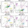 |
Fig. 2. Top: mIRdds for 257 late-type HRS galaxies (Boselli et al. 2010). Bottom: mIRdds for 72 late-type RPS galaxies (Boselli et al. 2022; Tiwari et al. 2025). All photometry is based on central apertures (median size ∼3.12 kpc for the HRS; see Section 3.1.4 and Appendix D). Left: mIRdd I (Coziol et al. 2014, 2015), with diagonal divisions separating AGN from SFG excitation, and between levels of SF (diagonal magenta and gold lines and bold labels, respectively). Excitation-type counts are listed at the bottom right. Right: mIRdd II (e.g. Jarrett et al. 2011; Mateos et al. 2012; Caccianiga et al. 2015; Herpich et al. 2016), featuring horizontal thresholds (dotted and dashed magenta lines and bold labels, aided by arrows) and the AGN wedge (magenta polygon) as defined by Stern et al. (2005, 2012), and Mateos et al. (2012). Coloured geometric labels for excitation types assigned in mIRdd I are consistently maintained in mIRdd II to ensure direct comparison and the derivation of a unified classification scheme across diagrams. Common features in both mIRdds as follows. The dashed brown line and bold labels mark the SFG-Retired galaxy divisor (Herpich et al. 2016). Dashed coloured contours represent 0.1 kernel density levels. The grey curve traces the model colour sequence for power-law spectra with annotated spectral indices (Wright et al. 2010, the K-dwarf star colour, K, is also plotted), illustrating the non-thermal radiation trend. Colours redden as the spectral index decreases, distinguishing galaxies (intrinsically redder) from stars (bluer). This sequence also reinforces the characteristic negative spectral indices of AGNs. |
For HRS galaxies (Fig. 2, top), mIRdd I reveals an important population of low-ionisation nuclear emission-line regions (LINERs; 0.44), followed by SFGs (0.38), Seyfert 2 (Sy2; 0.11) types, and a smaller, undefined ‘nd’ class (0.07) representing low-SF systems. Within their density contours in mIRdd I, Sy2 and LINER excitations follow a power-law sequence, fν ∝ να, with α ≈ −2 to 0.5 (grey curve). Notably, W2−W3 and W3−W4 colours decrease, causing roughly half of the LINER population to move towards the blue, suggesting their reclassification as retired galaxies (dashed brown line).
In contrast, mIRdd II generally agrees with the mIRdd I classification of SFGs but reclassifies red LINERs, nd, and Sy2 types as star-forming (dashed brown line), with only two cases exceeding the AGN thresholds (dotted and dashed magenta lines). Moreover, mIRdd II does not exhibit Sy2 and LINER types following the power-law sequence (grey curve), suggesting weaker AGN signatures. In mIRdd II indeed, the W2−W3 colour exhibits a more pronounced blueward variation than W1−W2, consistent with composite or low-luminosity AGNs, as also noted by Penny et al. (2015) and Jarrett et al. (2011).
The RPS mIRdd I (Fig. 2, bottom left) shows SFGs as the dominant population (0.54), followed by LINERs (0.32), Sy2 (0.13), and the nd types (0.01). Despite the smaller sample size, both Sy2 and LINER excitations in mIRdd I appear to follow the power-law curve, although some LINERs are dispersed towards the blue. The reclassification of red LINERs, nd, and Sy2 types as star-forming systems repeats in mIRdd II. In this case, however, five mIRdd I LINERs exceed the AGN thresholds, three of them likely being powerful AGNs (passing the dashed magenta line threshold). In other words, a significant fraction of LINERs in mIRdd I are reclassified as retired galaxies, yet some exhibit AGN emission in mIRdd II, suggesting a possible stronger AGN contribution than in the HRS sample (Fig. 2, right column, five at bottom versus one case at top).
Coziol et al. (2015) report that BL Lac objects occupy a similar region in mIRdd I as LINERs but exhibit slightly bluer W2−W3 colours. Their LINER sample is bluer by no more than W2−W3 = 1.5 mag, consistent with the threshold defined by Cluver et al. (2014). In this study, we adopt the more stringent SFG threshold proposed by Herpich et al. (2016), which allows us to better distinguish retired systems from LINERs (weak or low-luminosity AGNs; i.e. L[O III] λ5007 < 107 L⊙, Kauffmann et al. 2004) that may be misidentified in mIRdd I.
A synthesised classification framework should consider the diagnostic power of the W1−W2 index, based on the most sensitive WISE bands (Stern et al. 2012); the role of W3−W4 in distinguishing AGN from SFG excitation via dust emission (Coziol et al. 2015); and the overlap of W2−W3 indices between SFGs and both weak and strong (narrow-line Sy2 types; Kauffmann et al. 2004) AGNs (Jarrett et al. 2011; Penny et al. 2015). On this basis, we define four synthesised excitation classes (see Fig. 2) as follows:
-
SFG: mIRdd I SFGs with W1−W2 < 0.5 mag, and nd types with W2−W3 > 2.5 mag and W1−W2 < 0.5 mag.
-
Sy2: All types with W1−W2 ≥ 0.5 mag and W2−W3 > 2.5 mag, as well as Sy2s in mIRdd I.
-
LINER: LINERs and nd types with W1−W2 ≥ 0.5 mag and W2−W3 ≤ 2.5 mag, and LINERs with W2−W3 > 2.5 mag.
-
Retired: All remaining objects.
This classification provides the input for the stellar mass-excitation fraction analysis by environment (Section 4.2) and is compared with optical diagnostics in Appendix C.
4.2. The stellar mass-excitation fraction relation
Figure 3 and Table 2 present the relation between stellar mass and excitation fraction for the HRS and RPS samples. We begin with HRS field and H I-normal galaxies, which serve as reference populations for comparison with denser environments. We then examine VCMs and H I-deficient systems–likely affected by external perturbations–followed by a brief description of the RPS sample.
For galaxies in the field and with normal H I content, SFGs dominate the excitation fractions across all stellar masses, with values of 0.45 ± 0.06, and 0.55 ± 0.06, respectively. In contrast, LINER, retired, and Sy2 fractions remain consistently low, well below SFG levels, and within the random uncertainties (sqrt(N)). Along the stellar mass sequence, SFGs dominate at intermediate masses (M2–M5 bins), which are the most populated. LINER, Sy2, and retired fractions remain relatively constant across the mass bins, given the uncertainties. These trends should be interpreted with caution due to the limited sample sizes.
Alongside the above reference galaxies, VCMs and H I-deficient systems show the following. Across the full mass range, SFG fractions remain stable in VCMs, with values of 0.44 ± 0.06, but decline significantly in H I-deficient systems to 0.25 ± 0.05. This reduction is accompanied by an increase in retired excitation, which rises to 0.36 ± 0.07 in deficient galaxies while remaining unchanged in VCMs. The LINER and Sy2 fractions in VCMs remain low (0.24 ± 0.05 and 0.08 ± 0.03, respectively), similar, again, to field values. The same occurs for H I-deficient relative to normal systems, with Sy2 excitation (0.11 ± 0.04) being the only type showing clearly distinct fractions from the retired type. Along the mass sequence, the dominance of SFGs at intermediate masses is less pronounced in VCM galaxies, whereas retired excitation increases markedly among H I-deficient galaxies, especially at the highest masses. In the M5 mass bin, Sy2 fractions are comparable between VCM and field galaxies (within overlapping uncertainties), but a clear difference emerges between H I-deficient and normal systems, the latter showing no Sy2 excitation.
Although the RPS sample is the most statistically limited, it exhibits trends similar to those observed in field and H I-normal galaxies. There is no evidence for an increase in LINER and Sy2 excitation fractions, except for Sy2 in the M5 mass bin, which represents the highest Sy2 fraction overall but remains comparable to that of field galaxies within the uncertainties.
Table 2 supports the trends observed in Fig. 3, reinforcing that LINER and Sy2 excitations remain modest in the central regions of late-type galaxies and are insensitive to stellar mass and environment. Excitation associated with SFGs dominates in most cases, except in H I-deficient systems, where retired excitation becomes prevalent, suggesting that environment is secondary to stellar mass.
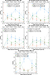 |
Fig. 3. Stellar mass-excitation fraction relation. Excitation types are based on mid-infrared colour diagnostics (mIRdds) representing central apertures (median size ∼3.12 kpc for the HRS). Section 2.1 details the HRS environmental classification. Stellar masses are binned from low to high (left to right): log (M*/M⊙), M1 ≤ 8.5, 8.5 < M2 ≤ 9.0, 9.0 < M3 ≤ 9.5, 9.5 < M4 ≤ 10.0, 10.0 < M5 ≤ 10.5, and 10.5 < M6. Top: Field and H I-normal galaxies. Middle: Virgo cluster members (VCMs) and H I-deficient galaxies. Bottom: Objects undergoing RPS in nearby clusters. Total galaxy counts are shown in the panel titles. Each panel lists excitation-type counts per mass bin (from left to right), with total counts and respective fractions shown on the rightmost side. The x axis labels indicate galaxy counts per stellar mass bin (top). Random uncertainties, indicated by vertical bars, are expressed as the ratio of the square root of each excitation-type count to the total. See also Tables 2, D.1, and D.2. |
4.2.1. AGNs in low-mass hosts and the trend with stellar mass
While AGN incidence typically increases with stellar mass (commonly found at log (M*/M⊙) ≳ 10), we detect a small number of Sy2 excitations in the low-mass (M1 and M2) bins of our field, H I-normal, and RPS samples (see Fig. 3). This raises the question of whether our mid-infrared diagnostics might misclassify AGNs at low stellar masses.
Low-mass, low-metallicity, intensely star-forming dwarf galaxies (W2−W3 > 4) can heat dust similarly to AGNs, producing WISE colours (W1−W2 > 0.5) that mimic AGN signatures and lead to misclassification (Hainline et al. 2016). Although we used W3−W4 to refine selection beyond the W1−W2 and W2−W3 criteria, we emphasise that AGN identification based on WISE colours in the low-mass regime requires extreme caution.
To test whether AGN activity is truly independent of stellar mass, we performed a bootstrap resampling of 100 stellar mass–matched subsets from field and H I-normal galaxies to match the mass distributions of the observed VCM, H I-deficient, and RPS samples. Median Sy2 fractions from these resampled subsets were compared to the fractions observed (see Fig. A.1). With the exception of the highest mass bin (M6), Sy2 fractions in VCM and H I-deficient galaxies align with results from Cattorini et al. (2023, WHAN-based) and remain distinct from the decreasing trend seen in field, H I-normal, and RPS galaxies–which might change if their few low-mass Sy2 detections are considered unreliable. However, overlapping uncertainties–especially for the RPS comparison–indicate no statistically significant enhancement in Sy2 incidence. While a mass-dependent increase in AGN activity is hinted at for VCM and H I-deficient galaxies, the limited sample sizes prevent robust conclusions regarding a mass dependence or environmental excess in Sy2 activity.
5. Discussion
Gravitational perturbations and hydrodynamic interactions are widely recognised as universal drivers of galaxy evolution in dense environments (Boselli et al. 2022 and references therein), and both are expected to influence AGN activity. In particular, galaxy-galaxy interactions are known to induce angular momentum loss that produces central gas inflows and thereby triggering AGN activity (e.g. Ellison et al. 2011, 2015, 2019). Similarly, galaxy mergers foster gas infall through instabilities, making them primary AGN triggering mechanisms across a range of redshifts (e.g. Gnedin 2003; Pimbblet et al. 2013; Marshall et al. 2018; Koulouridis & Bartalucci 2019).
Regarding hydrodynamic interactions, the role of RPS as an AGN trigger remains ambiguous. Although some simulations suggest that RPS can lead to angular momentum loss and central gas infall (Schulz & Struck 2001; Tonnesen & Bryan 2009; Ramos-Martínez et al. 2018), observational studies show that the stripped gas typically retains rotational motion near the disc (Fumagalli et al. 2014; Consolandi et al. 2017; Sardaneta et al. 2022), limiting its ability to feed an AGN. In certain edge-on interactions, modest or localised SF may instead be triggered at the interface between the stripped gas and the intracluster medium (Boselli et al. 2008, 2021; Nehlig et al. 2016; Lizée et al. 2021). Simulations suggest that such starburst episodes are short-lived, lasting only tens of Myr and not leading to enhanced AGN activity (Weinberg 2014; Troncoso-Iribarren et al. 2020).
Marshall et al. (2018) find that SF exceeds AGN activity across cluster-centric radii, with no significant increase in AGN incidence near cluster cores, a result consistent even at X-ray wavelengths (Koulouridis & Bartalucci 2019). Nevertheless, the connection between RPS and AGN activity remains under debate. Poggianti et al. (2017) report a high Sy2 fraction in a small sample of massive, late-type RPS galaxies, whereas Peluso et al. (2022) find a more moderate AGN excess (Sy2 + LINER) in similarly massive RPS systems. They estimate AGNs are 1.5 times more frequent in RPS galaxies compared to control systems; however, their result is derived from heterogeneous data and excludes low-mass and retired galaxies. Both studies rely on BPT diagnostics (Baldwin et al. 1981), which can misclassify retired systems as weak AGNs.
Conversely, using a larger sample, Kauffmann et al. (2004) report a decline in strong AGN fractions with increasing galaxy density, based on [O III] luminosity detections. Similarly, Roman-Oliveira et al. (2019), using the WHAN diagnostic (Cid Fernandes et al. 2010, 2011), detect AGNs in only five of 70 RPS-selected galaxies, with no phase-space correlation to regions of peak ram pressure (i.e. small cluster-centric radii with high differential velocities). Using a statistically significant local sample and standard optical emission-line diagnostics, Cattorini et al. (2023) find that Sy2 and LINER excitation fractions are largely independent of environment, with only LINERs showing a dependence on stellar mass, consistent with results from studies using the WHAN diagnostic. Their comparison of BPT and WHAN classifications highlights systematic differences in AGN classification, such that different schemes and the grouping of Sy2 types with LINERs may explain some of the above disparities. As noted by Boselli et al. (2022) and Cattorini et al. (2023), the predominant use of massive systems may overestimate AGN fractions. Lastly, Cattorini et al. (2023) show that AGN fractions can be nearly 60% higher when passive galaxies are excluded.
Our results in central regions of late-type galaxies show that Sy2 fractions remain consistently low compared to other excitation types and show invariance across environments and the stellar mass sequence. Fig. 3 and Table 2 suggest that neither cluster membership, RPS, nor stellar mass strongly influences AGN activity. Due to sample size limitations, particularly at the low-mass end that must be noted, we wonder whether our results can help to clarify this ongoing debate.
Table 3 reorganises the excitation-type fractions (see Table 2, ‘Total’ column) and further confirms the stability of Sy2 and LINER classifications across the five environments and the full stellar mass range. The Sy2 fractions range from 0.08 ± 0.03 in VCMs to 0.13 ± 0.03 and 0.14 ± 0.04 in field and RPS samples, with identical values between H I-normal and deficient galaxies. The LINER fractions range from 0.22 ± 0.04 (H I-normal) to 0.28 ± 0.06 (deficient), with minimal variation across environments (including the RPS sample, 0.19 ± 0.05). The SFG and retired excitations are similarly stable among VCM, field, and RPS galaxies but vary significantly between H I-normal and deficient systems. Hence, in the central regions of late-type galaxies, the excitation frequencies–particularly those related to AGN–are largely unaffected in cluster, RPS, and field galaxies, whereas retired and SFG excitations vary more strongly with neutral gas mass.
Across RPS, field, and H I-normal galaxies, excitation fractions are remarkably consistent, with SFG dominating in all environments except H I-deficient systems, where neutral gas depletion limits SF. These gas-poor galaxies are typically located in clusters, with deficiency increasing towards the cluster core, where RPS is most effective (Warmels 1986; Cayatte et al. 1990, 1994; Bravo-Alfaro et al. 2000; Chung et al. 2009; Loni et al. 2021). In such systems, the gaseous disc is truncated relative to the stellar disc, indicating outside-in stripping (Boselli & Gavazzi 2006; Boselli et al. 2022, and references therein). The removal of gas quenches SF (Boselli et al. 2014b) leading to the truncation of young stellar populations, as traced by recombination line emission (e.g. Koopmann et al. 2006; Boselli & Gavazzi 2006; Cortese et al. 2012b; Fossati et al. 2013).
The H I-normal galaxies exhibit no Sy2 detections in the 10.0 < log (M*/M⊙) ≤ 10.5 (M5) range. This absence, contrasting with detections in H I-deficient and RPS galaxies, suggests a potential environmental influence on AGN incidence. Only studies with significantly larger samples can determine whether this absence is real or a result of sample incompleteness.
Although LINERs are identified under a strict SF threshold (Section 4.1), low-ionisation emission from evolved stars may still be significant (e.g. Belfiore et al. 2015, 2016, 2017). An increase in such ‘fake’ AGNs is plausible in cluster environments where gas removal quenches central SF, leaving old stellar populations as the dominant ionising source–particularly in low-mass systems that lack enough gravitational potential to retain their central gas (unlike NGC4569, Boselli et al. 2006). Based on our synthesised classification, we find no increase in LINER fractions from low- to high-density environments, although our small sample sizes warrant cautious interpretation.
Hydrodynamical simulations by Ricarte et al. (2020), capable of producing tails in infalling systems, indicate that black hole accretion can increase during pericentric passages of gas-rich massive galaxies, but this effect depends on the ability of the galaxy to retain cold gas. Enhancement of AGN activity is therefore more likely at higher redshifts, where galaxies are more gas-rich. This is consistent with observations reporting increasing AGN fractions in clusters at increasing redshifts (e.g. Martini et al. 2013; Bufanda et al. 2017). In contrast, AGN incidence may remain low in gas-poor systems within dynamically relaxed, nearby clusters.
From an X-ray perspective, Tiwari et al. (2025) find no significant difference in central point source luminosities between 29 RPS and 40 control galaxies, suggesting that any RPS-driven AGN activity is weak or transient. When moderate-to-low-luminosity X-ray point sources are considered, AGN fractions remain broadly constant with galaxy density, further supporting the environmental independence of AGN activity (Tiwari et al. 2025, and references therein).
In this work, we employed a synthesised mid-infrared excitation classification method, which to the best of our knowledge, has not been applied previously in this context. Despite sample size limitations, our findings are consistent with optical (Gavazzi et al. 2018; Roman-Oliveira et al. 2019; Cattorini et al. 2023) and X-ray (Tiwari et al. 2025) results, reinforcing the need for multi-wavelength approaches to AGN identification. Our results suggest that the choice of classification scheme may be less critical than ensuring stellar mass completeness and inclusion of passive systems. Radio-based AGN classification could offer valuable complementary constraints in future work.
6. Summary and conclusions
To explore the potential link between AGN activity and cluster environment or RPS, we have analysed gas excitation fractions as a function of stellar mass and environment in central regions of galaxies from the HRS (Boselli et al. 2010) and a sample of objects undergoing RPS (Boselli et al. 2022; Tiwari et al. 2025). We focused on late-type systems, typically affected by RPS. Two mid-infrared diagnostic diagrams–based on colours computed from the WISE All-Sky Atlas Image Inventory Table–were used to classify strong and weak AGN-like activity (Sy2 and LINER), ongoing SF, and retired excitation (Section 3.2).
Using the excitation types (Section 4.1), environmental classifications (Section 2.1), and stellar masses (log (M*/M⊙), ∼7.39–11.34; Section 2.3.2), we constructed the stellar mass-excitation fraction relation for HRS galaxies (divided into Virgo cluster members (VCM), field, H I-deficient and H I-normal), and the RPS sample (see Fig. 3, and Tables 2 and 3). Our main results are as follows.
Along the stellar mass sequence:
-
Sy2 and LINER excitations remain consistently low and largely invariant across VCM, field, H I-deficient and H I-normal, and RPS environments. At intermediate most frequent masses, star-forming galaxies (SFGs) dominate all excitation classifications, with consistent fractions in nearly all environments. Retired excitation prevails at the high-mass end in all environments (except H I-normal) and also along the mass sequence for H I-deficient–breaking the general SFG→retired progression as mass increases, and representing the only case where environment overcomes stellar mass.
-
RPS galaxies follow trends similar to those of VCM, field and H I-normal systems, with no clear enhancement in Sy2 and LINER types.
-
These results confirm that the AGN (Sy2) and LINER classifications are fairly constant in the central regions of late-type galaxies and do not show any clear increase in cluster, H I-deficient, or RPS galaxies. In contrast, variations in SFG and retired excitation are more closely linked to the neutral-gas content.
Across the full mass range:
-
Sy2 fractions range from 0.08 ± 0.03 to 0.14 ± 0.04, while LINER fractions range from 0.19 ± 0.05 to 0.28 ± 0.06, showing no significant environmental dependence. This agrees with studies of the AGN-RPS connection in the optical and X-ray regimes, both in low- and high-density environments, although some other studies report the opposite trend.
In conclusion, SFG excitation is the most common in central regions, consistently exceeding the combined Sy2 (AGN) and LINER fractions in all environments except H I-deficient galaxies–where environmental influence is most evident. There is a trend of increasing AGN fraction with stellar mass in VCM and H I-deficient galaxies, although the overall results are limited by the small number of cases and caution is needed when interpreting AGN activity at low masses (log (M*/M⊙) < 9.5). Strong (Sy2) and weak (LINER) AGN fractions remain invariant, indicating independence from environment. In contrast, SFG and retired excitations show sensitivity to neutral gas content. Overall, in the central regions of late-type HRS and RPS galaxies, the excitations that fluctuate significantly are neither Sy2 nor LINER.
Data availability
Tables D.1 and D.2 are available at the CDS via https://cdsarc.cds.unistra.fr/viz-bin/cat/J/A+A/703/A300
Acknowledgments
We thank the anonymous referee for valuable comments that improved this study. M. Boquien acknowledges support from the ANID BASAL project FB210003. This study was supported by the French government through the France 2030 investment plan managed by the National Research Agency (ANR), as part of the initiative of Excellence of Université Côte d’Azur under reference number ANR-15-IDEX-01. C. Nitschelm and A. Morales-Vargas acknowledge the funding provided by the ASTRO20-0039 ANID project. O. Dorey was supported by the ANID BASAL project FB210003, as well as the Programa de Doctorado en Astrofísica y Astroinformática of the Universidad de Antofagasta. This work presents redshifts and other information from the NASA Extragalactic Database (NED) (https://ned.ipac.caltech.edu/). Data management and figures for this paper were possible by the use of R (https://www.r-project.org/): A language and environment for statistical computing. R Foundation for Statistical Computing, Vienna, Austria. Raquel, Alberto e Isaías: Mateo y yo les dedicamos este modesto trabajo... es para ustedes.
References
- Alonso-Herrero, A., Perez-Gonzalez, P. G., Alexander, D. M., et al. 2006, ApJ, 640, 167 [Google Scholar]
- Aniano, G., Draine, B. T., Gordon, K. D., & Sandstrom, K. 2011, PASP, 123, 1218 [Google Scholar]
- Asari, N. V., Cid Fernandes, R., Stasińska, G., et al. 2007, MNRAS, 381, 263 [Google Scholar]
- Baldry, I. K., Glazebrook, K., Brinkmann, J., et al. 2004, ApJ, 600, 681 [Google Scholar]
- Baldwin, J. A., Phillips, M. M., & Terlevich, R. 1981, PASP, 93, 5 [Google Scholar]
- Barbary, K. 2016, J. Open Source Software, 1, 58 [NASA ADS] [CrossRef] [Google Scholar]
- Belfiore, F., Maiolino, R., Bundy, K., et al. 2015, MNRAS, 449, 867 [NASA ADS] [CrossRef] [Google Scholar]
- Belfiore, F., Maiolino, R., Maraston, C., et al. 2016, MNRAS, 461, 3111 [Google Scholar]
- Belfiore, F., Maiolino, R., Maraston, C., et al. 2017, MNRAS, 466, 2570 [Google Scholar]
- Bertin, E., & Arnouts, S. 1996, A&AS, 117, 393 [NASA ADS] [CrossRef] [EDP Sciences] [Google Scholar]
- Binggeli, B., Sandage, A., & Tammann, G. A. 1985, AJ, 90, 1681 [Google Scholar]
- Boselli, A., & Gavazzi, G. 2006, PASP, 118, 517 [Google Scholar]
- Boselli, A., & Gavazzi, G. 2009, A&A, 508, 201 [NASA ADS] [CrossRef] [EDP Sciences] [Google Scholar]
- Boselli, A., Gavazzi, G., Donas, J., & Scodeggio, M. 2001, AJ, 121, 753 [NASA ADS] [CrossRef] [Google Scholar]
- Boselli, A., Boissier, S., Cortese, L., et al. 2006, ApJ, 651, 811 [Google Scholar]
- Boselli, A., Boissier, S., Cortese, L., & Gavazzi, G. 2008, ApJ, 674, 742 [Google Scholar]
- Boselli, A., Eales, S., Cortese, L., et al. 2010, PASP, 122, 261 [Google Scholar]
- Boselli, A., Cortese, L., & Boquien, M. 2014a, A&A, 564, A65 [NASA ADS] [CrossRef] [EDP Sciences] [Google Scholar]
- Boselli, A., Voyer, E., Boissier, S., et al. 2014b, A&A, 570, A69 [NASA ADS] [CrossRef] [EDP Sciences] [Google Scholar]
- Boselli, A., Fossati, M., Gavazzi, G., et al. 2015, A&A, 579, A102 [NASA ADS] [CrossRef] [EDP Sciences] [Google Scholar]
- Boselli, A., Cuillandre, J. C., Fossati, M., et al. 2016, A&A, 587, A68 [NASA ADS] [CrossRef] [EDP Sciences] [Google Scholar]
- Boselli, A., Lupi, A., Epinat, B., et al. 2021, A&A, 646, A139 [NASA ADS] [CrossRef] [EDP Sciences] [Google Scholar]
- Boselli, A., Fossati, M., & Sun, M. 2022, A&ARv, 30, 3 [NASA ADS] [CrossRef] [Google Scholar]
- Bradley, L., Sipőcz, B., Robitaille, T., et al. 2021, https://doi.org/10.5281/zenodo.4624996 [Google Scholar]
- Bravo-Alfaro, H., Cayatte, V., van Gorkom, J. H., & Balkowski, C. 2000, AJ, 119, 580 [Google Scholar]
- Bufanda, E., Hollowood, D., Jeltema, T. E., et al. 2017, MNRAS, 465, 2531 [NASA ADS] [CrossRef] [Google Scholar]
- Caccianiga, A., Antón, S., Ballo, L., et al. 2015, MNRAS, 451, 1795 [NASA ADS] [CrossRef] [Google Scholar]
- Catalán-Torrecilla, C., Gil de Paz, A., Castillo-Morales, A., et al. 2017, ApJ, 848, 87 [Google Scholar]
- Cattorini, F., Gavazzi, G., Boselli, A., & Fossati, M. 2023, A&A, 671, A118 [NASA ADS] [CrossRef] [EDP Sciences] [Google Scholar]
- Cayatte, V., van Gorkom, J. H., Balkowski, C., & Kotanyi, C. 1990, AJ, 100, 604 [NASA ADS] [CrossRef] [Google Scholar]
- Cayatte, V., Kotanyi, C., Balkowski, C., & van Gorkom, J. H. 1994, AJ, 107, 1003 [Google Scholar]
- Chabrier, G. 2003, PASP, 115, 763 [Google Scholar]
- Chung, A., van Gorkom, J. H., Kenney, J. D. P., Crowl, H., & Vollmer, B. 2009, AJ, 138, 1741 [Google Scholar]
- Cid Fernandes, R., Stasińska, G., & Schlickmann, M. S. 2010, MNRAS, 403, 1036 [NASA ADS] [CrossRef] [Google Scholar]
- Cid Fernandes, R., Stasińska, G., Mateus, A., & Asari, N. V. 2011, MNRAS, 413, 1687 [NASA ADS] [CrossRef] [Google Scholar]
- Ciesla, L., Boquien, M., Boselli, A., et al. 2014, A&A, 565, A128 [NASA ADS] [CrossRef] [EDP Sciences] [Google Scholar]
- Cluver, M. E., Jarrett, T. H., Hopkins, A. M., et al. 2014, ApJ, 782, 90 [Google Scholar]
- Cluver, M. E., Jarrett, T. H., Taylor, E. N., et al. 2020, ApJ, 898, 20 [NASA ADS] [CrossRef] [Google Scholar]
- Consolandi, G., Gavazzi, G., Fossati, M., et al. 2017, A&A, 606, A83 [NASA ADS] [CrossRef] [EDP Sciences] [Google Scholar]
- Cortese, L., Ciesla, L., Boselli, A., et al. 2012a, A&A, 540, A52 [NASA ADS] [CrossRef] [EDP Sciences] [Google Scholar]
- Cortese, L., Boissier, S., Boselli, A., et al. 2012b, A&A, 544, A101 [NASA ADS] [CrossRef] [EDP Sciences] [Google Scholar]
- Coziol, R., Torres-Papaqui, J. P., Plauchu-Frayn, I., et al. 2014, RMxAA, 50, 255 [Google Scholar]
- Coziol, R., Torres-Papaqui, J. P., & Andernach, H. 2015, AJ, 149, 192 [Google Scholar]
- Cramer, W. J., Kenney, J. D. P., Sun, M., et al. 2019, ApJ, 870, 63 [Google Scholar]
- Dressler, A., Thompson, I. B., & Shectman, S. A. 1985, ApJ, 288, 481 [NASA ADS] [CrossRef] [Google Scholar]
- Dressler, A., Oemler, A., Jr., Couch, W. J., et al. 1997, ApJ, 490, 577 [NASA ADS] [CrossRef] [Google Scholar]
- Ebeling, H., Stephenson, L. N., & Edge, A. C. 2014, ApJ, 781, L40 [Google Scholar]
- Ellison, S. L., Patton, D. R., Mendel, J. T., & Scudder, J. M. 2011, MNRAS, 418, 2043 [NASA ADS] [CrossRef] [Google Scholar]
- Ellison, S. L., Patton, D. R., & Hickox, R. C. 2015, MNRAS, 451, L35 [NASA ADS] [CrossRef] [Google Scholar]
- Ellison, S. L., Viswanathan, A., Patton, D. R., et al. 2019, MNRAS, 487, 2491 [NASA ADS] [CrossRef] [Google Scholar]
- Faber, S. M., Willmer, C. N. A., Wolf, C., et al. 2007, ApJ, 665, 265 [Google Scholar]
- Fabian, A. C. 2012, ARA&A, 50, 455 [Google Scholar]
- Fluetsch, A., Maiolino, R., Carniani, S., et al. 2019, MNRAS, 483, 4586 [NASA ADS] [Google Scholar]
- Förster Schreiber, N. M., & Wuyts, S. 2020, ARA&A, 58, 661 [Google Scholar]
- Fossati, M., Gavazzi, G., Savorgnan, G., et al. 2013, A&A, 553, A91 [NASA ADS] [CrossRef] [EDP Sciences] [Google Scholar]
- Fumagalli, M., Fossati, M., & Hau, G. K. T. 2014, MNRAS, 445, 4335 [Google Scholar]
- García-Benito, R., González Delgado, R. M., Pérez, E., et al. 2017, A&A, 608, A27 [NASA ADS] [CrossRef] [EDP Sciences] [Google Scholar]
- Gavazzi, G., & Scodeggio, M. 1996, A&A, 312, L29 [NASA ADS] [Google Scholar]
- Gavazzi, G., Boselli, A., Scodeggio, M., Pierini, D., & Belsole, E. 1999, MNRAS, 304, 595 [Google Scholar]
- Gavazzi, G., Savorgnan, G., & Fumagalli, M. 2011, A&A, 534, A31 [NASA ADS] [CrossRef] [EDP Sciences] [Google Scholar]
- Gavazzi, G., Consolandi, G., Belladitta, S., Boselli, A., & Fossati, M. 2018, A&A, 615, A104 [NASA ADS] [CrossRef] [EDP Sciences] [Google Scholar]
- George, K., et al. 2019, MNRAS, 487, 3102 [Google Scholar]
- Gnedin, O. Y. 2003, ApJ, 582, 141 [Google Scholar]
- Gunn, J. E., & Gott, J. R., III. 1972, ApJ, 176, 1 [NASA ADS] [CrossRef] [Google Scholar]
- Hainline, K. N., Reines, A. E., Greene, J. E., & Stern, D. 2016, ApJ, 832, 119 [CrossRef] [Google Scholar]
- Haynes, M., & Giovanelli, R. 1984, AJ, 89, 758 [NASA ADS] [CrossRef] [Google Scholar]
- Heavens, A., Panter, B., Jimenez, R., & Dunlop, J. 2004, Nature, 428, 625 [CrossRef] [Google Scholar]
- Heckman, T. M., & Best, P. N. 2014, ARA&A, 52, 589 [Google Scholar]
- Herpich, F., Mateus, A., Stasińska, G., Cid Fernandes, R., & Asari, N. V. 2016, MNRAS, 462, 1826 [NASA ADS] [CrossRef] [Google Scholar]
- Ho, L. C. 2008, ARA&A, 46, 475 [Google Scholar]
- Ibarra-Medel, H. J., Sánchez, S. F., Avila-Reese, V., et al. 2016, MNRAS, 463, 2799 [NASA ADS] [CrossRef] [Google Scholar]
- Jarrett, T. H., Cohen, M., Masci, F., et al. 2011, ApJ, 735, 112 [Google Scholar]
- Jarrett, T. H., Masci, F., Tsai, C. W., et al. 2013, AJ, 145, 6 [Google Scholar]
- Jarrett, T. H., Cluver, M. E., Taylor, E. N., et al. 2023, ApJ, 946, 95 [NASA ADS] [CrossRef] [Google Scholar]
- Kauffmann, G., Heckman, T. M., Tremonti, C., et al. 2003, MNRAS, 346, 1055 [Google Scholar]
- Kauffmann, G., White, S. D. M., Heckman, T. M., et al. 2004, MNRAS, 353, 713 [Google Scholar]
- Kenney, J. D. P., van Gorkom, J. H., & Vollmer, B. 2004, AJ, 127, 3361 [Google Scholar]
- Koopmann, R. A., Haynes, M. P., & Catinella, B. 2006, AJ, 131, 716 [NASA ADS] [CrossRef] [Google Scholar]
- Koulouridis, E., & Bartalucci, I. 2019, A&A, 623, L10 [EDP Sciences] [Google Scholar]
- Lamareille, F. 2010, A&A, 509, A53 [CrossRef] [EDP Sciences] [Google Scholar]
- Lamareille, F., Mouhcine, M., Contini, T., Lewis, I., & Maddox, S. 2004, MNRAS, 350, 396 [NASA ADS] [CrossRef] [Google Scholar]
- Lizée, T., Vollmer, B., Braine, J., & Nehlig, F. 2021, A&A, 645, A111 [NASA ADS] [CrossRef] [EDP Sciences] [Google Scholar]
- Loni, A., Serra, P., Kleiner, D., et al. 2021, A&A, 648, A31 [NASA ADS] [CrossRef] [EDP Sciences] [Google Scholar]
- Lopes, P. A. A., Ribeiro, A. L. B., & Rembold, S. B. 2017, MNRAS, 472, 409 [NASA ADS] [CrossRef] [Google Scholar]
- López Fernández, R., González Delgado, R. M., Pérez, E., et al. 2018, A&A, 615, A27 [NASA ADS] [CrossRef] [EDP Sciences] [Google Scholar]
- López, I. E., Brusa, M., Bonoli, S., et al. 2023, A&A, 672, A137 [NASA ADS] [CrossRef] [EDP Sciences] [Google Scholar]
- Marshall, M. A., Shabala, S. S., Krause, M. G. H., et al. 2018, MNRAS, 474, 3615 [NASA ADS] [CrossRef] [Google Scholar]
- Martini, P., Miller, E. D., Brodwin, M., et al. 2013, ApJ, 768, 1 [Google Scholar]
- Mateos, S., Alonso-Herrero, A., Carrera, F. J., et al. 2012, MNRAS, 426, 3271 [Google Scholar]
- Nehlig, F., Vollmer, B., & Braine, J. 2016, A&A, 587, A108 [NASA ADS] [CrossRef] [EDP Sciences] [Google Scholar]
- Netzer, H. 2013, The Physics and Evolution of Active Galactic Nuclei (Cambridge University Press) [Google Scholar]
- Netzer, H. 2015, ARA&A, 53, 365 [Google Scholar]
- Peluso, G., Vulcani, B., Poggianti, B. M., et al. 2022, ApJ, 927, 130 [NASA ADS] [CrossRef] [Google Scholar]
- Penny, S. J., Brown, M. J. I., Pimbblet, K. A., et al. 2015, MNRAS, 453, 3519 [Google Scholar]
- Pérez, E., Cid Fernandes, R., González Delgado, R. M., et al. 2013, ApJ, 764, L1 [Google Scholar]
- Pimbblet, K. A., Shabala, S. S., Haines, C. P., Fraser-McKelvie, A., & Floyd, D. J. E. 2013, MNRAS, 429, 1827 [NASA ADS] [CrossRef] [Google Scholar]
- Piotrowska, J. M., Bluck, A. F. L., Maiolino, R., & Peng, Y. 2022, MNRAS, 512, 1052 [NASA ADS] [CrossRef] [Google Scholar]
- Poggianti, B. M., Fasano, G., Omizzolo, A., et al. 2016, AJ, 151, 78 [Google Scholar]
- Poggianti, B. M., Jaffé, Y. L., Moretti, A., et al. 2017, Nature, 548, 304 [Google Scholar]
- Popesso, P., & Biviano, A. 2006, A&A, 460, L23 [NASA ADS] [CrossRef] [EDP Sciences] [Google Scholar]
- Radovich, M., Poggianti, B., Jaffé, Y. L., et al. 2019, MNRAS, 486, 486 [Google Scholar]
- Ramos-Martínez, M., Gómez, G. C., & Pérez-Villegas, A. 2018, MNRAS, 476, 3781 [CrossRef] [Google Scholar]
- Ricarte, A., Tremmel, M., Natarajan, P., & Quinn, T. 2020, ApJ, 895, L8 [NASA ADS] [CrossRef] [Google Scholar]
- Roman-Oliveira, F. V., Chies-Santos, A. L., Rodríguez del Pino, B., et al. 2019, MNRAS, 484, 892 [Google Scholar]
- Salim, S., Rich, R. M., Charlot, S., et al. 2007, ApJS, 173, 267 [NASA ADS] [CrossRef] [Google Scholar]
- Sánchez, S. F., Avila-Reese, V., Hernandez-Toledo, H., et al. 2018, RMxAA, 54, 217 [Google Scholar]
- Sardaneta, M. M., Amram, P., Boselli, A., et al. 2022, A&A, 659, A45 [NASA ADS] [CrossRef] [EDP Sciences] [Google Scholar]
- Sarzi, M., Shields, J. C., Schawinski, K., et al. 2010, MNRAS, 402, 2187 [Google Scholar]
- Schawinski, K., Thomas, D., Sarzi, M., et al. 2007, MNRAS, 382, 1415 [Google Scholar]
- Schulz, S., & Struck, C. 2001, MNRAS, 328, 185 [NASA ADS] [CrossRef] [Google Scholar]
- Shen, Y., Mulchaey, J. S., Raychaudhury, S., Rasmussen, J., & Ponman, T. J. 2007, ApJ, 654, L115 [Google Scholar]
- Singh, R., van de Ven, G., Jahnke, K., et al. 2013, A&A, 558, A43 [NASA ADS] [CrossRef] [EDP Sciences] [Google Scholar]
- Stasińska, G., Vale Asari, N., Cid Fernandes, R., et al. 2008, MNRAS, 391, L29 [NASA ADS] [Google Scholar]
- Stern, D., Eisenhardt, P., Gorjian, V., et al. 2005, ApJ, 631, 163 [Google Scholar]
- Stern, D., Assef, R. J., Benford, D. J., et al. 2012, ApJ, 753, 30 [Google Scholar]
- Tiwari, J., Sun, M., Luo, R., et al. 2025, ApJ, 979, 134 [Google Scholar]
- Tonnesen, S., & Bryan, G. L. 2009, ApJ, 694, 789 [NASA ADS] [CrossRef] [Google Scholar]
- Tonnesen, S., Bryan, G. L., & van Gorkom, J. H. 2007, ApJ, 671, 1434 [Google Scholar]
- Torres-Papaqui, J. P., Coziol, R., Plauchu-Frayn, I., et al. 2013, RMxAA, 49, 311 [Google Scholar]
- Troncoso-Iribarren, P., Padilla, N., Santander, C., et al. 2020, MNRAS, 497, 4145 [Google Scholar]
- Veilleux, S., & Osterbrock, D. E. 1987, ApJS, 63, 295 [Google Scholar]
- Vitale, M., Mignoli, M., Cimatti, A., et al. 2013, A&A, 556, A11 [NASA ADS] [CrossRef] [EDP Sciences] [Google Scholar]
- Vollmer, B., Cayatte, V., Balkowski, C., & Duschl, W. J. 2001, ApJ, 561, 708 [NASA ADS] [CrossRef] [Google Scholar]
- Warmels, R. H. 1986, HI Properties of Spiral Galaxies in the Virgo Cluster PhDT 105 [Google Scholar]
- Weinberg, M. D. 2014, MNRAS, 438, 3007 [Google Scholar]
- Wright, E. L., Eisenhardt, P. R. M., Mainzer, A. K., et al. 2010, AJ, 140, 1868 [Google Scholar]
- Yuma, S., Ouchi, M., Drake, A. B., et al. 2013, ApJ, 779, 53 [NASA ADS] [CrossRef] [Google Scholar]
- Zibetti, S., Charlot, S., & Rix, H.-W. 2009, MNRAS, 400, 1181 [NASA ADS] [CrossRef] [Google Scholar]
Retired and so-called ‘passive’ galaxies share similar stellar populations and have not formed stars in the past 100 Myr (Cid Fernandes et al. 2011). Thus, both are considered retired and evolving passively. However, passive galaxies lack emission lines (Herpich et al. 2016).
Galaxies undergoing severe RPS develop tentacle-like structures that extend beyond their discs, stretching several kiloparsecs in length.
The DHI parameter is defined as the logarithmic difference between the expected H I mass–assuming the galaxy were in isolation–and the observed H I mass for a galaxy of a given angular size and morphology (Haynes & Giovanelli 1984).
Photometric calibration: https://wise2.ipac.caltech.edu/docs/release/prelim/expsup
Corrections for underlying absorption are primarily applied to bright galaxies, which are often bulge-dominated.
As previously noted, LCRSB123647.4-052325 is a special case and the only galaxy excluded from the respective analysis.
Appendix A: Resampling for the stellar mass trend
To explore the apparent insensitivity of AGN activity to stellar mass reported in Section 4.2, we performed a bootstrap resampling by extracting 100 subsets that reproduce the stellar mass distributions of VCM, H I-deficient, and RPS galaxies, using their field and H I-normal counterparts as parent populations. From these mass-matched subsets, we computed the median Sy2 fractions, comparing them to the original fractions observed in the VCM, H I-deficient, and RPS galaxies (see Fig. A.1).
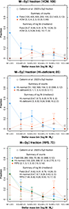 |
Fig. A.1. Stellar mass-Sy2 fraction relation based on mid-infrared colour diagnostics (mIRdds) using central apertures. Environmental classifications follow Section 2.1. Stellar masses are binned as log (M*/M⊙), M1 ≤8.5, 8.5< M2 ≤9.0, 9.0< M3 ≤9.5, 9.5< M4 ≤10.0, 10.0< M5 ≤10.5, and 10.5< M6. Sy2 observed fractions for VCM, H I-deficient, and RPS galaxies are shown alongside median values from 100 stellar mass-matched bootstrap samples of field and H I-normal galaxies (see Section 4.2). Each panel includes galaxy counts, totals and fractions, and median stellar masses, for both bootstrap and original samples. WHAN-based Sy2 fractions from Cattorini et al. (2023) are overplotted for comparison. For original data and bootstrap medians, random uncertainties are expressed as the ratio of the square root of each Sy2 count to the total. |
Appendix B: Reliability of the W3 and W4 band fluxes
To evaluate the reliability of our mid-infrared fluxes, we compare our W3 and W4 integrated measurements with those from Ciesla et al. (2014), who performed integrated WISE photometry for HRS galaxies using manually defined apertures. To convert counts to flux density, Ciesla et al. (2014) used the conversion factors from the Explanatory Supplement to the WISE Preliminary Data Release Products. While they lack measurements for four galaxies, we miss only one, yielding 318 objects with comparable W3 and W4 fluxes. Our data do not include corrections for extended sources, which account for the WISE calibration method, the spectral signature of the source, and an error in the W4 relative system response.
Our W4 integrated fluxes show strong agreement (see Fig. B.1, bottom). The first, second, and third quartiles of the distribution of offsets are −0.015, 0.005, and 0.020 dex, respectively, with a mean offset of −0.049 dex and a standard deviation of 0.254 dex. However, our W3 fluxes are systematically lower (see Fig. B.1, top). The first, second, and third quartiles of the offset distribution are −0.130, −0.106, and −0.058 dex, respectively, with a mean offset of −0.106 dex and standard deviation of 0.163 dex. As a result, our W3−W4 colour indices are redder by a mean of 0.065 dex, with a standard deviation of 0.186 dex.
Despite attempts of using the W3-band labelled pixels for flux extensions and of lowering our detection threshold (4.5 × σ), our W3 fluxes never increased sufficiently to match those of Ciesla et al. (2014). To assess the impact on the excitation classification, we do the exercise of adjusting W3 fluxes upwards by 0.106 dex. The resulting mIRdds show shifts in W3−W4 and W2−W3 colours (towards bluer and redder values, respectively), leading to increased SFG and nd fractions and decreased Sy2 and LINER fractions in mIRdd I. Increments range from a factor of 1.41 to 1.79, while decrements are more constrained, ranging from 0.63 to 0.66. In mIRdd II, a fraction of LINERs classified before as retired galaxies are reclassified as true LINERs, while red LINERs and many Sy2s shift to either nd or SFG types.
Finally, we recalculated excitation-type fractions across the stellar mass bins (as in Table 2), confirming that the modified indices do not alter our original results.
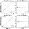 |
Fig. B.1. Comparison of W3 and W4 band integrated fluxes from Ciesla et al. (2014) and this work for 318 HRS galaxies (top and bottom, respectively, with grey points and green line fits). All fits are derived from orthogonal distance regression. Left column: Spearman and Pearson correlation coefficients (ρS, rP, top), and fit slope and intercept (s, i, bottom). Bars show the typical dispersion (interquartile ranges). Right column: flux offsets with the corresponding dispersion (σodr). Red dotted lines indicate the one-to-one relation and zero offset (left and right). |
Appendix C: A comparison with optical line-emission diagnostics
Gavazzi et al. (2018) provide a nuclear classification of HRS galaxies based on spectra collected from the literature and additional observations using the Loiano 1.52 m telescope. They employ the BPT and WHAN diagnostic diagrams. Among their findings, the fraction of H II regions is strongly anticorrelated with stellar mass, in contrast to the increasing frequency of AGNs (including transition objects). Furthermore, they report no significant environmental dependence for AGN activity.
Boselli et al. (2022) similarly report a WHAN classification of the nuclear activity for their compiled RPS galaxy sample. However, both the BPT and WHAN methods rely on optical emission lines, which can be affected by dust attenuation and underlying stellar absorption.7 In the case of Gavazzi et al. (2018), low S/N ratios limited robust BPT classifications, and galaxies they classified as passive (exhibiting only absorption lines) or post-starburst (showing Balmer absorption lines) were assigned these designations via visual inspection of the spectra.
Compared to the BPT, the WHAN diagram has advantages: it requires only the adjacent [N II] and Hα lines and the EW(Hα), and it distinguishes between star-forming (H II region-like), strong and weak AGNs (typically associated with Sy2 and LINER, respectively), and retired systems (including passive and post-starburst types). For these reasons, our comparison focuses solely on WHAN-based classifications.
Gavazzi et al. (2018) provide WHAN classifications for 286 of 323 HRS galaxies (see Table D.1).8 The remaining 36 objects were assigned a posteriori (34 as passive, 2 as post-starburst). Due to WISE data incompleteness, we exclude two galaxies (HRS 116 and 265), leaving 285 galaxies for comparison. For the RPS sample, nuclear classifications are only available for 67 galaxies from Boselli et al. (2022) (see Table D.2), as those compiled by Tiwari et al. (2025) lack the WHAN-based diagnostic.
Table C.1 presents a comparison of excitation type counts between the WHAN method and our mid-infrared diagnostics (mIRdds). For HRS galaxies, the AGN fractions are remarkably consistent across both methods, suggesting that AGN classification is robust to the choice of diagnostic. However, the fractions of SFG and retired types differ by approximately 0.2, with mIRdds typically favouring retired over SFG classes.
A similar trend is observed in the RPS sample, where the mIRdds produce lower SFG and higher retired excitation counts relative to WHAN results (H II and RET, respectively). Consequently, adopting WHAN-based classifications would further amplify the prevalence of star-forming excitation relative to other types.
To test the variability of SFG and retired classes, we apply a modified diagnostic scheme using a higher slope for the AGN/SFG separation (following Coziol et al. 2014, 2015) and a more conservative star-forming cut (from Cluver et al. 2014). These adjustments result in a significant reclassification of Sy2 and retired galaxies as SFG types increase in both HRS and RPS samples to match the WHAN counts (see Table C.1, third column). Notably, LINER counts remain almost unchanged, with the modifications primarily affecting Sy2 and retired excitation types.
It is important to note that Gavazzi et al. (2018) use modified WHAN thresholds, moving rightwards the vertical division between H II region-like and AGN types, and downwards the horizontal boundary separating H II region-like/weak AGNs (wAGNs) from retired (RET) galaxies (see Gavazzi et al. 2011). These changes may tend to increase the number of H II region-like classifications while reducing RET ones.
Finally, the retired excitation category encompasses both RET and passive types. In contrast, the RET class of Gavazzi et al. (2018) refers specifically to galaxies ionized by old stellar populations that may still exhibit weak emission features. In our framework, the retired category also includes systems with neither SF nor emission lines.
Comparison of total counts (fractions) of excitation types.
Appendix D: Mid-infrared photometry of the HRS and the RPS sample
Table D.1 (available in full online) presents the computed mid-infrared photometry (band flux densities) for the HRS galaxies (a total of 321, see Boselli et al. 2010). Similarly, Table D.2 (available in full online) lists the computed photometry for the RPS galaxy sample (a total of 79, see Boselli et al. 2022; Tiwari et al. 2025).
(Available in full online) Mid-infrared photometry (flux densities in mJy) for the HRS sample.
(Available in full online) Mid-infrared photometry (flux densities in mJy) for the RPS sample.
All Tables
(Available in full online) Mid-infrared photometry (flux densities in mJy) for the HRS sample.
(Available in full online) Mid-infrared photometry (flux densities in mJy) for the RPS sample.
All Figures
|
Fig. 1. Examples of background estimation in the W3 band: ESO137-001 (top) and NGC4303-HRS114 (bottom). From left to right, the background level and background-subtracted images are shown, illustrating the selected integrated and central apertures from object detection (red ellipses). Pixel value scales are shown on the right. The green contour levels correspond to 2, 3, 5, and 10 times the representative standard deviation, computed from the selected rectangular regions. |
| In the text | |
|
Fig. 2. Top: mIRdds for 257 late-type HRS galaxies (Boselli et al. 2010). Bottom: mIRdds for 72 late-type RPS galaxies (Boselli et al. 2022; Tiwari et al. 2025). All photometry is based on central apertures (median size ∼3.12 kpc for the HRS; see Section 3.1.4 and Appendix D). Left: mIRdd I (Coziol et al. 2014, 2015), with diagonal divisions separating AGN from SFG excitation, and between levels of SF (diagonal magenta and gold lines and bold labels, respectively). Excitation-type counts are listed at the bottom right. Right: mIRdd II (e.g. Jarrett et al. 2011; Mateos et al. 2012; Caccianiga et al. 2015; Herpich et al. 2016), featuring horizontal thresholds (dotted and dashed magenta lines and bold labels, aided by arrows) and the AGN wedge (magenta polygon) as defined by Stern et al. (2005, 2012), and Mateos et al. (2012). Coloured geometric labels for excitation types assigned in mIRdd I are consistently maintained in mIRdd II to ensure direct comparison and the derivation of a unified classification scheme across diagrams. Common features in both mIRdds as follows. The dashed brown line and bold labels mark the SFG-Retired galaxy divisor (Herpich et al. 2016). Dashed coloured contours represent 0.1 kernel density levels. The grey curve traces the model colour sequence for power-law spectra with annotated spectral indices (Wright et al. 2010, the K-dwarf star colour, K, is also plotted), illustrating the non-thermal radiation trend. Colours redden as the spectral index decreases, distinguishing galaxies (intrinsically redder) from stars (bluer). This sequence also reinforces the characteristic negative spectral indices of AGNs. |
| In the text | |
|
Fig. 3. Stellar mass-excitation fraction relation. Excitation types are based on mid-infrared colour diagnostics (mIRdds) representing central apertures (median size ∼3.12 kpc for the HRS). Section 2.1 details the HRS environmental classification. Stellar masses are binned from low to high (left to right): log (M*/M⊙), M1 ≤ 8.5, 8.5 < M2 ≤ 9.0, 9.0 < M3 ≤ 9.5, 9.5 < M4 ≤ 10.0, 10.0 < M5 ≤ 10.5, and 10.5 < M6. Top: Field and H I-normal galaxies. Middle: Virgo cluster members (VCMs) and H I-deficient galaxies. Bottom: Objects undergoing RPS in nearby clusters. Total galaxy counts are shown in the panel titles. Each panel lists excitation-type counts per mass bin (from left to right), with total counts and respective fractions shown on the rightmost side. The x axis labels indicate galaxy counts per stellar mass bin (top). Random uncertainties, indicated by vertical bars, are expressed as the ratio of the square root of each excitation-type count to the total. See also Tables 2, D.1, and D.2. |
| In the text | |
|
Fig. A.1. Stellar mass-Sy2 fraction relation based on mid-infrared colour diagnostics (mIRdds) using central apertures. Environmental classifications follow Section 2.1. Stellar masses are binned as log (M*/M⊙), M1 ≤8.5, 8.5< M2 ≤9.0, 9.0< M3 ≤9.5, 9.5< M4 ≤10.0, 10.0< M5 ≤10.5, and 10.5< M6. Sy2 observed fractions for VCM, H I-deficient, and RPS galaxies are shown alongside median values from 100 stellar mass-matched bootstrap samples of field and H I-normal galaxies (see Section 4.2). Each panel includes galaxy counts, totals and fractions, and median stellar masses, for both bootstrap and original samples. WHAN-based Sy2 fractions from Cattorini et al. (2023) are overplotted for comparison. For original data and bootstrap medians, random uncertainties are expressed as the ratio of the square root of each Sy2 count to the total. |
| In the text | |
|
Fig. B.1. Comparison of W3 and W4 band integrated fluxes from Ciesla et al. (2014) and this work for 318 HRS galaxies (top and bottom, respectively, with grey points and green line fits). All fits are derived from orthogonal distance regression. Left column: Spearman and Pearson correlation coefficients (ρS, rP, top), and fit slope and intercept (s, i, bottom). Bars show the typical dispersion (interquartile ranges). Right column: flux offsets with the corresponding dispersion (σodr). Red dotted lines indicate the one-to-one relation and zero offset (left and right). |
| In the text | |
Current usage metrics show cumulative count of Article Views (full-text article views including HTML views, PDF and ePub downloads, according to the available data) and Abstracts Views on Vision4Press platform.
Data correspond to usage on the plateform after 2015. The current usage metrics is available 48-96 hours after online publication and is updated daily on week days.
Initial download of the metrics may take a while.