| Issue |
A&A
Volume 703, November 2025
|
|
|---|---|---|
| Article Number | A250 | |
| Number of page(s) | 9 | |
| Section | Cosmology (including clusters of galaxies) | |
| DOI | https://doi.org/10.1051/0004-6361/202555933 | |
| Published online | 19 November 2025 | |
Detection of colour variations from gravitational microlensing observations in the quadruple quasar HE0435-1223: Implications for the accretion disc
Astronomisches Rechen-Institut, Zentrum für Astronomie der Universität Heidelberg, Mönchhofstrasse 12-14, 69120 Heidelberg, Germany
⋆ Corresponding author: This email address is being protected from spambots. You need JavaScript enabled to view it.
Received:
13
June
2025
Accepted:
9
September
2025
Abstract
Aims. We present monitoring observations of quasar microlensing in the quadruple quasar HE0435-1223. The microlensing-induced light curves of the quasar images are chromatic, i.e. they depend on the applied filter band. Comparison with microlensing simulations allows us to infer properties of the accretion disc.
Methods. We determined the R and V band light curves of the four images of HE0435-1223 from 79 and 80 epochs, respectively, taken from 2014 to 2024 at the Las Cumbres Observatory using difference imaging analysis. We considered difference light curves to remove the intrinsic quasar variability. This reveals a prominent, long-term chromatic microlensing event in image B. We used microlensing light curve simulations with both Gaussian and standard thin accretion disc brightness profiles to analyse this signal.
Results. The particularly strong signal observed in image B of HE0435-1223 makes it possible to detect the size ratio of the accretion disc in the R to the V band of 1.24+0.08−0.20 and 1.72+0.11−0.22 for the Gaussian and the thin disc model, respectively. These values are in agreement with standard thin disc theory. For the absolute size, we find large disc half-light radii of around 0.7–1.0 Einstein radii with an uncertainty of about 0.6 dex (depending on the filter bands and the models). Finally, our calculations show that image B undergoes caustic crossings about once per year.
Key words: accretion / accretion disks / gravitational lensing: micro / quasars: individual: HE0435-1223
© The Authors 2025
 Open Access article, published by EDP Sciences, under the terms of the Creative Commons Attribution License (https://creativecommons.org/licenses/by/4.0), which permits unrestricted use, distribution, and reproduction in any medium, provided the original work is properly cited.
This article is published in open access under the Subscribe to Open model. This email address is being protected from spambots. You need JavaScript enabled to view it. to support open access publication.
1. Introduction
In the current picture of the structure of quasars, matter is accreted onto super-massive black holes in the centres of galaxies. Over the past decades, the field has become quite mature (see e.g. Antonucci 1993; Frank et al. 2002; Padovani et al. 2017); however, obtaining direct constraints on accretion disc properties – such as size, brightness profile, or temperature profile – remains challenging. The widely used thin accretion disc model by Shakura & Sunyaev (1973) predicts a power-law temperature profile of the accretion disc following
 (1)
(1)
for sufficiently large radii r ≫ rin outside the inner edge of the disc (here we ignore the inner cut-off term as well as different exponents, see e.g. Abramowicz et al. 1988; Mediavilla et al. 2015; Vernardos et al. 2024). While there are important constraints from reverberation mapping (e.g. Horne et al. 2021, and references therein), direct observational tests of the accretion disc are difficult, since we typically cannot resolve the central quasar regions. However, quasar microlensing offers a way to ‘zoom’ in.
Strong gravitational lensing creates multiple images of a quasar located (from the observer’s point of view) behind a massive galaxy acting as a gravitational lens. The first discovery of such a lensed quasar was the doubly imaged quasar Q0957+561 (Walsh et al. 1979), and over 230 of these objects are confirmed today (Ducourant et al. 2018). By observing light curves (brightness as a function of time) of the multiple images and correcting for the time delays (due to the different light travel paths) between the images, two types of brightness variations can be distinguished: (1) Correlated brightness variations that occur in all images and are intrinsic to the quasar. (2) Brightness variations that occur only in individual images and thus do not originate from the quasar itself. These uncorrelated brightness variations are caused by compact objects in the light path, such as stars in the lensing galaxy near the line of sight to a quasar image. The compact objects exert an additional lensing of the quasar images with deflection angles on the scale of micro-arcseconds. Through the relative motion of the quasar, lens, and observer, a time-varying magnification acts on the quasar images over time scales of weeks, months, and even longer, leading to these uncorrelated brightness variations (see Chang & Refsdal 1979; Schmidt & Wambsganss 2010; Vernardos et al. 2024). This so-called quasar microlensing effect was first detected in the quadruply imaged quasar Q2237+0305 (Irwin et al. 1989; Corrigan et al. 1991), a source discovered by Huchra et al. (1985) and also known as the ‘Einstein Cross’.
Microlensing signals can be used to test model predictions for the structure of quasar accretion discs, such as their size (Kochanek 2004; Poindexter & Kochanek 2010; Morgan et al. 2010, 2018; Cornachione et al. 2020a). The effect of microlensing in the plane of the quasar (source plane perpendicular to the line of sight) can be described by a pattern of varying magnification with characteristic caustic lines (lines of formal infinite magnification) produced by the combined effect of the compact objects (e.g. Kayser et al. 1986; Wambsganss et al. 1990). The microlensing signal depends on the size of the source as it moves through the caustic pattern and averages the magnifications over its size according to the brightness profile. Importantly, this means that the slope of the accretion disc temperature profile is also accessible (Wambsganss & Paczynski 1991; Anguita et al. 2008; Eigenbrod et al. 2008; Poindexter et al. 2008; Mosquera et al. 2009; Cornachione et al. 2020b), since observing the microlensing events in different filters corresponds to the microlensing of different source sizes, where the disc size depends on the filter wavelength according to
 (2)
(2)
assuming that at all radii the accretion disc radiates as a black body with temperature given by Eq. (1).
In a previous study (Sorgenfrei et al. 2024), we described our method to obtain long-term light curves of multiply imaged quasars using point-spread-function (PSF) photometry on images generated with difference imaging analysis (DIA), where we used Gaia proper motion data (Gaia Collaboration 2016, 2023) to improve image alignment and quasar image positions. In that study we applied this method to observations in the R and V band taken at the Las Cumbres Observatory (LCO1, Brown et al. 2013) of the three lensed quasars HE1104-1805, HE2149-2745, and Q2237+0305 and determined their light curves from 2014 to 2022. We have since updated their light curves to include data up to March 2024 and additionally reduced LCO data of another lensed quasar, HE0435-1223, leading to light curves of each image of the four quasars in both bands over ten years2. In this paper we focus on HE0435-1223, utilising the light curve data in both bands to determine constraints on the accretion disc temperature profile.
HE0435-1223 is a quadruply imaged quasar discovered by Wisotzki et al. (2002). The four images are observed in a ‘cross’ configuration similar to the Einstein Cross with comparatively wide separations (see Table 1). The quasar is located at a redshift zs = 1.693 (Sluse et al. 2012). It is lensed by a foreground galaxy at zL = 0.454 (Eigenbrod et al. 2006), which can be seen in Hubble Space Telescope (HST) images (Falco et al. 2001) but is not very prominent in our observations (see inset on the left panel in Fig. 1). The time delays between the images, as determined by COSMOGRAIL, are ΔtAB = (−9.0 ± 0.8) days,  , and ΔtAD = (−13.8 ± 0.8) days, where image A is leading (Millon et al. 2020).
HE0435-1223 image position separations.
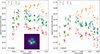 |
Fig. 1. Light curves of HE0435-1223. This figure shows the time-delay-corrected light curves of the four images of HE0435-1223 in the R band (left) and V band (right) with the same time and magnitude ranges, with 1σ magnitude errors. Inside the left panel, we inserted the DIA reference image of HE0435-1223 in the R band (linear in flux) as an example. The image size is 9 arcsec × 9 arcsec. Quasar image A is on the right, and images B, C, and D follow clockwise. Here, image B appears to be the brightest, since the R band reference image is combined mostly from images from the year 2022. |
We summarise the main steps of the data reduction with the resulting light curves in Sect. 2 and present the microlensing signal we found. In Sect. 3 we describe a set of microlensing simulations to investigate this signal. We present and discuss our results in Sect. 4 and conclude in Sect. 5.
2. From LCO data to microlensing signal
In order to investigate quasar microlensing, we used R and V band data taken at LCO, a global network of robotic telescopes. Targeting multiple lensed quasars, data have been acquired since 2014 by 1 m telescopes at five locations (mainly Cerro Tololo, Chile3; but also: Sutherland, South Africa; Siding Springs, Australia; McDonald, USA; and Teide, Spain), with a total of 677 and 697 observations of HE0435-1223 between July 24, 2014, and January 17, 2024 (many during a single night) in the R and V bands, respectively. Since the method to reduce the data and determine the light curves is the same as in Sorgenfrei et al. (2024), we only summarise the main steps in the following subsection and refer to our previous paper for the implementation4 and further details.
2.1. Data reduction
Each observation was aligned to a reference image using the alignment routine of the ISIS software5 by Alard (2000). We modified it to include Gaia proper motion data to improve the alignment by correcting the determined star positions in the reference image according to their proper motion and the time between observation and reference image. For HE0435-1223, the median dispersion of star position deviations between observation and reference image after image alignment (see Eq. (2) in Sorgenfrei et al. 2024) improved from ⟨σ⟩∼59 mas before to ∼43 mas after this Gaia correction. Afterwards, images from one night were combined, leaving us with 79 epochs in the R band as well as 80 in the V band. We additionally produced a high S/N reference image from a few low-seeing observations for the DIA (see inset on the left panel of Fig. 1).
In preparation for applying the DIA method, we used PSF photometry to determine the positions of quasar image A in the combined images and the PSFs, as done in Giannini et al. (2017). For this step, we used GALFIT (Peng et al. 2002, version 2.0.3) modified to fit a multiple quasar image model consisting of copies of the PSF (a fixed 30 × 30 pixel cutout of a star in the vicinity of the quasar) with fixed relative positions determined from HST images. For HE0435-1223 the fixed separations are given in Table 1. Applying this model to each of our combined images, GALFIT finds the best value for the position of quasar image A.
Next, DIA was applied to all images to obtain the difference between each combined image and the reference image. In detail, for each combined image, the reference image was convolved with a continuous kernel function estimated from 5 × 5 stamp stars scattered across the entire image to correct for seeing differences. This was done using the so-called hotpants software6 by Becker (2015), an implementation of the algorithm from Alard & Lupton (1998) and Alard (2000). The resulting difference images contain only brightness variations with respect to the reference image. Therefore, light from the lens galaxy was removed, and only brightness variations of the four quasar images remain at their positions.
Finally, the quasar light curves were extracted from the difference images by applying PSF photometry at the position of quasar image A of our multiple quasar image model with the PSF fixed from before. The resulting difference fluxes were then added to the quasar image fluxes obtained from PSF photometry of the reference image. The zero point of the apparent magnitude scale was determined by the brightness of several stars in the R and V band reference images relative to their apparent magnitudes determined from GaiaG, Gbp, and Grp data (see Riello et al. 2021).
2.2. Light curves of HE0435-1223
The final light curves (apparent magnitudes over time) are shown in Fig. 1 and consist of 79 and 80 data points for all four images in the R and the V band, respectively. The light curves of images B, C, and D are shifted in time by the delays given in Sect. 1. The intrinsic quasar variability is clearly visible in all images and both bands, with the brightness peaks around 2019 and in 2022, as well as the general shape of the curves, except for the strong increase in brightness of image B compared to the other images. Over the ten years of observations, the apparent magnitude of image B changes by up to ∼1.0 mag in the R band and ∼1.3 mag in the V band.
2.3. Difference curves and microlensing signal
We interpret that the additional variability of image B noticeable in Fig. 1 is due to microlensing, as described in Sect. 1. In order to isolate this additional microlensing signal quantitatively, we calculated difference curves between pairs of observed light curves. This removed the intrinsic quasar variability present in all images. Since the light curves of the individual images must be corrected for time delays, interpolation between data points is required to calculate this difference. This can sometimes be problematic for time delays for which the shifted light curve is moved into seasonal observation gaps of the other light curve. However, the time delays of HE0435-1223 are of the order of just a few days (Millon et al. 2020, see Sect. 1), resulting in only slightly shifted light curves with substantial overlap and no need for uncertain interpolation across data gaps.
We used linear interpolation of image A to the time-delay-corrected epochs of images B, C, and D, as well as from B to C and D, and finally C to D. Interpolation was only done between data points separated by ≤30 days. Errors of the interpolated light curves were estimated using Monte Carlo sampling, assuming Gaussian errors of the data points. The difference curves were then computed as the differences between a given reference light curve and the suitably interpolated light curve; for example, B − A := mB(t + ΔtAB)−mA, interp.(t), with standard Gaussian errors. The resulting six difference curves are shown in Fig. 2.
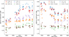 |
Fig. 2. Difference curves of HE0435-1223. Shown are the six combinations of differences of the four light curves (B − A, C − A, and D − A on the left side, and C − B, D − B, and D − C + 1.0 mag on the right side) both in the R band (red circles, orange diamonds, and brown squares) and the V band (blue crosses, violet dots, and green minuses) with 1σ uncertainties. |
In all three combinations of difference light curves including image B, the above mentioned strong microlensing variation can be seen. A colour effect is also visible: the variation has a larger amplitude in the V band than in the R band. However, the three combinations using image A show an additional long-term microlensing signal in the form of an approximately linear rise, which indicates that the B − A curve includes the combination of microlensing signals from two lines of sight and is thus more difficult to analyse (e.g. Eigenbrod et al. 2008; Anguita et al. 2008). Nevertheless, the difference between images C and D (bottom curve in the right-hand panel of Fig. 2) is mostly flat, implying no (or little) microlensing in these images. This makes the C − B (or D − B) curve a suitable target for a microlensing analysis, with the microlensing signal coming chiefly from one line of sight. Consequently, we restrict our microlensing analysis to the signal in the (inverted) B − C curve, thus avoiding the combinatorial explosion arising from a necessity of simulating microlensing in all images simultaneously (e.g. Kochanek 2004). We repeated the simulation described in Sect. 3 and the subsequent analysis in Sect. 4, using the B − D curve (which is affected more by noise, since image D is fainter). The results are consistent, albeit with slightly larger uncertainties.
3. Microlensing simulations
In order to quantitatively analyse the (chromatic) microlensing signal of image B in the difference curve B − C, we simulated microlensing light curves and compared them to our data, mainly following the method developed in Kochanek (2004), which has been used in subsequent studies to analyse microlensing in several lensed quasar systems (e.g. Anguita et al. 2008; Morgan et al. 2010, 2018; Cornachione et al. 2020a,b).
3.1. Magnification patterns
First, source-plane magnification patterns with the microlensing parameters of image B were generated using Teralens7 (Alpay 2019). It is a new implementation of the inverse ray shooting tree code from Wambsganss (1999), fully parallelised for GPUs. We fixed the total convergence and shear to κ = 0.539 and γ = 0.602 (Schechter et al. 2014) and varied the fraction of compact matter κ⋆ in steps of 0.1 from κ⋆/κ = 0.1 to 1.0 (the convergence is composed of contributions from compact and smooth matter κ = κ⋆ + κsmooth, as usual). We assumed equal masses of M = 1M⊙ for all microlenses in the lens plane (Lewis & Irwin 1996) and produced ten statistically independent magnification patterns with sizes of 40 RE × 40 RE and a resolution of 200 pixel/RE. Using a flat cosmology with H0 = 70.0 kms−1 Mpc−1, Ωm, 0 = 0.3, and the redshifts from Sect. 1, the source-plane Einstein radius (which scales with the square root of the true mean mass ⟨M⟩ of the microlenses) corresponds to
 (3)
(3)
where DS, DL, and DLS are the angular diameter distances from observer to source, observer to lens, and lens to source.
As mentioned in Sect. 1, the apparent source size connected to the quasar’s temperature profile influences the observed microlensing signal, which is the focus of this study. Inserting the temperature profile (Eq. (1)) of a quasar from the thin disc model (Shakura & Sunyaev 1973) into Planck’s law (assuming a small filter width) results in a radial surface brightness profile
![Mathematical equation: $$ \begin{aligned} B(r) \propto \left[\exp \left(\left(\frac{r}{r_s}\right)^{3/4}\right)-1\right]^{-1}, \end{aligned} $$](/articles/aa/full_html/2025/11/aa55933-25/aa55933-25-eq7.gif) (4)
(4)
with a characteristic scale radius rs where the temperature T(rs) = hc/(kBλ0) matches the filter wavelength in the quasar rest frame λ0. However, this profile is often replaced with a Gaussian brightness profile
 (5)
(5)
with a (different) scale radius Rs. This can be used instead, since Mortonson et al. (2005) showed that primarily the overall size measured in half-light radii r1/2 is important for the microlensing effect, rather than the detailed shape of the radial profiles. Integrating the profiles, assuming circular symmetry, results in half-light radii of r1/2 ≃ 2.44rs for the Shakura-Sunyaev thin disc profile (Eq. (4)) and r1/2 ≃ 1.18Rs for the Gaussian disc (Eq. (5)), both viewed face-on.
Nevertheless, we considered both types of profiles in this study. We produced circularly symmetric kernels (extending out to 10 scale radii, or at most 10 RE) as a model for the brightness of face-on quasar accretion discs. We therefore convolved our 10 (κ⋆/κ varying) magnification patterns for image B with these kernels made from 80 different scale radii values for both the Shakura-Sunyaev thin disc and the Gaussian brightness profile, in total yielding 1600 convolved maps.
The 80 size values were chosen non-logarithmically over a large range, resulting in an approximately even sampling of size ratios (see Anguita et al. 2008; Eigenbrod et al. 2008, more on this in Sect. 4). We tested the same size values as the scale radius parameter for both the thin disc rs and the Gaussian disc Rs, starting with 0.5, 1, 2, 3, 4, 6, 8, and 10 pixels; then continuing in steps of 5 pixels up to 200 pixels, 10 pixel-steps up to 400 pixels, 20 pixel-steps up to 600 pixels, and finally 50 pixel-steps up to 800 pixels. Therefore, we tested discs with scale radii as small as 0.0025 RE and as large as 4.0 RE, corresponding to r1/2 ≃ 0.0029 RE or 0.0056 RE (around the pixel scale) up to r1/2 ≃ 4.71 RE or 8.96 RE for the Gaussian and thin discs half-light radii, respectively. In order to avoid edge effects for the largest discs from the convolution (using a fast Fourier transform, which assumes periodical patterns), we discarded the outer 5 RE on all sides of each convolved magnification map. This left us with convolved magnification patterns of 30 RE × 30 RE.
3.2. Light curve fitting
To extract light curves from the 1600 convolved magnification maps, we constructed 107 tracks with track lengths corresponding to ten years by drawing 107 velocities sampled from a log-uniform distribution between 0.002 RE/yr and 2.0 RE/yr (in principle limited only by the size of our magnification patterns). These tracks had random directions and random x and y start point coordinates (within the central 30 RE × 30 RE, with those leaving this region having their start points redrawn). As an example, in Fig. 3 we show the unconvolved magnification map for κ⋆/κ = 0.8 generated with Teralens together with 200 tracks, showcasing the range of track lengths (i.e. velocities), random directions as well as the restriction to the central 30 RE × 30 RE.
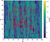 |
Fig. 3. Magnification pattern with example tracks. Shown are the first 200 tracks (in red) on the unconvolved magnification map of image B, as produced by Teralens for κ⋆/κ = 0.8. |
For each compact object fraction κ⋆/κ, each disc size rs or Rs, and both disc models, we placed all tracks on the corresponding map and interpolated the magnitudes of 500 equally spaced steps along each track. The generated light curves were then compared to the R and V band B − C difference curves from Sect. 2.3, by fixing the start time of the simulated tracks to t0 = 2014.5 yr and then interpolating them to the epochs ti of the difference curves, thus extracting two simulated microlensing curves of image B at the same epochs of the R and V difference curves, respectively. Since we assumed no microlensing along the line of sight of image C, we subtracted a constant offset μC (accounting for the mean magnification from strong lensing and a possible non-zero but constant microlensing signal in image C) from each simulated μB(ti) curve. The offset μC was chosen such that the difference of the mean magnitude values of simulated and measured difference curves was minimised. The resulting goodness-of-fit estimator χ2 is
![Mathematical equation: $$ \begin{aligned} \chi ^2 = \sum _i\left[\frac{\mu _B(t_i)-\mu _C-(B-C)(t_i)}{\sigma _i}\right]^2, \end{aligned} $$](/articles/aa/full_html/2025/11/aa55933-25/aa55933-25-eq9.gif) (6)
(6)
which is essentially Eqs. (6) and (7) of Kochanek (2004) applied to our case, with the σi set to the magnitude errors of B − C at epochs ti, where we added 0.05 mag in quadrature to the 1σ errors of both light curves analogous to Kochanek (2004). Subsequent studies have similarly incorporated unknown systematic uncertainties (e.g. Eigenbrod et al. 2008; Poindexter & Kochanek 2010; Morgan et al. 2018). This remains likewise necessary for our simulations, because our microlensing model does not explain these remaining residuals (see e.g. Paic et al. 2022, for a recent discussion of possible implications).
In all 108 cases (107 tracks on ten independent maps) and for both models, we determined the best-fitting disc size of all 80 tested sizes that minimises χ2 from Eq. (6). This was done independently for R and V, and since we wanted our simulated light curves to reproduce both the R and V band data, we added these best-size χR2 and χV2 values to a combined χ2 = χR2 + χV2. This results in a χ2 value with a best disc size in R and V for each of the 107 × 10 tracks and for both disc models.
These χ2 values were then converted to ‘track probabilities’ P(χ2), the likelihood of each simulated R and V band light curve pair, using Eq. (10) from Kochanek (2004)8. We applied this procedure only to tracks for which χred2 ≤ 5 holds for the reduced χred2 = χ2/Nd.o.f., speeding up the computations by removing models with vanishing likelihood. Finally, these results were collected in a ‘track library’ including track number, κ⋆/κ, velocity, direction, the four best sizes, and the two track probabilities. About 22.9% of all 107 × 10 tracks have non-vanishing track probabilities for the best-size estimates in the R and V band for either the thin disc model, Gaussian disc model, or both disc models. Our Python code to simulate the light curves, calculate χ2-values, and produce the track library is available as well9.
4. Results and discussion
In Fig. 4, we show the 25 best-fitting (in terms of track probability from Sect. 3.2) simulated light curves in R and V, together with the observed B − C data points, for the Gaussian (left panel) and the thin disc model (right panel). For both disc models, it is noticeable that for almost all tracks the best-fitting simulated V band model shows larger variations than the corresponding R band model. This result is consistent with the expected outward-decreasing temperature profile from the theory of accretion discs (Sect. 1) and corresponds to a relative difference of the measured disc sizes in the R and V band (with smaller discs in the V band), since larger sources show lower amplitude microlensing variations. Note that only two of each 25 best-fitting tracks are identical for both disc models. Also, the shapes of the light curves from the two models appears different, with more numerous and sharper variations in the thin disc model, hinting at subtle differences between the two models. We stress that, in the following section, we consider all library tracks in our analysis.
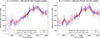 |
Fig. 4. Best-fitting simulated light curves. We show here the best-fitting R and V simulated microlensing light curves (red and blue curves) from the 25 tracks with the smallest χ2 = χR2 + χV2 for the Gaussian disc model (left) and the Shakura-Sunyaev thin disc model (right). The data points are the measured R (orange circles) and V (purple squares) B − C difference curves (i.e. the two uppermost curves on the right side of Fig. 2 inverted and with adapted error bars as described in Sect. 3.2) as used for the χ2 calculation. |
4.1. Size ratio and accretion disc temperature profile
For each of the 108 tracks in our library, we can determine the ratio of the source size in the R and V band. This size ratio qR/V is directly related to the temperature profile (Eq. (1)) via an observed size dependence on the wavelength (Eq. (2)) of a Shakura-Sunyaev disc as discussed in Sect. 1. For the central filter wavelengths λc(R) = 6407 Å and λc(V) = 5548 Å (Bessell 2005), the expected theoretical size ratio therefore is  (i.e. a Shakura-Sunyaev disc is expected to appear 24.1% larger in radius in the R band than in the V band).
As mentioned in Sect. 3.1, we chose 80 different scale radius values non-logarithmically spaced, similar to Anguita et al. (2008) and Eigenbrod et al. (2008). These were selected such that the resulting size ratios were as densely and close to evenly distributed in the ratio-space as possible. Therefore, for each track, we computed the best-fitting R band over V band half-light radii fraction qR/V := r1/2(R)/r1/2(V) for the Gaussian and the thin disc model. We constructed the histogram for qR/V by summing over the track probabilities P(χ2) for a given size ratio bin (we used 16 ratio bins from 0.7 to 2.2 in steps of 0.1). However, these bins were not exactly evenly sampled by the possible ratios. We corrected for this by normalising the probabilities by the number of source size combinations contributing to a particular bin. Overall, this is a minor correction since we selected the source sizes such that all their possible ratios were distributed as evenly as possible.
In Fig. 5, we present the half-light radii ratio distributions P(qR/V) for both disc models. The mean values with 1σ uncertainties are  for the Gaussian disc model and
  for the thin disc model, both consistent with each other and the theoretically expected value. It can be noted, however, that the thin disc model prefers a somewhat larger ratio value, which corresponds to a shallower temperature profile according to Eq. (1), with a negative exponent closer to β = 1/2 (but still in agreement with β = 3/4 from standard thin disc theory)10. Such shallower temperature profiles have been measured and predicted as well as used to explain the typically observed size discrepancy, with the disc appearing larger in microlensing studies than expected from their luminosity (Poindexter et al. 2008; Morgan et al. 2010, 2018; Li et al. 2019; Cornachione et al. 2020b; Cornachione & Morgan 2020).
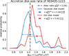 |
Fig. 5. Disc size ratio distribution. Shown are the probability distributions of the size ratio qR/V (ratio of R and V band size) for the Gaussian (blue) and the thin disc model (red) with corresponding mean values (blue circle for the Gaussian and red diamond for the thin disc model), each with 1σ uncertainties. Note that their position along the ordinate is arbitrary. The dash-dotted black line indicates the theoretically expected value. |
Since our standard thin disc simulation concludes with a size ratio consistent with standard thin disc theory but with a tendency toward a shallower β = 1/2 temperature profile, we have run the same simulation again only changing the slope in Eq. (1) to β = 1/2. Interestingly, all results almost perfectly agree with the β = 3/4 simulation, and we find  , close to the expected size ratio of 1.383 for a thin β = 1/2 disc and consistent with the ratio expected from standard theory. Therefore, we cannot distinguish these two models from our analysis.
4.2. Accretion disc size estimates
The distribution of accretion disc sizes in units of Einstein radii can similarly be inferred from our simulation results; for each track in our library, one needs to add the probability corresponding to the best-fitting R and V band half-light radii to the appropriate histogram bins for both disc models. We thus obtained four probability distributions P(r1/2|D) given our data D. From these, we find  for the Gaussian model in the R and
  in the V band, while the thin disc model correspondingly gives
  and
and  . We note that a quasar accretion disc of comparable size has recently been found by Forés-Toribio et al. (2024) in the system SDSS J1004+4112.
Moreover, since each track is associated with a velocity in RE/yr, we constructed probability distributions P(v|D) for both models, with mean track velocities of about 0.48 and 0.33 RE/yr for the Gaussian and the thin disc model, respectively. Combining both size and velocity information, one can identify the well-known linear source size–velocity degeneracy (e.g. Kochanek 2004). We note that we also checked the distributions of the velocity direction and the compact fraction κ⋆/κ. We find only mild but insignificant trends of smaller χ2 values towards velocities non-parallel to the shear direction and towards maps with higher compact fraction.
One can convert the half-light radii r1/2 (in RE) to absolute sizes in cm by fixing the mean lens mass ⟨M⟩ in Eq. (3). Alternatively, assumptions can be made about the velocities involved (source, lens plane, and observer), which also translate into the mean mass of the compact objects. In fact, a probability distribution of the compact objects can be determined following the Bayesian method described in Kochanek (2004, especially Eqs. (13)–(18)). In brief, a prior effective source velocity probability P(ve) is constructed (with ve in km/s) and convolved with the velocity likelihood function P(v|D) from the simulation (with v in RE/yr) to determine a lens mass distribution P(⟨M⟩|D).
P(ve) then combines velocity contributions from the observer with respect to the cosmic microwave background in the lens plane perpendicular to the direction to the quasar, Gaussian estimates for the peculiar velocities of lens galaxy and quasar, as well as the stellar velocity dispersion of the microlenses (see Kayser et al. 1986; Kundic & Wambsganss 1993; Kochanek 2004; Vernardos et al. 2024), resulting in a broad probability density distribution with an average effective velocity of  . The velocity dispersion of the stars in the lens galaxy was measured by Courbin et al. (2011) as σ⋆ = 222 km/s. We integrated the mass distribution P(⟨M⟩|D) together with the half-light radii distribution P(r1/2(⟨M⟩)|D), where we used a constant mass prior from 0.1 to 1.0 M⊙ (Kochanek 2004; Morgan et al. 2018) and obtained a probability distribution for the absolute size of the accretion disc in cm.
To be able to compare the measured sizes to literature values, we converted the r1/2[cm]-values to the R2500[cm] value from Morgan et al. (2010), where the size is expressed in terms of the thin disc scale parameter rs (see Eq. (4) and Sect. 3.1, i.e. dividing the half-light radii by 2.44) at a UV-wavelength in the quasar rest frame of 2500 Å (using Eq. (2)) of an inclined disc (assuming an average inclination angle of i = 60°, which increases the actual disc size by a factor of  ). Therefore, we converted to
![Mathematical equation: $$ \begin{aligned} R_{2500}=\frac{\sqrt{2}\,r_{1/2}}{2.44} \times \left[\frac{{2500}\,{{\AA }}}{\lambda _c/(z_{\rm s}+1)}\right]^{4/3}, \end{aligned} $$](/articles/aa/full_html/2025/11/aa55933-25/aa55933-25-eq20.gif) (7)
(7)
with the central filter wavelength λc (see Sect. 4.1) and the source redshift zs (see Sect. 1). The resulting size distributions P(R2500[cm]) for both models and bands are shown in Fig. 6. We find  for the Gaussian disc in R and
  in V, as well as
  for the thin disc in R and
  in V, i.e. all around R2500 ≃ 2.4 × 1016 cm.
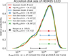 |
Fig. 6. Disc size estimates R2500. Shown are the probability distributions for the accretion disc size of HE0435-1223 from our simulations using the Gaussian disc model with the R band data (in red) and with the V band data (in blue), as well as the thin disc model with R (in orange) and with V (in green). The corresponding data points (in colour), with error bars, show the size expectation values with 1σ intervals. Similarly, the black data point shows the microlensing size result of HE0435-1223 found by Morgan et al. (2010). Note that the position of the data points along the ordinate is arbitrary. |
For comparison, we note that Morgan et al. (2010) found an accretion disc size of  for HE0435-1223 from a microlensing analysis, which is smaller but in agreement with our values. Our microlensing-based disc sizes (as well as their value) are larger than their luminosity-based estimate. In fact, Morgan et al. (2010, 2018) show that such a discrepancy is found in many systems.
4.3. Number of caustic crossings
In the previous section, we derived average velocities of the quasar across the magnification patterns of 0.48 or 0.33 RE/yr for the Gaussian or thin disc, respectively. During the approximately ten years of our observations, the quasar has (on average, approximately) moved three to five Einstein radii, raising the question of how many caustics the quasar has encountered or crossed in this time. Here we count the caustic crossing of the disc centre; caustics that merely touch the outer part of the disc are not included. Consequently, the result is a lower limit that is nevertheless indicative of the number of traversed caustic structures.
We estimate the precise location of the caustics by using the complex parametrisation of caustics by Witt (1990), as implemented in causticfinder-py11. We use the same positions and masses of the microlenses as in Teralens12. We count the number of caustic crossings Ncc (in our case per 10 yr, since this is the length, which the simulated tracks correspond to) by calculating the number of intersections of each track with caustic lines for all tracks in our library with non-zero probability (see Fig. 7a for an example track on the Teralens map together with the caustics calculated with causticfinder-py). Note that not all caustic crossings lead to uniquely identifiable features in the light curves due to the (potentially small) separation along the track in time and the averaging effect from the source size.
Adding again the probabilities of each track in our library to the appropriate bins in a histogram of the number of caustic crossings, we obtain the probability distribution for Ncc shown in Fig. 7b. We find that the expected number of caustic crossings per 10 yr ⟨Ncc⟩ is  and
and  for the Gaussian and the thin disc model, respectively (with 16th and 84th percentiles as uncertainty). This essentially corresponds to around one caustic crossing per year, with a large spread.
The probability of having at least one caustic crossing within the 10 yr interval integrates in both models to about 90%. We stress again that the true number is even higher since we did not include the extent of the disc. Given the size estimate from the last section, this makes caustic crossings in image B of HE0435-1223 very likely at all times. This could be especially interesting for studying this object in the X-ray regime (e.g. Guerras et al. 2017) because not only is the X-ray source expected to be much smaller than the optical continuum region (Pooley et al. 2006; Zimmer et al. 2011), but also the emission from the smallest radii will be magnified most strongly in the X-ray spectra (e.g. Reynolds et al. 2014; Mediavilla et al. 2015; Chartas et al. 2017).
5. Conclusion
We obtained R and V band observations of lensed quasars at the Las Cumbres Observatory (LCO) from the past ten years. From these, we determined light curves of the quasar images by applying DIA (together with PSF photometry and Gaia proper motion data). In this study, we presented light curves of the four images of HE0435-1223 with 79 and 80 epochs in the two bands (Fig. 1). We determined difference curves (Fig. 2) and find a strong microlensing signal in quasar image B.
We proceeded to analyse this signal by comparing with microlensing simulations (Sect. 3) using Teralens for the magnification patterns and the light curve simulation and fitting method developed by Kochanek (2004). We applied our microlensing light curve simulations both to the Shakura-Sunyaev thin accretion disc model (Eq. (4)) and the Gaussian disc model (Eq. (5)). Our analysis (Sect. 4) shows that:
-
The accretion disc is larger in the R than in the V band by a factor of
 in the Gaussian disc model, and by a factor of
  in the thin disc model. This is our main result, made possible only by the observations in two different photometric filters. These size ratios agree with the prediction of thin disc theory (Shakura & Sunyaev 1973), which expects a factor of ∼1.241 between the two bands.
 -
The absolute size of the disc in terms of its half-light radius ranges from 0.7 RE to 1.0 RE (with an uncertainty of about 0.6 dex) for the different models and bands, which we could all consistently convert to about R2500 ≃ 2.4 × 1016 cm in terms of an inclined thin disc scale parameter at λrest = 2500 Å, i.e. larger but still in agreement with the value found by Morgan et al. (2010). In agreement with that study, our disc size measurement is thus also larger than that predicted from their luminosity-based size estimate.
-
Furthermore, we determined that on average (the centre of) image B crosses a caustic roughly once per year, explaining the long-term fluctuations and the amplitude of the microlensing signal we find in the difference curves (Fig. 2).
Our results are consistent between the two disc models, as suggested by Mortonson et al. (2005). We also see small differences, such as the shape of the light curves (Fig. 4) and the marginally different size ratios (Fig. 5). Further studies testing multiple models could be used to find out whether such hints at deviations from the standard Gaussian brightness profile can be identified in other systems as well. Also, since different studies have found temperature profile slopes that deviate from thin disc theory (e.g. Cornachione & Morgan 2020, who conclude, incorporating results from multiple studies, that shallower slopes are favoured), it could be revealing to include models with shallower slopes, such as β = 1/2 (which is also close to the value we find for the thin disc model and therefore tested as described in Sect. 4.1). This is especially the case, since such shallower temperature profiles can be used to explain the accretion disc size discrepancy typically found between large microlensing and smaller luminosity-based estimates (Morgan et al. 2010).
We have updated our LCO light curve data for the three quasars in Sorgenfrei et al. (2024) and are working on more lensed quasars to find suitable chromatic microlensing events to analyse. In the future, multi-band data from the Legacy Survey of Space and Time (LSST) of the Vera C. Rubin Observatory will produce huge amounts of data ideal for chromatic quasar microlensing studies (Ivezić et al. 2019), thereby helping to constrain the structure of quasar accretion discs further.
Data availability
The R and V band light curves of HE0435-1223 from Fig. 1 are available at the CDS via https://cdsarc.cds.unistra.fr/viz-bin/cat/J/A+A/703/A250. The updated light curves of the four quasars described in Sect. 1 are available at GAVO Data Centre (2025).
The updated (and new) light curves of the four quasars (with more to come in the future) are available at GAVO Data Centre (2025), including data up to March 2024. For HE1104-1805, they now consist of 124 R and 126 V band epochs; for HE2149-2745, 175 R and 146 V band epochs; and for Q2237+0305, 115 R and 114 V band epochs, which is an overall increase of ∼39% compared to Sorgenfrei et al. (2024).
For the final light curves of HE0435-1223, only data taken at Cerro Tololo, Chile was used, since a low number of observations from other locations were excluded at various steps in the data reduction.
Teralens is a microlensing code developed by Alpay (2019) for use on graphics processing units (GPUs) available at https://github.com/illuhad/teralens. For reference, we note that the shear direction in Teralens is rotated by π/2 when compared to microlens (Wambsganss 1999). We added the output of the mean magnification to the default version of Teralens to be able to calculate magnitudes.
Therefore, we use P(χ2)∝Γ[Nd.o.f./2 − 1, χ2/(2f02)], which implies a rescaling of χf2 = χ2/f2 with P(f)∝f for 0 ≤ f ≤ f0 (see Kochanek 2004). For our combined R and V band B − C data, the number of degrees of freedom is Nd.o.f. = 98. We set f0 = min(3χred/2), which is of order unity, independently for the thin and Gaussian disc, chosen such that in both cases the minimum rescaled reduced χf2/Nd.o.f. has an expectation value of 1. This allows us to compare the two disc models, even though their χ2 distributions differ slightly.
A direct conversion of the distribution of qR/V values to the often used negative temperature profile slope β (see Eq. (1)) is problematic due to the pole at qR/V = 1. However, the inverse slope ζ = 1/β, monotonically increasing as a function of qR/V, is accessible (similar as in Eigenbrod et al. 2008). We find  , again compatible with thin disc theory where ζ = 4/3, but somewhat shallower.
Note that the definition of the Einstein radius RE in Witt (1990) includes an additional factor of  . The caustics thus determined agree perfectly with the magnification pattern calculated by Teralens, see Fig. 7a.
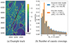 |
Fig. 7. Number of caustic crossings Ncc. On the left, we show an example track (in red) on the κ⋆/κ = 1.0 map (colour map in magnitudes, x- and y-axis in pixels) crossing 11 (marked with black crosses) caustics (in yellow) over the ten simulated years. On the right, we show the resulting histogram of Ncc (curtailed at Ncc = 20) over all library tracks weighted by their probability. |
Acknowledgments
This work makes use of observations from the Las Cumbres Observatory global telescope network. The authors acknowledge support by the High Performance and Cloud Computing Group at the Zentrum für Datenverarbeitung of the University of Tübingen, the state of Baden-Württemberg through bwHPC and the German Research Foundation (DFG) through grant no INST 37/935-1 FUGG. This work has made use of data from the European Space Agency (ESA) mission Gaia (https://www.cosmos.esa.int/gaia), processed by the Gaia Data Processing and Analysis Consortium (DPAC, https://www.cosmos.esa.int/web/gaia/dpac/consortium). Funding for the DPAC has been provided by national institutions, in particular the institutions participating in the Gaia Multilateral Agreement. This work made use of Astropy (http://www.astropy.org). C.S. acknowledges support from the International Max Planck Research School for Astronomy and Cosmic Physics at the University of Heidelberg. We thank Aksel Alpay for support with Teralens, Markus Demleitner for making the data available at GAVO, as well as Markus Hundertmark, Yiannis Tsapras, Zofia Kaczmarek and David Kuhlbrodt for helpful discussions. Finally, we thank the anonymous referee for the helpful report.
References
- Abramowicz, M. A., Czerny, B., Lasota, J. P., & Szuszkiewicz, E. 1988, ApJ, 332, 646 [Google Scholar]
- Alard, C. 2000, A&AS, 144, 363 [NASA ADS] [CrossRef] [EDP Sciences] [Google Scholar]
- Alard, C., & Lupton, R. H. 1998, ApJ, 503, 325 [Google Scholar]
- Alpay, A. 2019, Teralens – A parallel (quasar) microlensing code for multi-teraflop devices, https://github.com/illuhad/teralens [Google Scholar]
- Anguita, T., Schmidt, R. W., Turner, E. L., et al. 2008, A&A, 480, 327 [NASA ADS] [CrossRef] [EDP Sciences] [Google Scholar]
- Antonucci, R. 1993, ARA&A, 31, 473 [Google Scholar]
- Becker, A. 2015, Astrophysics Source Code Library [record ascl:1504.004] [Google Scholar]
- Bessell, M. S. 2005, ARA&A, 43, 293 [NASA ADS] [CrossRef] [Google Scholar]
- Brown, T. M., Baliber, N., Bianco, F. B., et al. 2013, PASP, 125, 1031 [Google Scholar]
- Chang, K., & Refsdal, S. 1979, Nature, 282, 561 [Google Scholar]
- Chartas, G., Krawczynski, H., Zalesky, L., et al. 2017, ApJ, 837, 26 [NASA ADS] [CrossRef] [Google Scholar]
- Cornachione, M. A., & Morgan, C. W. 2020, ApJ, 895, 93 [Google Scholar]
- Cornachione, M. A., Morgan, C. W., Millon, M., et al. 2020a, ApJ, 895, 125 [Google Scholar]
- Cornachione, M. A., Morgan, C. W., Burger, H. R., et al. 2020b, ApJ, 905, 7 [NASA ADS] [CrossRef] [Google Scholar]
- Corrigan, R. T., Irwin, M. J., Arnaud, J., et al. 1991, AJ, 102, 34 [NASA ADS] [CrossRef] [Google Scholar]
- Courbin, F., Chantry, V., Revaz, Y., et al. 2011, A&A, 536, A53 [NASA ADS] [CrossRef] [EDP Sciences] [Google Scholar]
- Ducourant, C., Wertz, O., Krone-Martins, A., et al. 2018, A&A, 618, A56 [NASA ADS] [CrossRef] [EDP Sciences] [Google Scholar]
- Eigenbrod, A., Courbin, F., Meylan, G., Vuissoz, C., & Magain, P. 2006, A&A, 451, 759 [NASA ADS] [CrossRef] [EDP Sciences] [Google Scholar]
- Eigenbrod, A., Courbin, F., Meylan, G., et al. 2008, A&A, 490, 933 [NASA ADS] [CrossRef] [EDP Sciences] [Google Scholar]
- Falco, E. E., Kochanek, C. S., Lehár, J., et al. 2001, ASP Conf. Ser., 237, 25 [Google Scholar]
- Forés-Toribio, R., Muñoz, J. A., Fian, C., Jiménez-Vicente, J., & Mediavilla, E. 2024, A&A, 691, A97 [NASA ADS] [CrossRef] [EDP Sciences] [Google Scholar]
- Frank, J., King, A., & Raine, D. J. 2002, Accretion Power in Astrophysics: Third Edition (Cambridge University Press) [Google Scholar]
- Gaia Collaboration (Prusti, T., et al.) 2016, A&A, 595, A1 [NASA ADS] [CrossRef] [EDP Sciences] [Google Scholar]
- Gaia Collaboration (Vallenari, A., et al.) 2023, A&A, 674, A1 [NASA ADS] [CrossRef] [EDP Sciences] [Google Scholar]
- GAVO Data Centre. 2025, LCO light curves of gravitationally lensed quasars, https://dc.g-vo.org/mlcolour/q/web/form, VO resource provided by the GAVO Data Center [Google Scholar]
- Giannini, E., Schmidt, R. W., Wambsganss, J., et al. 2017, A&A, 597, A49 [NASA ADS] [CrossRef] [EDP Sciences] [Google Scholar]
- Guerras, E., Dai, X., Steele, S., et al. 2017, ApJ, 836, 206 [NASA ADS] [CrossRef] [Google Scholar]
- Horne, K., De Rosa, G., Peterson, B. M., et al. 2021, ApJ, 907, 76 [Google Scholar]
- Huchra, J., Gorenstein, M., Kent, S., et al. 1985, AJ, 90, 691 [NASA ADS] [CrossRef] [Google Scholar]
- Irwin, M. J., Webster, R. L., Hewett, P. C., Corrigan, R. T., & Jedrzejewski, R. I. 1989, AJ, 98, 1989 [NASA ADS] [CrossRef] [Google Scholar]
- Ivezić, Ž., Kahn, S. M., Tyson, J. A., et al. 2019, ApJ, 873, 111 [Google Scholar]
- Kayser, R., Refsdal, S., & Stabell, R. 1986, A&A, 166, 36 [NASA ADS] [Google Scholar]
- Kochanek, C. S. 2004, ApJ, 605, 58 [Google Scholar]
- Kundic, T., & Wambsganss, J. 1993, ApJ, 404, 455 [NASA ADS] [CrossRef] [Google Scholar]
- Lewis, G. F., & Irwin, M. J. 1996, MNRAS, 283, 225 [NASA ADS] [Google Scholar]
- Li, Y.-P., Yuan, F., & Dai, X. 2019, MNRAS, 483, 2275 [NASA ADS] [CrossRef] [Google Scholar]
- Mediavilla, E., Jiménez-Vicente, J., Muñoz, J. A., & Mediavilla, T. 2015, ApJ, 814, L26 [NASA ADS] [CrossRef] [Google Scholar]
- Millon, M., Courbin, F., Bonvin, V., et al. 2020, A&A, 640, A105 [NASA ADS] [CrossRef] [EDP Sciences] [Google Scholar]
- Morgan, C. W., Kochanek, C. S., Morgan, N. D., & Falco, E. E. 2010, ApJ, 712, 1129 [Google Scholar]
- Morgan, C. W., Hyer, G. E., Bonvin, V., et al. 2018, ApJ, 869, 106 [Google Scholar]
- Mortonson, M. J., Schechter, P. L., & Wambsganss, J. 2005, ApJ, 628, 594 [NASA ADS] [CrossRef] [Google Scholar]
- Mosquera, A. M., Muñoz, J. A., & Mediavilla, E. 2009, ApJ, 691, 1292 [Google Scholar]
- Padovani, P., Alexander, D. M., Assef, R. J., et al. 2017, A&ARv, 25, 2 [Google Scholar]
- Paic, E., Vernardos, G., Sluse, D., et al. 2022, A&A, 659, A21 [NASA ADS] [CrossRef] [EDP Sciences] [Google Scholar]
- Peng, C. Y., Ho, L. C., Impey, C. D., & Rix, H.-W. 2002, AJ, 124, 266 [Google Scholar]
- Poindexter, S., & Kochanek, C. S. 2010, ApJ, 712, 668 [NASA ADS] [CrossRef] [Google Scholar]
- Poindexter, S., Morgan, N., & Kochanek, C. S. 2008, ApJ, 673, 34 [NASA ADS] [CrossRef] [Google Scholar]
- Pooley, D., Blackburne, J. A., Rappaport, S., Schechter, P. L., & Fong, W.-F. 2006, ApJ, 648, 67 [Google Scholar]
- Reynolds, M. T., Walton, D. J., Miller, J. M., & Reis, R. C. 2014, ApJ, 792, L19 [Google Scholar]
- Riello, M., De Angeli, F., Evans, D. W., et al. 2021, A&A, 649, A3 [NASA ADS] [CrossRef] [EDP Sciences] [Google Scholar]
- Schechter, P. L., Pooley, D., Blackburne, J. A., & Wambsganss, J. 2014, ApJ, 793, 96 [Google Scholar]
- Schmidt, R. W., & Wambsganss, J. 2010, Gen. Relat. Grav., 42, 2127 [Google Scholar]
- Shakura, N. I., & Sunyaev, R. A. 1973, A&A, 24, 337 [NASA ADS] [Google Scholar]
- Sluse, D., Hutsemékers, D., Courbin, F., Meylan, G., & Wambsganss, J. 2012, A&A, 544, A62 [NASA ADS] [CrossRef] [EDP Sciences] [Google Scholar]
- Sorgenfrei, C., Schmidt, R. W., & Wambsganss, J. 2024, A&A, 683, A119 [NASA ADS] [CrossRef] [EDP Sciences] [Google Scholar]
- Vernardos, G., Sluse, D., Pooley, D., et al. 2024, Space Sci. Rev., 220, 14 [NASA ADS] [CrossRef] [Google Scholar]
- Walsh, D., Carswell, R. F., & Weymann, R. J. 1979, Nature, 279, 381 [Google Scholar]
- Wambsganss, J. 1999, J. Comput. Appl. Math., 109, 353 [NASA ADS] [CrossRef] [Google Scholar]
- Wambsganss, J., & Paczynski, B. 1991, AJ, 102, 864 [NASA ADS] [CrossRef] [Google Scholar]
- Wambsganss, J., Paczynski, B., & Schneider, P. 1990, ApJ, 358, L33 [NASA ADS] [CrossRef] [Google Scholar]
- Wisotzki, L., Schechter, P. L., Bradt, H. V., Heinmüller, J., & Reimers, D. 2002, A&A, 395, 17 [NASA ADS] [CrossRef] [EDP Sciences] [Google Scholar]
- Witt, H. J. 1990, A&A, 236, 311 [NASA ADS] [Google Scholar]
- Zimmer, F., Schmidt, R. W., & Wambsganss, J. 2011, MNRAS, 413, 1099 [Google Scholar]
All Tables
All Figures
|
Fig. 1. Light curves of HE0435-1223. This figure shows the time-delay-corrected light curves of the four images of HE0435-1223 in the R band (left) and V band (right) with the same time and magnitude ranges, with 1σ magnitude errors. Inside the left panel, we inserted the DIA reference image of HE0435-1223 in the R band (linear in flux) as an example. The image size is 9 arcsec × 9 arcsec. Quasar image A is on the right, and images B, C, and D follow clockwise. Here, image B appears to be the brightest, since the R band reference image is combined mostly from images from the year 2022. |
| In the text | |
|
Fig. 2. Difference curves of HE0435-1223. Shown are the six combinations of differences of the four light curves (B − A, C − A, and D − A on the left side, and C − B, D − B, and D − C + 1.0 mag on the right side) both in the R band (red circles, orange diamonds, and brown squares) and the V band (blue crosses, violet dots, and green minuses) with 1σ uncertainties. |
| In the text | |
|
Fig. 3. Magnification pattern with example tracks. Shown are the first 200 tracks (in red) on the unconvolved magnification map of image B, as produced by Teralens for κ⋆/κ = 0.8. |
| In the text | |
|
Fig. 4. Best-fitting simulated light curves. We show here the best-fitting R and V simulated microlensing light curves (red and blue curves) from the 25 tracks with the smallest χ2 = χR2 + χV2 for the Gaussian disc model (left) and the Shakura-Sunyaev thin disc model (right). The data points are the measured R (orange circles) and V (purple squares) B − C difference curves (i.e. the two uppermost curves on the right side of Fig. 2 inverted and with adapted error bars as described in Sect. 3.2) as used for the χ2 calculation. |
| In the text | |
|
Fig. 5. Disc size ratio distribution. Shown are the probability distributions of the size ratio qR/V (ratio of R and V band size) for the Gaussian (blue) and the thin disc model (red) with corresponding mean values (blue circle for the Gaussian and red diamond for the thin disc model), each with 1σ uncertainties. Note that their position along the ordinate is arbitrary. The dash-dotted black line indicates the theoretically expected value. |
| In the text | |
|
Fig. 6. Disc size estimates R2500. Shown are the probability distributions for the accretion disc size of HE0435-1223 from our simulations using the Gaussian disc model with the R band data (in red) and with the V band data (in blue), as well as the thin disc model with R (in orange) and with V (in green). The corresponding data points (in colour), with error bars, show the size expectation values with 1σ intervals. Similarly, the black data point shows the microlensing size result of HE0435-1223 found by Morgan et al. (2010). Note that the position of the data points along the ordinate is arbitrary. |
| In the text | |
|
Fig. 7. Number of caustic crossings Ncc. On the left, we show an example track (in red) on the κ⋆/κ = 1.0 map (colour map in magnitudes, x- and y-axis in pixels) crossing 11 (marked with black crosses) caustics (in yellow) over the ten simulated years. On the right, we show the resulting histogram of Ncc (curtailed at Ncc = 20) over all library tracks weighted by their probability. |
| In the text | |
Current usage metrics show cumulative count of Article Views (full-text article views including HTML views, PDF and ePub downloads, according to the available data) and Abstracts Views on Vision4Press platform.
Data correspond to usage on the plateform after 2015. The current usage metrics is available 48-96 hours after online publication and is updated daily on week days.
Initial download of the metrics may take a while.