| Issue |
A&A
Volume 703, November 2025
|
|
|---|---|---|
| Article Number | A36 | |
| Number of page(s) | 14 | |
| Section | Extragalactic astronomy | |
| DOI | https://doi.org/10.1051/0004-6361/202555946 | |
| Published online | 30 October 2025 | |
A big red dot at cosmic noon
1
INAF – Osservatorio di Astrofisica e Scienza dello Spazio di Bologna, Via Gobetti 93/3, I-40129 Bologna, Italy
2
Dipartimento di Fisica e Astronomia, Università di Bologna, Via Gobetti 93/2, I-40129 Bologna, Italy
3
Space Telescope Science Institute for the European Space Agency (ESA), ESA Office, 3700 San Martin Drive, Baltimore, MD 21218, USA
4
The William H. Miller III Department of Physics and Astronomy, Johns Hopkins University, Baltimore, MD 21218, USA
5
INAF – Arcetri Astrophysical Observatory, Largo E. Fermi 5, I50125 Florence, Italy
6
Institut de Ciències del Cosmos (ICCUB), Universitat de Barcelona (IEEC-UB), Martí i Franquès, 1, 08028 Barcelona, Spain
7
ICREA, Pg. Lluís Companys 23, 08010 Barcelona, Spain
8
Department of Physics and Astronomy, Clemson University, Kinard Lab of Physics, Clemson, SC 29634-0978, USA
9
Space Telescope Science Institute, 3700 San Martin Drive, Baltimore, MD, USA
10
Eureka Scientific, 2452 Delmer Street, Suite 100, Oakland, CA 94602-3017, USA
11
Department of Physics, Yale University, PO Box 208120 New Haven, CT 06520, USA
12
Dipartimento di Matematica e Fisica, Univeristà di Roma 3 Via della Vasca Navale, 84, 00146 Roma, Italy
13
Kavli Institute for Cosmology, University of Cambridge, Madingley Road, Cambridge CB3 OHA, UK
14
Cavendish Laboratory – Astrophysics Group, University of Cambridge, 19 JJ Thomson Avenue, Cambridge CB3 OHE, UK
15
Department of Physics and Astronomy, University College London, Gower Street, London WC1E 6BT, UK
16
INAF – Istituto di Radioastronomia, Via Gobetti 101, I-40129 Bologna, Italy
17
Max-Planck-Institut für extraterrestrische Physik (MPE), Gießenbachstraße 1, 85748 Garching, Germany
⋆ Corresponding author: This email address is being protected from spambots. You need JavaScript enabled to view it.
Received:
13
June
2025
Accepted:
16
August
2025
Abstract
We report the discovery of a little red dot (LRD), dubbed BiRD (‘big red dot’), at z ∼ 2.33 in the field around the z ∼ 6.3 quasar SDSS J1030+0524. Using JWST/NIRCam images, we identified it as a bright outlier in the F200W − F356W color versus F356W magnitude diagram of point sources in the field. The NIRCam/WFSS spectrum reveals the emission from He Iλ 10830 and Paγ line, both displaying a narrow and a broad (FWHM ≳ 2000 km s−1) component. The He I line is affected by an absorption feature, tracing dense gas with He I column density in the 23S level N(He I) ∼ 0.5 − 1.2 × 1014 cm−2, depending on the location of the absorber, which is outflowing at a speed of Δv = −830−148+131 km s−1. As observed in the majority of LRDs, BiRD does not exhibit any X-ray or radio emission down to 3.7 × 1042 erg s−1 and 3 × 1039 erg s−1, respectively. The black hole mass and the bolometric luminosity, both inferred from the Paγ broad component, amount to MBH ∼ 108 M⊙ and Lbol ∼ 3 × 1045 erg s−1, respectively. Intriguingly, BiRD presents strict analogies with other two LRDs spectroscopically confirmed at cosmic noon, namely, GN-28074 (nicknamed Rosetta Stone) at z ∼ 2.26 and RUBIES-BLAGN-1 at z ∼ 3.1. The blueshifted He I absorption detected for all three sources suggests that gas outflows could be common in LRDs. We derived a first estimate of the space density of LRDs at z ∼ 2 − 3 based on JWST data, as a function of the bolometric luminosity and black hole mass. The space density Φ(L) = 4.0−2.4+4.0 × 10⁻⁶ Mpc−3 dex−1 is only a factor of ∼2 − 3 lower than that of UV-selected quasars with comparable bolometric luminosity and redshift, meaning that the contribution of LRDs to the broader AGN population is also relevant at cosmic noon. A similar trend has also been observed with respect to black hole masses. As suggested by recent theories, if LRDs can indeed serves as probes of the very first and rapid growth of black hole seeds, our finding suggests that the formation of black hole seeds continues to be efficient at least up to cosmic noon.
Key words: galaxies: active / galaxies: high-redshift / quasars: absorption lines / quasars: supermassive black holes
© The Authors 2025
 Open Access article, published by EDP Sciences, under the terms of the Creative Commons Attribution License (https://creativecommons.org/licenses/by/4.0), which permits unrestricted use, distribution, and reproduction in any medium, provided the original work is properly cited.
This article is published in open access under the Subscribe to Open model. This email address is being protected from spambots. You need JavaScript enabled to view it. to support open access publication.
1. Introduction
The James Webb Space Telescope (JWST; Gardner et al. 2023) has unveiled a population of active galactic nuclei (AGNs) that had been missed in previous selections (Harikane et al. 2023; Onoue et al. 2023; Übler et al. 2023; Kocevski et al. 2025; Maiolino et al. 2024; Matthee et al. 2024; Juodžbalis et al. 2025). These AGNs show moderately broad Balmer lines (FWHM ≳ 1000 − 2000 km s−1), have a bolometric luminosity of Lbol ∼ 1044 − 1047 erg s−1, and they harbor massive black holes (107 − 108 M⊙). Despite their AGN features, most of them stand out for their lack of both X-ray (Ananna et al. 2024; Mazzolari et al. 2025; Yue et al. 2024; Maiolino et al. 2025) and radio (Mazzolari et al. 2024) emission, though X-ray weakness was also found in high-z red quasars not discovered by JWST (Fujimoto et al. 2022; Ma et al. 2024). When examining their ultraviolet (UV) to near-infrared (NIR) images, a fraction of these JWST-discovered AGNs (∼10 − 30%; Hainline et al. 2025) displays a point-like appearance, along with an increasingly red continuum, but also bright rest-frame UV colors (Greene et al. 2024; Labbe et al. 2025). Based on these aspects, such AGNs are commonly referred to as “little red dots” (LRDs), which are typically selected via NIRCam colors in samples of compact sources (Akins et al. 2023; Barro et al. 2024; Kokorev et al. 2024; Labbe et al. 2025; Pérez-González et al. 2024) or based on their rest-frame UV and optical slopes (Kocevski et al. 2025). However, the family of LRDs is much vaster, in the sense that not all LRDs show AGN features (i.e., broad lines) in their spectra. Greene et al. (2024) reported that 60% of LRDs in their spectroscopic sample exhibit broad Hα emission, while the remaining sources are either brown dwarfs or have an ambiguous identification. In addition, we ought to keep in mind that the majority of JWST-discovered AGNs do not have LRD colors or slopes; thus, they require alternative selection techniques to be studied (Hainline et al. 2025). A characteristic signature of LRDs is the “v-shaped” spectral energy distribution (SED), with the flex around the rest-frame wavelength 3645 Å (i.e., the Balmer break wavelength). The prominent Balmer break was either interpreted as due to stellar population and/or scattered light (Labbe et al. 2024) or to absorption by extremely dense gas (hydrogen density nH ≳ 109 cm−3; Inayoshi & Maiolino 2025). Absorption features are also often found in the broad Balmer lines and He I emission (Maiolino et al. 2024; Matthee et al. 2024; Juodžbalis et al. 2024a; Kocevski et al. 2025; Lin et al. 2024; Ji et al. 2025; Wang et al. 2025; D’Eugenio et al. 2025). They are often blueshifted or redshifted, suggesting dense outflowing or inflowing material from the broad line region (BLR). Compared to low-redshift AGNs, where this kind of absorption is rare (∼0.1% detection rate; Inayoshi & Maiolino 2025), Balmer absorption is much more common in JWST-discovered AGNs, affecting 10-20% of them (Lin et al. 2024). This feature requires extremely high gas densities to significantly populate the n = 2 level in hydrogen atoms. For instance, Juodžbalis et al. (2024a) inferred nH > 108 cm−3 in a broad-line AGN. Recent studies have proposed that the observed absorptions and the Balmer break result from the turbulent, dust-free, and highly dense atmosphere around the black hole (i.e., the black hole star scenario; Naidu et al. 2025; de Graaff et al. 2025b). It has also been suggested that the observed Balmer lines could be broadened either by resonant Balmer or electron scattering, implying an overestimation of the black hole masses by a factor of ∼100 if imputed to orbital motion only around the black hole (Naidu et al. 2025; Rusakov et al. 2025). However, these scenarios have been disputed by later studies (Juodžbalis et al. 2024a). Thus, more detailed studies of absorption features in LRDs are pivotal for deciphering the elusive nature of these sources.
A number of studies have attempted to quantify an LRD census as a function of redshift (Kokorev et al. 2024; Kocevski et al. 2025; Euclid Collaboration 2025; Ma et al. 2025). Kokorev et al. (2024) reported that their number density can be up to two orders of magnitude higher than UV-selected quasars with comparable magnitudes (−22 < MUV < −17) at 6.5 < z < 8.5. Subsequently, Kocevski et al. (2025) found that while increasing at z < 8, the redshift distribution of LRDs in their sample shows a marked decline at z ∼ 4.5. Moreover, LRDs are ∼1 dex more abundant than X-ray and UV-selected AGNs at z ∼ 5 − 7 with similar MUV. Euclid Collaboration (2025) attempt to extend the LRD census to z < 4 using Euclid Quick Data Release. Unlike other studies, they found an increase in the number density of LRD candidates from 2.5 < z < 4 to z ∼ 1.5 − 2.5 and a decrease at lower redshifts. Compared to UV-selected quasars, the LRDs are less abundant up to UV magnitude MUV < −21, while the two populations seem more compatible at fainter absolute magnitudes (where, however, the quasar abundance is only extrapolated). Nonetheless, a comparison of the two populations is not trivial because of the uncertainty in the absolute UV magnitude of LRDs. Finally, Ma et al. (2025) studied ground-selected LRDs at 2 ≲ z ≲ 4 and found a drop in their number density at z ∼ 4 that is qualitatively consistent with what was found by Kocevski et al. (2025). However, their results are 1 dex higher than the predictions at z ∼ 2 by Inayoshi (2025), based on JWST-discovered LRDs. In this uncertain picture, studying LRDs at z < 4 is necessary to firmly assess their abundance and their relative contribution to the broader AGN population.
To date, there are only a few spectroscopically confirmed LRDs or possible analogs (Stepney et al. 2024; Rinaldi et al. 2025) at so-called cosmic noon (Juodžbalis et al. 2024a; Hviding et al. 2025; Ma et al. 2025; Wang et al. 2025; Zhuang et al. 2025). Cosmic noon takes place at z ∼ 2 − 3, when cosmic star formation and black hole accretion rate density reach their peak (Madau & Dickinson 2014; Delvecchio et al. 2014; Vito et al. 2018). Two objects in particular have been studied in detail at this cosmic epoch. Juodžbalis et al. (2024a) discovered a broad-line AGN at z = 2.26 in the GOODS-N field using data from the JWST Advanced Deep Extragalactic Survey (JADES) program. The object, named GN-28074 (dubbed Rosetta Stone), exhibits not only prominent broad Balmer and He I lines, but also shows clear absorption features in Hα, Hβ, and He I, while its colors pass the selection of LRDs defined by Kocevski et al. (2025) when redshifted at z = 7. Similarly, Wang et al. (2025) found an LRD at z = 3.1 as part of the Red Unknowns: Bright Infrared Extragalactic Survey (RUBIES; de Graaff et al. 2025a) program. The source, dubbed RUBIES-BLAGN-1, shows multiple broad lines, He I absorption, a blue UV-continuum, and a Balmer break, similar to other broad-line AGNs that are also LRDs.
Here we report the discovery of a bright LRD, named BiRD (‘big red dot’), at z ∼ 2.33 in the J1030 field, a well-studied region around the z ∼ 6.3 quasar SDSS J1030+05241. The field was imaged from the ground in the optical and NIR (LBT/LBC, CFHT/WIRCam) and observed by Spitzer/IRAC (Annunziatella et al. 2018) and MIPS. It is also part of the MUSYC survey (Gawiser et al. 2006). At millimeter wavelength, it was covered by AzTEC (Zeballos et al. 2018). The central 1′×1′ region was observed by HST/ACS, HST/WCF3, VLT/MUSE, and ALMA (Stiavelli et al. 2005; D’Amato et al. 2020; Mignoli et al. 2020). Furthermore, it is among the deepest X-ray extragalactic fields (Nanni et al. 2020) and it has been covered by deep 1.4 GHz JVLA data (D’Amato et al. 2022). The field around the quasar was also targeted by the JWST Guaranteed Time Observations (GTO) program known as Emission-line galaxies and Intergalactic Gas in the Epoch of Reionization (EIGER), which covered it with Near Infrared Camera (NIRCam) imaging and wide field slitless spectroscopy (WFSS).
In this work, we compare our target with the LRDs at cosmic noon studied by Juodžbalis et al. (2024a) and Wang et al. (2025). Their detailed analysis of the Paγ and He I lines, broadband SED and black hole masses enabled us to carry out a comprehensive comparison with the measurements we performed for our source within the framework of the present study.
The paper is organized as follows. In Sect. 2, we describe the data reduction and in Sect. 3, we detail the target selection. In Sect. 4, we present the spectral and SED analysis, while in Sect. 5, we report our results. Finally, we discuss our findings in Sect. 6 and summarize our conclusions in Sect 7. In this work, we adopt a ΛCDM cosmology with ΩΛ = 0.7, ΩM = 0.3 and a Hubble constant of H0 = 70 km s−1 Mpc−1. The reported errors correspond to the statistical uncertainty of 68% (1σ), unless specified otherwise.
2. Data reduction
We used the archival data of the 1243 GTO program EIGER (PI: S. J. Lilly). In brief, this program targets the fields of six quasars (J0100+2802, J0148+0600, J1030+0524, J159-02, J1120+0641, and J1148+5251) at redshift 5.9 < z < 7 with NIRCam imaging (in the F115W, F200W, and F356W filters) and NIRCam/WFSS (F356W filter and R grism); see Kashino et al. (2023) for further details.
In our analysis, we focus on the J1030+0524 field (hereafter, J1030). The NIRCam images form a mosaic of ∼6.5′×3.4′ around the quasar. The exposure time varies across the field and reaches in the central part the value of ∼17 ks, ∼20 ks, and ∼6 ks for the F115W, F200W, and F356W filters, respectively. We reduced the imaging data with the 1.14.0 version (jwst_1293.pmap) of the JWST pipeline (Bushouse et al. 2025). The reduction consisted of three stages. In short, we processed the raw data (uncal files) through the Stage1 and Stage2 of the pipeline. We subtracted the correlated readout noise (1/f noise), the background, and scattered light (wisps) from the calibrated exposures (cal files). We registered the F356W mosaic on the multiband Ks-selected catalog of J1030 (Mignoli et al., in prep.) and then registered the F115W and F200W mosaics onto the F356W one. More details on the data reduction will be reported in a future work.
Depending on the wavelength, the WFSS data of J1030 cover an area ∼17 arcmin2 at 3.1 μm and ∼25 arcmin2 at 3.95 μm (see Kashino et al. 2023). The observed spectral range is 3.1 − 4.0 μm and the resolving power is R = λ/Δλ is ∼1500 at the central wavelength. We processed the raw exposures through stage1 of the pipeline. The products of this stage (rate files) were reduced with the routine2 developed by Fengwu Sun (see Sun et al. 2023). We applied the flat field, subtracted the background and the 1/f noise, and registered the astrometry of the grism exposures on the short-wavelength (SW) filters (i.e., F115W and F200W). We used the BiRD position (RA: 157.57507, Dec: 5.37915) in the JWST catalog of J1030 (see Sect. 3.1) as prior for the 2D spectral extraction. More details on the spectral extraction will be given in a future work.
3. Target selection
3.1. JWST catalog
Based on the NIRCam images, we constructed the JWST catalog of J1030. We reserve a detailed description of the catalog to a future work and briefly summarize the main information here. For the photometry on JWST NIRCam images, we used SExtractor (Bertin & Arnouts 1996) with parameters DETECT_MINAREA = 12 and DETECT_THRESH = 2.5, adopting relatively conservative detection settings, as the primary purpose of the catalog is the extraction of slitless spectra. The analysis is performed in dual-image mode, using the F356W band as the detection image, since the WFSS spectroscopic data were acquired in this band. We measured the fluxes in the F115W and F200W filters using circular apertures of various radii, adopting a reference diameter of 0.18″. Given the relatively small differences between the PSFs in the three bands, the ancillary images were not convolved to match the PSF of the F356W detection image. Instead, point-source aperture corrections were applied to compute accurate photometric colors. We measured and applied aperture corrections of 0.60, 0.28, and 0.28 for the F356W, F200W, and F115W filters, respectively. This approach optimizes the use of high signal-to-noise pixels and enhances the ability to detect faint counterparts in the two bluer filters without degrading their PSF quality.
The final photometric catalog includes 10,692 entries. Since the J1030 field is not uniformly covered by the NIRCam observations, we computed the 3σ magnitude limit per pixel for each observed band using the noise maps produced during data reduction. For forced photometry in the F200W and F115W bands, measured at the positions of sources detected in the F356W image, we compared the aperture magnitude with the corresponding detection limit. If the measured magnitude was fainter than the 3σ threshold, the limiting value was adopted instead. As a result, 543 sources in F200W (5%) and 1,318 sources in F115W (12%) are flagged as upper limits in flux relative to the F356W-detected sources. Due to dithering, the mosaic does not have uniform exposure coverage, resulting in spatial variations in the photometric limiting magnitude. However, in a significant fraction of the image (> 80%), the photometric catalog reaches a 5σ-limiting magnitude of F356W = 28.5. Finally, to achieve a robust morphological selection of the sources in the photometric catalog, we employed two techniques. The first relies on the simple ratio between the total flux of an object and its flux within a fixed aperture. This method efficiently selects point-like sources down to a magnitude limit of F356W < 26, where the locus of faint and compact galaxies intersects that of stellar objects. We further analyzed the list of candidate point-like sources selected above using the IRAF task psfmeasure, which estimates the PSF width of the targets by evaluating the enclosed flux as a function of the radial profile. Only two of the previously selected point-like sources did not pass the subsequent PSF analysis. The two-step morphological analysis yielded a robust list of 88 objects classified as point-like, out of a total of 3404 sources in the photometric catalog down to a magnitude of F356W = 26.
3.2. Discovery plot
We selected our target as a bright outlier in the color vs. magnitude, F200W − F356W vs. F356W mag, distribution of point-like sources (yellow points in Fig. 1). As shown in Fig. 1, point-like sources mainly separate into two distinct groups: stars align on a horizontal sequence centered at F200W − F356W ∼ −0.9, whereas the group of red, F200W − F356W > 0, and faint, F356W > 24, point-like sources is instead mainly populated by high-z LRD candidates. Besides their red color and compactness, we have limited information to classify this group as LRDs. For instance, because of their faintness, these objects are mostly undetected in the optical imaging of the J1030 field, even in the region with HST/ACS coverage. However, we remark that in the few cases where a spectroscopic confirmation is available from the WFSS spectrum, an inflection point consistent with the wavelength of the Balmer break is observed even with thelimited photometric coverage. We highlight in Fig. 1 one example at z = 5.95 (ID4879), where the detection of Hβ and of the [O III] λλ 4959, 5007 doublet allows for an unambiguous redshift determination. A full discussion of the population of LRD candidates in the J1030 field is beyond the scope of this paper and will be presented elsewhere.
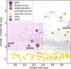 |
Fig. 1. F200W − F356W color vs. F356W magnitude distribution of JWST-detected sources in the J1030 field. The gray dots represent the extended sources, while point-like sources are shown as yellow filled circles. Stars align along a horizontal sequence at F200W − F356W ∼ −0.9. Faint (F356W > 24) and red (F200W − F356W > 0) point-like objects (filled circles with red contour) are mostly LRD candidates at z > 4 (e.g., ID4879 at z = 5.95; see text for details). The three bright (F356W < 23), point-like objects above the stellar sequence are two standard, X-ray detected broad line AGNs (J1030 and XID10, shown as filled circles with blue contours) and the BiRD (purple pentagon; see text for details). The dotted line shows the track followed by the BiRD if moved at different redshifts as labeled from z = 2 to z = 7. The smaller pentagons show for comparison the position of two spectroscopically confirmed LRDs at cosmic noon, discovered with JWST, namely the Rosetta Stone at z = 2.26 (plum; Juodžbalis et al. 2024a) and RUBIES-BLAGN-1 at z = 3.1 (pink; Wang et al. 2025). The colored box shows the selection region used to compute the space density of LRDs at cosmic noon (see Section 5.4). |
We inspected the three objects with F356W < 23 and F200W − F356W ∼ 0, as they appear redder than stars and brighter than LRDs. The brightest two are luminous, X-ray detected, broad line quasars: namely J1030 at z = 6.31 and XID10 at z = 2.74 (Marchesi et al. 2021), with F356W = 19.3 and 21.5, respectively. The third object, with F356W ∼ 22.4, is not detected in the X-rays, nor in the radio band (see Sect. 5.1), and was not previously identified spectroscopically. In Table 1 we present all the available photometry for this object, which was also previously detected in our ground-based photometry (Mignoli et al., in prep.), while in Fig. 2 we show the cutouts. The corresponding WFSS two-dimensional (2D) spectrum shows two emission lines superimposed on continuum emission (Fig. 3). Unfortunately, in the red part (λ > 3.8 μm) of the frame, a bright source contaminates the target’s spectrum. We optimally extracted the spectrum over 5 pixels and identified the two lines as the He Iλ 10 830 emission and Paschen γ (Paγ, hereafter), obtaining an initial redshift estimate of z ∼ 2.33. Once the redshift was estimated based on the two brightest lines in the spectrum, a faint emission line at 37 595 Å was also identified and attributed to the [O I] λ 11 290 line. We named the source BiRD (‘big red dot’) because it stands out in the NIRCam images when compared to the other, much fainter, LRD candidates at higher redshifts in the field.
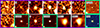 |
Fig. 2. Multiwavelength cutouts of BiRD. The images (5′′ × 5′′ each) were obtained with CTIO (B; MUSYC survey; Gawiser et al. 2006), LBT/LBC (g, r, i, z), CFHT/WIRCAM (Y, J, K), JWST/NIRCam (F115W, F200W, F356W), and Spitzer/IRAC (CH1 and CH2; Annunziatella et al. 2018). The JWST images are enclosed in green squares. The RGB image includes the NIRCam filters only. |
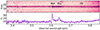 |
Fig. 3. 2D and 1D spectrum of BiRD (NIRCam/WFSS). The dotted box indicates the five-pixel aperture used to extract the 1D spectrum. We see clear emission from He I, Paγ, and O I lines, superimposed on the continuum. The contamination from a bright source is visible at the red end of the spectrum. The flux density Fλ is expressed in units of 10−16 erg s−1 cm−2 μm−1. The 1σ error spectrum is reported as a purple shaded area. |
Photometry of the BiRD.
4. Analysis
4.1. Spectral line fitting
We fit the BiRD spectrum using a Markov chain Monte Carlo (MCMC) method with the Python package emcee (Foreman-Mackey et al. 2013). We used a linear continuum and four Gaussian components to reproduce the line emission. We modeled both He I and Paγ using a narrow and a broad component. We tied the narrow components to have the same redshift, which we assumed to be the systemic one, and the same width, as we expect that they are both emitted from the narrow line region (NLR). We applied an absorption term to the broad He I line and to the continuum emission to account for a clear absorption feature at 3.6 μm (see Fig. 4). Starting from Eq. (9.2) of Draine (2011), we modeled the observed, attenuated flux I(λ) of these two components in the wavelength space as
 (1)
(1)
 |
Fig. 4. Continuum and line fit of BiRD. The NIRCam/WFSS spectrum is shown in purple with the corresponding errors (shaded area). We modeled both the He I (pink) and the Paγ (violet) emission with a narrow and a broad Gaussian component. An absorption term was applied to both continuum emission and broad He I line to account for the feature at 3.60 μm. We show the fit residuals in the bottom panel (lilac). |
where I0(λ) is the intrinsic, unabsorbed continuum or the He I unattenuated broad line flux and τ(λ) is the optical depth near line center. The latter is parametrized as (see Draine 2011, Eq. (9.7)):
 (2)
(2)
where τ0 is the optical depth at the line center, λ0 is the absorber central wavelength, σv is the velocity dispersion and c the speed of light (both in km s−1). Here, we are assuming that the absorber affects the radiation from the accretion disk and the broad line region (BLR); namely, it is located in the BLR or just outside it, to compare our results with other works (see, e.g., D’Eugenio et al. 2025; Inayoshi & Maiolino 2025; Ji et al. 2025; Juodžbalis et al. 2024a). However, we note that based on our data only, the absorber location is unconstrained. Thus, we took into consideration a different location for the absorber (discussed in Sect. 5.3). In particular, we investigated how additionally applying the absorption term to the narrow He I component would affect the column density of the absorber.
We used uniform priors for all parameters. For the narrow and broad components, we allowed the line width to be less than 1000 and 10 000 km s−1, respectively. We estimated the best values as the median of 10 000 realizations and the errors as the 16th and 84th percentiles. We derived the quantities presented in Table 2 from the fitted parameters, while the fit is shown in Fig. 4. For the absorber, we report the derived quantities in Table 3 (see Sect. 5.3 for the column density). We took into account the instrumental broadening by subtracting in quadrature the instrumental FWHM, which is  at our wavelengths, from the FWHM of the fitted lines. The correction was applied only to the narrow components and for the absorber, as it is irrelevant for the broad components.
Quantities derived from the line fit.
Properties of the absorber.
From the narrow components, we estimated a systemic redshift of  . The velocity shifts of the broad He I and Paγ are essentially unconstrained by our fit, while the FWHM of both lines exceed 2000 km s−1 . The absorber is blueshifted by
  km s−1 compared to the He I narrow component (see Table 3). The fitted quantities are independent of the adopted assumptions. We checked that by performing a free fit (i.e., without any tied parameters) or tying in the line width and centroid of the broad components as well, we would indeed obtain values that are consistent (within the errors) with the quantities reported in Tables 2 and 3.
4.2. SED analysis
With the source redshift in hand, we inspected its rest-frame broadband SED by combining the JWST photometry with optical, UV, and NIR photometry from the ground (the BiRD falls outside the region covered by HST/ACS and WFC3 observations), and with Spitzer NIR and mid-IR photometry. For the derivation of ground-based magnitudes and IRAC-CH1 and -CH2 magnitudes (3.6 and 4.5 μm, respectively), we refer to Mignoli et al. (in prep., see also Morselli et al. 2014; Annunziatella et al. 2018). As for the IRAC-CH3 and -CH4 magnitudes (5.8 and 8.0 μm, respectively) and the MIPS 24 μm magnitude, we downloaded the available mosaics from the Spitzer Enhanced Imaging Products (SEIP) archive3 and performed photometric measurements based on an updated version of the PhoEBO pipeline (Gentile et al. 2024). This pipeline uses high-resolution Ks-band images to define prior positions and shapes of sources, which are then used to separate blended objects in the lower-resolution IRAC-CH3, IRAC-CH4, and MIPS 24 μm bands. The priors were extracted with the Python implementation of Source Extractor (Barbary 2016). To model how these sources would appear in the lower-resolution images, we convolved the priors with matching kernels built from the PSFs of each band, and the model best-fit fluxes were derived by minimizing the residuals over the observed data (see Gentile et al. 2024). The BiRD is not detected in the IRAC-CH3, IRAC-CH4 and MIPS 24 μm maps. The corresponding 3σ limiting magnitudes are reported in Table 1.
As shown in Fig. 5, the rest-frame broadband SED of the BiRD shows an inflection point close to the 3645 Å Balmer break, reminiscent of the v-shaped SED of LRDs. We fitted power-law spectra of the form fλ ∝ λβ to the photometric data-points blueward and redward of the Balmer break, and determined the UV and optical rest spectral slopes, respectively. We found βUV, rest = −0.80 ± 0.16 for the UV slope. For the optical slope, we found βopt, rest = 2.74 ± 0.23 when limiting the fit to the data-points below 7000 Å rest-frame (i.e., where the SED peaks). Since Hα emission can contaminate photometric measurements around this peak, at 2 μm in the observed frame, we also performed a fit conservatively ignoring the JWST F200W and the WIRCAM K-band photometry, and just used the JWST F115W and F356W photometry, finding βopt, rest = 0.22 ± 0.16. We note that this second approach is very conservative since, based on what is observed for Rosetta Stone (Juodžbalis et al. 2024a), removing Hα emission would not be expected to reduce the observed K-band flux by more than ∼30%. Either way, our measured slopes satisfy the selection criteria of βUV, rest < −0.37 and βopt, rest > 0 adopted by Kocevski et al. (2025) to select LRDs at all redshifts. Therefore, the BiRD stands out as a spectroscopically confirmed LRD at cosmic noon.
 |
Fig. 5. Broadband, rest-frame SED of BiRD (purple symbols) compared to that of the Rosetta Stone (plum; Juodžbalis et al. 2024a), RUBIES-BLAGN-1 (pink; Wang et al. 2025) and to the median SED of LRDs at 3 ≲ z ≲ 9 (red; Casey et al. 2024). The green contour highlights the JWST data-points at 1.15, 2.0, and 3.56 μm, while the inverted triangles represent flux upper limits. The photometric errors for BiRD are also reported and, for some data-points, are smaller than the symbol size. The position of the Balmer break is marked by the vertical line at 3645 Å. |
In Fig. 5, we also compare the rest-frame SED of the BiRD with that of Rosetta Stone at z = 2.26 (Juodžbalis et al. 2024a) and RUBIES-BLAGN-1 (Wang et al. 2025) at z = 3.1, and with the median rest-frame SED of 675 LRDs at all redshifts derived by Casey et al. (2024). Except for a downturn above ∼1 μm rest-frame, the BiRD has a very similar SED to the Rosetta Stone and RUBIES-BLAGN-1. In addition, because of their relatively low redshift, they are a factor of 10–30 brighter than the average population of LRDs.
5. Results
5.1. Bolometric luminosity and X-ray and radio properties
Most spectroscopically identified LRDs display broad Balmer lines in their spectra, which are commonly used to estimate their bolometric luminosity and black hole mass, assuming standard scaling relations for quasars (see Sect. 5.2). In particular, the extinction-corrected luminosity of the broad Hα component can be converted into bolometric AGN luminosity using the relation of Stern & Laor (2012), expressed as
 (3)
(3)
In the absence of direct spectroscopic coverage at ∼6500 Å rest-frame, we estimated the luminosity of the broad Hα line starting from the broad Paγ component and assuming Case B in the theory of recombination-line radiation. This gives LHα, broad = 31.7 × LPaγ, broad ∼ 2.6 × 1043 erg s−1, and, in turn, Lbol ∼ 3 × 1045 erg s−1 (1.2 − 7.0 × 1045 erg s−1 when accounting for the dispersion in the Stern & Laor 2012 relation). We note that even if Case B might not always apply in the high-density AGN BLR (Ilić et al. 2012), it seems to work well for the Rosetta Stone: as a matter of fact, the luminosity of the broad Paγ line measured in the Rosetta Stone aligns very well with the expectations of case B recombination once the luminosities of its broad Hα and Hβ lines are corrected for extinction using the observed Balmer decrement. We discuss further implications of adopting case B recombination in Sect. 6.2.
Based on the estimated bolometric luminosity, we verified whether the BiRD, similarly to most LRDs, is severely underluminous in the X-rays compared to standard AGNs. The BiRD is not detected in the deep, 500 ks Chandra exposure of the J1030 field (Nanni et al. 2020; Marchesi et al. 2021). It is located at 3.25 arcmin from the exposure-weighted aimpoint of the Chandra mosaic, where the 90% encircled energy radius is 1.5″ at 1.5 keV and 2.5″ at 6.4 keV. To estimate approximate 3σ upper limits to source counts, we considered background counts extracted within annuli of inner radii 1.5″, 2.0″ and 2.5″, for the 0.5–7 keV (full, FB), 0.5–2 keV (soft, SB), 2–7 keV (hard, HB) band, respectively, and outer radii of 10″ for all X-ray bands, and then computed the binomial no-source probability (Weisskopf et al. 2007; Vito et al. 2019; Nanni et al. 2020). We obtained ∼3σ limits of 5, 3, and 6 counts in the FB, SB, and HB, respectively, that we then converted into limits to the source count rates after correcting for the assumed aperture and for the small loss of effective area at the BiRD’s position. Finally, assuming a standard power-law spectrum with a photon index of Γ = 1.9 (Peca et al. 2021; Signorini et al. 2023) and no intrinsic absorption, we obtained 3σ upper limits of 1.7 × 10⁻¹⁶, 7.1 × 10⁻¹⁷, 3.3 × 10⁻¹⁶ erg cm−2 s−1 to the source flux in the FB, SB, and HB, respectively. The soft band flux returns the most stringent constraint to the 2–10 keV rest-frame luminosity of L2 − 10 keV, rest < 3.7 × 1042 erg s−1. This, in turn, implies a bolometric correction of Lbol/L2 − 10 keV, rest > 800, which is at least 30 times larger than the average expected value for standard AGNs (see Fig. 6) and therefore calls for either very heavy suppression or intrinsically weak X-ray emission (Maiolino et al. 2025).
 |
Fig. 6. X-ray (2–10 keV) bolometric correction vs. bolometric luminosity for the standard population of broad line quasars (slate blue filled circles; Lusso et al. 2020) and the new population of X-ray silent, broad line AGNs discovered by JWST at z > 4 (Maiolino et al. 2025). The latter is shown with red triangles, which represent lower limits to the bolometric correction. The cyan area shows the relation found by Duras et al. (2020) for broad line AGNs with its dispersion. Similarly to the new JWST population, the BiRD is undetected in the X-rays (purple triangle), and its X-ray bolometric correction is at least 30 times larger than expected in standard quasars. The lower limits to the bolometric correction for the Rosetta Stone (in plum) and RUBIES-BLAGN-1 (pink triangle) are also shown for comparison. |
The BiRD is also undetected in the deep radio image of the J1030 field, which reaches a rms of 2.5 μJy at 1.4 GHz (D’Amato et al. 2022). The BiRD falls in the region of maximum radio sensitivity, and its non-detection corresponds to a 3σ limit to the rest frame 1.4 GHz luminosity of L1.4 GHz < 3 × 1039 erg s−1, assuming a standard spectral slope of α = −0.7 (with Sν ∝ να). We estimated the expected radio luminosity of BiRD assuming that it is a standard AGN and using literature calibrations (Panessa et al. 2019, 2015; D’Amato et al. 2022). We considered the correlation between intrinsic 2–10 keV and 1.4 GHz luminosity found by D’Amato et al. (2022) for non-jetted (radio-quiet) AGNs. We derived the intrinsic expected 2–10 keV X-ray luminosity from the bolometric one using the correlation from Duras et al. (2020), obtaining L1.4 GHz, exp = 6.7 × 1039 erg s−1. This would increase to L1.4 GHz, exp = 1040 erg s−1 if instead the intrinsic X-ray luminosity was computed using the LHα − L2 − 10 keV, rest relation from Jin et al. (2012). The radio luminosity of the BiRD is therefore at least 0.3 − 0.5 dex lower than expected on the basis of average correlations for standard AGNs. However, because of the systematics and scatter in the adopted relations, deeper radio data would be needed to confirm this difference and assess its significance.
5.2. Black hole mass
We derive the black hole mass of BiRD using two independent approaches, which both start from the Paγ broad line. In the first one, we use Eq. (2) from Landt et al. (2013), which employs the Paγ FWHM and the 1 μm rest-frame continuum to estimate the black hole mass
![Mathematical equation: $$ \begin{aligned} \log \left( \frac{M_{\rm BH}}{\mathrm{M_{\odot }} }\right) = 0.88 \left[2 \log \left(\frac{FWHM(\mathrm {Pa} \gamma )}{\mathrm{km\, s^{-1}}}\right) + 0.5 \log \left( \frac{\nu L_{1\,\upmu \mathrm{m}}}{\mathrm{erg\, s^{-1}}} \right) \right] -17.39. \end{aligned} $$](/articles/aa/full_html/2025/11/aa55946-25/aa55946-25-eq23.gif) (4)
(4)
We use the FWHM of the broad Paγ component determined in our fit. Unfortunately, the 1 μm rest-frame continuum is outside the range of our spectrum. However, we note that the fitted continuum appears to be flat (Fig. 4 and Fig. 3); therefore, we used the continuum underlying Paγ (i.e., 1.09 μm rest-frame) as a surrogate. Using Eq. (4), we obtained a black hole mass of

While the formal error on the BH mass of the estimate above is around the 30%, we note that the calibration of Landt et al. (2013) is characterized by an intrinsic scatter of ∼1 dex.
An alternative approach to derive the black hole mass is based on using the Paγ broad component to infer the properties of the Hα broad line. The latter is more often used as a black hole mass tracer in low-redshift active galaxies. Using the relation of Reines & Volonteri (2015), we can estimate the black hole mass as
 (5)
(5)
Adopting a different calibration, i.e., Greene & Ho (2005), systematically lowers the black hole masses by a factor of ∼2.
We based our argument on the analogy between BiRD and Rosetta Stone. As previously mentioned (see Sect. 5.1), the hypothesis of case B recombination seems to work well for the Rosetta Stone. The broad Paγ in the Rosetta Stone appears not to be significantly dust-attenuated, as the observed broad line ratio of Paγ and Paβ is ∼0.525, very close to the intrinsic one (∼0.55; Osterbrock 1989). Thus, based on the intrinsic Hα and Paγ flux ratio ∼31.7 (Osterbrock 1989), we can infer the unextincted Hα broad line luminosity ∼7 × 1043 erg s−1 from the observed broad Paγ line in the Rosetta Stone. Substituting in Eq. (5), we find for the Rosetta Stone a black hole mass  . This estimate is nicely consistent with the value obtained from the measured Hα luminosity, corrected for dust extinction based on the observed Hα /Hβ broad line ratio, i.e., log(MBH/M⊙) = 8.67 ± 0.30, which becomes log(MBH/M⊙) = 8.47 ± 0.30, if the extinction correction is based on the narrow lines (Juodžbalis et al. 2024a).
We thus apply the same argument to BiRD. The inferred broad Hα luminosity from the observed Paγ is in this case  .
.
Another ingredient that goes in Eq. (5) to estimate the black hole mass is the FWHM of the Hα line. We note that in the Rosetta Stone the ratio between the FWHM of broad Hα and Paγ lines is ∼1.57. We assume that the same ratio holds for BiRD. On the other hand, Wang et al. (2025) found a lower ratio FWHM(Hα)/FWHM(Paγ)∼1.43 in RUBIES-BLAGN-1. We account for this difference when computing the errors on the black hole mass. By applying Eq. (5), we find

We note that the calibration of Reines & Volonteri (2015) has an intrinsic scatter ∼0.5 dex. This estimate of the black hole mass of BiRD is fully consistent with the value that we obtained adopting the relation of Landt et al. (2013), taking into account the 1 dex scatter of the latter relation. Using the calibration of Greene & Ho (2005) would result in a decrease of the black hole mass by a factor of ∼2, reducing the difference between the two estimates. In the discussion in Sect. 6.5, where we report the active black hole mass function (BHMF) of LRDs, we include the black hole mass  of the BiRD derived from Hα using the calibration of Reines & Volonteri (2015) to ease comparisons with other works.
5.3. He I absorption
We estimated the column density of He I atoms that generate the absorption in the BiRD spectrum (Fig. 4). As seen in Sect. 4.1, we start considering a scenario in which the absorber acts on both the continuum radiation and the BLR (see also Juodžbalis et al. 2024a). The absorption of the bound-bound transition 23S − 23P of He I depends on the number density along the line of sight (column density). The column density N(He I) can be estimated using the apparent optical depth method (Savage & Sembach 1991). Given N(v), the column density per unit velocity, we integrated Eq. (8) of Savage & Sembach (1991) and solved for N = ∫N(v)dv,
![Mathematical equation: $$ \begin{aligned} N(\mathrm{He\ I}) = \int N(v) dv = 3.768 \times 10^{14} (f\lambda _{\rm rest})^{-1} \int \tau (v) dv\ [\mathrm {cm}^{-2}] ,\end{aligned} $$](/articles/aa/full_html/2025/11/aa55946-25/aa55946-25-eq30.gif) (6)
(6)
where f and λrest are the oscillator strength and the rest-frame wavelength of the He I line expressed in Å (10 830 Å), respectively, and τ(v) is the optical depth as a function of velocity. We consider the oscillator strength for the 23P to 23S transition from Drake (2006), f = 0.5390861 (see their Table 11.11). We integrated Eq. (6) to obtain

which corresponds to the column density of He I atoms in the 23S level. We note that the absorption is blueshifted by  km s−1 (see Table 3). This suggests that the absorber is outflowing from the nuclear region.
We also evaluated how a different location of the absorber would affect the derived He I column density. As we discuss in Sect. 4.1, our data cannot constrain the location of the absorber and it is thus necessary to consider other scenarios. We repeated the fit (see Sect. 4.1) by applying the absorption term also to the narrow He I component; namely, by assuming that the absorber is located outside of the NLR (see also Wang et al. 2025, who considered a similar hypothesis). In this case, we obtained a lower value of the column density,  . This difference is expected as the absorber is now acting on the entire emitted flux (from the continuum, BLR and NLR) and, thus, it has a lower optical depth. Also, in this case, the absorption is blueshifted, with
  km s−1 , meaning that the gas is outflowing. We note that the absorber location does not affect the blueshifted velocity, which is consistent within the errors in the two different assumptions.
5.4. Space density of LRDs at cosmic noon
The discovery of the BiRD adds to that of the Rosetta Stone and RUBIES-BLAGN-1, leading us to attempt a first measurement of the space density of LRDs around cosmic noon based on JWST data. The BiRD has been selected as a bright outlier in the color–magnitude diagram of point-like sources in the J1030 field (see Fig. 1), as it was both falling above the stellar sequence and sufficiently distant from the locus occupied by fainter, high-z LRDs. The selection box can be described as follows: F200W − F356W > −0.4, F356W < 23.0. Both the Rosetta Stone and RUBIES-BLAGN1 satisfy these selection criteria (Fig. 1).
Based on the observed SED of the BiRD, we estimated the color–magnitude track that an LRD would follow when moved at different redshifts: for z < zmin ∼ 2, LRDs would mix with stars and would not be selected by their F200W − F356W color. Also, in addition to the applied limiting magnitude (F356W < 23) to select relatively luminous objects, we applied another color cut at F200W − F356W < 2 to consider only LRDs at z ≲ 3.5 (see Fig. 1). This redshift limit is also consistent with the SEDs of the other two LRDs.
Since we are dealing with objects that are well above the flux limit of the survey fields in which they were discovered, we used the simple 1/Vmax method (Schmidt 1968) to estimate their number density,
 (7)
(7)
where ΔlogL is the width of the luminosity bin, wi are weights that account for incompleteness effects, and Vmax, i is the maximum volume in which an object i would have been detected, i.e.,
 (8)
(8)
where dVc/dz is the comoving volume element and fΩ is the fraction of the solid angle of the sky covered by the observations. The confidence intervals in Φ(L) were computed following the standard approximations of Gehrels (1986) for low count statistics.
We adopted zmin = 2.0 and zmax = 3.5 for all three objects. The correspondence between the adopted color selection criteria and the effective redshift boundaries clearly depends on the chosen SED track, but we note that statistical uncertainties greatly exceed those produced by the choice of the exact redshift limits.
Rather, an important source of uncertainty is related to the completeness of our sample. The J1030 (EIGER), JADES, and RUBIES survey fields are covered by deep JWST imaging of comparable depth, and any of the three considered objects would have been detected in any of the considered survey fields. However, other sources in the JADES and RUBIES fields might satisfy our selection criteria; hence, we have wi ≥ 1 for both Rosetta Stone and RUBIES-BLAGN-1. In our estimate, we conservatively assumed wi = 1 and treated our measurement of the space density of z ∼ 2.5 LRDs as a lower limit.
We considered a total solid angle of Ωtot = ΩJ1030 + ΩJADES + ΩRUBIES = 302 arcmin2 with ΩJ1030, ΩJADES, ΩRUBIES = 27, 125, and 150 arcmin2, respectively, corresponding to fΩ = 2.03 × 10⁻⁶. To compute Φ(L), we considered the bolometric luminosities of the three objects derived from their broad Balmer or Paschen lines and used a luminosity bin of 0.5 dex as it spans the full luminosity range covered by the three targets (3, 3.9, 9.3 × 1045 erg s−1 for the BiRD, RUBIES-BLAGN-1, and the Rosetta Stone, respectively). This gives  Mpc−3 dex−1 at Lbol, mean = 5.4 × 1045 erg s−1 and zmean ∼ 2.5 (see Fig. 7).
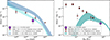 |
Fig. 7. Left: space density of LRDs at Lbol, mean = 5.4 × 1045 erg s−1 and zmean ∼ 2.5 from our work (purple pentagon) compared with the bolometric luminosity function derived at similar redshifts for the entire AGN population (steel blue; Shen et al. 2020) and for blue, UV-selected, unobscured AGNs (pale turquoise; Kulkarni et al. 2019). The shaded areas correspond to the 16th and 84th percentiles of the bolometric LFs. At cosmic noon, the measured abundance of LRDs appears to be a factor 2 − 3 lower than that of unobscured AGNs. We also compare our estimate with the bolometric luminosity function of LRDs at 4.5 < z < 6.5 from Kokorev et al. (2024) (in red). Right: space density of LRDs at zmean ∼ 2.5 and MBH ∼ 6.3 × 10⁸ M⊙ (purple) compared with the predicted active BHMF from broad line quasars at similar redshift (dark cyan; Shen & Kelly 2012) and the active BHMF of LRDs at higher redshifts (red symbols, Matthee et al. 2024; Taylor et al. 2025). The shaded area corresponds to the 16th and 84th percentiles of the model active BHMF value. |
Admittedly, the centering of the 0.5-dex luminosity bin has been chosen to include all three sources, and is therefore arbitrary. If a random positioning of 0.5-dex-wide bins was adopted, the three sources would split into two adjacent bins, returning, on average, space densities that are about two times lower than the measured value. Given the very small source statistics, all measurements would be nonetheless consistent with each other within the errors, and therefore we adopt the quoted value of  Mpc−3 dex−1 as our reference measurement.
6. Discussion
6.1. The absorber
In Sect. 5.3, we describe how we estimated the column density of He I that produces the observed absorption in the BiRD spectrum. As mentioned before, we note that based on our data we cannot constrain the location of the absorber. Juodžbalis et al. (2024a) also find in the Rosetta Stone blueshifted absorption feature in the He I line profile (Δv = −506 ± 7 km s−1 and FWHM = 714 ± 14 km s−1), and in the broad Balmer lines. Due to its resonant nature, the He I transition is much easier to see in absorption compared to Balmer lines, which require higher gas and column densities.
For Rosetta Stone, two scenarios are discussed here: the first one considering a single absorber producing both absorptions and the second considering two separate absorbers, with the highest density one being responsible for Balmer absorption. In both scenarios, based on CLOUDY modeling, they estimate the hydrogen density  , which favors a BLR origin for the Balmer absorbing clouds. Assuming the same origin also for the He I absorbing clouds, Juodžbalis et al. (2024a) find in the Rosetta Stone a He I column density in the 23S level of
  . A BLR origin for the absorbing gas was adopted also by D’Eugenio et al. (2025), Inayoshi & Maiolino (2025), Ji et al. (2025). In the same scenario, we derive for BiRD
  , which is a factor of ∼3 lower than the value seen in the Rosetta Stone.
Blueshifted He I absorption was also found by Wang et al. (2025) in RUBIES-BLAGN-1. The absorption is blueshifted by  km s−1 and a FWHM of 569 ± 23 km s−1 . The blueshift seen in RUBIES-BLAGN-1 is very similar to that observed in BiRD (
 km s−1), while our FWHM is lower (
 km s−1). Regarding the column density, Wang et al. (2025) assumes that the absorber acts on the entire emitted radiation (continuum, BLR and NLR). They find a He I column density N(He I)=(5.9 ± 0.3)×1013 cm−2. This value is consistent with the value that we find for the BiRD under the same hypothesis, i.e., in the case of an absorber located outside of the NLR (
 ).
).
Similar He I absorption was previously detected in active galaxies and quasars at low redshift (Hutchings et al. 2002; Landt et al. 2019; Pan et al. 2019). Several works about JWST-discovered broad line AGNs report Balmer absorption, with a detection rate that is much higher compared to low-redshift AGNs (Juodžbalis et al. 2024a; Kocevski et al. 2025; Lin et al. 2024; Maiolino et al. 2024; Matthee et al. 2024). Unfortunately, due to the limited wavelength coverage of our data, we cannot verify if Balmer absorptions also affect the spectrum of BiRD, and we cannot estimate the hydrogen density.
The similarity in the He I absorption displayed by BiRD, Rosetta Stone, and RUBIES-BLAGN-1 suggests that this feature could be common among LRDs at cosmic noon. Thus, observing the He I line in more objects at z ∼ 2 − 3 will be crucial for a better understanding of the properties of the absorbing gas. In principle, it is possible that the He I absorption also affects the spectra of high-redshift (z > 4) LRDs, as it has been seen for Balmer absorption. Unfortunately, this feature can be seen with NIRSpec gratings and NIRCam grisms only up to z ≲ 4, which might explain why the detections were reported only at z ∼ 2 − 3.
6.2. SED shape, dust content, and optical extinction
As shown in Fig. 5, the SED of the BiRD is very similar to that of the Rosetta Stone and of RUBIES-BLAGN-1, as well as to the median SED of LRDs at higher redshifts (Casey et al. 2024), at least below 1 μm rest-frame. Above that wavelength, the BiRD SED has a marked downturn that is not observed in the typical SED of LRDs. Since the BiRD is detected only up λrest ∼ 1.3 μm (IRAC-CH2), it is unclear whether and how strongly this downturn would continue at longer wavelengths. In any case, the current upper limits at ∼1.7 − 6.3 μm in the rest frame already indicate that the BiRD’s emission at those wavelengths cannot be as strong as that of the Rosetta Stone or RUBIES-BLAGN-1.
In RUBIES-BLAGN-1, the relatively flat – or even declining – SED (in terms of λfλ) at rest-frame wavelengths λ > 1 μm has been interpreted by Wang et al. (2025) as evidence of the absence of emission from hot dust at temperatures around 1000 − 1500 K. This hot dust, typically located in the parsec-scale circumnuclear torus, is usually responsible for the rising AGN SED at λrest > 1 μm (Richards et al. 2006; Trefoloni et al. 2025). The downturn observed in the BiRD SED above that wavelength would argue even more strongly against the presence of a hot dusty torus.
In general, however, observations of LRDs mid-IR SEDs do not rule out the presence of circumnuclear dusty tori with different physical or geometrical properties, such as clumpy tori where the self-shielding of individual clouds leads to colder mean temperatures (Nenkova et al. 2008), or tori with dust grain composition skewed toward large grains and extended on tens of pc scales (Li et al. 2025). In any case, the average SED of LRDs points toward an overall low dust content in these systems.
Based on the compact sizes of the sources and assuming that dust reddening is responsible for the observed SED shape just above the Balmer break, Casey et al. (2024) estimated an average dust mass in high-z LRDs of Md ∝  Nd ∼ 104 M⊙, where Rd and Nd are the effective radius and column density of the dust distribution, respectively, and Nd ∝ AV. Such dust-poor systems are significantly rare at any epoch. In the nearby Universe they are confined to a handful of extremely metal-poor blue-compact dwarfs (Fisher et al. 2014; Calura 2025). At earlier times the census is even sparser: recent ALMA studies reveal only a few high-redshift galaxies with similarly weak dust emission, implying gas-to-dust ratios ∼300 − 1000 (e.g., Spilker et al. 2025). However, the limitation of the approach of Casey et al. (2025) is that the average dust column density is measured along the line of sight, which is sensitive to the geometric distribution of dust and is likely biased toward low column densities.
In any case, even if the estimated dust masses were to be regarded as lower limits, all the observational evidence points toward a low content of dust at any temperature in LRDs. All the attempts to detect the millimeter and submillimeter (mm/submm) continuum in these systems using ALMA – including RUBIES-BLAGN-1 (Akins et al. 2025; Setton et al. 2025) – have been unsuccessful, placing upper limits on the total dust mass at temperatures of a few tens of K of Md ≲ 108 M⊙ from individual observations, and of Md ≲ 107 M⊙ from a stacked sample of 60 LRDs (Casey et al. 2025).
Dust extinction in LRDs is generally measured through SED fitting, assuming that the observed red continuum results from dust attenuation of an intrinsically blue spectrum produced by stars or an AGN. By using this technique, Kokorev et al. (2024) report for dust extinction an average AV = 1.6 in their sample, while Akins et al. (2024) find values that can be ≳3 mag in several objects. The differences in the AV values are possibly due to different selections of LRDs. High AV values hardly reconcile with the results on individual objects reported by Chen et al. (2025), who find upper limits to the optical extinction values of AV ≲ 1.0 − 1.5 mag by modeling the dust reprocessing with various extinction curves and incident spectra.
An alternative way to derive AV is via Balmer decrement. Assuming case B recombination and using the ratio of narrow lines, the values of AV are in the range of AV ∼ 0.5 − 1.4 for individual LRDs as RUBIES-BLAGN-14 (Wang et al. 2025), the Rosetta Stone (Juodžbalis et al. 2024a), and BlackTHUNDER (D’Eugenio et al. 2025). Using broad lines increases these values to AV ≲ 2.3 − 3.15.
Based on the reasoning above, we caution that incorrectly high AV values from Balmer lines, possibly due to deviations from case B recombination, could lead to an overestimate of the intrinsic Hα luminosity. Thus, this could also lead to a corresponding overestimation in the inferred bolometric luminosity and black hole mass.
6.3. X-ray weakness, obscuration, and black hole accretion
As reported in Section 5.1, the BiRD is not detected in the deep Chandra image of the field. This places an upper limit to its 2 − 10 keV rest-frame luminosity of L2 − 10 keV, rest < 3.7 × 1042 erg s−1, which is at least 30 times lower than what would be expected for a standard broad line AGN of equal bolometric luminosity (Duras et al. 2020; see Fig. 6). Similarly to what has been observed in high-z LRDs and in the BLAGN population discovered by JWST, the BiRD is therefore surprisingly weak in the X-rays, and the reasons for this widespread X-ray weakness in LRDs are still under scrutiny.
If the BiRD had standard, type-1 AGN bolometric corrections, to depress its intrinsic 2 − 10 keV luminosity by a factor of ∼30, absorption by gas column densities of at least 1024 cm−2, that is Compton-thick, is needed (Gilli et al. 2007; Lanzuisi et al. 2018)6. Heavy, Compton-thick absorption by dust-poor or dust-free gas such as that in the BLR clouds or their immediate surroundings has indeed been proposed to explain the widespread X-ray weakness of LRDs (Maiolino et al. 2025), provided that the BLR covering factor is significantly larger than in standard AGNs. The large equivalent width of the broad Hα line commonly observed in JWST BLAGNs, as well as the frequent presence of an absorption component in the Balmer lines and of a prominent Balmer break in those systems featuring high-quality spectra, could corroborate this interpretation (Maiolino et al. 2025; Juodžbalis et al. 2025).
In addition to heavy nuclear absorption, it is often hypothesized that JWST BLAGNs are X-ray weak because they accrete at super-Eddington rates (Madau & Haardt 2024; Pacucci & Narayan 2024; King 2025; Madau 2025). At high accretion rates, geometrically thick disks could form around black holes, leading to a highly anisotropic emission. At large viewing angles from the polar axis, the innermost, hottest regions of the accretion flow (inner disk and corona) are shadowed by the outer cooler regions of the thick disk, leading to a significant luminosity decrease, especially in the X-rays (Madau 2025).
Furthermore, in the above geometry, the UV photon density is such to Compton-cool the electrons in the corona much more efficiently than in standard thin disk plus corona models, making the emerging X-ray spectrum very soft (Γ ∼ 3 − 4; Pacucci & Narayan 2024; Madau & Haardt 2024). These two effects lead these models to predict 2 − 10 keV bolometric corrections of k2 − 10 keV > 100 − 1000 (Madau & Haardt 2024; Pacucci & Narayan 2024), similar to what is observed. However, we note that the average Eddington ratio measured for JWST BLAGNs is λE ∼ 0.1 (Juodžbalis et al. 2025) and the X-ray weakness persists also for “dormant” AGNs discovered by JWST at high-z, accreting at only 1% of the Eddington limit (Juodžbalis et al. 2024b), suggesting that super-Eddington accretion might not be the only explanation for the X-ray weakness for the whole population.
When accounting for the large uncertainties in its estimated bolometric luminosity and black hole mass, we infer for the BiRD an Eddington ratio of  . Similar values are measured for both the Rosetta Stone and RUBIES-BLAGN-1. In the thick-disk super-Eddington model by Madau (2025), such low values of the apparent Eddington ratio can be obtained only at inclinations larger than 80 deg, meaning that most JWST AGNs should be observed almost edge-on. This can hardly be reconciled with random disk orientations: at 57 degrees – the average viewing angle for random disk inclinations – one would expect in this model λE ∼ 3.
However, in other studies of super-Eddington accretion flows, the decrease of the apparent luminosity with the thick disk inclination is much more rapid, owing to the very narrow opening the funnel formed by the accretion flow (Ohsuga et al. 2005), and this tension might be alleviated. We also note that super-Eddington accretion might still be tenable if the BH masses were overestimated by one or two orders of magnitude. This has been in fact proposed by recent works suggesting that either Balmer scattering (Naidu et al. 2025) or electron scattering (Rusakov et al. 2025) from a layer of very dense and ionized gas around the BLR might broaden the Balmer lines far above their kinematic width.
While these scenarios are intriguing, they await confirmation as they seem in contrast with the finding that the same profiles are seen in local AGNs, whose BH masses area measured directly, and might even be in contrast with some features observed in the Paschen and Balmer lines of JWST BLAGNs (see Juodžbalis et al. 2025 for a full discussion). Moreover, for obscured AGN candidates at z ∼ 6 in the SHELLQs survey (Matsuoka et al. 2025), which exhibit narrow Lyα lines and broad Hα components that are significantly weaker than their narrow counterparts compared to local quasars, it has recently been suggested that the BLR is partially hidden (Iwasawa et al. 2025). If this is the case also for LRDs, then their BH masses might have been instead underestimated, making these objects even more puzzling.
6.4. Space density and evolution of LRDs
In Fig. 7 (left panel) we compare our measured space density of LRDs at z ∼ 2.5 with the bolometric luminosity function of all AGNs (Shen et al. 2020) and UV-selected QSOs (Kulkarni et al. 2019) at similar redshifts. Shen et al. (2020) considered AGN samples selected at different wavelengths, from the IR to the X-rays and, based on a detailed SED modeling, derived bolometric and extinction corrections for all objects in their samples. Their measurements are therefore supposed to include both populations of obscured and unobscured AGNs, providing an estimate of the bolometric luminosity function of the whole AGN population and of its evolution up to z ∼ 7. Based on a large sample of quasars selected by their blue UV/optical colors, Kulkarni et al. (2019) estimated the luminosity function at 1450 Å rest-frame of unobscured AGNs up to z ∼ 7.5. To convert their measurements from UV to bolometric AGN luminosities, we used a bolometric correction of Lbol/L1450 = 4.0, consistent e.g., with the estimates of Richards et al. (2006) and Runnoe et al. (2012).
As shown in Fig. 7, the density of LRDs at z ∼ 2.5 is only a factor of ∼2 − 3 lower than that of standard UV-selected quasars with similar bolometric luminosity, and consistent with it within the errors. As already mentioned in Sect. 5.4, the measured abundance of LRDs could even be treated as a lower limit. In fact, other LRDs at z ∼ 2 − 3 awaiting for spectroscopic confirmation might be present in the JADES and/or RUBIES fields, each covering a factor of ∼5 larger area than the EIGER observation of J1030.
However, we caution that it remains unclear whether the presence of similar objects has already been ruled out in other JWST fields, which would instead bias our measurement to higher values. As the analysis of JWST data in well-studied survey fields progresses, the number of spectroscopically confirmed LRDs at z ∼ 2 − 3 is steadily increasing (Hviding et al. 2025; Zhuang et al. 2025). We therefore consider it reasonable to assume that LRDs at z ∼ 2 − 3 in other JWST deep survey fields have yet to be discovered, primarily because of the current incompleteness of the spectroscopic analysis and follow-up. Therefore, we find the three fields analyzed in this study offer a representative sampling of the LRD population at these redshifts.
To date, the vast majority of LRDs, including those confirmed spectroscopically, have been discovered at z > 4. Their abundance in those epochs has been found to largely exceed that of standard AGNs, even by up to one order of magnitude (Kocevski et al. 2025). However, a fair comparison between the luminosity function of LRDs and standard AGNs is complicated by the still unknown physical properties of the former, which makes any estimate of their intrinsic bolometric luminosity highly uncertain. For example, it is unclear whether their observed rest-UV luminosities can be reliably used to infer their intrinsic bolometric luminosities. The measured rest-UV luminosities of LRDs are in fact significantly lower than the expected intrinsic value derived by fitting their optical/NIR SEDs with standard AGN templates and once correcting for extinction, yet higher (by up to two dex) than what the best fit extinction would produce (Kokorev et al. 2024; Matthee et al. 2024). The same uncertainties apply to the UV luminosity function recently derived for the LRD candidates at all redshifts selected through Euclid photometry (Euclid Collaboration 2025).
Here we consider Hα emission as a more reliable proxy of the LRD bolometric luminosity, as it is less prone to extinction effects than UV emission and it is directly related to the total, intrinsic UV photon production. However, we note that at high neutral hydrogen column densities, such as those proposed by Inayoshi & Maiolino (2025) for LRDs, a fraction of the Hα photons can be absorbed by electrons in the n = 2 energy level. This would depress the observed Hα line luminosity, thus further increasing the uncertainty related to the bolometric luminosity and black hole mass of LRDs from the observed Hα .
Our measurement of the bolometric luminosity function of LRDs at z ∼ 2.5 can be compared with that measured by Kokorev et al. (2024) at z > 4 (which, however, is derived from the SED fitting of candidate LRDs with photometric redshift only). At Lbol = 5.4 × 1045 erg s−1, the abundance of LRDs increases from z ∼ 2.5 to z = 5.5 by a factor of 4. At z = 5.5 their abundance is 5x larger than that of standard, pre-JWST AGNs of comparable bolometric luminosity (Shen et al. 2020; not shown in Fig. 7), whereas it rapidly falls below it by a factor of ∼7 at z ∼ 2.5 (see Fig. 7).
Despite this rapid decline as the Universe ages, the abundance of LRDs at cosmic noon remains significant, as also possibly confirmed by the results of Ma et al. (2025), who leveraged ground-based photometric selection of LRDs over a ∼3 deg2 area and derived optical luminosity functions at z ∼ 2 − 3. When correcting the observed 5500 Å luminosities in Ma et al. (2025) using an extinction of AV ∼ 1.6, i.e. the average value quoted by Kokorev et al. (2024) for their sample, and assuming a bolometric correction of 10 (Richards et al. 2006), their measurements convert into a space density of z ∼ 2 − 3 LRDs with Lbol ∼ 5 × 1045 erg s−1 equal to ∼3 × 10⁻⁶ Mpc−3 dex−1, which is very similar to our result.
This large abundance of LRDs at cosmic noon is particularly remarkable if compared with the expectations from recent models, which suggest LRDs might be able to probe the very first and rapid growth of BH seeds (Inayoshi 2025). According to these models, BH seeds of mass 104 − 5 M⊙ might grow via super-Eddington accretion in dense environments, and be able to reach masses of 107 − 8 M⊙ in less than 10 Myr. After this early, rapid growth phase, because of the reduced mass supply from its close environment, the AGN transitions from super-Eddington to more typical accretion.
Inayoshi (2025) demonstrated that the abundance of LRDs at z > 5 and the abundance of AGNs at z < 5 can be reproduced by a model of stochastic BH accretion, in which the first one or two accretion episodes correspond to the LRD phase. In this model, the abundance of LRDs at z ∼ 2.5 is expected to fall short of that of standard AGNs by three dex. This is in line with the expectations of other theoretical arguments that suggest that the formation rate of seed BHs is strongly suppressed at z < 5. This is expected to happen as metals diffuse throughout the intergalactic medium favoring cloud cooling and fragmentation, and, in turn, preventing the direct collapse of large gas clouds into massive seed BHs (Bellovary et al. 2011).
However, at z ∼ 2.5, we found that the abundance of LRDs is at most a factor of 7 lower than that of standard AGNs. This might serve as an indication that the formation of BH seeds does not halt at z < 5 and that it remains somewhat efficient to at least cosmic noon.
6.5. Active black hole mass function
We study the space density of LRDs at zmean ∼ 2.5 as a function of the black hole mass. We use the black hole masses inferred from the Hα line using the relation of Reines & Volonteri (2015). Wang et al. (2025) adopt in their work the calibration of Greene & Ho (2005) to compute the Hα – based black hole mass of RUBIES-BLAGN-1. We thus multiply their estimate by a factor of 2 to account for the systematic difference between the two relations.
The black hole masses of the three LRDs span over a mass bin of 1 dex centered at  , and thus we have to divide the space density at Lbol, mean by a factor 2, as it was computed for a bin size of 0.5 dex (Φ(MBH)∼2 × 10⁻⁶ Mpc−3dex−1). Besides the bin size, we do not expect that other effects impact the space density at MBH, mean. However, we note that, because of the color-magnitude selection box defined in Sect. 5.4, and based on the rough correlation between F356W magnitude and BH mass observed in the few known LRDs at z = 2.0 − 3.5 (Juodžbalis et al. 2024a; Wang et al. 2025; Ma et al. 2025; Zhuang et al. 2025), we expect to sample high (MBH ≳ 108 M⊙) black hole masses.
In Fig. 7 (right panel) we compare the space density of LRDs at zmean ∼ 2.5 and  with the model BHMF of accreting BHs inferred from SDSS broad line QSOs at similar redshift (z = 2.65; Shen & Kelly 2012). For
  and z = 2.65 the SDSS data are indeed incomplete; therefore, we made comparison with the predicted7 active BHMF of BLQSOs based on the observations. We see that our estimate is only a factor ≲2 below the expectation for BLQSOs and consistent within the errors, thus implying that LRDs contribute in a way that is similar to BLQSOs to the population of black holes with a similar mass at z ∼ 2.5.
We also compare our estimate with the active BHMF derived for JWST-discovered BLAGNs at higher redshifts (Matthee et al. 2024; Taylor et al. 2025). We note that also in these works the black hole masses are computed using the calibration by Reines & Volonteri (2015), so we do not apply any scaling factor to their active BHMFs. On the other hand, both Matthee et al. (2024) and Taylor et al. (2025) do not correct the Hα luminosity for dust attenuation when estimating the black hole masses. Compared to the last bins of Matthee et al. (2024) and Taylor et al. (2025), which partially overlap with our 1 dex-mass bin, we find that our estimate is a factor ∼3.8 − 4.4 lower but consistent within the errors.
We note that Matthee et al. (2024) and Taylor et al. (2025) select their objects looking for broad-line emitters. Therefore, their active BHMFs include objects that are not LRDs. The fraction of LRDs is about 1/3 of the sample from Taylor et al. (2025). This means that their estimates would decrease when considering the BLAGNs that are also LRDs. For the work by Taylor et al. (2025), we evaluate a decrement of the active BHMF by a factor of less than 2 in the last mass bin, due to the fact that the fraction of LRDs is higher than 1/3 in that bin, which thus would made their estimates closer to ours. Overall, bearing in mind the different selections, this comparison points in the direction of a mild evolution only in the abundance of LRDs from high redshift to cosmic noon.
7. Summary and conclusions
In this work, we report the study of BiRD, an LRD discovered at z ∼ 2.33 in the J1030 field, using JWST/NIRCam data (both imaging and slitless spectroscopy). This source has interesting analogies with two other LRDs at cosmic noon, namely, GN-28074 at z = 2.26 (Rosetta Stone, Juodžbalis et al. 2024a) and RUBIES-BLAGN-1 at z = 3.1 (Wang et al. 2025). The main conclusions of our work are given below.
-
Using the NIRCam/WFSS spectrum, we derived some physical properties of BiRD. The black hole mass, estimated with two independent methods starting from the broad Paγ emission, is on the order of ∼108 M⊙. We detected blueshifted He I absorpion (
 km s−1). A similar blueshifted feature is seen in the Rosetta Stone and in RUBIES-BLAGN-1. Depending on the absorber location, the He I column density is N(He I)∼0.5 − 1.2 × 1014 cm−2.
 -
Based on our study of the X-ray and radio properties of BiRD, we find the source is both radio and X-ray silent, with L1.4 GHz < 3 × 1039 erg s−1 and
 . Based on the bolometric luminosity
  , we determined a lower limit for the X-ray bolometric correction
  , consistent with the values of other JWST-discovered BLAGNs.
 -
We estimated the space density of LRDs at cosmic noon as a function of the bolometric luminosity Lbol and the black hole mass MBH. This is the first space density at that cosmic age that is constrained via spectroscopic data. We find
 Mpc−3 dex−1 at Lbol, mean = 5.4 × 1045 erg s−1 and zmean ∼ 2.5. This value is only a factor ∼2 − 3 lower than the value from UV-selected quasars at similar redshifts.
 -
Similarly, we find that for
 , the space density
  is a factor of ∼2 only below the expectation for broad line QSOs in the same cosmic epoch. In comparison with JWST-discovered BLAGNs at z ∼ 4.8, our estimate is a factor of ∼3.8 − 4.4 below the active BHMF of LRDs with similar black hole masses, but consistent within the errors.
Overall, our results point to only a mild evolution in the abundance of LRDs with decreasing redshift. Their space density remains significant at cosmic noon, comparable to that of BLQSOs.
In the future, we plan to further investigate the properties of BiRD using multiwavelength data. According to Maiolino et al. (2025), the X-ray weakness of LRDs might be explained by dense, dust-poor or dust-free gas in BLR clouds. Future JWST/NIRSpec observations of the rest-frame optical spectrum of BiRD, with particular attention paid to the Balmer break and Balmer absorptions, would allow us to test whether this scenario also applies in this system. Regarding the dust properties, follow-up observations of BiRD in the mid-IR and millimeter regimes with JWST/MIRI and ALMA, respectively, are essential to placing robust constraints on the amounts of hot and cold dust in this system. MIRI observations will also allow us to detect the He I + Paγ lines in other LRDs at higher redshifts and verify if He I absorptions are widespread in BLAGNs also before the cosmic noon. Another interesting development of our study would be to extend the search for objects similar to BiRD using larger areas of the sky. This will enable the sampling of a wider luminosity-and-black hole mass space for the computation of the luminosity function and BHMF of LRDs at cosmic noon. All the future expansions of this work are pivotal in shedding more light on the elusive nature of LRDs.
For RUBIES-BLAGN-1, we estimate AV from the Hα and Paγ flux reported in Table 4 of Wang et al. (2025), assuming an unextincted Paγ flux and using either the Small Magellanic Cloud (Gordon et al. 2003) or Calzetti (Calzetti et al. 2000) extinction law for both narrow and broad lines.
We note that D’Eugenio et al. (2025) assume for broad lines an intrinsic Hα /Hβ ratio of 3.1 (Dong et al. 2008), which is different from case B. However, this assumption does not significantly impact the value of AV.
This estimate assumes absorption by gas with solar abundances. Sub-solar abundances, often observed in the ISM of JWST high-z galaxies and AGNs (Curti et al. 2024), would lead to even larger densities.
We note that the turnover at the low-mass end in Fig. 7 (right panel) might suffer from the poor sampling of low-mass BHs in the SDSS sample (Shen & Kelly 2012).
Acknowledgments
We thank the referee for their useful and constructive comments. We thank Guido Risaliti for useful discussion and for kindly providing us with the data-points of Fig. 6. We acknowledge support from the INAF 2022/2023 “Ricerca Fondamentale” grants. K.I. acknowledges support under the grant PID2022-136827NB-C44 provided by MCIN/AEI/10.13039/501100011033 / FEDER, UE. I.J. and R.M. acknowledges support by the Science and Technology Facilities Council (STFC), by the ERC through Advanced Grant 695671 “QUENCH”, and by the UKRI Frontier Research grant RISEandFALL. I.J. acknowledges support also by the Huo Family Foundation through a P.C. Ho PhD Studentship. R.M. also acknowledges funding from a research professorship from the Royal Society. M.S. acknowledges financial support from the Italian Ministry for University and Research, through the grant PNRR-M4C2- I1.1-PRIN 2022-PE9-SEAWIND: Super-Eddington Accretion: Wind, INflow and Disk-F53D23001250006-NextGenerationEU. This work is based on observations made with the NASA/ESA/CSA James Webb Space Telescope. The data were obtained from the Mikulski Archive for Space Telescopes at the Space Telescope Science Institute, which is operated by the Association of Universities for Research in Astronomy, Inc., under NASA contract NAS 5-03127 for JWST. These observations are associated with the GTO program 1243.
References
- Akins, H. B., Casey, C. M., Allen, N., et al. 2023, ApJ, 956, 61 [NASA ADS] [CrossRef] [Google Scholar]
- Akins, H. B., Casey, C. M., Lambrides, E., et al. 2024, ArXiv e-prints [arXiv:2406.10341] [Google Scholar]
- Akins, H. B., Casey, C. M., Chisholm, J., et al. 2025, ArXiv e-prints [arXiv:2503.00998] [Google Scholar]
- Ananna, T. T., Bogdán, Á., Kovács, O. E., Natarajan, P., & Hickox, R. C. 2024, ApJ, 969, L18 [NASA ADS] [CrossRef] [Google Scholar]
- Annunziatella, M., Marchesini, D., Stefanon, M., et al. 2018, PASP, 130, 124501 [NASA ADS] [CrossRef] [Google Scholar]
- Barbary, K. 2016, J. Open Source Softw., 1, 58 [Google Scholar]
- Barro, G., Pérez-González, P. G., Kocevski, D. D., et al. 2024, ApJ, 963, 128 [CrossRef] [Google Scholar]
- Bellovary, J., Volonteri, M., Governato, F., et al. 2011, ApJ, 742, 13 [Google Scholar]
- Bertin, E., & Arnouts, S. 1996, A&AS, 117, 393 [NASA ADS] [CrossRef] [EDP Sciences] [Google Scholar]
- Bushouse, H., Eisenhamer, J., Dencheva, N., et al. 2025, JWST Calibration Pipeline [Google Scholar]
- Calura, F. 2025, ArXiv e-prints [arXiv:2506.13851] [Google Scholar]
- Calzetti, D., Armus, L., Bohlin, R. C., et al. 2000, ApJ, 533, 682 [NASA ADS] [CrossRef] [Google Scholar]
- Casey, C. M., Akins, H. B., Kokorev, V., et al. 2024, ApJ, 975, L4 [Google Scholar]
- Casey, C. M., Akins, H. B., Finkelstein, S. L., et al. 2025, ArXiv e-prints [arXiv:2505.18873] [Google Scholar]
- Chen, K., Li, Z., Inayoshi, K., & Ho, L. C. 2025, ArXiv e-prints [arXiv:2505.22600] [Google Scholar]
- Curti, M., Maiolino, R., Curtis-Lake, E., et al. 2024, A&A, 684, A75 [NASA ADS] [CrossRef] [EDP Sciences] [Google Scholar]
- D’Amato, Q., Gilli, R., Vignali, C., et al. 2020, A&A, 636, A37 [NASA ADS] [CrossRef] [EDP Sciences] [Google Scholar]
- D’Amato, Q., Prandoni, I., Gilli, R., et al. 2022, A&A, 668, A133 [NASA ADS] [CrossRef] [EDP Sciences] [Google Scholar]
- de Graaff, A., Brammer, G., Weibel, A., et al. 2025a, A&A, 697, A189 [NASA ADS] [CrossRef] [EDP Sciences] [Google Scholar]
- de Graaff, A., Rix, H. W., Naidu, R. P., et al. 2025b, A&A, 701, A168 [NASA ADS] [CrossRef] [EDP Sciences] [Google Scholar]
- Delvecchio, I., Gruppioni, C., Pozzi, F., et al. 2014, MNRAS, 439, 2736 [NASA ADS] [CrossRef] [Google Scholar]
- D’Eugenio, F., Maiolino, R., Perna, M., et al. 2025, ArXiv e-prints [arXiv:2503.11752] [Google Scholar]
- Dong, X., Wang, T., Wang, J., et al. 2008, MNRAS, 383, 581 [NASA ADS] [Google Scholar]
- Draine, B. T. 2011, Physics of the Interstellar and Intergalactic Medium, ed. P. U. Press [Google Scholar]
- Drake, G. 2006, in Springer Handbook of Atomic, ed. G. W. F. Drake, 199 [Google Scholar]
- Duras, F., Bongiorno, A., Ricci, F., et al. 2020, A&A, 636, A73 [NASA ADS] [CrossRef] [EDP Sciences] [Google Scholar]
- Euclid Collaboration (Bisigello, L., et al.) 2025, https://doi.org/10.1051/0004-6361/202554537 [Google Scholar]
- Fisher, D. B., Bolatto, A. D., Herrera-Camus, R., et al. 2014, Nature, 505, 186 [NASA ADS] [CrossRef] [Google Scholar]
- Foreman-Mackey, D., Hogg, D. W., Lang, D., & Goodman, J. 2013, PASP, 125, 306 [Google Scholar]
- Fujimoto, S., Brammer, G. B., Watson, D., et al. 2022, Nature, 604, 261 [NASA ADS] [CrossRef] [Google Scholar]
- Gardner, J. P., Mather, J. C., Abbott, R., et al. 2023, PASP, 135, 068001 [NASA ADS] [CrossRef] [Google Scholar]
- Gawiser, E., van Dokkum, P. G., Herrera, D., et al. 2006, ApJS, 162, 1 [CrossRef] [Google Scholar]
- Gehrels, N. 1986, ApJ, 303, 336 [Google Scholar]
- Gentile, F., Talia, M., Behiri, M., et al. 2024, ApJ, 962, 26 [NASA ADS] [CrossRef] [Google Scholar]
- Gilli, R., Comastri, A., & Hasinger, G. 2007, A&A, 463, 79 [NASA ADS] [CrossRef] [EDP Sciences] [Google Scholar]
- Gordon, K. D., Clayton, G. C., Misselt, K. A., Landolt, A. U., & Wolff, M. J. 2003, ApJ, 594, 279 [NASA ADS] [CrossRef] [Google Scholar]
- Greene, J. E., & Ho, L. C. 2005, ApJ, 630, 122 [NASA ADS] [CrossRef] [Google Scholar]
- Greene, J. E., Labbe, I., Goulding, A. D., et al. 2024, ApJ, 964, 39 [CrossRef] [Google Scholar]
- Hainline, K. N., Maiolino, R., Juodžbalis, I., et al. 2025, ApJ, 979, 138 [Google Scholar]
- Harikane, Y., Zhang, Y., Nakajima, K., et al. 2023, ApJ, 959, 39 [NASA ADS] [CrossRef] [Google Scholar]
- Hutchings, J. B., Crenshaw, D. M., Kraemer, S. B., et al. 2002, AJ, 124, 2543 [NASA ADS] [CrossRef] [Google Scholar]
- Hviding, R. E., de Graaff, A., Miller, T. B., et al. 2025, A&A, 702, A57 [NASA ADS] [CrossRef] [EDP Sciences] [Google Scholar]
- Ilić, D., Popović, L. Č., La Mura, G., Ciroi, S., & Rafanelli, P. 2012, A&A, 543, A142 [NASA ADS] [CrossRef] [EDP Sciences] [Google Scholar]
- Inayoshi, K. 2025, ApJ, 988, L22 [Google Scholar]
- Inayoshi, K., & Maiolino, R. 2025, ApJ, 980, L27 [Google Scholar]
- Iwasawa, K., Gilli, R., Vito, F., et al. 2025, ArXiv e-prints [arXiv:2505.04826] [Google Scholar]
- Ji, X., Maiolino, R., Übler, H., et al. 2025, ArXiv e-prints [arXiv:2501.13082] [Google Scholar]
- Jin, C., Ward, M., & Done, C. 2012, MNRAS, 425, 907 [NASA ADS] [CrossRef] [Google Scholar]
- Juodžbalis, I., Ji, X., Maiolino, R., et al. 2024a, MNRAS, 535, 853 [CrossRef] [Google Scholar]
- Juodžbalis, I., Maiolino, R., Baker, W. M., et al. 2024b, Nature, 636, 594 [CrossRef] [Google Scholar]
- Juodžbalis, I., Maiolino, R., Baker, W. M., et al. 2025, ArXiv e-prints [arXiv:2504.03551] [Google Scholar]
- Kashino, D., Lilly, S. J., Matthee, J., et al. 2023, ApJ, 950, 66 [CrossRef] [Google Scholar]
- King, A. 2025, MNRAS, 536, L1 [Google Scholar]
- Kocevski, D. D., Finkelstein, S. L., Barro, G., et al. 2025, ApJ, 986, 126 [Google Scholar]
- Kokorev, V., Caputi, K. I., Greene, J. E., et al. 2024, ApJ, 968, 38 [NASA ADS] [CrossRef] [Google Scholar]
- Kulkarni, G., Worseck, G., & Hennawi, J. F. 2019, MNRAS, 488, 1035 [Google Scholar]
- Labbe, I., Greene, J. E., Matthee, J., et al. 2024, ArXiv e-prints [arXiv:2412.04557] [Google Scholar]
- Labbe, I., Greene, J. E., Bezanson, R., et al. 2025, ApJ, 978, 92 [NASA ADS] [CrossRef] [Google Scholar]
- Landt, H., Ward, M. J., Peterson, B. M., et al. 2013, MNRAS, 432, 113 [NASA ADS] [CrossRef] [Google Scholar]
- Landt, H., Ward, M. J., Kynoch, D., et al. 2019, MNRAS, 489, 1572 [NASA ADS] [CrossRef] [Google Scholar]
- Lanzuisi, G., Civano, F., Marchesi, S., et al. 2018, MNRAS, 480, 2578 [Google Scholar]
- Li, Z., Inayoshi, K., Chen, K., Ichikawa, K., & Ho, L. C. 2025, ApJ, 980, 36 [Google Scholar]
- Lin, X., Wang, F., Fan, X., et al. 2024, ApJ, 974, 147 [NASA ADS] [CrossRef] [Google Scholar]
- Lusso, E., Risaliti, G., Nardini, E., et al. 2020, A&A, 642, A150 [NASA ADS] [CrossRef] [EDP Sciences] [Google Scholar]
- Ma, Y., Goulding, A., Greene, J. E., et al. 2024, ApJ, 974, 225 [NASA ADS] [CrossRef] [Google Scholar]
- Ma, Y., Greene, J. E., Setton, D. J., et al. 2025, ArXiv e-prints [arXiv:2504.08032] [Google Scholar]
- Madau, P. 2025, ArXiv e-prints [arXiv:2501.09854] [Google Scholar]
- Madau, P., & Dickinson, M. 2014, ARA&A, 52, 415 [Google Scholar]
- Madau, P., & Haardt, F. 2024, ApJ, 976, L24 [Google Scholar]
- Maiolino, R., Scholtz, J., Curtis-Lake, E., et al. 2024, A&A, 691, A145 [NASA ADS] [CrossRef] [EDP Sciences] [Google Scholar]
- Maiolino, R., Risaliti, G., Signorini, M., et al. 2025, MNRAS, 538, 1921 [Google Scholar]
- Marchesi, S., Mignoli, M., Gilli, R., et al. 2021, A&A, 656, A117 [NASA ADS] [CrossRef] [EDP Sciences] [Google Scholar]
- Matsuoka, Y., Onoue, M., Iwasawa, K., et al. 2025, ApJ, 988, 57 [Google Scholar]
- Matthee, J., Naidu, R. P., Brammer, G., et al. 2024, ApJ, 963, 129 [NASA ADS] [CrossRef] [Google Scholar]
- Mazzolari, G., Gilli, R., Maiolino, R., et al. 2024, ArXiv e-prints [arXiv:2412.04224] [Google Scholar]
- Mazzolari, G., Scholtz, J., Maiolino, R., et al. 2025, A&A, 700, A12 [NASA ADS] [CrossRef] [EDP Sciences] [Google Scholar]
- Mignoli, M., Gilli, R., Decarli, R., et al. 2020, A&A, 642, L1 [EDP Sciences] [Google Scholar]
- Morselli, L., Mignoli, M., Gilli, R., et al. 2014, A&A, 568, A1 [NASA ADS] [CrossRef] [EDP Sciences] [Google Scholar]
- Naidu, R. P., Matthee, J., Katz, H., et al. 2025, ArXiv e-prints [arXiv:2503.16596] [Google Scholar]
- Nanni, R., Gilli, R., Vignali, C., et al. 2020, A&A, 637, A52 [NASA ADS] [CrossRef] [EDP Sciences] [Google Scholar]
- Nenkova, M., Sirocky, M. M., Ivezić, Ž., & Elitzur, M. 2008, ApJ, 685, 147 [Google Scholar]
- Ohsuga, K., Mori, M., Nakamoto, T., & Mineshige, S. 2005, ApJ, 628, 368 [NASA ADS] [CrossRef] [Google Scholar]
- Onoue, M., Inayoshi, K., Ding, X., et al. 2023, ApJ, 942, L17 [NASA ADS] [CrossRef] [Google Scholar]
- Osterbrock, D. E. 1989, Astrophysics of Gaseous Nebulae and Active Galactic Nuclei (University Science Books) [Google Scholar]
- Pacucci, F., & Narayan, R. 2024, ApJ, 976, 96 [NASA ADS] [CrossRef] [Google Scholar]
- Pan, X., Zhou, H., Liu, W., et al. 2019, ApJ, 883, 173 [NASA ADS] [CrossRef] [Google Scholar]
- Panessa, F., Tarchi, A., Castangia, P., et al. 2015, MNRAS, 447, 1289 [NASA ADS] [CrossRef] [Google Scholar]
- Panessa, F., Baldi, R. D., Laor, A., et al. 2019, Nat. Astron., 3, 387 [Google Scholar]
- Peca, A., Vignali, C., Gilli, R., et al. 2021, ApJ, 906, 90 [Google Scholar]
- Pérez-González, P. G., Barro, G., Rieke, G. H., et al. 2024, ApJ, 968, 4 [CrossRef] [Google Scholar]
- Reines, A. E., & Volonteri, M. 2015, ApJ, 813, 82 [NASA ADS] [CrossRef] [Google Scholar]
- Richards, G. T., Strauss, M. A., Fan, X., et al. 2006, AJ, 131, 2766 [Google Scholar]
- Rinaldi, P., Rieke, G. H., Wu, Z., et al. 2025, ArXiv e-prints [arXiv:2507.17738] [Google Scholar]
- Runnoe, J. C., Brotherton, M. S., & Shang, Z. 2012, MNRAS, 422, 478 [Google Scholar]
- Rusakov, V., Watson, D., Nikopoulos, G. P., et al. 2025, ArXiv e-prints [arXiv:2503.16595] [Google Scholar]
- Savage, B. D., & Sembach, K. R. 1991, ApJ, 379, 245 [NASA ADS] [CrossRef] [Google Scholar]
- Schmidt, M. 1968, ApJ, 151, 393 [Google Scholar]
- Setton, D. J., Greene, J. E., Spilker, J. S., et al. 2025, ArXiv e-prints [arXiv:2503.02059] [Google Scholar]
- Shen, X., Hopkins, P. F., Faucher-Giguère, C.-A., et al. 2020, MNRAS, 495, 3252 [Google Scholar]
- Shen, Y., & Kelly, B. C. 2012, ApJ, 746, 169 [NASA ADS] [CrossRef] [Google Scholar]
- Signorini, M., Marchesi, S., Gilli, R., et al. 2023, A&A, 676, A49 [NASA ADS] [CrossRef] [EDP Sciences] [Google Scholar]
- Spilker, J. S., Whitaker, K. E., Narayanan, D., et al. 2025, ArXiv e-prints [arXiv:2507.16914] [Google Scholar]
- Stepney, M., Banerji, M., Tang, S., et al. 2024, MNRAS, 533, 2948 [CrossRef] [Google Scholar]
- Stern, J., & Laor, A. 2012, MNRAS, 423, 600 [NASA ADS] [CrossRef] [Google Scholar]
- Stiavelli, M., Djorgovski, S. G., Pavlovsky, C., et al. 2005, ApJ, 622, L1 [NASA ADS] [CrossRef] [Google Scholar]
- Sun, F., Egami, E., Pirzkal, N., et al. 2023, ApJ, 953, 53 [NASA ADS] [CrossRef] [Google Scholar]
- Taylor, A. J., Finkelstein, S. L., Kocevski, D. D., et al. 2025, ApJ, 986, 165 [Google Scholar]
- Trefoloni, B., Gilli, R., Lusso, E., et al. 2025, A&A, 697, A223 [NASA ADS] [CrossRef] [EDP Sciences] [Google Scholar]
- Übler, H., Maiolino, R., Curtis-Lake, E., et al. 2023, A&A, 677, A145 [NASA ADS] [CrossRef] [EDP Sciences] [Google Scholar]
- Vito, F., Brandt, W. N., Yang, G., et al. 2018, MNRAS, 473, 2378 [Google Scholar]
- Vito, F., Brandt, W. N., Bauer, F. E., et al. 2019, A&A, 630, A118 [NASA ADS] [CrossRef] [EDP Sciences] [Google Scholar]
- Wang, B., de Graaff, A., Davies, R. L., et al. 2025, ApJ, 984, 121 [Google Scholar]
- Weisskopf, M. C., Wu, K., Trimble, V., et al. 2007, ApJ, 657, 1026 [Google Scholar]
- Yue, M., Eilers, A.-C., Ananna, T. T., et al. 2024, ApJ, 974, L26 [CrossRef] [Google Scholar]
- Zeballos, M., Aretxaga, I., Hughes, D. H., et al. 2018, MNRAS, 479, 4577 [Google Scholar]
- Zhuang, M. Y., Li, J., Shen, Y., et al. 2025, ArXiv e-prints [arXiv:2505.20393] [Google Scholar]
All Tables
All Figures
|
Fig. 1. F200W − F356W color vs. F356W magnitude distribution of JWST-detected sources in the J1030 field. The gray dots represent the extended sources, while point-like sources are shown as yellow filled circles. Stars align along a horizontal sequence at F200W − F356W ∼ −0.9. Faint (F356W > 24) and red (F200W − F356W > 0) point-like objects (filled circles with red contour) are mostly LRD candidates at z > 4 (e.g., ID4879 at z = 5.95; see text for details). The three bright (F356W < 23), point-like objects above the stellar sequence are two standard, X-ray detected broad line AGNs (J1030 and XID10, shown as filled circles with blue contours) and the BiRD (purple pentagon; see text for details). The dotted line shows the track followed by the BiRD if moved at different redshifts as labeled from z = 2 to z = 7. The smaller pentagons show for comparison the position of two spectroscopically confirmed LRDs at cosmic noon, discovered with JWST, namely the Rosetta Stone at z = 2.26 (plum; Juodžbalis et al. 2024a) and RUBIES-BLAGN-1 at z = 3.1 (pink; Wang et al. 2025). The colored box shows the selection region used to compute the space density of LRDs at cosmic noon (see Section 5.4). |
| In the text | |
|
Fig. 2. Multiwavelength cutouts of BiRD. The images (5′′ × 5′′ each) were obtained with CTIO (B; MUSYC survey; Gawiser et al. 2006), LBT/LBC (g, r, i, z), CFHT/WIRCAM (Y, J, K), JWST/NIRCam (F115W, F200W, F356W), and Spitzer/IRAC (CH1 and CH2; Annunziatella et al. 2018). The JWST images are enclosed in green squares. The RGB image includes the NIRCam filters only. |
| In the text | |
|
Fig. 3. 2D and 1D spectrum of BiRD (NIRCam/WFSS). The dotted box indicates the five-pixel aperture used to extract the 1D spectrum. We see clear emission from He I, Paγ, and O I lines, superimposed on the continuum. The contamination from a bright source is visible at the red end of the spectrum. The flux density Fλ is expressed in units of 10−16 erg s−1 cm−2 μm−1. The 1σ error spectrum is reported as a purple shaded area. |
| In the text | |
|
Fig. 4. Continuum and line fit of BiRD. The NIRCam/WFSS spectrum is shown in purple with the corresponding errors (shaded area). We modeled both the He I (pink) and the Paγ (violet) emission with a narrow and a broad Gaussian component. An absorption term was applied to both continuum emission and broad He I line to account for the feature at 3.60 μm. We show the fit residuals in the bottom panel (lilac). |
| In the text | |
|
Fig. 5. Broadband, rest-frame SED of BiRD (purple symbols) compared to that of the Rosetta Stone (plum; Juodžbalis et al. 2024a), RUBIES-BLAGN-1 (pink; Wang et al. 2025) and to the median SED of LRDs at 3 ≲ z ≲ 9 (red; Casey et al. 2024). The green contour highlights the JWST data-points at 1.15, 2.0, and 3.56 μm, while the inverted triangles represent flux upper limits. The photometric errors for BiRD are also reported and, for some data-points, are smaller than the symbol size. The position of the Balmer break is marked by the vertical line at 3645 Å. |
| In the text | |
|
Fig. 6. X-ray (2–10 keV) bolometric correction vs. bolometric luminosity for the standard population of broad line quasars (slate blue filled circles; Lusso et al. 2020) and the new population of X-ray silent, broad line AGNs discovered by JWST at z > 4 (Maiolino et al. 2025). The latter is shown with red triangles, which represent lower limits to the bolometric correction. The cyan area shows the relation found by Duras et al. (2020) for broad line AGNs with its dispersion. Similarly to the new JWST population, the BiRD is undetected in the X-rays (purple triangle), and its X-ray bolometric correction is at least 30 times larger than expected in standard quasars. The lower limits to the bolometric correction for the Rosetta Stone (in plum) and RUBIES-BLAGN-1 (pink triangle) are also shown for comparison. |
| In the text | |
|
Fig. 7. Left: space density of LRDs at Lbol, mean = 5.4 × 1045 erg s−1 and zmean ∼ 2.5 from our work (purple pentagon) compared with the bolometric luminosity function derived at similar redshifts for the entire AGN population (steel blue; Shen et al. 2020) and for blue, UV-selected, unobscured AGNs (pale turquoise; Kulkarni et al. 2019). The shaded areas correspond to the 16th and 84th percentiles of the bolometric LFs. At cosmic noon, the measured abundance of LRDs appears to be a factor 2 − 3 lower than that of unobscured AGNs. We also compare our estimate with the bolometric luminosity function of LRDs at 4.5 < z < 6.5 from Kokorev et al. (2024) (in red). Right: space density of LRDs at zmean ∼ 2.5 and MBH ∼ 6.3 × 10⁸ M⊙ (purple) compared with the predicted active BHMF from broad line quasars at similar redshift (dark cyan; Shen & Kelly 2012) and the active BHMF of LRDs at higher redshifts (red symbols, Matthee et al. 2024; Taylor et al. 2025). The shaded area corresponds to the 16th and 84th percentiles of the model active BHMF value. |
| In the text | |
Current usage metrics show cumulative count of Article Views (full-text article views including HTML views, PDF and ePub downloads, according to the available data) and Abstracts Views on Vision4Press platform.
Data correspond to usage on the plateform after 2015. The current usage metrics is available 48-96 hours after online publication and is updated daily on week days.
Initial download of the metrics may take a while.