| Issue |
A&A
Volume 703, November 2025
|
|
|---|---|---|
| Article Number | A10 | |
| Number of page(s) | 10 | |
| Section | Cosmology (including clusters of galaxies) | |
| DOI | https://doi.org/10.1051/0004-6361/202556007 | |
| Published online | 31 October 2025 | |
Testing light-unaffiliated mass clumps in MACS 0416 on galaxy and galaxy-cluster scales using the JWST⋆
1
Aix Marseille Univ, CNRS, CNES, LAM, Marseille, France
2
School of Physics and Astronomy, University of Minnesota, Minneapolis, MN 55455, USA
3
Faculty of Mathematics and Physics, Jadranska ulica 19, SI-1000 Ljubljana, Slovenia
4
UHasselt – Flanders Make, Digital Future Lab, Wetenschapspark 2, B-3590 Diepenbeek, Belgium
⋆⋆ Corresponding author: This email address is being protected from spambots. You need JavaScript enabled to view it.
Received:
18
June
2025
Accepted:
20
August
2025
Abstract
Light-unaffiliated mass clumps (LUMCs), i.e. dark matter (DM) components without any stellar counterparts, have been reported in strong-lensing mass reconstructions of MACS 0416, both on galaxy and galaxy-cluster scales. On a galaxy-cluster scale, the most recent LENSTOOL parametric mass reconstruction based on 303 spectroscopically confirmed multiple images features a LUMC in the south of the cluster. On galaxy scale, the most recent GRALE non-parametric mass reconstruction based on 237 multiple images features two LUMCs, M1 and M2. Given the implications of these findings in the context of structure formation and evolution, we tested these features parametrically using the LENSTOOL code. First, we show that a mass model in which each large-scale DM component introduced in the modelling is associated with a stellar counterpart can reproduce the 303 multiple images, removing the need for any cluster-scale LUMC in MACS 0416. We then updated the GRALE non-parametric mass reconstruction using the 303 multiple images, finding that one of the two galaxy-scale LUMCs, M1, is no longer significant, while M2 remains. We tested M2 by explicitly including it in our parametric model, at the position and with the mass inferred from our updated GRALE model. We find that the inclusion of this LUMC does not improve the global root mean square (RMS), but mildly improves locally the RMS for one multiple image located close to M2. Besides, the preferred mass for M2 corresponds to the lowest mass allowed by the adopted prior. If we allow the mass of M2 to reach 0, then LENSTOOL converges to this null value, consistently rejecting M2. We present a detailed comparison of parametric and non-parametric models in the M2 area. It appears that both approaches show very similar surface mass density at this location, with a 5–6% difference between the mass maps. The difference is that GRALE favours a distinct mass substructure, while LENSTOOL favours a more diffuse mass distribution. We were able to propose a parametric mass model without including any LUMCs, providing further evidence of DM being associated with light in galaxy clusters. Finally, further investigations into the mass distribution at the M2 location are necessary. In this paper, we present two new mass models and associated products based on the 303 multiple images that will be hosted at the Strong Lensing Cluster Atlas Data Base at the Laboratoire d’Astrophysique de Marseille.
Key words: large-scale structure of Universe
Based on observations obtained with the James Webb Space Telescope (JWST).
© The Authors 2025
 Open Access article, published by EDP Sciences, under the terms of the Creative Commons Attribution License (https://creativecommons.org/licenses/by/4.0), which permits unrestricted use, distribution, and reproduction in any medium, provided the original work is properly cited.
This article is published in open access under the Subscribe to Open model. This email address is being protected from spambots. You need JavaScript enabled to view it. to support open access publication.
1. Introduction
Dark matter (DM) is an intriguing component that is thought to largely dominate the mass budget in astrophysical objects, in particular in galaxy clusters. The first indirect evidence for a ‘missing mass’ is almost 90 years old (Zwicky 1937), but we have no definitive statement about its existence and very limited clues with regard to its properties; we only have indirect evidence concerning DM. On the galaxy-cluster scale, both observations and numerical simulations do support the association between DM and light, that is, the associated stellar component, in most cases in the form of a bright galaxy. Observationally, no cluster scale DM clump without any associated light concentration has been reliably detected so far. In hydrodynamical simulations, stars do form in the potential well of DM halos (e.g. Borgani et al. 2004; Yoo et al. 2025).
However, parametric strong-lensing (SL) studies of galaxy clusters sometimes display ‘misleading features’ (see Limousin et al. 2022, for a discussion), in particular light-unaffiliated mass clumps (LUMCs); i.e. DM components without any stellar counterparts. The purpose of these LUMCs is usually to overcome the limitations of parametric methods; for example, to account for the complex morphology and elongation of the clusters, which sometimes cannot be properly captured by simple and idealised analytical formulae. Still, the interpretation of these LUMCs is not always properly mentioned or discussed by the authors, which might be misleading for the readers.
Recently, mass models featuring such LUMCs have been revisited in order to see if a DM traced by light (the stellar component) model can reproduce the multiple images. This was found to sometimes be the case, and sometimes not. Limousin et al. (2022, L22 hereafter) successfully revisited three parametric mass models featuring LUMCs, presenting models where dark matter is traced by light, with the goal of probing the inner shape of the DM density profile. More recently, Limousin et al. (2025) were unable to propose a mass model where DM is traced by light in the merging cluster Abell 370. In order to reach sub-arcsec precision in the adjustment of the multiple images, a cluster scale LUMC had to be introduced in the modelling, as also found in earlier works. Limousin et al. (2025) interpreted this finding as being symptomatic of the lack of realism of a parametric description of the DM distribution in such a complex merging cluster.
The association between DM clumps and light being central to this paper, we briefly discuss what ‘associated’ means to us. We refer to a ‘loose’ association: each DM clump has a well-identified stellar counterpart located at most a few dozen kiloparsec from it (which is what is allowed by a self-interacting DM scenario; see the discussion by L22), and the other properties are determined entirely by the lensed images, not the associated stellar component, which is usually a bright galaxy. A tight association would imply that DM clumps have the same centre, ellipticity, and position angle of the associated galaxy, and the mass and core radius would be related to that of the associated galaxy.
The galaxy cluster MACS 0416, which holds several records in terms of number of multiple images reported (Jauzac et al. 2014; Bergamini et al. 2023; Diego et al. 2024b; Rihtaršič et al. 2025), displays LUMCs, both on cluster (Bergamini et al. 2021, 2023; Rihtaršič et al. 2025) and galaxy scales (Perera et al. 2025b). In this paper, we aim to test if we can present a competitive mass model without the need for such LUMCs; i.e. where all (cluster- and galaxy-scale) DM components have a clear stellar counterpart. The light distribution in the core of MACS 0416 is trimodal (see green boxes in Fig. 1). There are two dominant Brightest Cluster Galaxies (BCGs), and a sub-dominant light concentration in the north-east. We used JWST data (F356W, F277W, and F115W filters) presented in Rihtaršič et al. (2025) to generate Fig. 1 and Fig. 2.
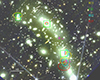 |
Fig. 1. Core of MACS 0416 from JWST data. North is up, east is left. We show the location of the cluster-scale DM clumps inferred in different studies by ellipses whose semi-axes are equal to the 3σ error bars on the position of these clumps: in yellow for Bergamini et al. (2021), in cyan for Bergamini et al. (2023), and in red for Rihtaršič et al. (2025). Green boxes represent the prior on the position of each cluster-scale DM clumps proposed by Limousin et al. (2022) and investigated in this work. In magenta, we show the location of the two galaxy-scale light-unaffiliated mass clumps inferred by Perera et al. (2025b). In white, we show the 303 secure multiple images reported by Rihtaršič et al. (2025). |
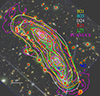 |
Fig. 2. Core of MACS 0416 from JWST data. We show the total convergence maps for all models: B21 in yellow; B23 in cyan; R25 in red; our updated GRALE model (PCANUCS) in magenta; and our updated LENSTOOL model (L25) in green. We also show the convergence map from Diego et al. (2024b) in white (D24). We show the location of M2 in blue. |
The number of halos constituting a given galaxy cluster is also important to investigate since the abundance of halos and sub-halos is a probe of the hierarchical structure formation scenario (e.g. Allen et al. 2011; Jauzac et al. 2015).
All our results use the Λ Cold Dark Matter (ΛCDM) concordance cosmology with ΩM = 0.3, ΩΛ = 0.7, and a Hubble constant of H0 = 70 km s−1 Mpc−1. At the redshift of MACS 0416 (z = 0.396), this cosmology implies a scale of 5.34 kpc/″.
2. LENSTOOL parametric-mass reconstructions
A number of parametric-mass reconstructions using LENSTOOL (Jullo et al. 2007) have been performed. Here, we only consider and discuss that performed since 2020, and we present a new one. They all use secure multiple images with known spectroscopic redshifts. They incorporate hot-gas mass distribution inferred from X-ray data. These models describe MACS 0416 as a superposition of cluster-scale and galaxy-scale DM halos, all described using a dPIE mass distribution (Limousin et al. 2005; Elíasdóttir et al. 2007). Galaxy-scale halos are associated with individual cluster members using the scaling laws described in these works in order to relate their mass with their luminosity. Importantly, these scaling laws were constrained using a prior which is based on the measure of the stellar velocity dispersion of cluster members (see Bergamini et al. 2021, 2023). Two galaxy-scales’ halos were optimised individually instead of using the scaling laws, since they were found to have an influence on some multiple images. Moreover, a number of cluster scale DM halos are introduced in the modelling. This is discussed in the following.
2.1. Pre-JWST data
Using Hubble Frontier Fields (HFF) and BUFFALO imaging data, complemented with ground-based spectroscopy (in particular MUSE), many secured multiply imaged systems were found in MACS 0416. Bergamini et al. (2021, B21 hereafter) reported 182 multiple images. They are reproduced by a four-DM-clumps model, whose positions are shown as yellow ellipses in Fig. 1. One of them, in the south, is not affiliated with light. This model reproduces the multiple images with an RMS of 0.40″. B21 also presented mass models that reproduce the 182 multiple images fairly well (RMS between 0.45″ and 0.48″ instead of 0.40″), where the DM is described using only three mass clumps. Based on three figures of merit (matching of the internal kinematics of the cluster members galaxies as well as BIC and AIC criteria), they selected the four-mass-clumps model as their reference.
L22 revisited this mass model by imposing that each cluster-scale DM halo must coincide with a luminous counterpart, imposing the position of each of the three DM halos to be within the green boxes shown on Fig. 1. They reproduced the 182 multiple images with an RMS of 0.49″.
Adding new MUSE spectroscopic data, Bergamini et al. (2023, B23 hereafter), reported 237 multiple images. They are reproduced with an RMS equal to 0.43″ by a four-DM-clumps model, whose positions are shown as cyan ellipses in Fig. 1. One of them, in the south, is not affiliated with light.
2.2. JWST data
Diego et al. (2024b) were the first to examine the JWST NIRCam imaging data from Prime Extragalactic Areas for Reionization and Lensing Science (PEARLS) survey, publishing a lens model along with a list of 343 multiple image candidates. Subsequently, Rihtaršič et al. (2025, R25 hereafter), identified additional candidates using NIRCam imaging from the CAnadian NIRISS Unbiased Cluster Survey (CANUCS) and obtained spectroscopic redshifts for a subset of the Diego et al. (2024b) and CANUCS candidates with JWST NIRSpec and NIRISS spectroscopy. This led to a final catalogue of 303 multiple images with spectroscopic confirmation, including most of the pre-JWST systems reported by B23, Richard et al. (2021), and Diego et al. (2024a). These images were reproduced with an RMS equal to 0.53″ by a four-DM-clumps model, whose positions are shown as red ellipses in Fig. 1. One of them, in the south, is not affiliated with light. Actually, neither B23 nor R25 experimented with alternative parametrisations. Instead, they adopted the best performing parametrisation from B21, as determined by statistical metrics, rather than following the L22 approach of associating each large-scale DM halo with a luminous counterpart. As a result, the southern cluster-scale LUMC was not independently identified by the different authors; rather, these models are inherently linked through the same prior assumption.
Following L22, we revisited this mass model by imposing the position of each of the three DM halos to be within the green boxes (Fig. 1). Our aim was to see if, using 303 images instead of 182, we were able to reproduce the multiple images using a DM-traced-by-light model. This turns out to be possible, reaching an RMS equal to 0.57″; i.e. it is comparable with what was found by R25 (0.53″)1. We present and discuss this model in Appendix A, and we refer to it as L25 in the rest of the paper. In particular, we performed the (RATE, NB) test (see Limousin et al. 2025) in order to check the convergence of the MCMC chains and the reliability of our results. We compared how increasing from 182 to 303 images improves constraints on the DM clumps’ parameters.
We conclude that there is no need for any cluster-scale LUMCs in MACS 0416. We compare the total projected masses from all these models in Section 4.
3. GRALE non-parametric mass reconstructions
3.1. Pre-JWST data
Perera et al. (2025b, P25 hereafter), used the 237 images reported by B23 as constraints to present a free-form mass reconstruction of MACS 0416 using the lens-inversion algorithm GRALE (Liesenborgs et al. 2006, 2007, 2020). The 237 images were reproduced with an RMS equal to 0.19″. They find broad agreement with previous reconstructions and identify two ∼1012 M⊙ LUMCs (M1 and M2; see Fig. 1). The procedure to identify LUMC is based on the following criteria. First, the background-subtracted mass within the clump should be of the order of a galaxy-scale halo, typically exceeding 109 M⊙ within a few kpc. Second, the clump should not be associated with any galaxy, i.e. located more than 2″ from any visible galaxy. Finally, the clump should lie sufficiently close to some multiple images (typically within 2″).
3.2. JWST data
Using the 303 images reported by R25, we present an updated mass model to the one presented in P25, which we refer to as PCANUCS in the following. The full surface-mass density is shown in Figure B.1. The model is generated in the same way as in P25, so we refer the reader to Section 3.1 of that article for specific details on the free-form modelling process. The updated model reconstructs the 303 observed images with an RMS of 0.23″, which is comparable to that of the original. In general, the updated model is broadly in agreement with the original model.
The key difference of interest is the presence of M1 and M2. The updated model does not recover M1, with the mass distribution remaining smooth in that region. Since there are no new JWST images in the vicinity of M1, and the closest original images are 10″ away, we can safely confirm that the M1 feature recovered in the original model is likely a shape degeneracy from the underconstrained region rather than a real LUMC. M2, on the other hand, remains in the updated model. In the original model, M2 was recovered at RA = 64.03114, Dec = –24.07990 with a mass of 5.7 ± 0.2 × 10¹¹ M⊙ within 1.5″. In the updated model, M2 is recovered in nearly the same position as before (RA = 64.03071, Dec = –24.07974). M2 now is less peaked than in the original model, manifesting more as a mass extension from the southern cluster-scale halo. To quantify its parameters, we quote its fiducial characteristic radius as the point of inflection of the circularly averaged profile centred near M2’s peak. With this definition, the characteristic radius of M2 in the updated model is 2.5 ± 0.3″, and the mass within this radius is 4.4 ± 1.0 × 10¹¹ M⊙. We note that, given its mass, in a ΛCDM universe, under the assumption of TNG50’s galaxy-formation model, M2 should host a luminous counterpart (Doppel et al. 2025). The persistence of M2 in the GRALE models makes it an interesting candidate for a potential LUMC, and we test this hypothesis in the following section.
4. Comparing models
In this section, we compare the mass models derived using the 303 images, i.e. PCANUCS, R25, and L25, which do reproduce the multiple images with an RMS equal to 0.23″, 0.53″, and 0.57″, respectively.
4.1. Total projected mass distribution
We now turn to comparing the total convergence maps of all the mass models discussed in this paper, i.e. accounting both for the DM and the galaxy-scale components. We show this comparison in Fig. 2. The agreement is very good, in particular between the different LENSTOOL reconstructions, which are pretty much indistinguishable. GRALE, which does not include cluster galaxies as input, recovers the existence of several galaxy members, which show up as wiggles in the density contours. It features two ‘wings’ in the north-east and in the south-west, where no more multiple images are found, implying a large uncertainty in the mass distribution outside the region confined by the multiple images. Usually, most GRALE features located outside of the strong-lensing area can be ignored as degeneracies. In Fig. 2, we also present the convergence map obtained by Diego et al. (2024b) using WSLAP+, a hybrid mass-reconstruction method in which the surface mass density is modelled as a combination of a soft component describing the DM and a compact component accounting for the mass associated with individual cluster galaxies (Diego et al. 2025). We find the resulting convergence map to be in very good agreement with the other reconstructions.
It is interesting to compare Fig. 1 and Fig. 2. If the descriptions of the underlying DM distribution from the parametric LENSTOOL models do disagree with each other, in particular the ones by B21, B23, and R25 (displaying four cluster-scale DM halos) with the one presented in this work, the total convergence (hence mass) from all these models is in very good agreement. We stress that the galaxy-scale component is here constrained via stellar velocity-dispersion measurement, which limits the degeneracy between both components (see discussion in Limousin et al. 2016) and is a major step forward in SL modelling. Still, we do suffer residual degeneracies, which prevent us from discriminating a four-DM-clumps model from a three-DM-clumps mass model, even with 303 multiple images. Part of these residual degeneracies might come from the one between the smooth and galaxy-scale components. Indeed, the scaling laws used to relate cluster-member masses to their luminosity is constrained, not the mass associated with individual galaxies, in particular the BCGs, which definitely contributes significantly in the area where the different studies disagree (here in the southern part of MACS 0416). The next step might be to constrain the mass of the brightest cluster members individually using spectroscopy, which is within our observing capabilities and our algorithms (Beauchesne et al. 2024).
4.2. Testing M2
The region south of the southern BCG is worth studying more closely because many models (B21, B23, R25, P25) do place extra mass there, though the specific distribution differs between models (see Fig. 1). Most parametric models from the literature prefer a diffuse-cored cluster-scale component, while GRALE finds a more compact structure, M2. This motivated us to test M2 using LENSTOOL.
We consider the LENSTOOL mass model discussed in Section 2.2 and presented in Appendix A (L25). We explicitly added a mass clump at the location of M2, whose position can vary by ±1″ and whose mass is equal to the one derived from our updated GRALE mass reconstruction. We used a circular dPIE profile to describe M2, with a vanishing core radius and a scale radius set to 40 kpc (the value of these parameters is found to have no influence on the results). Its velocity dispersion is allowed to vary between 120 and 250 km/s, encompassing the mass derived from our GRALE mass reconstruction. We optimised this new model (all parameters are optimised) using the 303 multiple images as constraints.
The RMS is equal to 0.58″, and thus equal to the RMS found in Section 2.2 when M2 is not included. Besides this, the optimised value for M2’s velocity dispersion is equal to 120 km/s, i.e. the lower bound allowed by the prior. We refer to this model as Model 1 in the following. If we then allow the velocity dispersion of M2 (hence its mass) to reach zero and rerun this model, the optimised value for M2’s velocity dispersion is equal to 0 km/s. The RMS stays stable to 0.58″. We refer to this model as Model 2 in the following. Therefore, it appears that LENSTOOL wants to remove M2.
If the total RMS is not improved by the inclusion of M2, we consider the individual RMS for the three multiple images that are closest to M2, namely C2.3, K29.2, and K45.2, following the CANUCS IDs. Here, we call Model 0 the mass model presented in Section 2.2, where M2 is not included. RMSi corresponds to the individual RMS for a given image corresponding to Model i. In Table 1, we report the individual RMS for these three images, together with their distance from M2.
Since in Model 2, M2 is removed (its velocity dispersion tends to 0), we can consider that Model 0 and Model 2 are essentially the same. Therefore, we can use the difference of RMS between Model 0 and Model 2 as a measure of the fluctuation in the modelling process and compare it to the difference of RMS between Model 0 and Model 1 to see if it is significant. This fluctuation vary between 0.02″ and 0.07″, depending on which of the three images we consider. To be conservative, we set this fluctuation to 0.1″, which is of the same order of magnitude as the scatter from the posterior sample. We report in Table 1Δ(RMS), the difference between RMS0 and RMS1. It is found to be equal to 0.13, 0.32, and 0.01″ for images K45.2, C2.3, and K29.2, respectively. For each image, we find that Δ(RMS) is positive, which means that adding M2 does locally improve the RMS of the considered image. This improvement is much smaller than the fluctuation for image K29.2; it is of the order of the fluctuation for image K45.2 and equal to three times the fluctuation for image C2.3. We conclude that this improvement is significant for one image out of the three closest images to M2.
Information regarding three multiple images that are closest to M2.
To test M2 non-parametrically as well, we removed the three multiple images closest to M2 and reran a GRALE model. Despite this, GRALE still favours a mass feature at M2’s location with essentially the same characteristics as before. The total RMS for this model is 0.20″, which is very similar to the previous one (0.23″). This gives us an estimate of the fluctuation from modelling for GRALE equal to ∼0.03″.
4.3. Model comparison near M2
Since the M2 feature persists in reconstructions using GRALE and not LENSTOOL, it is useful to quantify the similarity between models in this region, which is important for the interpretation of M2. To compare models around M2, we measure the similarity of the surface-mass-density distribution, κ, as a function of the distance from M2. This allows us to see if the disagreement between the models is restricted to positions adjacent to M2. We used the median percent difference (MPD) metric to quantify the similarity in the M2 region (Perera 2025a). The MPD metric is defined as the median of the percent difference map calculated between models κ1 and κ2 at grid points θ:
 (1)
(1)
We chose this metric over the other two used in Perera (2025a) since the MPD is the most resistant to the map resolution, which is important for such a small scale. The smaller the value of the MPD, the more similar two models are to one another.
We calculated the MPD between models on square grids of steadily increasing side length. Each grid is centred on the peak of M2, and each model is interpolated onto the same grid for comparison. We establish the upper limit on the grid length to be 10″, as beyond this limit the mass of the BCG begins to dominate. This comparison is repeated for the three models discussed in this paper using 303 images for reconstruction: L25, R25, and PCANUCS. This gives us a total of three comparisons as a function of grid length. These three mass models are shown in the top panel of Fig. 3 up to the 10″ grid limit. The bottom panel of Fig. 3 shows the MPD as a function of the grid length around M2. To include the pre-CANUCS models, we also show the comparison between P25 and B23. We find that on the smallest scales (≲2″) PCANUCS agrees with L25 and R25 at an MPD ∼5 − 6%. It is necessary to evaluate the MPD in the context of the entire cluster. For PCANUCS and R25, MPD = 8.49%, and for PCANUCS and L25, MPD = 9.13%. This allows us to conclude that PCANUCS and R25 agree better in the region up to 10″ from M2 than over the entire cluster, while PCANUCS and L25 agree better up to 3.6″ from M2 than over the entire cluster. This is an improvement from the comparison between P25 and B23, where the MPD on the smallest scales is 7.3%, and the two models have a MPD of 8.36% over the entire cluster. Therefore, we conclude that the increase in images from 237 to 303 has led to a closer agreement between GRALE and LENSTOOL in the vicinity of M2.
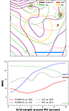 |
Fig. 3. Top: Density contours in 10″ × 10″ area centred on peak of M2 substructure recovered at RA = 64.03071, Dec = –24.07974 in PCANUCS. Spacing between contours is Δlog10κ = 0.05. The three primary lens models discussed in this article using the 303 images reported by R25 are shown in solid purple (PCANUCS), dashed green (L25), and dotted red (R25). The solid yellow circle denotes M2 with radius of 2.5″ corresponding to its characteristic radius. Bottom: Median percent difference (MPD) between models as a function of the length of the grid comparison window centred at about M2. Comparisons among PCANUCS and R25 (solid red), L25 and R25 (dash-dotted green), and PCANUCS and L25 (dashed blue) are shown. To compare these with the earlier works, the comparison using 237 images between P25 and B23 (dotted black) is also shown. For the comparisons between GRALE and LENSTOOL models, the solid horizontal dashes on the right indicate the MPD over the whole cluster for PCANUCS and R25 (red), PCANUCS and L25 (blue), L25 and R25 (green), and P25 and B23 (black). We note that the apparent misalignment of the contours near the galaxy positions is a likely side effect of interpolation using models of varying resolution. These shifts are restricted to the pixel level and have a negligible effect on our results. |
Interestingly, L25 and R25 disagree substantially at MPD ∼11% up to 6″ from M2. This is significant because L25 and R25 both use LENSTOOL and agree over the whole cluster with MPD of 2.63%. This is explained by the amplitude of the mass density reconstructed in both models. In the M2 region, the value of κ is lowest in R25 and highest in L25, with PCANUCS recovered between the two. The disagreement between L25 and R25 appears to be restricted to this region around M2, as the MPD substantially reduces on scales > 10″ to ∼8%. This local disagreement is likely to be due to the different prescriptions of both models in this area (Fig. 1). M2 is located in between the two large-scale DM clumps proposed by R25, whereas L25 assumes a single large-scale DM clump coincident with the BCG. In fact, L25 and R25 agree better on larger scales than PCANUCS does with either LENSTOOL model, which is consistent with the results of Perera et. al. (2025b) finding that parametric models are generally more similar to one another on cluster scales.
Up to the 10″ limit of the comparison around M2, we can conclude that R25 favours M2 more than L25 does since it exhibits consistent agreement better than the entire cluster over the entire 10″ grid area. That being said, neither LENSTOOL model reproduces a mass feature similar to PCANUCS. As has been shown, LENSTOOL always seems to prefer removing such a compact mass component in this region. The takeaway from this comparison experiment, therefore, is that the surface mass density around M2 exhibits agreement between GRALE and LENSTOOL at MPD ∼ 5–6%, which is better than over the entire cluster. However, the concentration of the density in this region remains unconstrained, with GRALE favouring a distinct mass substructure and LENSTOOL favouring a more diffuse mass distribution.
In other words, it appears that LENSTOOL wants to remove an explicit mass component at the M2 location, but that its surface mass density already features some mass at this location whose amount is close (within 5–6%) to that of the GRALE reconstruction. Therefore, while M2 is not favoured by the LENSTOOL parametric approach, it is not ruled out by it.
We note that we did not include the reconstruction by Diego et al. (2024b) in the model comparison near M2, as it relies on different inputs than those used in R25, L25, and PCANUCS, which could introduce a bias in the comparison. In particular, both the catalogue of multiple images and the catalogue of cluster members differ.
On the day before the formal acceptance of this paper, another study on MACS 0416 was submitted for publication (Cha & Jee 2025). The authors present a new hybrid SL modelling algorithm, MRMARTIAN, which they successfully tested on simulated data and applied to MACS 0416 using the 412 multiple images published by R25. This catalogue includes the 303 spectroscopically confirmed multiple images together with additional candidates. The convergence map from their reconstruction shows no indication of an overdensity at the M2 location (Cha & Jee 2025, private communication). A more detailed model comparison in the vicinity of M2 is not pursued here, given the timing of the publications and the differences in the sets of multiple images employed.
5. Conclusion
On galaxy-cluster scales, we have shown that we are able to describe the DM distribution in MACS 0416 with a DM traced by light model. We conclude that there is no need for any galaxy-cluster-scale LUMC in MACS 0416, since our model reproduces image positions just as well as the model with a LUMC (RMS of 0.57″ vs. 0.53″). This was already the case when using 182 multiple images (L22). We confirmed this finding using 303 multiple images. We note that we do not demonstrate that galaxy-cluster-scale LUMCs do not exist in MACS 0416, we only show that we do not need any to reproduce the multiple images, and we argue that this solution is more in tune with the theoretical expectations of structure formation and evolution.
On galaxy scales, we show that when considering 303 multiple images as constraints, a GRALE reconstruction still favours one LUMC instead of two when ‘only’ 237 multiple images were used. We have been testing this component parametrically with LENSTOOL, finding a mild local improvement of the RMS when explicitly including M2 in the modelling. Overall, LENSTOOL consistently wants to reject M2, whereas GRALE consistently favours M2. Still, we find that LENSTOOL models do also feature some mass in the M2 region, the value of which is close to the GRALE one (Fig. 3). Overall, we show that lens-model degeneracies remain important both on cluster and galaxy scales, despite the exquisite quality of the data.
We note that the intra cluster light component, which was not explicitly taken into account in this work, is known to be a diffuse component (see, e.g. Arnaboldi & Gerhard 2022; Montes & Trujillo 2022) distributed on scales larger than that of individual galaxies. It should therefore not be responsible for the M2 mass feature.
To conclude, we were able to propose a competitive parametric-mass model without the need for any LUMC in MACS 0416. We also present an updated GRALE model. These mass models and associated products are made publicly available for download at the Strong Lensing Cluster Atlas Data Base, which is hosted at the Laboratoire d’Astrophysique de Marseille2. This work provides further evidence for DM being associated with light at galaxy and galaxy-cluster scales. This association is loose, as discussed in the introduction. Finally, further investigations of the mass distribution at the M2 location is relevant.
The RMS difference of 0.04″ is of the same order of magnitude as the scatter in RMS values found when running the same model of MACS 0416 with different values of RATE and NB (see Table A.1). This difference is an order of magnitude smaller than the typical RMS error expected from image misidentification (Jauzac et al. 2016) or from unaccounted structure along the line of sight (Host 2012).
The optimized velocity dispersion for the foreground galaxy reported by R25 and L25 is 136±27 and 193±20 km/s (1σ error bars). Assuming a velocity dispersion equal to 165 km/s for this galaxy, it would generate a convergence κ of 0.006 at the location of M2. This is negligible compared to the reported κ value of 1.3 at M2, as evaluated from the optimized mass model and shown in Fig. 2. Considering the deflection angles is also relevant to demonstrate that the gravitational influence of this foreground galaxy is negligible. At the location and redshift of multiple image C2.3, it produces a deflection angle of 0.4″, which is smaller than the total RMS and negligible compared to the total deflection field of ∼16″ generated by the entire parametric model.
Acknowledgments
We thank the referee for a constructive report, and José Maria Diego for kindly sharing his κ map with us. ML acknowledges the Centre National de la Recherche Scientifique (CNRS) and the Centre National des Etudes Spatiale (CNES) for support. This work was performed using facilities offered by CeSAM (Centre de donnéeS Astrophysique de Marseille). Centre de Calcul Intensif d’Aix-Marseille is acknowledged for granting access to its high performance computing resources. DP acknowledges the computational resources provided by the Minnesota Supercomputing Institute, which were critical for this work. GR acknowledges support from the ERC Grant FIRSTLIGHT, the Slovenian national research agency ARIS through grants N1-0238 and P1-0188 and the European Space Agency through Prodex Experiment Arrangement No. 4000146646. This work is based on observations made with the NASA/ESA/CSA James Webb Space Telescope. The data were obtained from the Mikulski Archive for Space Telescopes at the Space Telescope Science Institute, which is operated by the Association of Universities for Research in Astronomy, Inc., under NASA contract NAS 5-03127 for JWST. These observations are associated with programs 1176 and 2738 (PEARLS; Windhorst et al. 2023) and program 1208 (CANUCS, DOI: 10.17909/18nv-np70; Sarrouh et al. 2025).
References
- Allen, S. W., Evrard, A. E., & Mantz, A. B. 2011, ARA&A, 49, 409 [Google Scholar]
- Arnaboldi, M., & Gerhard, O. E. 2022, ArXiv e-prints [arXiv:2212.09569] [Google Scholar]
- Beauchesne, B., Clément, B., Hibon, P., et al. 2024, MNRAS, 527, 3246 [Google Scholar]
- Bergamini, P., Rosati, P., Vanzella, E., et al. 2021, A&A, 645, A140 [EDP Sciences] [Google Scholar]
- Bergamini, P., Grillo, C., Rosati, P., et al. 2023, A&A, 674, A79 [NASA ADS] [CrossRef] [EDP Sciences] [Google Scholar]
- Bonamigo, M., Grillo, C., Ettori, S., et al. 2018, ApJ, 864, 98 [Google Scholar]
- Borgani, S., Murante, G., Springel, V., et al. 2004, MNRAS, 348, 1078 [Google Scholar]
- Cha, S., & Jee, M.J. 2025, ArXiv e-prints [arXiv:2508.13262] [Google Scholar]
- Despali, G., Giocoli, C., Bonamigo, M., Limousin, M., & Tormen, G. 2016, MNRAS, 466, 181 [Google Scholar]
- Diego, J. M., Li, S. K., Meena, A. K., et al. 2024a, A&A, 681, A124 [NASA ADS] [CrossRef] [EDP Sciences] [Google Scholar]
- Diego, J. M., Adams, N. J., Willner, S. P., et al. 2024b, A&A, 690, A114 [NASA ADS] [CrossRef] [EDP Sciences] [Google Scholar]
- Diego, J. M., Congedo, G., Gavazzi, R., et al. 2025, A&A, submitted [arXiv:2507.08545] [Google Scholar]
- Doppel, J. E., Jauzac, M., Lagattuta, D. J., Fattahi, A., & Mahler, G. 2025, ArXiv e-prints [arXiv:2506.09122] [Google Scholar]
- Elíasdóttir, Á., Limousin, M., & Richard, J. 2007, ArXiv e-prints [arXiv:0710.5636] [Google Scholar]
- Host, O. 2012, MNRAS, 420, L18 [NASA ADS] [CrossRef] [Google Scholar]
- Jauzac, M., Clément, B., Limousin, M., et al. 2014, MNRAS, 443, 1549 [Google Scholar]
- Jauzac, M., Jullo, E., Eckert, D., et al. 2015, MNRAS, 446, 4132 [Google Scholar]
- Jauzac, M., Eckert, D., Schwinn, J., et al. 2016, MNRAS, 463, 3876 [NASA ADS] [CrossRef] [Google Scholar]
- Jullo, E., Kneib, J.-P., Limousin, M., et al. 2007, New J. Phys., 9, 447 [Google Scholar]
- Liesenborgs, J., De Rijcke, S., & Dejonghe, H. 2006, MNRAS, 367, 1209 [NASA ADS] [CrossRef] [Google Scholar]
- Liesenborgs, J., de Rijcke, S., Dejonghe, H., & Bekaert, P. 2007, MNRAS, 380, 1729 [NASA ADS] [CrossRef] [Google Scholar]
- Liesenborgs, J., Williams, L. L. R., Wagner, J., & De Rijcke, S. 2020, MNRAS, 494, 3253 [NASA ADS] [CrossRef] [Google Scholar]
- Limousin, M., Kneib, J.-P., & Natarajan, P. 2005, MNRAS, 356, 309 [Google Scholar]
- Limousin, M., Richard, J., Jullo, E., et al. 2016, A&A, 588, A99 [NASA ADS] [CrossRef] [EDP Sciences] [Google Scholar]
- Limousin, M., Beauchesne, B., & Jullo, E. 2022, A&A, 664, A90 [NASA ADS] [CrossRef] [EDP Sciences] [Google Scholar]
- Limousin, M., Beauchesne, B., Niemiec, A., et al. 2025, A&A, 693, A33 [NASA ADS] [CrossRef] [EDP Sciences] [Google Scholar]
- Montes, M., & Trujillo, I. 2022, ApJ, 940, L51 [NASA ADS] [CrossRef] [Google Scholar]
- Perera, D., Jr., J. H. M. , Williams, L. L. R., et al. 2025a, Open J. Astrophys., 8, 37 [Google Scholar]
- Perera, D., Williams, L. L. R., Liesenborgs, J., et al. 2025b, MNRAS, 536, 2690 [Google Scholar]
- Richard, J., Claeyssens, A., Lagattuta, D., et al. 2021, A&A, 646, A83 [EDP Sciences] [Google Scholar]
- Rihtaršič, G., Bradač, M., Desprez, G., et al. 2025, A&A, 696, A15 [NASA ADS] [CrossRef] [EDP Sciences] [Google Scholar]
- Sarrouh, G. T. E., Asada, Y., Martis, N. S., et al. 2025, ArXiv e-prints [arXiv:2506.21685] [Google Scholar]
- Windhorst, R. A., Cohen, S. H., Jansen, R. A., et al. 2023, AJ, 165, 13 [NASA ADS] [CrossRef] [Google Scholar]
- Yoo, J., Shin, J., Hwang, H. S., et al. 2025, ApJ, 988, 229 [Google Scholar]
Appendix A: LENSTOOL mass model using 303 multiple images.
The updated LENSTOOL mass model presented in this paper is very similar to former LENSTOOL models discussed in this work, allowing easy comparison of their respective results. The cluster members are described in the modelling using scaling laws which have been constrained by spectroscopic observations (see B23 for more details). Two galaxies are optimized individually instead: one cluster member located near the northern BCG which is responsible for producing additional multiple images locally, and a foreground galaxy that perturbs the Southern giant arc. They are located at 47″ and 23″ from M2, respectively, and therefore have a negligible impact on M23. The X-ray gas component is explicitely taken into account by incorporating four dPIE mass clumps, which are not optimised, and whose values have been constrained by Bonamigo et al. (2018). The main difference between these mass models resides in the number of large scale DM clumps introduced in the modelling. The new one presented here and in L22 both do require that each large scale DM clump must be associated with a luminous counterpart, which sets the number of such clumps equal to three, whereas other studies propose four cluster scale DM mass clumps. In L22, contrary to the other studies discussed here, the ellipticity of each large scale DM clump was forced to be smaller than 0.7, motivated by the results from numerical simulations found for unimodal clusters (Despali et al. 2016). We here release this constraint, since MACS 0416 is far from being unimodal.
Two key parameters matter when it comes to the convergence of the LENSTOOL MCMC sampler (Jullo et al. 2007): the RATE parameter, associated to the burnin phase, and the number of iterations (NB), associated to the sampling phase. The smaller the rate, the more the sampler will move slowly to the high-likelihood areas and will be less prone to miss a mode of the posterior. The larger NB, the larger the number of iterations of the MCMC chains, the best the parameter space can be sampled. We refer the reader to (Limousin et al. 2025) for more details.
Former studies have used the following values for (RATE & NB): (0.05, 1000) in L22; (0.05, 100000) in B21 and B23 and (0.015, 10000) in R25. For our updated LENSTOOL mass model, we perform the (RATE, NB) test which was found to be useful to check if the parameters describing the mass distribution have actually converged (Limousin et al. 2025). In short, we lower the RATE and increase NB to see how it influences the RMS and the parameters of the mass clumps describing MACS 0416. Convergence is attained when the values for RATE & NB do not have any influence on the resulting RMS and on the parameters of the mass clumps. Table A.1 and Fig. A.1 show the results. We find that a RATE equal to 0.01 is small enough: PDFs corresponding to the different runs with RATE equal to 0.01 (black, grey and light grey) do agree with each other. This is not the case for runs with RATE equal to 0.05 (dark and light green), particularly for the NE clump, and, to a lesser extent, the South clump, while the Main clump is already well defined with a RATE equal to 0.05. Besides, when lowering the RATE to 0.005 (red/salmon), the results are in agreement with the one obtained with a RATE equal to 0.01. This suggest that, with RATE set to 0.01, the models have reached convergence. Regarding the NB parameter, we find that NB equal to 2000 (corresponding to 20 000 lines in the bayes.dat file) provides enough sampling. Comparing the different runs suggest that, when the RATE parameter is small enough, hence the area of the parameter space well defined, NB is of least importance, assuming it is large enough to provide a decent number of MCMC chains. 2000 is enough in this case. Our best model, in term of RATE & NB, is the one with RATE equal to 0.005 and NB equal to 5000. It is used to generate the different quantities presented in this paper. Its parameters are presented in Table A.2.
RMS obtained given different values of RATE & NB.
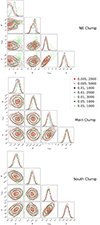 |
Fig. A.1. Corner plots obtained for the parameters of the mass model, for the values of RATE & NB indicated on the legend. Top: NE clump; middle: Main clump; bottom: South clump. The position of each clump is not shown for clarity since it is constrained to be coincident with the associated light component. |
We also compare the parameters obtained on the three DM mass clumps when the number of multiple images vary from 182 to 303. Green PDFs on Fig. A.2 correspond to models obtained when considering 182 multiple images, with: (RATE, NB) = (0.01, 1000; dark green) and (RATE, NB) = (0.01, 2000; light green). In both cases, the RMS is equal to 0.50″. Grey/black PDFs corresponds to models obtained when considering 303 multiple images, with (RATE, NB) = (0.01, 1000): black, (RATE, NB) = (0.01, 2000): grey, and (RATE, NB) = (0.01, 3000): light grey. In all cases, the RMS is equal to 0.58″.
We can appreciate how the constraints evolve when moving from 182 to 303 images. PDFs are tighter with 303 images and their position can vary a bit. Regarding the north-east Clump, we see that with 303 images, its parameters are much better defined than with 182 images.
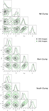 |
Fig. A.2. Corner plots obtained for the parameters of the mass model when considering 182 multiple images (green) and 303 multiple images (black/grey). A RATE of 0.01 is used for all realisations. |
dPIE parameters inferred for our best model of MACS 0416.
Appendix B: GRALE mass model using 303 multiple images.
We present on Fig. B.1 the projected surface mass density of our updated GRALE model obtained when using 303 multiple images as constraints.
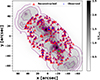 |
Fig. B.1. Projected surface mass density for the updated GRALE model. The observed image positions from R25 are shown as blue dots, while the reconstructed image positions are shown as red triangles. Only the M2 LUMC from the original model is reproduced and labelled in green. Contour lines are separated by Δκ = 0.25 in surface mass density. |
All Tables
All Figures
|
Fig. 1. Core of MACS 0416 from JWST data. North is up, east is left. We show the location of the cluster-scale DM clumps inferred in different studies by ellipses whose semi-axes are equal to the 3σ error bars on the position of these clumps: in yellow for Bergamini et al. (2021), in cyan for Bergamini et al. (2023), and in red for Rihtaršič et al. (2025). Green boxes represent the prior on the position of each cluster-scale DM clumps proposed by Limousin et al. (2022) and investigated in this work. In magenta, we show the location of the two galaxy-scale light-unaffiliated mass clumps inferred by Perera et al. (2025b). In white, we show the 303 secure multiple images reported by Rihtaršič et al. (2025). |
| In the text | |
|
Fig. 2. Core of MACS 0416 from JWST data. We show the total convergence maps for all models: B21 in yellow; B23 in cyan; R25 in red; our updated GRALE model (PCANUCS) in magenta; and our updated LENSTOOL model (L25) in green. We also show the convergence map from Diego et al. (2024b) in white (D24). We show the location of M2 in blue. |
| In the text | |
|
Fig. 3. Top: Density contours in 10″ × 10″ area centred on peak of M2 substructure recovered at RA = 64.03071, Dec = –24.07974 in PCANUCS. Spacing between contours is Δlog10κ = 0.05. The three primary lens models discussed in this article using the 303 images reported by R25 are shown in solid purple (PCANUCS), dashed green (L25), and dotted red (R25). The solid yellow circle denotes M2 with radius of 2.5″ corresponding to its characteristic radius. Bottom: Median percent difference (MPD) between models as a function of the length of the grid comparison window centred at about M2. Comparisons among PCANUCS and R25 (solid red), L25 and R25 (dash-dotted green), and PCANUCS and L25 (dashed blue) are shown. To compare these with the earlier works, the comparison using 237 images between P25 and B23 (dotted black) is also shown. For the comparisons between GRALE and LENSTOOL models, the solid horizontal dashes on the right indicate the MPD over the whole cluster for PCANUCS and R25 (red), PCANUCS and L25 (blue), L25 and R25 (green), and P25 and B23 (black). We note that the apparent misalignment of the contours near the galaxy positions is a likely side effect of interpolation using models of varying resolution. These shifts are restricted to the pixel level and have a negligible effect on our results. |
| In the text | |
|
Fig. A.1. Corner plots obtained for the parameters of the mass model, for the values of RATE & NB indicated on the legend. Top: NE clump; middle: Main clump; bottom: South clump. The position of each clump is not shown for clarity since it is constrained to be coincident with the associated light component. |
| In the text | |
|
Fig. A.2. Corner plots obtained for the parameters of the mass model when considering 182 multiple images (green) and 303 multiple images (black/grey). A RATE of 0.01 is used for all realisations. |
| In the text | |
|
Fig. B.1. Projected surface mass density for the updated GRALE model. The observed image positions from R25 are shown as blue dots, while the reconstructed image positions are shown as red triangles. Only the M2 LUMC from the original model is reproduced and labelled in green. Contour lines are separated by Δκ = 0.25 in surface mass density. |
| In the text | |
Current usage metrics show cumulative count of Article Views (full-text article views including HTML views, PDF and ePub downloads, according to the available data) and Abstracts Views on Vision4Press platform.
Data correspond to usage on the plateform after 2015. The current usage metrics is available 48-96 hours after online publication and is updated daily on week days.
Initial download of the metrics may take a while.