| Issue |
A&A
Volume 703, November 2025
|
|
|---|---|---|
| Article Number | A28 | |
| Number of page(s) | 8 | |
| Section | Astrophysical processes | |
| DOI | https://doi.org/10.1051/0004-6361/202556244 | |
| Published online | 03 November 2025 | |
First look at Vela X-1 with XRISM
A simultaneous campaign with XMM-Newton and NuSTAR
1
European Space Agency (ESA), European Space Astronomy Centre (ESAC), Camino Bajo del Castillo s/n, 28692 Villanueva de la Cañada, Madrid, Spain
2
IRAP, Université de Toulouse, CNRS, CNES, UT3-PS, Toulouse, France
3
Institut für Astronomie und Astrophysik, Universität Tübingen, Sand 1, 72076 Tübingen, Germany
4
Quasar Science Resources SL for ESA, European Space Astronomy Centre (ESAC), Science Operations Department, 28692 Villanueva de la Cañada, Madrid, Spain
5
INAF-Osservatorio Astronomico di Roma, Via Frascati 33, I-00078 Monte Porzio Catone, (RM), Italy
⋆ Corresponding author: This email address is being protected from spambots. You need JavaScript enabled to view it.
Received:
3
July
2025
Accepted:
3
September
2025
Abstract
Context. High-mass X-ray binaries (HMXBs) can serve as useful laboratories for exploring the behaviour of accreted matter onto compact objects and for probing the complex wind environments of massive stars. These investigations are essential for understanding stellar life cycles and the dynamics of the Milky Way, and they are prominent topics in the science cases for XRISM and NewAthena.
Aims. We report, for the first time, on a XRISM observation of the HMXB Vela X-1, conducted during the first cycle of the XRISM general observer programme and complemented by simultaneous XMM-Newton and NuSTAR coverage. This campaign targeted a critical orbital phase – when the neutron star is in inferior conjunction – during which significant changes in absorption are expected.
Methods. We performed absorption-resolved spectral analyses during two time intervals of interest: the soft and hard hardness ratio (HR) intervals, as it is strongly correlated with absorption variability.
Results.We observed a sudden transition in the HR from a soft to a hard state coinciding with an increase in the absorption column density. This is likely attributable to the onset of the accretion structure crossing our line of sight. With XRISM/Resolve, we also investigated the Fe K region, and we report for the first time the presence of a Fe Kα doublet in the spectrum of Vela X-1 together with the presence of already known Fe Kβ and Ni Kα lines that are produced in cold clumps embedded in the hot ionised wind. The measured line velocities of the order of 102 km s−1 are consistent with production sites in the vicinity of the neutron star.
Conclusions.This precursor study with Vela X-1 shows the potential of XRISM to study in unprecedented detail the spectral evolution of wind-accreting X-ray binaries.
Key words: stars: neutron / stars: winds / outflows / X-rays: binaries
© The Authors 2025
 Open Access article, published by EDP Sciences, under the terms of the Creative Commons Attribution License (https://creativecommons.org/licenses/by/4.0), which permits unrestricted use, distribution, and reproduction in any medium, provided the original work is properly cited.
This article is published in open access under the Subscribe to Open model. This email address is being protected from spambots. You need JavaScript enabled to view it. to support open access publication.
1. Introduction
Vela X-1 is an archetypal eclipsing high-mass X-ray binary (HMXB), and as it is located at only  kpc away (Kretschmar et al. 2021), it is one of the brightest persistent point sources in the X-ray sky despite its moderate average intrinsic luminosity of ∼5×1036 erg s−1 (Fürst et al. 2010). This system has been extensively reviewed by Kretschmar et al. (2021), who provide a comprehensive overview of its parameters. Vela X-1 comprises a B0.5 Ib supergiant star, HD 77581 (Hiltner et al. 1972), and an accreting neutron star in a close quasi-circular orbit with a period of ∼8.964 days (Kreykenbohm et al. 2008; Falanga et al. 2015). A dense stellar wind with
  (see e.g. Watanabe et al. 2006) feeds the neutron star, producing pulsed X-ray emission with a variable period of ∼283 s. Edge-on systems such as Vela X-1 (i > 73°, van Kerkwijk et al. 1995) enable orbital phase-resolved spectroscopy to probe different structures and regions in the stellar wind that are modified by interaction with the neutron star. Variations in the hydrogen absorption column density, NH, on our line of sight – a direct tracer of the stellar wind – show a post-eclipse decline until ϕorb ≈ 0.2–0.3 (Martínez-Núñez et al. 2014). This decline in absorption is followed by a rise in the 0.4–0.6 range, and it was first detected by Ohashi et al. (1984) and more recently monitored with high time resolution by Diez et al. (2023). At this range, the NH seems to stabilise at high values until the eclipse (Abalo et al. 2024). Local extrema attributed to the presence of clumps often modify this pattern and create rapid flux and spectral variability in Vela X-1 (Grinberg et al. 2017; Diez et al. 2023). Hydrodynamic simulations (Manousakis 2011) together with prior observations (Grinberg et al. 2017) have shown that an accretion wake trails the neutron star, and this is possibly caused by its supersonic motion around the companion star. In addition, the X-ray photoionisation from the compact object produces a large-scale filamentary wake (Blondin et al. 1990) known as the photoionisation wake. When these wakes intersect our line of sight, they absorb soft photons and reveal ionised emission lines in the Ne, S, Mg, and Si regions as well as Fe Kα, Kβ, and Ni Kα fluorescent lines (Sako et al. 1999; Goldstein et al. 2004; Martínez-Núñez et al. 2014; Amato et al. 2021). A public early release (ER) of a 64 ks XRISM observation of Vela X-11 at ϕorb ≈ 0.68–0.90 (see Fig. 1), not yet published in a journal, showcases fluorescent lines in the 6–8 keV band, including the Fe Kα1/Kα2 doublet and Fe Kβ line, and the ionised Fe XXV triplet.
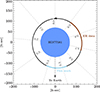 |
Fig. 1. Sketch of the Vela X-1 system showing the orbital phases covered by the neutron star during our XRISM observation (light blue) and during the ER observation (dark brown). In this image, the observer is facing the system at the bottom of the picture, and ϕorb = 0 is defined at the eclipse. |
In our targeted XRISM observation, we aimed to cover the inferior conjunction of the neutron star (see Fig. 1). At these phases, the passage of the accretion and ionisation wakes along the line of sight was observed in an earlier XMM-Newton and NuSTAR campaign (Diez et al. 2023). Monitoring this orbital phase enables measurement of the change in absorption column density at low energies as the wakes cross our line of sight. To constrain the high-energy continuum and compensate for the energy range not accessible to XRISM/Resolve due to the closed gate valve (see Sect. A in the Appendix), we requested simultaneous observations with NuSTAR and XMM-Newton.
2. Observations and data reduction
This coordinated observation of Vela X-1 with XRISM (Tashiro et al. 2025), NuSTAR (Harrison et al. 2013), and XMM-Newton (Jansen et al. 2001) was conducted on 19 November 2024. We used the European Photon Imaging Camera pn-CCD (EPIC-pn; Strüder et al. 2001) operated in timing mode on XMM-Newton. For NuSTAR, data were obtained with the Focal Plane Modules A and B (FPMA and FPMB). Finally, regarding XRISM, we employed the high-resolution X-ray imaging spectrometer Resolve and the soft X-ray imager Xtend (Tashiro et al. 2025) configured in the 1/8 window mode with 0.1 s burst mode. Further details of the observations are provided in Table A.1 in the Appendix, and a sketch of the Vela X-1 system showing the orbital phases we covered is shown in Fig. 1. We present in Appendix A in the Appendix a short description of the specific data reduction that has been applied for XMM-Newton/EPIC-pn in timing mode and technical details encountered during the XRISM/Resolve data acquisition.
The data analysis was performed using jaxspec v0.3.0 (Dupourqué et al. 2024). This X-ray spectral analysis Python library leverages the use of differentiable approaches for Bayesian inference, such as variational inference (see e.g. Blei et al. 2017), thus enabling thawing of all the parameters of the spectral model, and it provides robust constraints within short timescales. The models were fitted with variational inference with a multivariate Gaussian guide for the posterior parameters and adjusted using the Adam optimiser (Kingma & Ba 2017) with a learning rate of 10−3. We sought to minimise a Poisson likelihood for the observed spectrum, including a model-free background to account for its intrinsic uncertainty. We also used the Interactive Spectral Interpretation System (ISIS) v1.6.2-53 (Houck & Denicola 2000) for comparison and sanity checks with jaxspec and for plots. Both ISIS and jaxspec provide access to XSPEC (Arnaud 1996) models, which are referenced later in the text.
3. Results
3.1. Timing analysis
Vela X-1 is known for its strong flux variability on multiple timescales, from kiloseconds to individual neutron star pulses (see e.g. Martínez-Núñez et al. 2014; Diez et al. 2022, 2023). To examine the source’s variability during our observation, we present in Fig. 2 the 0.5–10 keV XMM-Newton/EPIC-pn, 5–79 keV NuSTAR, 2–10 keV XRISM/Resolve, and 0.5–10 keV XRISM/Xtend light curves. The pulse period (P) of Vela X-1 was independently determined using the Z2 statistics (Buccheri et al. 1983), based on photon events. We collected the photon events from all the instruments and corrected them for both barycentric motion and binary orbital effects using the orbital solution set by the Fermi Gamma-ray Burst Monitor Accreting Pulsars Program (Malacaria et al. 2020). The results are consistent, yielding a period of P = 283.595 ± 0.025 s. The light curves shown in Fig. 2 were binned accordingly to mitigate flux variations during one pulse cycle. The same Figure also shows the hardness ratio (HR) between the 0.5–3.0 keV and 8.0–10.0 keV energy bands. Two distinct phases are apparent in the HR: a soft HR interval and a hard HR interval. The HR serves as a reliable proxy for the absorption level in sources of this type (e.g. Abalo et al. 2024). In particular, a sharp transition from soft to hard HR was observed at ϕorb ≈ 0.463 in Fig. 2, which is typically attributed to the onset of accretion and ionisation wakes entering our line of sight, leading to increased absorption and spectral hardening (see detailed analysis in Diez et al. 2023).
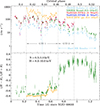 |
Fig. 2. Light curves and hardness ratio for XRISM/Resolve (light blue) and Xtend (green), XMM-Newton/EPIC-pn (orange), and NuSTAR/FPMA (red) and FPMB (blue) with a time resolution of P = 283.595 s. Top panel: Overall count rates in the energy bands corresponding to the respective instruments. The black dashed vertical lines denote the two GTIs we chose for our spectral analysis (Sect. 3.2 and Sect. 3.3). The dash-dotted light blue line marks the end of the FW electronics error, i.e. the beginning of the well-calibrated XRISM/Resolve data for our spectral analysis (Sect. 3.4). Bottom panel: Hardness ratio between the 0.5–3 keV (soft) and 8–10 keV (hard) energy bands. |
3.2. Soft HR (GTI 1): XMM-Newton + NuSTAR + XRISM
For the soft HR interval, we selected the good time interval (GTI) during which both low- and high-energy data are simultaneous. This corresponds to the interval from ∼60633.23 MJD (ϕorb ≈ 0.410) to ∼60633.71 MJD (ϕorb ≈ 0.463), referred to as ‘GTI 1’ in Fig. 2. This selection ensured constraints on the high-energy continuum while allowing us to investigate absorption variability at lower energies. Due to the filter wheel (FW) electronics error that compromised XRISM/Resolve data before ∼60633.47 MJD (see Fig. 2 and Appendix A), we excluded Resolve data before that MJD for this analysis. Since the XMM-Newton/EPIC-pn CCD camera already covers the 0.5–10 keV band and XRISM/Xtend operated with only ∼12% live-time (see Table A.1), we excluded Xtend from our analysis. This choice simplifies the spectral modelling by avoiding additional cross-calibration uncertainties beyond those already documented between XMM-Newton and NuSTAR (see Appendix in Diez et al. 2023). These will be addressed in a future study that is currently in preparation.
To maintain consistency with previous studies (Fürst et al. 2014; Diez et al. 2022, 2023), we adopted a partial covering model modified by a Fermi-Dirac high-energy cut-off (FDcut; Tanaka 1986) that can be written as
 (1)
(1)
where:  , TbabsISM = exp−NH, ISM σ(E), Tbpcf = CF × exp−NH σ(E) + (1 − CF).
Here, NH is left free to vary and represents the equivalent hydrogen column density of the dense stellar wind surrounding the neutron star. The interstellar medium (ISM) column density, NH, ISM, is fixed at 3.71 × 1021 cm−2 based on the NASA HEASARC NH tool (Ben Bekhti 2016). Abundances are from Wilms et al. (2000), and the cross-section σ is from Verner et al. (1996). The covering fraction (CF), ranging from zero to one, quantifies the opacity of the obscuring material. To correct for known calibration uncertainties in the EPIC-pn timing mode (e.g. Diez et al. 2023; Lai et al. 2024) and additional discrepancies with XRISM/Resolve, we introduced two cross-calibration normalisation constants, 𝒞EPIC − pn and 𝒞Resolve. We also accounted for discrepancies between NuSTAR’s FPMA and FPMB with 𝒞FPMB, setting FPMA as the reference for all detectors.
Three multiplicative broad Gaussian absorption components (Gabs) were used to model the two cyclotron resonance scattering features (CRSFs) and the 10-keV absorption feature. For additional emission or absorption lines, we used a phenomenological approach by fitting Gaussian components when significant residuals are present. Instead of judging the fit only in the sample or relying on asymptotic penalties (e.g. Akaike Information Criterion), we compared the expected log pointwise predictive density (elpd), as implemented in ArviZ (Vehtari et al. 2015), between models with and without line components. For this GTI 1, we detected five emission lines. Three lines are associated with the fluorescent Fe Kα2, Fe Kα1, and Fe Kβ transitions at around 6.39 keV, 6.40 keV, and 7.06 keV, respectively (Hölzer et al. 1997). These lines arise from photoionisation of Fe atoms with subsequent transitions from the L-shell and M-shell down to the K-shell producing the Kα doublet and the Kβ line, respectively. We also observed residuals around 1 keV and 1.3 keV corresponding to unresolved blended ionised lines in the Ne and Mg regions, which are typically associated with the presence of an ionised plasma around the X-ray source (e.g. Amato et al. 2021). We display in Fig. B.1 in the Appendix the simultaneous NuSTAR, XMM-Newton/EPIC-pn, and XRISM/Resolve spectra along with our best-fit model. We report in Table C.1 in the Appendix the corresponding parameter values. Although we can place upper limits on the normalisation and width of the fluorescent Ni Kα transition at ∼7.45 keV (Hölzer et al. 1997), the values are mostly consistent with zero. Moreover, including the Ni Kα line emission does not improve the elpd sufficiently to claim a detection (see inset of Fig. B.1).
Focusing on the stellar wind parameters obtained during this GTI 1, the covering fraction CF is  , and the equivalent hydrogen absorption column density of the stellar wind, NH, is
  . These values are consistent with the previous results reported by Diez et al. (2023), which were also obtained at a similar ϕorb (∼0.5) and soft HR interval.
We note that physically motivated reflection models have also been used to describe the complex wind geometry of Vela X-1, such as pexrav in Rahin & Behar (2023) or MYTORUS in Tzanavaris & Yaqoob (2018). However, Rahin & Behar (2023) argued that reflection from the star’s photosphere alone is not sufficient to explain discrepancies they observed at ϕorb ≈ 0.3–0.7 using NICER observations and that additional reflection may originate from clumps and from the accretion stream at these orbital phases. Additionally, Tzanavaris & Yaqoob (2018) conclude that the spectrum of the Chandra observation they analysed at ϕorb ≈ 0.5 is no longer reflection dominated, in contrast to another observation taken during the eclipse. A thorough investigation of the aforementioned models along with other physically motivated models for accreting X-ray pulsars available in the literature (e.g. compmag in Farinelli et al. 2016) in the context of our dataset is beyond the scope of this work. We note that our phenomenological approach employing a partial covering model supports the presence of a non-uniform and complex wind geometry, which is consistent with most of the literature, regardless of whether the data were modelled using physical or phenomenological approaches.
3.3. Hard HR (GTI 2): XRISM + NuSTAR
As in Sect. 3.2, we selected low- and high-energy simultaneous events during the hard HR interval, excluding XRISM/Xtend. For this GTI, no XMM-Newton coverage is available. Hence, we considered simultaneous NuSTAR and XRISM/Resolve data between ∼60633.71 MJD (ϕorb ≈ 0.463) and ∼60633.96 MJD (ϕorb ≈ 0.490), referred to as ‘GTI 2’ in Fig. 2.
We show in Fig. B.2 in the Appendix the NuSTAR and XRISM/Resolve simultaneous spectra with our best-fit model. We list in Table C.1 the corresponding parameter values. In this GTI 2, we detected three emission lines corresponding again to the Fe Kα2, Fe Kα1, and Fe Kβ fluorescent lines. As in GTI 1, the normalisation and width values of the Ni Kα line are consistent with zero with no strong detection (see inset of Fig. B.2). The previously detected soft lines below 2 keV in GTI 1 are not visible in this GTI 2. This is a consequence of the Resolve’s closed GV, the absence of XMM-Newton coverage, and our decision to exclude Xtend due to drastically reduced exposure time.
Focusing on the stellar wind influence during this GTI 2, we obtained a covering fraction CF of 0.882 ± 0.008 and an equivalent hydrogen absorption column density of the stellar wind NH of  . As in GTI 1, the CF remains close to one, indicating that almost 100% of the line of sight is obscured when the neutron star is near inferior conjunction. However, during GTI 2, the stellar wind NH is approximately three times higher than in GTI 1, which is consistent with the observed hardening of the spectral shape (Fig. 2) and likely due to increased absorption as reported by Abalo et al. (2024) with 14 years of MAXI data. This high absorption is also evidenced by the presence of the Fe K-edge at ∼7.1 keV in the Resolve spectrum, a feature that becomes more prominent with a high NH (see Fig. 3 in Diez et al. 2023).
3.4. Hard HR XRISM averaged spectrum
In order to have a look at the full XRISM/Resolve spectrum during the highly absorbed phase without constraints of GTI selection (Fig. 2), we show in Fig. 3 the XRISM/Resolve spectrum averaged over the full hard HR interval. This stable and long time interval mitigates variations caused by the high variability of the source and enhances the visibility of ionised lines in the spectrum thanks to a higher absorption. Hence, it allows for a deeper and pertinent investigation of the presence of line components in the Fe region. The continuum model we used here is our best-fit model from Eq. (1) with the parameters not covered by Resolve removed, such as the FDcut and CRSFs. We present the best-fit parameters in Table C.1 in the Appendix, and our search for line components is described in the following subsections.
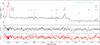 |
Fig. 3. Folded XRISM/Resolve spectrum (light blue) averaged over the hard HR interval. The red solid line corresponds to the base model we used to test for the presence of additional line components, indicated by the grey solid line (see Sect. 3.4.2). Lines for which a detection could be resolved are labelled by their names; the others are labelled by numbers. The corresponding ratio residuals in the lower panels are computed as data/model. For plotting purposes, the data were binned to a minimum of 150 counts/bin. |
3.4.1. Search for a Compton shoulder
When investigating the presence of a Compton shoulder (CS), we started by looking in the Fe lines, a feature that can be observed in HMXBs and that shows a strong Fe Kα complex (see e.g. Watanabe et al. 2003, for GX 301–2). When a high-energy photon propagates through matter, it has a non-negligible probability of interacting with electrons via Compton scattering. In this process, the photon loses energy (down-scattering), and if the original photon belongs to a strong emission line, this can produce a discernible Compton shoulder on the low-energy side of the observed line. We thus tied the energies of two Gaussian components to the Fe Kα1 and Kα2 line energies with a 156 eV offset as expected from the Compton formula (Watanabe et al. 2003). When comparing the elpd between models with and without the tied Gaussians, we did not observe any significant improvement of the fit with the addition of the CS, and the upper normalisation values are consistent with zero. We also tested a skewed Gaussian for the Fe Kα2 line in case of a very weak CS, but the results led to the same conclusion. Hence, we did not include a CS component in our model.
3.4.2. Line detections in the Fe region
We also searched for the presence of other emission or absorption line components in the Fe region. We fit Gaussian components with centroids close to reference energies of known transitions based on the database compiled by Hell et al. (2025) and where residuals are observed in the spectrum. The identification of spectral lines is uncertain and often ambiguous since many observed features could result from blends of unresolved fine-structure transitions or overlapping contributions from multiple ionisation states. The line components we tested are indicated in Fig. 3 by the grey line and corresponding numbers. In Fig. 4, we compare the elpd between the ‘base’ model, which consists of our best-fit continuum and includes previous confidently detected lines in this work (Fe Kα1, Fe Kα2, and Fe Kβ), and the same model adding one line at a time as labelled in Figs. 3 and 4. We observed that adding Line 12, which coincides well with the fluorescent Ni Kα complex, yielded the largest improvement to the base model. In contrast to GTI 1 and GTI 2, this time we could constrain the Ni Kα parameters as shown in Table C.1. Nonetheless, this weak detection fails to yield a statistically significant improvement in the fit once uncertainties are accounted for, as can be seen in Fig. 4. Similarly, we cannot confidently claim any additional line detections in our dataset because of the low signal-to-noise ratio. This may result from a combination of a reduced exposure time due to the FW electronics error and a difference in orbital phase: the ER covered ϕorb ≈ 0.68–0.90 (see Fig. 1), where higher absorption of ∼50×1022 cm−2 is expected (Diez et al. 2022). At such phases, the ionisation wake becomes more prominent in our line of sight, enhancing the visibility of ionised lines in the spectrum (Diez et al. 2023), which may lead to a stronger ionised Fe XXV complex around 6.6–6.7 keV, as seen in the XRISM ER data.
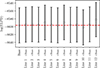 |
Fig. 4. Comparison of the expected log predictive densities between the base model and the same model adding one line component at a time. The base model includes the Fe Kα1, Fe Kα2, and Fe Kβ lines. |
If present, lines 1–2–3–4 coincide well with the He-like Fe XXV complex (w, x, y, z), and lines 6–7–8 coincide well with the H-like Fe XXVI complex (Lyα1 − 2 − 3) (Yerokhin & Surzhykov 2019; Yerokhin & Shabaev 2015). These emission lines are accompanied by absorption lines that could indicate a P-Cygni profile. Lines 11–12 likely correspond to the fluorescent Ni Kα2 and Kα1 transitions (Hölzer et al. 1997) in the Ni Kα complex. For lines 5–9–10, the identification is more uncertain. Although their energies match with Co Kα, Co XXVI w, and Cr XXIII w7, respectively (Hölzer et al. 1997; Yerokhin & Surzhykov 2019), the negligible abundances of Co and Cr compared to Fe, both in solar and ISM abundances (Wilms et al. 2000), make this interpretation very unlikely. These features could also result from blue- or red-shifted transitions of other elements. Due to insufficient statistics to confirm clear detections, we did not investigate the physical properties of these lines in this dataset further.
Looking at Table C.1, we noticed, as in GTI 2, that the energies of the fluorescent lines in the Fe region are found at their laboratory measurements (Hölzer et al. 1997), within the uncertainties. Hence, the observed broadening is likely due to turbulent motions in the wind and the intrinsic line shape for which the velocities can be derived by σline/Eline ≈ v/c for non-relativistic motions (v ≪ c) and computed using the posterior samples from the variational inference. We found  ,
,  ,
,  , and
, and  for the Fe Kα1, Fe Kα2, Fe Kβ, and Ni Kα lines, respectively.
4. Discussion and conclusion
The high resolving power of XRISM/Resolve provides new insights into the spectra of wind-accreting HMXBs, in particular their Fe region. Here, we have presented the results from a XRISM observation of Vela X-1 during the first cycle of the general observer programme complemented by simultaneous XMM-Newton and NuSTAR coverage. The line energies of the Fe Kα1 and Fe Kα2 doublet are consistent with near-neutral or lowly ionised ions (Fe XII or less, Kallman et al. 2004). Hence, observing strong fluorescent lines points towards a low to moderate ionisation state of the material despite an intense X-ray photoionisation, which is likely attributable to cold and dense clumps embedded in a hot and photoionised wind (Sako et al. 1999; Amato et al. 2021). In Chandra spectra at ϕorb ≈ 0.5, Goldstein et al. (2004) detected the additional fluorescent lines, such as Ni Kα and Fe Kβ, that we also observed in our XRISM/Resolve spectrum at the same orbital phase. We measured the wind velocities to be of the order of ∼102 km s−1 using the Fe Kα1, Fe Kα2, Fe Kβ, and Ni Kα lined broadening. These values are consistent with theoretical estimates of wind velocities in the inner region where the neutron star is located, according to Sander et al. (2018), who found v(dNS)≈100 km s−1. The velocity perturbations observed in the line-driven wind of hot stars create instabilities and subsequently turn into dense regions of gas, which explains the presence of clumps (see the review by Martínez-Núñez et al. 2017). Therefore, these near-neutral fluorescent lines were likely produced in cool clumps of gas in the vicinity of the neutron star during this observation, although Sato et al. (1986) and Watanabe et al. (2006) have also reported the presence of these lines further in the accretion wake with observations during the eclipse.
In this study, we have also demonstrated the pertinence and effectiveness of variational inference using the jaxspec X-ray spectral fitting library to produce meaningful constraints on the high-resolution spectra produced by XRISM/Resolve. All of the parameters of the fits were left to vary thanks to the use of variational inference with a multivariate Gaussian guide for the posterior parameters, which was not possible within the classical framework of ISIS for some parameters such as Ecut or Efold.
We detected a sudden increase in the HR, a behaviour already seen in Vela X-1 when the neutron star approaches an inferior conjunction around ϕorb ≈ 0.5 (Diez et al. 2023), which is attributed to the onset of the wakes crossing our line of sight. This transition occurs slightly earlier than in previous observations (Diez et al. 2023), confirming that the structures causing absorption variations are not stable in orbital phase. Future time-resolved spectroscopy tracking the evolution of the absorption column density, NH, will help constrain the presence and properties (e.g. mass, density) of clumps in the stellar wind. In this study, we have analysed only 79.3% of the total available NuSTAR exposure. We have not yet investigated the ∼6-ks XRISM/Xtend or the ∼42-ks XMM-Newton/RGS datasets, which will be addressed in a forthcoming publication.
https://heasarc.gsfc.nasa.gov/docs/xrism/results/erdata/index.html. The ER data can be used to prepare proposals for observing calls, but reliable scientific results cannot be derived from these data products until the full data and calibration are available.
Acknowledgments
We thank the anonymous referee for their valuable feedback which improved the quality of this work. CMD and EQ acknowledge support through the European Space Agency (ESA) Research Fellowship Programme in Space Science. SD acknowledges the support of CNRS/INSU and CNES. This project was provided with HPC and storage resources by GENCI at IDRIS thanks to the grant 2024-AD010416032 on the supercomputer Jean Zay’s A100/ H100 partitions. This work has made use of (1) the Interactive Spectral Interpretation System (ISIS) maintained by Chandra X-ray Center group at MIT; (2) the NuSTAR Data Analysis Software (NuSTARDAS) jointly developed by the ASI Science Data Center (ASDC, Italy) and the California Institute of Technology (Caltech, USA); (3) the ISIS functions (isisscripts; http://www.sternwarte.uni-erlangen.de/isis/) provided by ECAP/Remeis observatory and MIT; (4) NASA’s Astrophysics Data System Bibliographic Service (ADS). We thank John E. Davis for the development of the slxfig (http://www.jedsoft.org/fun/slxfig/) module used to prepare most of the figures in this work. This work made use of the JAX (Bradbury et al. 2018) and numpyro (Phan et al. 2019) packages.
References
- Abalo, L., Kretschmar, P., Fürst, F., et al. 2024, A&A, 692, A188 [NASA ADS] [CrossRef] [EDP Sciences] [Google Scholar]
- Amato, R., Grinberg, V., Hell, N., et al. 2021, A&A, 648, A105 [NASA ADS] [CrossRef] [EDP Sciences] [Google Scholar]
- Arnaud, K. A. 1996, ASP Conf. Ser., 101, 17 [Google Scholar]
- Bildsten, L., Chakrabarty, D., Chiu, J., et al. 1997, ApJS, 113, 367 [CrossRef] [Google Scholar]
- Blei, D. M., Kucukelbir, A., & McAuliffe, J. D. 2017, J. Am. Stat. Assoc., 112, 859 [CrossRef] [Google Scholar]
- Blondin, J. M., Kallman, T. R., Fryxell, B. A., & Taam, R. E. 1990, ApJ, 356, 591 [Google Scholar]
- Bradbury, J., Frostig, R., Hawkins, P., et al. 2018, JAX: composable transformations of Python+NumPy programs [Google Scholar]
- Buccheri, R., Bennett, K., Bignami, G. F., et al. 1983, A&A, 128, 245 [NASA ADS] [Google Scholar]
- de Vries, C. P., Haas, D., Yamasaki, N. Y., et al. 2018, J. Astron. Telescopes Instrum. Syst., 4, 011204 [Google Scholar]
- Diez, C. M., Grinberg, V., Fürst, F., et al. 2022, A&A, 660, A19 [NASA ADS] [CrossRef] [EDP Sciences] [Google Scholar]
- Diez, C. M., Grinberg, V., Fürst, F., et al. 2023, A&A, 674, A147 [NASA ADS] [CrossRef] [EDP Sciences] [Google Scholar]
- Dupourqué, S., Barret, D., Diez, C. M., Guillot, S., & Quintin, E. 2024, A&A, 690, A317 [NASA ADS] [CrossRef] [EDP Sciences] [Google Scholar]
- Falanga, M., Bozzo, E., Lutovinov, A., et al. 2015, A&A, 577, A130 [NASA ADS] [CrossRef] [EDP Sciences] [Google Scholar]
- Farinelli, R., Ferrigno, C., Bozzo, E., & Becker, P. A. 2016, A&A, 591, A29 [NASA ADS] [CrossRef] [EDP Sciences] [Google Scholar]
- Fürst, F., Kreykenbohm, I., Pottschmidt, K., et al. 2010, A&A, 519, A37 [CrossRef] [EDP Sciences] [Google Scholar]
- Fürst, F., Pottschmidt, K., Wilms, J., et al. 2014, ApJ, 780, 133 [Google Scholar]
- Goldstein, G., Huenemoerder, D. P., & Blank, D. 2004, AJ, 127, 2310 [Google Scholar]
- Grinberg, V., Hell, N., El Mellah, I., et al. 2017, A&A, 608, A143 [NASA ADS] [CrossRef] [EDP Sciences] [Google Scholar]
- Gülbahar, E. G., Diez, C. M., Ibarra, A., et al. 2025, Astron. Comput., 53, 100969 [Google Scholar]
- Harrison, F. A., Craig, W. W., Christensen, F. E., et al. 2013, ApJ, 770, 103 [Google Scholar]
- Hell, N., Brown, G. V., Eckart, M. E., et al. 2025, ArXiv e-prints [arXiv:2506.17106] [Google Scholar]
- HI4PI Collaboration (Ben Bekhti, N., et al) 2016, A&A, 594, A116 [NASA ADS] [CrossRef] [EDP Sciences] [Google Scholar]
- Hiltner, W. A., Werner, J., & Osmer, P. 1972, ApJ, 175, L19 [Google Scholar]
- Hölzer, G., Fritsch, M., Deutsch, M., Härtwig, J., & Förster, E. 1997, Phys. Rev. A, 56, 4554 [CrossRef] [Google Scholar]
- Houck, J. C., & Denicola, L. A. 2000, ASP Conf. Ser., 216, 591 [Google Scholar]
- Jansen, F., Lumb, D., Altieri, B., et al. 2001, A&A, 365, L1 [NASA ADS] [CrossRef] [EDP Sciences] [Google Scholar]
- Kaastra, J. S., & Bleeker, J. A. M. 2016, A&A, 587, A151 [NASA ADS] [CrossRef] [EDP Sciences] [Google Scholar]
- Kallman, T. R., Palmeri, P., Bautista, M. A., Mendoza, C., & Krolik, J. H. 2004, ApJS, 155, 675 [Google Scholar]
- Kingma, D. P., & Ba, J. 2017, Adam: A Method for Stochastic Optimization [Google Scholar]
- Kretschmar, P., El Mellah, I., Martínez-Núñez, S., et al. 2021, A&A, 652, A95 [NASA ADS] [CrossRef] [EDP Sciences] [Google Scholar]
- Kreykenbohm, I., Wilms, J., Kretschmar, P., et al. 2008, A&A, 492, 511 [NASA ADS] [CrossRef] [EDP Sciences] [Google Scholar]
- Lai, E. V., De Marco, B., Cavecchi, Y., et al. 2024, A&A, 691, A78 [NASA ADS] [CrossRef] [EDP Sciences] [Google Scholar]
- Malacaria, C., Jenke, P., Roberts, O. J., et al. 2020, ApJ, 896, 90 [NASA ADS] [CrossRef] [Google Scholar]
- Manousakis, A. 2011, Ph.D. Thesis, Université de Genève, Switzerland [Google Scholar]
- Martínez-Núñez, S., Torrejón, J. M., Kühnel, M., et al. 2014, A&A, 563, A70 [NASA ADS] [CrossRef] [EDP Sciences] [Google Scholar]
- Martínez-Núñez, S., Kretschmar, P., Bozzo, E., et al. 2017, Space Sci. Rev., 212, 59 [Google Scholar]
- Ohashi, T., Inoue, H., Koyama, K., et al. 1984, PASJ, 36, 699 [NASA ADS] [Google Scholar]
- Phan, D., Pradhan, N., & Jankowiak, M. 2019, ArXiv e-prints [arXiv:1912.11554] [Google Scholar]
- Porter, F. S., Chiao, M. P., Eckart, M. E., et al. 2016, J. Low Temp. Phys., 184, 498 [Google Scholar]
- Rahin, R., & Behar, E. 2023, ApJ, 950, 170 [Google Scholar]
- Sako, M., Liedahl, D. A., Kahn, S. M., & Paerels, F. 1999, ApJ, 525, 921 [Google Scholar]
- Sander, A. A. C., Fürst, F., Kretschmar, P., et al. 2018, A&A, 610, A60 [NASA ADS] [CrossRef] [EDP Sciences] [Google Scholar]
- Sato, N., Hayakawa, S., Nagase, F., et al. 1986, PASJ, 38, 731 [NASA ADS] [Google Scholar]
- Strüder, L., Briel, U., Dennerl, K., et al. 2001, A&A, 365, L18 [Google Scholar]
- Tanaka, Y. 1986, Proc. IAU Colloq. 89, 255, 198 [Google Scholar]
- Tashiro, M., Kelley, R., Watanabe, S., et al. 2025, PASJ, 77, 1 [Google Scholar]
- Tzanavaris, P., & Yaqoob, T. 2018, ApJ, 855, 25 [Google Scholar]
- van Kerkwijk, M. H., van Paradijs, J., & Zuiderwijk, E. J. 1995, A&A, 303, 497 [NASA ADS] [Google Scholar]
- Vehtari, A., Gelman, A., & Gabry, J. 2015, ArXiv e-prints [arXiv:1507.04544] [Google Scholar]
- Verner, D. A., Ferland, G. J., Korista, K. T., & Yakovlev, D. G. 1996, ApJ, 465, 487 [Google Scholar]
- Watanabe, S., Sako, M., Ishida, M., et al. 2003, ApJ, 597, L37 [NASA ADS] [CrossRef] [Google Scholar]
- Watanabe, S., Sako, M., Ishida, M., et al. 2006, ApJ, 651, 421 [Google Scholar]
- Wilms, J., Allen, A., & McCray, R. 2000, ApJ, 542, 914 [Google Scholar]
- Yerokhin, V. A., & Shabaev, V. M. 2015, J. Phys. Chem. Ref. Data, 44, 033103 [Google Scholar]
- Yerokhin, V. A., & Surzhykov, A. 2019, J. Phys. Chem. Ref. Data, 48, 033104 [Google Scholar]
Appendix A: Data reduction
Observations log.
The EPIC-pn observation is significantly affected by pile-up. To mitigate this, we use the epatplot tool, following the approach outlined in the Appendix of Diez et al. (2023). Specifically, we exclude the three centremost columns of the point spread function (PSF), RAWX 36–37–38, which are most severely impacted. A Jupyter Notebook tutorial for the XMM-Newton data extraction of another observation of Vela X-1 is provided in Gülbahar et al. (2025) and follows a procedure similar to the one used here. As reported in Diez et al. (2023), we also observe count-rate-dependent energy scale shifts in the EPIC-pn spectrum of Vela X-1, as evidenced by the Fe Kα line appearing at ∼6.56 keV instead of the expected 6.4 keV. Since the release of SAS v22.1.0, an updated version of the evenergyshift2 task has been made available3. Following the recommended procedure, we measured energy shifts in the time-averaged spectrum near the instrumental edges and applied the evenergyshift correction, which resulted in the Fe Kα line shifting to ∼6.42 keV. We did not need to filter for flaring particle background or extract a background, because the source was so bright that it illuminated the entire EPIC-pn focal plane.
Resolve is a soft X-ray spectrometer composed of a 6 × 6 array of microcalorimeters with an excellent spectral resolution of 4.5 eV FWHM at 6 keV (Tashiro et al. 2025). Unfortunately, the X-ray aperture door – known as the gate valve (GV) – remains closed despite several attempts to open it, effectively blocking soft X-rays below 2 keV and attenuating the overall bandpass. In addition, during our observation, a filter wheel (FW) electronics error (now resolved) prevented the planned rotation of the 55Fe FW calibration source (for more details, see Porter et al. 2016; de Vries et al. 2018), compromising the spectral data quality before ∼60633.47 MJD. Nevertheless, thanks to the high count rate of Vela X-1, we have sufficient photon statistics to meet most of our scientific objectives.
The orbital phases ϕorb mentioned in this work are derived from the ephemeris of Bildsten et al. (1997) and Kreykenbohm et al. (2008), as summarised in Table 1 of Diez et al. (2022), where ϕorb = 0 is defined as the time when the mean longitude l equals 90° (T90), following the convention commonly used for this source. All times are barycentred and corrected for the binary orbit. All spectra are rebinned using the optimal approach from Kaastra & Bleeker (2016), with an additional criterion of a minimum of 50 cts/bin for XRISM/Resolve due to the high statistics that is enabled by the instrument. Errors are given within 2-σ confidence level, unless stated otherwise. We use HEASOFT v6.35.1 for the reduction of data from the NASA-led missions NuSTAR and XRISM. For XMM-Newton data extraction, we use the Science Analysis System (SAS) software v22.1.0.
Appendix B: Spectra for GTI 1 and GTI 2
 |
Fig. B.1. Folded spectra for GTI 1 obtained with XMM-Newton/EPIC-pn (orange), NuSTAR/FPMA (red) and FPMB (dark blue), and XRISM/Resolve (light blue). Solid lines show the best-fit model and corresponding ratio in the bottom panel computed as data/model. A zoom in the Fe region is shown to highlight the resolution capabilities of Resolve. For plotting and readability purposes, the NuSTAR and XMM-Newton data are not displayed in the zoomed window and the XRISM/Resolve data are binned to a minimum of 150 counts/bin. |
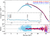 |
Fig. B.2. Folded spectra for GTI 2 obtained with XRISM/Resolve (light blue), and NuSTAR/FPMA (red) and FPMB (dark blue). Solid lines show the best-fit model and corresponding ratio in the bottom panel computed as data/model. A zoom in the Fe region is shown to highlight the resolution capabilities of Resolve. For plotting and readability purposes, the NuSTAR data are not displayed in the zoomed window and the XRISM/Resolve data are binned to a minimum of 150 counts/bin. |
Appendix C: Best-fit parameters
All Tables
All Figures
|
Fig. 1. Sketch of the Vela X-1 system showing the orbital phases covered by the neutron star during our XRISM observation (light blue) and during the ER observation (dark brown). In this image, the observer is facing the system at the bottom of the picture, and ϕorb = 0 is defined at the eclipse. |
| In the text | |
|
Fig. 2. Light curves and hardness ratio for XRISM/Resolve (light blue) and Xtend (green), XMM-Newton/EPIC-pn (orange), and NuSTAR/FPMA (red) and FPMB (blue) with a time resolution of P = 283.595 s. Top panel: Overall count rates in the energy bands corresponding to the respective instruments. The black dashed vertical lines denote the two GTIs we chose for our spectral analysis (Sect. 3.2 and Sect. 3.3). The dash-dotted light blue line marks the end of the FW electronics error, i.e. the beginning of the well-calibrated XRISM/Resolve data for our spectral analysis (Sect. 3.4). Bottom panel: Hardness ratio between the 0.5–3 keV (soft) and 8–10 keV (hard) energy bands. |
| In the text | |
|
Fig. 3. Folded XRISM/Resolve spectrum (light blue) averaged over the hard HR interval. The red solid line corresponds to the base model we used to test for the presence of additional line components, indicated by the grey solid line (see Sect. 3.4.2). Lines for which a detection could be resolved are labelled by their names; the others are labelled by numbers. The corresponding ratio residuals in the lower panels are computed as data/model. For plotting purposes, the data were binned to a minimum of 150 counts/bin. |
| In the text | |
|
Fig. 4. Comparison of the expected log predictive densities between the base model and the same model adding one line component at a time. The base model includes the Fe Kα1, Fe Kα2, and Fe Kβ lines. |
| In the text | |
|
Fig. B.1. Folded spectra for GTI 1 obtained with XMM-Newton/EPIC-pn (orange), NuSTAR/FPMA (red) and FPMB (dark blue), and XRISM/Resolve (light blue). Solid lines show the best-fit model and corresponding ratio in the bottom panel computed as data/model. A zoom in the Fe region is shown to highlight the resolution capabilities of Resolve. For plotting and readability purposes, the NuSTAR and XMM-Newton data are not displayed in the zoomed window and the XRISM/Resolve data are binned to a minimum of 150 counts/bin. |
| In the text | |
|
Fig. B.2. Folded spectra for GTI 2 obtained with XRISM/Resolve (light blue), and NuSTAR/FPMA (red) and FPMB (dark blue). Solid lines show the best-fit model and corresponding ratio in the bottom panel computed as data/model. A zoom in the Fe region is shown to highlight the resolution capabilities of Resolve. For plotting and readability purposes, the NuSTAR data are not displayed in the zoomed window and the XRISM/Resolve data are binned to a minimum of 150 counts/bin. |
| In the text | |
Current usage metrics show cumulative count of Article Views (full-text article views including HTML views, PDF and ePub downloads, according to the available data) and Abstracts Views on Vision4Press platform.
Data correspond to usage on the plateform after 2015. The current usage metrics is available 48-96 hours after online publication and is updated daily on week days.
Initial download of the metrics may take a while.