| Issue |
A&A
Volume 703, November 2025
|
|
|---|---|---|
| Article Number | A252 | |
| Number of page(s) | 14 | |
| Section | Extragalactic astronomy | |
| DOI | https://doi.org/10.1051/0004-6361/202556351 | |
| Published online | 19 November 2025 | |
Investigating galactic fountains in M101
Insights from UV emission, ionised gas, and neutral gas
1
Observatoire de Paris, LUX, CNRS, PSL University, Sorbonne University, 75014 Paris, France
2
Collège de France, 11 place Marcelin Berthelot, 75231 Paris, France
⋆ Corresponding author: This email address is being protected from spambots. You need JavaScript enabled to view it.
Received:
10
July
2025
Accepted:
30
September
2025
Abstract
Spiral galaxy disks are thought to exist in a quasi-stationary state, between fresh gas accretion from cosmic filaments and disk star formation, self-regulated through massive-star feedback. Our goal here is to quantify these feedback processes and probe their efficiency. While star formation can be traced at 10 Myr time-scales through Hα emission, the signature of OB stars, and at 100 Myr scale with UV emission, the gas surface density is traced by H I emission for the atomic phase. We chose to investigate feedback processes using fountain effects in M101, a nearby well-observed face-on galaxy. Face-on studies are complementary to the more frequent edge-on observations of these fountains in the literature. We use high-resolution data from THINGS for the H I emission, GALEX for UV, and SITELLE-SIGNALS for the Hα tracer. We identified 20 new H I holes, in addition to the 52 holes found in 1993. We study in more detail the nine holes satisfying strong criteria to be true fountain effects, compute their physical properties, and derive their energy balance. Only one small H I hole still contains Hα and young stars inside, while the largest hole of 2.4 kpc and the oldest age (94 Myr) is deprived of Hα and UV. For face-on disks, the possibility to study simultaneously the H I shell morphology, the stellar association, and kinematic evidence is of primordial importance. In M101, we quantified how stellar feedback is responsible for carving the observed cavities in the atomic gas disk, and how it can expel neutral gas above the disk, which is then unavailable for star formation during up to 100 Myr.
Key words: galaxies: evolution / galaxies: individual: M101 / galaxies: kinematics and dynamics / galaxies: spiral / galaxies: star formation
© The Authors 2025
 Open Access article, published by EDP Sciences, under the terms of the Creative Commons Attribution License (https://creativecommons.org/licenses/by/4.0), which permits unrestricted use, distribution, and reproduction in any medium, provided the original work is properly cited.
This article is published in open access under the Subscribe to Open model. This email address is being protected from spambots. You need JavaScript enabled to view it. to support open access publication.
1. Introduction
Feedback processes are pivotal regulators of galaxy evolution, governing the baryon cycle between stars, the interstellar medium (ISM), and the circumgalactic medium. The interplay of gas accretion, outflow, and recycling controls star formation rates (SFRs), disk stability, and chemical enrichment (e.g. Somerville & Davé 2015). Stellar feedback, primarily from supernovae (SNe), stellar winds, and intense radiation fields, can expel metal-rich gas from the disk. When this gas cools and condenses after ejection, it can fall back and fuel subsequent star formation, forming a closed-loop mechanism known as the galactic fountain (Shapiro & Field 1976).
In the galactic fountain framework, clustered SN explosions and massive OB stellar winds heat the ISM to temperatures of order ∼106 K, launching gas vertically (upto 1 kpc, Shapiro & Field 1976) at velocities that may or may not exceed the galaxy’s escape speed. If the velocity is insufficient for escape, the ejected gas cools radiatively or mixes with cooler ISM phases, recombines into atomic hydrogen (H I), and can later form molecular clouds (H2) under favourable conditions (Bregman 1980). These clouds, often seen as high-velocity complexes such as those in the Milky Way (van Woerden et al. 1999) and M31 (Davies 1975; Westmeier et al. 2007), eventually rain back onto the disk with velocities ∼100 km s−1 (Shapiro & Field 1976) over timescales of ∼80–100 Myr (33 Myr for cooling and another 47 Myr to return to the disk, Houck & Bregman 1990). This cycle contributes to disk turbulence, redistributes metals, and regulates star formation over galactic scales (Armillotta et al. 2016).
Galactic fountains have been observed most directly in edge-on galaxies such as NGC 891 (i ≳ 89°; Oosterloo et al. 2007) and NGC 2403 (i ∼ 60°; Fraternali et al. 2002), where extra-planar H I and ionised gas trace vertical fountain flows above the plane. However, nearly face-on systems such as NGC 628 offer a complementary view. In such galaxies, vertical motions are largely hidden but the in-plane manifestations – H I holes, expanding shells, and luminous clusters in ultraviolet (UV) – can be identified in the disk as the launch sites of fountain activity (Kamphuis & Briggs 1992).
M101 (NGC 5457) is a nearby face-on spiral galaxy at a distance of 6.4 ± 0.7 Mpc (Shappee & Stanek 2011), with a modest inclination of 18° (Walter et al. 2008, see Table 1 for other properties). It hosts vigorous star formation (∼2.4 M⊙ yr−1; Leroy et al. 2013), a flocculent barred structure, and no prominent bulge. At its distance, 1″ corresponds to 31 pc see Table 1. Early H I studies by (Kamphuis 1993, henceforth K93) on this galaxy, using ∼15″ resolution Westerbork data, identified 52 H I holes and two high-velocity complexes. One of these holes, located on the outer disk, was interpreted as a superbubble requiring ∼1000 SNe to account for its energy (Kamphuis et al. 1991). More recently, Chakraborti & Ray (2011) discovered a distinct supershell in the inner disk of M101, traced by UV emission, likely powered by clustered SNe. These studies established M101 as a promising case for investigating stellar feedback and the resulting ISM structures.
Properties of galaxy M101 (NGC 5457) from the literature.
While UV, H I and ionised gas observations of M101 have each been studied independently, no systematic multi-wavelength attempt has been made to identify galactic fountain activity and form a complete view of the feedback loop. This study presents the first such effort: using high-resolution data from H I 21 cm, UV, and optical integral field unit (IFU) spectroscopy, we aim to identify observational signatures of galactic fountains in M101 from a face-on perspective.
The features we look for as signatures of galactic fountain activity span multiple wavelengths and gas phases. In the ultraviolet regime, we expect to detect compact star-forming complexes whose massive stars are capable of driving fountains via their stellar winds and SN explosions. These appear as clumps in the GALEX FUV intensity maps and trace recent massive star formation on ≲100 Myr timescales, compared to ≲10 Myr for Hα emission (Keel et al. 2004; Rampazzo et al. 2022). The UV thus provides a longer-baseline locator for potential fountain launch sites.
The SNe from these associations inject energy into the surrounding interstellar medium, driving outflows of hot, ionised gas. These can be traced with SITELLE kinematics via velocity-broadened or multi-peaked Hα profiles and with coherent morphologies such as shells and bubble-like structures in narrow-band maps (Camps-Fariña et al. 2017; Rupke 2018, and references therein). Recent PHANGS studies provide high-resolution, multi-phase benchmarks for feedback-driven bubbles: from molecular-gas measurements of sizes, expansion speeds, energetics and lifetimes (Watkins et al. 2023a), to energy-balance analyses linking the mechanical output of young massive stars with the kinetic energy of turbulent, ionised gas (Egorov et al. 2023), and a panchromatic, spatially resolved census of bubbles and their associated stellar populations in NGC 628 (Watkins et al. 2023b).
These energetic events also displace the atomic hydrogen that previously occupied the region. As a result, observations in the 21 cm line of H I often reveal these sites as gaps, depressions, or cavities in the atomic gas distribution. Such H I holes are commonly seen in nearby spiral galaxies (Brinks & Bajaja 1986; Deul & den Hartog 1990; Puche et al. 1992; Kamphuis 1993; Wilcots & Miller 1998; Fraternali et al. 2002; Boomsma et al. 2008; Bagetakos et al. 2011; Pokhrel et al. 2020), including the Milky Way (Heiles 1979, 1984; Hu 1981). While some of these holes appear to be genuine voids, others are known to be filled with either hot ionised gas or colder molecular material. Their physical origin can vary, but many are linked to disk processes such as clustered SN explosions, stellar winds, or, in some cases, gas infall from the halo or circumgalactic medium (e.g. Putman et al. 2012). A recent work by Lara-López et al. (2023) concluded that supernovae remnants (SNRs) concentrate on the rims of H I holes and can trigger star formation there.
Through this study, we aim to determine which disk cavities in M101 are consistent with feedback-driven fountains and to assess their sizes, possible ages, and implications for the cycling of gas between the disk and halo. We describe our data sources in Section 2 and methodology in Section 3. Our results are presented in Section 4, with their implications discussed in Section 5.
2. Data description
This study makes use of three archival, multi-wavelength datasets to trace young stellar populations, atomic hydrogen structures, and ionised gas morphology and kinematics, respectively. Figure 1 is a hybrid map combining atomic gas, ionised gas, and ultraviolet emission.
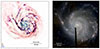 |
Fig. 1. Multi-wavelength views of NGC 5457 or M101. Left: False-colour RGB composite of M101 using H I (THINGS, red), Hα (SITELLE, green), and FUV (GALEX, blue). The colour mapping is subtractive rather than additive, highlighting variations in neutral gas phase (H I), recently star-forming regions (Hα), and older star formation (FUV). Right: False-colour RGB composite of M101 using SITELLE’s SN1, SN2, and SN3 filters. The mosaic combines four pointings (each covering 11′×11′) to capture the full extent of the galaxy. |
2.1. GALEX FUV and NUV
The Galaxy Evolution Explorer (GALEX, Martin et al. 2005) data used in this study were obtained from the Guest Investigator Cycle 3 with ID: GI3_050008_NGC5457 in the far-UV (FUV: 1500–1800 Å) and near-UV (NUV: 1750-2800 Å) bands, with exposure lengths of 13293.4 and 13294.4 seconds, respectively. These data were retrieved from the MAST Archive and have spatial resolutions of 4.3″ (FUV) and 5.3″ (NUV). For this analysis, we use the intensity maps (fd-int.fits.gz and nd-int.fits.gz), which are provided in units of counts s−1 pixel−1 with a pixel scale of 1.5″. These images are used primarily for morphological identification of UV-bright stellar associations near H I holes and SITELLE shells.
2.2. The H I nearby galaxy survey
The H I Nearby Galaxy Survey (THINGS, Walter et al. 2008), conducted using the NRAO Very Large Array, provides high-resolution 21 cm H I observations of nearby galaxies. We retrieved the data for M101 (NGC 5457) from the THINGS public archive1, along with its moment maps for integrated flux, velocity field, and velocity dispersion.
For our analysis, we used the data cube with natural weighting, which provides low noise and has a spectral resolution of 5.2 km s−1 with a total of 69 velocity channels. We also used the maps obtained from the cube of robust weighting to cross-check hole boundaries and structure in ambiguous cases, as it has higher resolution but also higher noise levels. The image dimensions are 2048 × 2048 pixels, with a pixel size of 1.0″. The root-mean-squared (RMS) noise in one channel map is 0.46 mJy beam−1, which corresponds to an H I column density sensitivity of ∼3.2 × 1020 cm−2. The synthesised beam size of the natural (respectively, robust) cube is 10.82″ × 10.17″ (7.49″ × 6.07″) with a position angle of −67.0° (−56.6° measured north to east; Walter et al. 2008).
Table 2 compares the observational properties of the original K93 dataset with the THINGS data used in this study.
Comparison of H I observational properties.
2.3. SIGNALS-SITELLE
M101 is one of the galaxies observed in the Star-formation, Ionised Gas, and Nebular Abundances Legacy Survey (SIGNALS; Rousseau-Nepton et al. 2019), conducted at the Canada-France-Hawaii Telescope (CFHT) using the Spectromètre Imageur à Transformée de Fourier pour l’Etude en Long et en Large de raies d’Emission (SITELLE) imaging spectrograph (Drissen et al. 2019). Because of its proximity and extent, the galaxy was observed across four fields with three spectral filters: SN1 (363–386 nm), SN2 (482–513 nm), and SN3 (647–685 nm), at spectral resolutions of 1000 for SN1 and SN2, and 5000 for SN3, where ‘SN’ stands for SITELLE Narrow-band. The reduced data, retrieved from the Canadian Astronomy Data Centre, is available as HDF5 files for each filter and field.
The emission lines covered comprise [O II] λλ3726, 3729 (SN1), Hβ at 4861 Å and [O III] λλ4959, 5007 (SN2), and Hα at 6563 Å, [N II] λλ6548, 6584, and [S II] λλ6717, 6731 (SN3). The deep frame, which comes with the data cube and is the sum of all individual interferometric frames, provides a high signal-to-noise image of the field per filter. Amosaic using these narrowband filters in the optical regime is shown in the right panel of Fig. 1.
The instrumental line shape of SITELLE is a cardinal sine (sinc) function, and the physical information of an emitting region is embedded in a sinc-Gauss (the result of the convolution of a sinc with a Gaussian) profile (Martin et al. 2016). We therefore analyse the SITELLE data cubes using Outils de Réduction de Cubes Spectraux (ORCS, Martin et al. 2015), a software designed for SITELLE data reduction and analysis. In this work, we used the ORCS-generated maps of flux, velocity and dispersion, along with their uncertainties, for the Hα and [S II] lines, which were produced after background subtraction and simultaneous fitting of a single sinc-Gauss profile to all emission lines in the SN3 data cube without any pixel binning. Accordingly, when referring to ‘Hα velocity’ or ‘Hα dispersion’ throughout this paper, we mean the velocity and dispersion maps derived from the global SN3 fit.
3. Methodology
In this section, we describe how regions hosting fountain-driven feedback features are identified using a multi-wavelength analysis of H I, ultraviolet, and ionised gas data. Following Bagetakos et al. (2011) and Pokhrel et al. (2020), we forgo automated H I-hole detection in favour of visual inspection owing to the irregular morphologies of H I structures in galaxy disks. We identified candidate galactic fountain sites in M101 via two approaches mentioned in Section 3.1, then subjected them to a scoring scheme in Section 3.2 to identify true holes driven by feedback, and finally estimated certain observed and derived properties as mentioned in Section 3.3 for each of these high-scoring sites hosting a galactic fountain.
3.1. Preliminary candidates
As a preliminary step, we constructed an initial catalogue of H I cavities in M101 using two complementary routes, before any assessment of whether these are bona fide feedback-driven holes (Section 3.2). Our goal at this stage was to identify all plausible cavity candidates visible in the H I moment-zero map, regardless of their eventual classification.
First, we revisited the 52 H I holes catalogued by K93 whose diameters range from ∼0.8 to 6.6 kpc. These were originally detected using data with ∼15″ resolution, limiting sensitivity to structures larger than ∼600 pc. With the improved resolution of the THINGS dataset (6″, corresponding to ∼200 pc at M101’s distance of 6.4 ± 0.7 Mpc; Shappee & Stanek 2011), we revisited these holes using higher-quality H I, SITELLE Hα, and GALEX UV data. To do so, we overlaid the positions and extents of the K93 holes as ellipses or circles on the THINGS H I moment maps, SITELLE Hα emission maps, and GALEX FUV intensity maps using CARTA (Comrie et al. 2021). Out of these 52 holes, one hole lies outside the THINGS field-of-view, so we drop it early on. The rest of these 51 structures are then subjected to a scoring scheme described in Section 3.2.
In the second approach, we started with a visual inspection of the SITELLE colour image given in the right panel of Fig. 1, which was produced from the individual SN1, SN2 and SN3 deep frames using the IRAFrgbsun routine (Tody 1986), with final adjustments made in GIMP2 by Laurent Drissen (private communication). Owing to the stratified, onion-like ionisation structure of photoionised nebulae (see e.g. Morisset 2018), and to the fact that each SN filter samples different ionisation lines, spatially resolved SITELLE-IFU data reveal distinct ionisation zones in such an RGB composite: low-ionisation lines dominate the outer rims, while higher-ionisation lines appear towards the interior. We exploit this to visually identify circular or elliptical rim- or bubble-like H II regions in the RGB image. Each candidate is then cross-matched with the GALEX FUV map to confirm the presence of a young stellar cluster inside or near the centre. Finally, we inspected the THINGS H I natural and robust moment-zero map at that location for a corresponding local minimum. This process yielded 20 new, generally smaller, cavity candidates. This approach also found back some of the previously-catalogued holes from K93.
Combining the two approaches, we obtained a preliminary set of 71 H I cavities. These are all subjected, in the next stage, to the uniform scoring procedure described in Section 3.2 to assess whether they are genuine holes and whether their properties are consistent with galactic fountain-driven origins. We also generated [S II]/Hα maps, as shock-ionised shells from SNR often exhibit elevated [S II]/Hα > 0.5.
3.2. Quality assurance scoring scheme
The scoring schemes of Bagetakos et al. (2011) and Pokhrel et al. (2020) were designed to identify H I holes, without explicitly distinguishing between those created by stellar feedback and those of dynamical origin. In this work, we adapt and extend their approach to ensure that only feedback-driven holes are selected, with additional criteria tailored to identifying sites of galactic fountain activity. Each hole is assigned points based on its morphological, kinematic, and multi-wavelength signatures, as depicted in Figure 2.
One point is assigned if the hole shows a well-defined flux minimum in the H I integrated flux map – quantified as a ≥50% drop in surface brightness in the line profile extracted along the position angle of the ellipse – suggesting coherent depletion (Panels a and b of Fig. 2). Another point is added if this depression remains spatially consistent across at least three consecutive channels in the THINGS data cube, helping to mitigate false positives caused by turbulence or noise. Additional points are given depending on the number of contiguous velocity-channels where the depression is seen: 1–2 (5–10 km s−1), 3–4 (11–20 km s−1), and > 4 (> 20 km s−1) channels receive +1, +2, and +3 points respectively. An extra point is added if the hole shows an elevated velocity dispersion in the H I moment-2 map compared to the local surroundings (Panel c in Figure 2). If the hole lies completely within a spiral arm, it receives +1, as spiral-arm holes are more likely to be star-formation-driven.
Next, we extracted position–velocity (PV) diagrams along the spiral arm direction for each hole using pvextractor (Ginsburg et al. 2016). In ambiguous cases, we rotated the cut across multiple angles (from 0° to 180°) to optimise visibility. Based on the classification scheme of Brinks & Bajaja (1986, henceforth referred to as Brinks type), the holes are classified into three types as illustrated in row h Figure 2. A type I is known as a fully blown-out hole with neither receding nor approaching components visible on either side of the PV diagram (top panel). In type II holes, gas deviation is observable on one side of the PV diagram (middle panel). Such cavities are called partially blown-out holes. The third type is termed intact holes. Here, both receding and approaching sides are visible, forming an elliptical signature in PV space (bottom panel). Type III holes generally evolve into larger type I holes over time. We assigned +1 point for sharp PV edges in type I holes. Type II holes receive +1 if a well-defined receding or approaching ‘bump’ is visible. If this bump spans more than two channels, an additional +2 is given. This extended bump criterion, although rarely observed, was included for completeness.
To evaluate associated star formation, we assessed UV (Panel e of Fig. 2) and Hα (Panel f of Fig. 2) emission in and around each hole. If a UV-bright clump lies inside the H I hole, we assigned +2 points; if it lies near the edge, +1 point. We assigned +2 if an Hα clump lies inside, +1 if near the edge. Additionally, if the Hα emission within the hole showed higher velocity dispersion (Panel g of Fig. 2) than its surroundings, we gave it an extra point. Two extra points were given if the hole’s edge contains bright rims or arcs (bubble-like structure) in the false-colour RGB image created using SITELLE deep frames (right of Fig. 1), when scoring the holes found through approach one.
Each hole is thus scored across multiple observational dimensions: H I morphology, kinematics, ionised gas features, and embedded stellar populations, out of a total of 20 points. Any structures with a quality score, Q, less than 10 points have been discarded, whereas those with more than 15 points are considered highly likely to host galactic fountains. We applied this score to all candidate holes; all 20 newly discovered holes have crossed the threshold of Q ≥ 10, hence we compare them with the earlier K93 catalogue in Section 5.1. Those scoring Q ≥ 15 are then characterised in detail through the following observed and derived parameters.
3.3. Estimation of properties
3.3.1. Observable properties
For each shell with points above 15, we record: central coordinates (RA, Dec; ±3″), heliocentric velocity vhel (channel uncertainty ±5.2 km s−1), semi-major or minor axes bmaj, bmin, axial ratio bmin/bmaj, position angle (±30°), Brinks type, expansion velocity vexp (see below), and mean H I flux density (Savg).
We take vhel to be the velocity channel at which the hole is clearly visible (Panel d2 of Fig. 2). The calculation of expansion velocity depends on the type of hole. For type I holes, vexp cannot be determined, but its upper limit can be deduced from the average velocity dispersion within the hole. For partially blown-out holes, vexp = vhel − vbump where vbump is the velocity at the bump (where the gas is deviating from the surroundings, rightmost panel in row h of Fig. 2). For the intact holes, we use the average difference between vhel and the velocities of the gas on the approaching and receding sides of the hole. The uncertainty of the calculation is again the velocity resolution (5.2 km s−1). We determined the Savg by averaging the flux values on the integrated H I map over a region of size twice the bmaj and bmin of that of the hole itself. The errors here are estimated to be of the order 10%, arising from the uncertainty about the position of the hole centre.
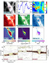 |
Fig. 2. Example of our multi-wavelength quality assurance scoring for candidate H I holes. Panels a–g: Each panel corresponds to the same hole (Hole 1) with the red ellipse marking its boundary and annotations in light blue giving the score for each feature. (a) H I moment-0 map showing a cavity. (b) H I line profile along the blue dashed line in panel a, used to quantify a 50% surface brightness depression. (c) H I velocity-dispersion (moment-2) map highlighting locally elevated σHI. (d1–d3) Individual H I channel map at representative velocities; the hole is visible in > 4 consecutive channels. (e) GALEX FUV map with bright emission coincident with the hole. (f) Hα emission map with strong flux within the hole. (g) Hα velocity-dispersion map with elevated σHα inside the hole. Bottom row: Position–velocity (PV) diagrams illustrating the three morphological classes of holes following Brinks & Bajaja (1986). The PV panels here (left to right) show Hole 3 (Type I), Hole 2 (Type II), and Hole 1 (Type III). Hole 2 also suffers from a tidal interaction, see Section 4. |
3.3.2. Derived properties
The derived properties are as follows. Most of the following equations, if not specifically cited, are adopted from the past H I hole studies conducted by Bagetakos et al. (2011) and Pokhrel et al. (2020):
-
Diameter,
 .
. -
The galactocentric distance in pc of a hole with centre (α, δ) to the galaxy centre (α0, δ0) in radians, can be obtained using the distance to the galaxy (D) in pc, position angle (θ), and inclination (i):
 (1)
(1) -
The kinetic age in Myr can be calculated from the diameter in parsec and the expansion velocity in km s−1,
 (2)
(2) -
H I column density,
![Mathematical equation: $$ \begin{aligned} N_{\rm HI} = 1.823 \times 10^{18} \sum _i \left[ \frac{S^i_{\rm avg}}{1.66\times 10^{-3} B_{\rm maj} B_{\rm min}} .\Delta v \right]. \end{aligned} $$](/articles/aa/full_html/2025/11/aa56351-25/aa56351-25-eq4.gif) (3)
(3)Here, Savgi is the mean H I flux density around the hole in mJy/beam, in each velocity channel i. Bmaj and Bmin are beam sizes in arcsec, Δv channel width in km s−1.
-
The effective thickness, ℓ(r), of the atomic hydrogen disk is calculated from the inclination of the galaxy, i, as:
![Mathematical equation: $$ \begin{aligned} \ell (r) [\mathrm{pc} ] = \frac{Z_0 \sqrt{2\pi }}{\cos i}\cdot \end{aligned} $$](/articles/aa/full_html/2025/11/aa56351-25/aa56351-25-eq5.gif) (4)
(4)Here, the scale height Z0 is derived from the H I velocity dispersion (≈12 km s−1), assuming hydrostatic equilibrium of the atomic gas in the gravitational potential of the stellar disk, with negligible dark matter (Combes & Becquaert 1997):
![Mathematical equation: $$ \begin{aligned} Z_0 [\mathrm{pc} ]&= \frac{v_\mathrm{disp} }{\sqrt{4\pi G \rho (r)}},\end{aligned} $$](/articles/aa/full_html/2025/11/aa56351-25/aa56351-25-eq6.gif) (5)
(5) (6)
(6)is the volumic stellar density, Σ*(r) the stellar surface density, re* the stellar exponential radial scale and hz* is the constant scale height of stellar disks (e.g. Bottema 1993). We adopted the stellar exponential radial scale from Casasola et al. (2017), which utilised the IRAC data to calculate the stellar scale length of M101 to be 2.09 arcmin ≈ 3.89 kpc. We deduced Σ0* to be 381 M⊙ pc−2 from their study. We also considered hz* = re/7.3 ≈ 0.53 kpc following Leroy et al. (2008), who adopted the average flattening ratio of 7.3 from Kregel et al. (2002). This is based on the assumption that the height of the stellar disk is independent of its radius (van der Kruit & Searle 1982).
-
The energy required to power the hole can be calculated using two different formulae. First, using Chevalier (1974), which is more dependent on the diameter of the hole, and the second using McCray & Kafatos (1987), which has high dependence on the expansion velocity.
![Mathematical equation: $$ \begin{aligned} E_{\mathrm{Ch} } [\mathrm{erg} ]&= 5.3 \times 10^{43} n_0^{1.12}[\mathrm{cm} ^{-3}] \left(\frac{d [\mathrm{pc} ]}{2} \right)^{3.12} v_{\mathrm{exp} }^{1.4} [\mathrm{km s} ^{-1}] , \end{aligned} $$](/articles/aa/full_html/2025/11/aa56351-25/aa56351-25-eq8.gif) (7)
(7)![Mathematical equation: $$ \begin{aligned} E_{\mathrm{Mc} }[\mathrm{erg} ]&= n_0 \left(\frac{d[\mathrm{pc} ]}{194}\right)^2 \left(\frac{v_\mathrm{exp} }{5.7} \right)^3 \times 10^{51}. \end{aligned} $$](/articles/aa/full_html/2025/11/aa56351-25/aa56351-25-eq9.gif) (8)
(8)Here we took the density of the ambient medium, n0, as the particle density of the atomic hydrogen, nHI, by ignoring contributions from He and H2. The midplane H I volume density (nHI) is calculated using the column density as follows:
 (9)
(9) -
H I mass of the hole:
![Mathematical equation: $$ \begin{aligned} M_\mathrm{HI} [\mathrm{M} _\odot ] = 0.0245 n_\mathrm{HI} V, \end{aligned} $$](/articles/aa/full_html/2025/11/aa56351-25/aa56351-25-eq11.gif) (10)
(10)where the volume of the hole is given by
![Mathematical equation: $$ \begin{aligned} V [\mathrm{pc}^3] = \frac{4}{3}\pi \left(\frac{d}{2} \right)^3. \end{aligned} $$](/articles/aa/full_html/2025/11/aa56351-25/aa56351-25-eq12.gif) (11)
(11)
4. Results
Out of the 72 H I holes surveyed (52 from K93 plus 20 newly identified cavities), nine satisfed our quality threshold (Q ≥ 15) and exhibit the most compelling multi-wavelength signatures of galactic fountains. Figure 3 maps these nine high-confidence sites onto the H I moment-0 image of M101 as red ellipses. Four of the 52 ‘classic’ K93 holes (dashed, red ellipses) and five of the new bubbles (solid, red ellipses) pass our scoring cut, while holes with intermediate scores (10 < Q < 15) are shown in purple for completeness.
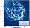 |
Fig. 3. H I moment-0 map of NGC 5457 (M101), overlaid with the locations of highly likely sites of galactic fountains. Regions are categorized based on quality flags (Q): red dashed ellipses mark holes from K93 with Q ≥ 15, red solid ellipses show newly identified holes with Q ≥ 15, purple dashed ellipses correspond to K93 holes with 10 < Q < 15, and purple solid ellipses mark new detections with 10 < Q < 15. The background blue-scale image shows the integrated H I emission, with brightness scaled between the 10th and 98th percentiles. The nine regions in red are the identified sites of galactic fountains. |
Tables 3 and 4 list the observed and derived properties of these nine holes, respectively. Briefly, their diameters span 0.5 − 2.4 kpc (median 0.7 kpc), expansion velocities run from 7 to 54 km s−1 (median 10 km s−1), and kinetic ages range from 18 to 93 Myr (median ∼ 31 Myr). The implied H I masses displaced were 1 × 10⁷ − 2 × 10⁹ M⊙ (median: 1.5 × 10⁸ M⊙), and the required energies (via Chevalier’s formula) lie between 1053 and 1056 erg (median: 3.5 × 1054 erg). These best-score holes tend to coincide with prominent spiral-arm H II complexes (e.g. NGC 5461, 5462, 5455), confirming that fountain-driving feedback is concentrated in the disk’s active star-forming regions.
Physical properties observed in the nine H I holes that are sites hosting galactic fountains.
Derived properties of the nine H I holes that are sites hosting galactic fountains.
Our two discovery routes yield a complementary population. The four largest cavities (diameters 1.6–2.4 kpc; Figure 4) were all catalogued by K93. In contrast, the five smaller holes (0.5–0.7 kpc; Figure A.1) emerged only from our SITELLE-first approach. This hierarchy of scales demonstrates that high-resolution multi-wavelength data can reveal more modest but still fountain-driven structures that previous H I surveys missed. For these smaller bubbles, we could not reliably assign Brinks types via PV diagrams; instead, we adopted the local H I velocity dispersion as an upper limit on the expansion speed.
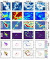 |
Fig. 4. Multi-wavelength views of the four biggest sites of galactic fountains in M101 marked by red ellipses. From top: H I velocity map overlayed with its 5th and 95th flux contours in black; H I velocity dispersion; FUV flux map; Hα flux map; Hα velocity dispersion map; the ratio of [S II] to Hα flux overlayed with the positions of optically identified SNRs by Matonick & Fesen (1997) in black symbols. |
Hole 3 is the largest cavity (2.4 kpc diameter) and also the oldest (∼93 Myr), located on the south-eastern arm adjacent to NGC 5461. Its PV diagram shows a fully “blown-out” type I signature, with no coherent shell walls (vexp ≲ 13 km s−1). The lack of interior Hα or FUV emission is consistent with its advanced age (the progenitor OB stars appear to have died). The filamentary clumps at its rim and a two-component fit to the Hα line (whose centroid separation matches vexp), point to triggered star formation along the shell edge. This is also adjacent to where the 2023 SN went off.
Hole 1 is the second largest cavity (2.03 kpc diameter) and the largest expansion velocity of 54 km s−1. It was already discovered by Kamphuis et al. (1991) as the first clear case of an expanding H I shell associated to an H I hole, corresponding to the energy of a thousand SNe. Situated on the north-eastern arm, Hole 2 exhibits the second largest expansion velocities, ∼40 km s−1, and was one of the holes inferred from both approaches. Although bubble morphology is evident on the rim of this hole with SITELLE RGB, the Hα line does not decompose cleanly into two components, suggesting geometric projection effects or rapid shell fragmentation at this evolutionary stage. Considering the exceptionally high velocity dispersion in this hole (cf second row and second column in Figure 4, and the middle panel in bottom row of Fig. 2), it is possible that this hole is suffering in addition from a tidal interaction from the M101 dwarf companion NGC 5477, as proposed by Combes (1991), or a collision with a large extra-galactic gas cloud as proposed by van der Hulst & Sancisi (1988), since it corresponds exactly to the perturbed region.
Among the small bubbles, Hole 6 stands out as the sole H I cavity that coincides precisely with an optical rim (Figure A.1). With a diameter of just 0.6 kpc, it shows elevated velocity dispersion in both H I moment-2 and Hασ maps at its core, and hosts a compact FUV cluster at its centre.
5. Discussion
5.1. 20 New H I holes
Approach 2 yields 20 new and smaller holes that were missed by the 15″ resolution of the K93 studies. Here, we discuss their size distribution, age, and shape using Figure 5. The new holes peaked at smaller radii (150–400 pc), whereas the original sample is biased towards radii ≥ 400 pc. This size-distribution shift directly reflects the factor-of-2 improvement in spatial resolution from THINGS (6″) versus the earlier 15″ WSRT data and demonstrates how higher resolution reveals a hierarchy of feedback structures.
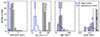 |
Fig. 5. Comparison of properties between the 20 new H I holes in blue and the 52 K93 holes in grey. The medians of each sample are plotted as dashed lines. As expected, the new holes span smaller diameters and are younger than those of the K93 sample. However, these younger holes do not seem to have a more circular shape than the older ones. |
These new holes expand at only 5–17 km s−1, far slower than the 25–45 km−1 typical of the K93 sample. Because the PV diagrams of sub-kpc cavities rarely show distinct approaching or receding bumps, we estimate each small hole’s expansion velocity simply as the H I moment-2 dispersion averaged over its area. This procedure naturally yields a lower vexp than for the K93 holes, due to the measurement method: tiny shells cannot be kinematically resolved as well as 1 kpc-scale bubbles. Consequently, when we computed the tkin (as we did for the high Q sites), they appeared systematically similar in age (median ∼ 30 Myr) to their larger, faster K93 holes (∼35 Myr). This is clear from Figure 6, which confirms that we have an observational bias of lower velocities for the newly identified holes. We note that the error bars on vexp for these small holes are much larger, since the estimated expansion velocity is very close to the H I typical velocity dispersion of 10 km s−1. These large relative errors of up to ∼100% prevent us from estimating their corresponding energy with precision.
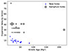 |
Fig. 6. Expansion velocities of the new and old holes plotted against their kinetic age. The size of any symbol is proportional to the diameter of the H I hole it represents. Even if their sizes are bigger, the relatively higher expansion velocities of the K93 sample holes push them to lie within a younger age area of the plot. The slower expansion velocities, close to the local H I velocity dispersion (∼10 km s−1), render the kinetic age of the new sample very similar to that of the old. |
Both samples show a wide range of axial ratios (0.4–1.0). Ideally, we expected that the differential rotation would shear holes into an elliptical shape with time. This would also mean that the shape of the bigger holes of the K93 sample should be more elliptical than the younger ones found in this work. Consequently, we compared the axial ratio and kinetic age of holes (Figure 7) and found no statistically significant correlation. This lack of correlation might be due to the low shear in the rotation curve of this late-type galaxy, with a very light bulge. The rotation is almost a solid-body one until a radius of 10 kpc (Bosma et al. 1981).
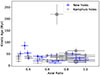 |
Fig. 7. Kinetic age vs axial ratio of the new (blue) and old (grey) holes, with the size of the symbols being representative of the hole diameter. This denotes a very weak negative correlation between axial ratio and kinetic age in our sample. This statistically insignificant relationship confirms that one cannot correlate the shape of the holes to its age. |
We also examined of these newly found holes as a function of the radius from the centre of the galaxy. There is a weak trend suggesting that the age of the H I hole increases with galactocentric distance. This indicates that inner-disk shells are, on average, younger, consistent with more rapid dissolution in regions of denser gas. However, the scatter is large, and the trend is not yet robust, as shown in Figure 8.
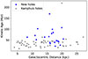 |
Fig. 8. Variation of age with galactocentric distance. The Pearson r value = 0.2 with a p-value of 0.08. This indicates a weak positive linear correlation between age and galactocentric distance. In other words, as galactocentric distance increases, age tends to increase slightly, but the relationship is not strong. |
If we assume that all of these holes were indeed powered by type II SNe, we can plot their “expansion” velocities (which in our case is an upper limit) against their diameters as done in Figure 9 and reversely use Eq. (7) to determine the energy required to power them. We take the n0 value to be 0.35 cm−3, which is the midplane density discussed by Kuntz et al. (2003). The following equation is based on the hydrodynamical description of the evolution of SNe modelled by Chevalier (1974), where they related the time with the radius (R) of the holes and expansion velocity vexp to be:
![Mathematical equation: $$ \begin{aligned} t [\mathrm{Myr}] = 0.304R/v_\mathrm{exp} . \end{aligned} $$](/articles/aa/full_html/2025/11/aa56351-25/aa56351-25-eq13.gif) (12)
(12)
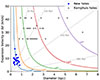 |
Fig. 9. Upper limits of the expansion velocity (given by the average velocity dispersion inside the hole) vs their diameters. The coloured curves are traced assuming the holes are powered by SNe, with total energy labelled on each curve. The dashed grey lines correspond to different ages (see text). |
We use this to draw constant time and energy lines on Figure 9 as was done by Puche et al. (1992) for the nearby dwarf galaxy Holmberg II. As in their case, this equation gives ages 3 times lower than the kinetic ages we calculate. Furthermore, it is important to note here that theseestimates of energy are not necessarily related to the energy estimated in Table 4 to power the four largest fountain-sites.
As a final step, we study the radial trends of the distribution of both the new and old H I holes in the galaxy as opposed to the SFR. Figure 10 compares the radial surface density of H I holes to the dust-corrected FUV SFR profile (Refer to Appendix A for FUV-derived SFR calculation). We found a moderate anti-correlation (r = −0.57, p = 0.017) between SFR surface density, ΣSFR(R) and surface density of the H I holes. Regions with the highest ongoing star formation (inner 3–5 kpc) surprisingly host fewer large H I cavities, perhaps because vigorous feedback has already disrupted old shells or because high SFR goes hand in hand with high gas density, which can either refill the holes more rapidly or stall hole expansion before large cavities develop. This apparent deficit could also reflect a detection bias, since feedback-driven holes near galaxy centres are more difficult to distinguish from the underlying lack of atomic gas in regions dominated by molecular gas. Beyond 5 kpc, the number of holes rises as the SFR surface density tails off, suggesting that past episodes of clustered SNe have carved long-lasting cavities in the outer disk.
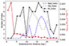 |
Fig. 10. Radial distribution of H I-hole counts compared to FUV-derived, dust-corrected star-formation-rate surface density. The two profiles exhibit a statistically significant moderate anti-correlation (Pearson r = −0.57, p = 0.017), indicating that regions of elevated recent star formation tend to host fewer H I holes. |
We noted that several new H I holes rarely coincided with the bubble feature visible in SITELLE RGB imagery. This might be due to the different time scales involved, and also to the previous star formation site and consequent SNe having triggered new star formation in the adjacent region. Another simpler explanation would be the fact that the part of the disk that pushed away the neutral gas (thereby creating cavities) has now moved due to the rotational motion.
5.2. Fountains in face-on galaxies
The combination of shell morphology, stellar associations, and kinematic evidence builds a compelling case that stellar feedback is responsible for carving these cavities in M101’s neutral gaseous disk. Comparing this to the edge-on galaxies where one usually detects extraplanar gas or line-of-sight lagging halos as evidence of fountain flows (e.g. Rand 1998), here we see the imprints of those flows on the disk and the launch sites of the fountains. This proves that studying face-on galaxies offers a complementary perspective.
All nine high-quality fountain candidates coincide with regions of recent star formation. In each case, we detected Hα emission within the cavity or along its rim. The former case indicates that the hole is formed in the last few Myrs and the responsible stars are still alive. In the latter case, where Hα is rim-dominant, they are almost always coincident with FUV emissions in the centre. From this, we infer that the hole was created hundreds of Myr ago: the ionising population has aged, yet secondary ‘contagious’ star formation along the compressed shell continues to power localised Hα along the rims. In every fountain site, the previous generation of stars has successfully displaced the neutral gas, revealing clear depressions in H I moment-zero map, accompanied by elevated velocity dispersion in both H I and Hα (moment-2).
Re-examining Figure 4, the four largest cavities exhibit classical super-shell or super-bubble morphologies. Two of these (leftmost and rightmost panels) were previously classified as a super-bubble and a super-shell by Kamphuis et al. (1991) and Chakraborti & Ray (2011), respectively. Their implied energy requirements ∼1056 − 57 erg exceed by two orders of magnitude the budget of our smaller fountain sites.
Matonick & Fesen (1997) carried out an optical survey of M101 and catalogued 93 SNRs, classifying their morphologies as stellar, filled, diffuse, arc or shell. When we overlaid their positions on the [S II]/Hα map (bottom panel of Figs. 4 and A.1), five of our nine high-quality fountain candidates lie within a few hundred parsecs of these SNRs. In particular, Holes 1 and 3 are delineated by multiple remnants, and additionally, several of our intermediate Q-score detections (purple ellipses) also coincide with SNRs along their rims.
The multi-wavelength dataset of these nine sites does not show any strong evidence of inflowing gas. However, we can deduce that from other observations of edge-on galaxies, where we see gas above the disk, and also from the amplitude of the expansion velocity, which is far below the escape velocity estimated to be 240 km s−1 (Kuntz et al. 2003), the gas expelled by the SNe (at median velocities of 34.5 km s−1) must return to the disk. To more precise the maximum height at which the H I gas can be expelled, and the time-scale of its travel outside the plane, we have computed these quantities, from vexp and the restoring force from the stellar disk, in Table 5. This gives an order of the magnitude of the feedback efficiency when the gas is unavailable for star formation.
Properties of the nine galactic fountains.
5.3. Mechanical energy
All of the mechanical energy imparted to the ISM comes from OB stars via ionising photons, stellar winds or SNe explosions (Abbott 1982; McCray & Kafatos 1987; Agertz et al. 2013; Kim & Ostriker 2015).
Of the two energy estimates in this study, we have shown in Table 4 that both equations from Chevalier (1974) and McCray & Kafatos (1987) give comparable results, despite their different sensitivity to expansion velocities and diameters. It is possible to use these estimates to calculate the number of SNe that produced these features. According to the formula by McCray & Kafatos (1987), the radius of an H I shell is given by:
![Mathematical equation: $$ \begin{aligned} R_s \mathrm{[pc]}&= 97 \left(\frac{N_{*} E_{51}}{n_0}\right)^{1/5} t_7^{3/5}, \end{aligned} $$](/articles/aa/full_html/2025/11/aa56351-25/aa56351-25-eq14.gif) (13)
(13)
 (14)
(14)
where N* is the number of SNe, t7 is the age of the shell in 107 years, E51 is the energy deposited by the SNe in units of 1051 erg and n0 is the density of the ambient interstellar medium in cm−3 which can be considered to be equal to nH as we did in Section 3.3.2. We found N* between 100 and 104, for the nine holes considered here in detail.
6. Conclusions
We have investigated galactic fountains in the almost face-on, spiral galaxy M101, comparing ionised, neutral gas and star clusters mapped through Hα, H I-21 cm and FUV. We use high-resolution data from THINGS for the H I emission, NGS-GALEX for UV, and SITELLE-SIGNALS IFU for the Hα tracer. The Hα gas is ionised by OB stars of a lifetime shorter than 10 Myr, and the FUV emission remains after 100 Myr, dating the last star-forming event. Supernovae explosions accompanying the star formation blow away the neutral gas, digging H I-holes in the galaxy plane, and sending material above the plane, which then infalls back to the plane like a fountain (Fraternali & Binney 2006, 2008). This delays star formation and plays a feedback role. We revisited the 52 H I holes catalogued by K93, and found 20 more holes, essentially in the outer parts of the galaxy. We have characterised the feedback processes and quantified their efficiency through measurements of sizes, ages, mechanical energies, and displaced gas masses. These 20 new holes are smaller in size and expansion velocity, mainly due to the increased spatial and velocity resolution. There is a deficit of small holes in the inner regions. This could be a selection bias, since small holes are easier to detect in the outer parts, where the gas density is lower, while in the inner parts, the small holes are more rapidly refilled or their expansion gets stalled. All H I hole properties, such as their size, axial ratio, their atomic gas column density and their kinetic energy, based on the expansion velocity vexp of the bubble, are studied as a function of their distance to the galaxy centre. There is no correlation between the axis ratio and the distance from the centre, maybe because this late-type galaxy has almost solid-body rotation until 10 kpc, meaning little shearing of the bubbles. Their age is estimated from their size and vexp, assumed constant during the bubble expansion. The energy of the bubble is computed from vexp, its diameter, and the volumic density of the gas n0 in which it expands, from two methods (Chevalier 1974; McCray & Kafatos 1987). We derive from these energies that the holes were created by several SNe between 100 and 104. We mapped in more detail the nine holes satisfying strong criteria to be a true fountain effect. Most of these holes contain FUV emission inside, and some Hα at their borders, or somewhat offset, indicating contagious star formation. Young stars and Hα are found inside only one small hole, showing that these are relatively rare. The largest hole of 2.4 kpc and the oldest age (94 Myr) has no Hα nor UV emission, and is consistent with an old fountain effect, when the star formation has terminated. Globally, the holes are relatively old, and it is difficult to find in their centre the very star formation at the origin of the hole. Therefore, no correlation can be found between the present star formation and the mechanical energy of the hole. The kinetic age of H I holes is remarkably constant with radius, around 50 Myr, and does not vary with size and vexp. The number of holes is smaller in the galaxy centre, where star formation is higher, which may look like a paradox, but is in fact a selection bias. It is more difficult to see H I holes where the gas is denser, and the rotation period is shorter, since holes are then smaller, and destroyed by star formation feedback. Finally, we note that some regions might also be perturbed by tidal interactions, as is likely for Hole 2, since M101 is highly perturbed, as is obvious from its remarkable lopsidedness.
Acknowledgments
AS would like to thank Laurent Drissen and Thomas Martin for their valuable help with analysing the SITELLE data. This work was supported by the Action Thématique Cosmology-Galaxies (ATCG) of the CNRS/INSU PN Astro. This research was based on observations obtained at the CFHT, which is operated from the summit of Mauna Kea by the National Research Council of Canada, the Institut National des Sciences de l’Univers of the Centre National de la Recherche Scientifique of France, and the University of Hawaii. The authors wish to recognise and acknowledge the very significant cultural role that the summit of Mauna Kea has always had within the indigenous Hawaiian community. The authors are most grateful to have the opportunity to conduct observations from this mountain. The observations were obtained with SITELLE, a joint project between Université Laval, ABB-Bomem, Université de Montréal, and the CFHT, with funding support from the Canada Foundation for Innovation (CFI), the National Sciences and Engineering Research Council of Canada (NSERC), Fonds de Recherche du Québec – Nature et Technologies (FRQNT), and CFHT. The collaboration is grateful to the FRQNT, CFHT, the Canada Research Chair program, the National Science foundation NSF – 2109124, Natural Sciences and Engineering Research Council of Canada NSERC – RGPIN-2023-03487, the Swedish Research Council, the Swedish National Space Board, the Royal Society, and the Newton Fund via the award of a Royal Society-Newton Advanced Fellowship (NAF\R1\180403), FAPESC, CNPq, FAPESP (2014/11156-4), FAPESB (7916/2015), and CONACyT (CB2015-254132).
References
- Abbott, D. C. 1982, ApJ, 263, 723 [NASA ADS] [CrossRef] [Google Scholar]
- Agertz, O., Kravtsov, A. V., Leitner, S. N., & Gnedin, N. Y. 2013, ApJ, 770, 25 [NASA ADS] [CrossRef] [Google Scholar]
- Armillotta, L., Fraternali, F., & Marinacci, F. 2016, MNRAS, 462, 4157 [NASA ADS] [CrossRef] [Google Scholar]
- Bagetakos, I., Brinks, E., Walter, F., et al. 2011, AJ, 141, 23 [NASA ADS] [CrossRef] [Google Scholar]
- Boomsma, R., Oosterloo, T. A., Fraternali, F., van der Hulst, J. M., & Sancisi, R. 2008, A&A, 490, 555 [NASA ADS] [CrossRef] [EDP Sciences] [Google Scholar]
- Bosma, A., Goss, W. M., & Allen, R. J. 1981, A&A, 93, 106 [NASA ADS] [Google Scholar]
- Bottema, R. 1993, A&A, 275, 16 [NASA ADS] [Google Scholar]
- Bregman, J. N. 1980, ApJ, 236, 577 [NASA ADS] [CrossRef] [Google Scholar]
- Brinks, E., & Bajaja, E. 1986, A&A, 169, 14 [NASA ADS] [Google Scholar]
- Camps-Fariña, A., Zaragoza-Cardiel, J., Beckman, J. E., et al. 2017, MNRAS, 468, 4134 [CrossRef] [Google Scholar]
- Casasola, V., Cassarà, L. P., Bianchi, S., et al. 2017, A&A, 605, A18 [NASA ADS] [CrossRef] [EDP Sciences] [Google Scholar]
- Chakraborti, S., & Ray, A. 2011, ApJ, 728, 24 [Google Scholar]
- Chevalier, R. A. 1974, ApJ, 188, 501 [Google Scholar]
- Combes, F. 1991, A&A, 243, 109 [NASA ADS] [Google Scholar]
- Combes, F., & Becquaert, J. F. 1997, A&A, 326, 554 [NASA ADS] [Google Scholar]
- Comrie, A., Wang, K. S., Hsu, S. C., et al. 2021, Astrophysics Source Code Library [record ascl:2103.031] [Google Scholar]
- Davies, R. D. 1975, MNRAS, 170, 45 [Google Scholar]
- Deul, E. R., & den Hartog, R. H. 1990, A&A, 229, 362 [NASA ADS] [Google Scholar]
- Drissen, L., Martin, T., Rousseau-Nepton, L., et al. 2019, MNRAS, 485, 3930 [NASA ADS] [CrossRef] [Google Scholar]
- Egorov, O. V., Kreckel, K., Glover, S. C. O., et al. 2023, A&A, 678, A153 [NASA ADS] [CrossRef] [EDP Sciences] [Google Scholar]
- Fraternali, F., & Binney, J. J. 2006, MNRAS, 366, 449 [CrossRef] [Google Scholar]
- Fraternali, F., & Binney, J. J. 2008, MNRAS, 386, 935 [CrossRef] [Google Scholar]
- Fraternali, F., van Moorsel, G., Sancisi, R., & Oosterloo, T. 2002, AJ, 123, 3124 [CrossRef] [Google Scholar]
- Ginsburg, A., Robitaille, T., & Beaumont, C. 2016, Astrophysics Source Code Library [record ascl:1608.010] [Google Scholar]
- Hao, C.-N., Kennicutt, R. C., Johnson, B. D., et al. 2011, ApJ, 741, 124 [Google Scholar]
- Heiles, C. 1979, ApJ, 229, 533 [NASA ADS] [CrossRef] [Google Scholar]
- Heiles, C. 1984, ApJS, 55, 585 [NASA ADS] [CrossRef] [Google Scholar]
- Houck, J. C., & Bregman, J. N. 1990, ApJ, 352, 506 [Google Scholar]
- Hu, E. M. 1981, ApJ, 248, 119 [NASA ADS] [CrossRef] [Google Scholar]
- Kamphuis, J. J. 1993, Ph.D. Thesis, University of Groningen, Netherlands [Google Scholar]
- Kamphuis, J., & Briggs, F. 1992, A&A, 253, 335 [NASA ADS] [Google Scholar]
- Kamphuis, J., Sancisi, R., & van der Hulst, T. 1991, A&A, 244, L29 [Google Scholar]
- Keel, W. C., Holberg, J. B., & Treuthardt, P. M. 2004, AJ, 128, 211 [Google Scholar]
- Kim, C.-G., & Ostriker, E. C. 2015, ApJ, 802, 99 [NASA ADS] [CrossRef] [Google Scholar]
- Kregel, M., van der Kruit, P. C., & de Grijs, R. 2002, MNRAS, 334, 646 [NASA ADS] [CrossRef] [Google Scholar]
- Kuntz, K. D., Snowden, S. L., Pence, W. D., & Mukai, K. 2003, ApJ, 588, 264 [Google Scholar]
- Lara-López, M. A., Pilyugin, L. S., Zaragoza-Cardiel, J., et al. 2023, A&A, 669, A25 [NASA ADS] [CrossRef] [EDP Sciences] [Google Scholar]
- Leroy, A. K., Walter, F., Brinks, E., et al. 2008, AJ, 136, 2782 [Google Scholar]
- Leroy, A. K., Walter, F., Sandstrom, K., et al. 2013, AJ, 146, 19 [Google Scholar]
- Martin, D. C., Fanson, J., Schiminovich, D., et al. 2005, ApJ, 619, L1 [Google Scholar]
- Martin, T., Drissen, L., & Joncas, G. 2015, ASP Conf. Ser., 495, 327 [Google Scholar]
- Martin, T. B., Prunet, S., & Drissen, L. 2016, MNRAS, 463, 4223 [Google Scholar]
- Matonick, D. M., & Fesen, R. A. 1997, ApJS, 112, 49 [NASA ADS] [CrossRef] [Google Scholar]
- McCray, R., & Kafatos, M. 1987, ApJ, 317, 190 [NASA ADS] [CrossRef] [Google Scholar]
- Morisset, C. 2018, https://doi.org/10.5281/zenodo.1206115 [Google Scholar]
- Oosterloo, T., Fraternali, F., & Sancisi, R. 2007, AJ, 134, 1019 [Google Scholar]
- Pokhrel, N. R., Simpson, C. E., & Bagetakos, I. 2020, AJ, 160, 66 [NASA ADS] [CrossRef] [Google Scholar]
- Puche, D., Westpfahl, D., Brinks, E., & Roy, J.-R. 1992, AJ, 103, 1841 [Google Scholar]
- Putman, M. E., Peek, J. E. G., & Joung, M. R. 2012, ARA&A, 50, 491 [Google Scholar]
- Rampazzo, R., Mazzei, P., Marino, A., et al. 2022, A&A, 664, A192 [NASA ADS] [CrossRef] [EDP Sciences] [Google Scholar]
- Rand, R. J. 1998, PASA, 15, 106 [Google Scholar]
- Rousseau-Nepton, L., Martin, R. P., Robert, C., et al. 2019, MNRAS, 489, 5530 [NASA ADS] [CrossRef] [Google Scholar]
- Rupke, D. S. N. 2018, Galaxies, 6, 138 [Google Scholar]
- Schruba, A., Leroy, A. K., Walter, F., et al. 2011, AJ, 142, 37 [NASA ADS] [CrossRef] [Google Scholar]
- Shapiro, P. R., & Field, G. B. 1976, ApJ, 205, 762 [NASA ADS] [CrossRef] [Google Scholar]
- Shappee, B. J., & Stanek, K. Z. 2011, ApJ, 733, 124 [NASA ADS] [CrossRef] [Google Scholar]
- Somerville, R. S., & Davé, R. 2015, ARA&A, 53, 51 [Google Scholar]
- Tody, D. 1986, SPIE Conf. Ser., 627, 733 [Google Scholar]
- van der Hulst, T., & Sancisi, R. 1988, AJ, 95, 1354 [Google Scholar]
- van der Kruit, P. C., & Searle, L. 1982, A&A, 110, 61 [NASA ADS] [Google Scholar]
- van Woerden, H., Peletier, R. F., Schwarz, U. J., Wakker, B. P., & Kalberla, P. M. W. 1999, ASP Conf. Ser., 166, 1 [Google Scholar]
- Walter, F., Brinks, E., de Blok, W. J. G., et al. 2008, AJ, 136, 2563 [Google Scholar]
- Watkins, E. J., Kreckel, K., Groves, B., et al. 2023a, A&A, 676, A67 [NASA ADS] [CrossRef] [EDP Sciences] [Google Scholar]
- Watkins, E. J., Barnes, A. T., Henny, K., et al. 2023b, ApJ, 944, L24 [NASA ADS] [CrossRef] [Google Scholar]
- Westmeier, T., Braun, R., Brüns, C., Kerp, J., & Thilker, D. A. 2007, New Astron. Rev., 51, 108 [Google Scholar]
- Wilcots, E. M., & Miller, B. W. 1998, AJ, 116, 2363 [Google Scholar]
Appendix A: SFR calculation using GALEX data
We use the intensity (fd(nd)-int), sky-background (fd(nd)-skybg) and weight (fd(nd)-wt) from the GALEX data products to calculate the radial distribution of SFR of M101. The intensity and the sky-background maps are in units of counts per pixel, while the weight maps are dimensionless. The higher the weight of a pixel, the more confident we are in its intensity value.
The flux measurements have been made from the background-subtracted versions of the intensity images, whose units are in counts per second (CPS) by multiplying with a factor of 1.40 × 10¹⁵ for FUV. This gives the flux, Fν, in erg s−1 cm−2 Å−1. The FUV luminosity is obtained by:
![Mathematical equation: $$ \begin{aligned} L_\nu [\mathrm {erg\ s}^{-1} ] = 4\pi D_L^2 F_\nu \nu , \end{aligned} $$](/articles/aa/full_html/2025/11/aa56351-25/aa56351-25-eq16.gif) (A.1)
(A.1)
where DL is the luminosity distance to galaxy M101 in cm, ν = 442 is the FUV bandwidth. This luminosity needs to be corrected for dust attenuation, for which we must first calculate the FUV and NUV magnitudes using the background-subtracted intensity in counts per second, I:
 (A.2)
(A.2)
 (A.3)
(A.3)
The attenuation in FUV is thus obtained by using the following formula from Hao et al. (2011):
![Mathematical equation: $$ \begin{aligned} A_\mathrm{FUV} = 3.83 \left[ ( m_\mathrm{FUV} - m_\mathrm{NUV} ) - 0.022 \right]. \end{aligned} $$](/articles/aa/full_html/2025/11/aa56351-25/aa56351-25-eq19.gif) (A.4)
(A.4)
The luminosity is then corrected using:
 (A.5)
(A.5)
To obtain the dust-corrected SFR from the FUV luminosity, we calculate :
![Mathematical equation: $$ \begin{aligned} \mathrm{SFR} ^\mathrm{corr} _\mathrm{FUV} [M_\odot \mathrm{yr} ^{-1}]= \frac{L^\mathrm{corr} _\mathrm{FUV} }{10^{43.35}}. \end{aligned} $$](/articles/aa/full_html/2025/11/aa56351-25/aa56351-25-eq21.gif) (A.6)
(A.6)
All Tables
Physical properties observed in the nine H I holes that are sites hosting galactic fountains.
Derived properties of the nine H I holes that are sites hosting galactic fountains.
All Figures
|
Fig. 1. Multi-wavelength views of NGC 5457 or M101. Left: False-colour RGB composite of M101 using H I (THINGS, red), Hα (SITELLE, green), and FUV (GALEX, blue). The colour mapping is subtractive rather than additive, highlighting variations in neutral gas phase (H I), recently star-forming regions (Hα), and older star formation (FUV). Right: False-colour RGB composite of M101 using SITELLE’s SN1, SN2, and SN3 filters. The mosaic combines four pointings (each covering 11′×11′) to capture the full extent of the galaxy. |
| In the text | |
|
Fig. 2. Example of our multi-wavelength quality assurance scoring for candidate H I holes. Panels a–g: Each panel corresponds to the same hole (Hole 1) with the red ellipse marking its boundary and annotations in light blue giving the score for each feature. (a) H I moment-0 map showing a cavity. (b) H I line profile along the blue dashed line in panel a, used to quantify a 50% surface brightness depression. (c) H I velocity-dispersion (moment-2) map highlighting locally elevated σHI. (d1–d3) Individual H I channel map at representative velocities; the hole is visible in > 4 consecutive channels. (e) GALEX FUV map with bright emission coincident with the hole. (f) Hα emission map with strong flux within the hole. (g) Hα velocity-dispersion map with elevated σHα inside the hole. Bottom row: Position–velocity (PV) diagrams illustrating the three morphological classes of holes following Brinks & Bajaja (1986). The PV panels here (left to right) show Hole 3 (Type I), Hole 2 (Type II), and Hole 1 (Type III). Hole 2 also suffers from a tidal interaction, see Section 4. |
| In the text | |
|
Fig. 3. H I moment-0 map of NGC 5457 (M101), overlaid with the locations of highly likely sites of galactic fountains. Regions are categorized based on quality flags (Q): red dashed ellipses mark holes from K93 with Q ≥ 15, red solid ellipses show newly identified holes with Q ≥ 15, purple dashed ellipses correspond to K93 holes with 10 < Q < 15, and purple solid ellipses mark new detections with 10 < Q < 15. The background blue-scale image shows the integrated H I emission, with brightness scaled between the 10th and 98th percentiles. The nine regions in red are the identified sites of galactic fountains. |
| In the text | |
|
Fig. 4. Multi-wavelength views of the four biggest sites of galactic fountains in M101 marked by red ellipses. From top: H I velocity map overlayed with its 5th and 95th flux contours in black; H I velocity dispersion; FUV flux map; Hα flux map; Hα velocity dispersion map; the ratio of [S II] to Hα flux overlayed with the positions of optically identified SNRs by Matonick & Fesen (1997) in black symbols. |
| In the text | |
|
Fig. 5. Comparison of properties between the 20 new H I holes in blue and the 52 K93 holes in grey. The medians of each sample are plotted as dashed lines. As expected, the new holes span smaller diameters and are younger than those of the K93 sample. However, these younger holes do not seem to have a more circular shape than the older ones. |
| In the text | |
|
Fig. 6. Expansion velocities of the new and old holes plotted against their kinetic age. The size of any symbol is proportional to the diameter of the H I hole it represents. Even if their sizes are bigger, the relatively higher expansion velocities of the K93 sample holes push them to lie within a younger age area of the plot. The slower expansion velocities, close to the local H I velocity dispersion (∼10 km s−1), render the kinetic age of the new sample very similar to that of the old. |
| In the text | |
|
Fig. 7. Kinetic age vs axial ratio of the new (blue) and old (grey) holes, with the size of the symbols being representative of the hole diameter. This denotes a very weak negative correlation between axial ratio and kinetic age in our sample. This statistically insignificant relationship confirms that one cannot correlate the shape of the holes to its age. |
| In the text | |
|
Fig. 8. Variation of age with galactocentric distance. The Pearson r value = 0.2 with a p-value of 0.08. This indicates a weak positive linear correlation between age and galactocentric distance. In other words, as galactocentric distance increases, age tends to increase slightly, but the relationship is not strong. |
| In the text | |
|
Fig. 9. Upper limits of the expansion velocity (given by the average velocity dispersion inside the hole) vs their diameters. The coloured curves are traced assuming the holes are powered by SNe, with total energy labelled on each curve. The dashed grey lines correspond to different ages (see text). |
| In the text | |
|
Fig. 10. Radial distribution of H I-hole counts compared to FUV-derived, dust-corrected star-formation-rate surface density. The two profiles exhibit a statistically significant moderate anti-correlation (Pearson r = −0.57, p = 0.017), indicating that regions of elevated recent star formation tend to host fewer H I holes. |
| In the text | |
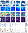 |
Fig. A.1. Same as Figure 4 for the smaller five sites of galactic fountains in M101. |
| In the text | |
Current usage metrics show cumulative count of Article Views (full-text article views including HTML views, PDF and ePub downloads, according to the available data) and Abstracts Views on Vision4Press platform.
Data correspond to usage on the plateform after 2015. The current usage metrics is available 48-96 hours after online publication and is updated daily on week days.
Initial download of the metrics may take a while.