| Issue |
A&A
Volume 703, November 2025
|
|
|---|---|---|
| Article Number | A152 | |
| Number of page(s) | 10 | |
| Section | The Sun and the Heliosphere | |
| DOI | https://doi.org/10.1051/0004-6361/202556401 | |
| Published online | 14 November 2025 | |
Image calibration between the Extreme Ultraviolet Imagers on Solar Orbiter and the Solar Dynamics Observatory
1
Institute of Physics, University of Graz, Universitätsplatz 5, 8010 Graz, Austria
2
High Altitude Observatory, National Center for Atmospheric Research, 3080 Center Green Dr, Boulder, USA
3
Kanzelhöhe Observatory for Solar and Environmental Research, University of Graz, Treffen am Ossiacher See, Austria
4
European Space Agency (ESA)-ECSAT, Fermi Avenue, Harwell, UK
5
Department of Physics, University of Oxford, Oxford, UK
6
Image Processing Laboratory (IPL) Department Universitat de València, València, Spain
7
Solar-Terrestrial Centre of Excellence (SIDC), Royal Observatory of Belgium, Ringlaan 3 Av. Circulaire, 1180 Brussels, Belgium
8
Trillium Technologies Inc. (Trillium USA), 8668 John Hickman Pkwy, STE 301 Frisco, TX, USA
⋆ Corresponding author: This email address is being protected from spambots. You need JavaScript enabled to view it.
Received:
14
July
2025
Accepted:
19
September
2025
Abstract
To study and monitor the Sun and its atmosphere, various space missions have been launched in the past decades. With rapid improvement in technology and different mission requirements, the data products are subject to constant change. However, for such long-term studies as solar variability or multi-instrument investigations, uniform data series are required. In this study, we built on and expanded the instrument-to-instrument translation (ITI) framework, which provides unpaired image translations. We applied the tool to data from the Extreme Ultraviolet Imager (EUI), specifically the Full Sun Imager (FSI) on Solar Orbiter and the Atmospheric Imaging Assembly (AIA) on the Solar Dynamics Observatory (SDO). This approach allowed us to create a homogeneous dataset that combines the two extreme ultraviolet (EUV) imagers in the 174/171 Å and 304 Å channels. We demonstrate that ITI is able to provide image calibration between Solar Orbiter and SDO EUV imagers, independent of the varying orbital position of Solar Orbiter. The comparison of the intercalibrated light curves derived from 174/171 Å and 304 Å filtergrams from EUI and AIA shows that ITI can provide uniform data series that outperform a standard baseline calibration. We evaluate the perceptual similarity in terms of the Fréchet inception distance, which demonstrates that ITI achieves a significant improvement of perceptual similarity between EUI and AIA. The study provides intercalibrated observations from Solar Orbiter/EUI/FSI with SDO/AIA, enabling a homogeneous dataset suitable for solar cycle studies and multi-viewpoint investigations.
Key words: telescopes / Sun: atmosphere / Sun: corona / Sun: heliosphere
© The Authors 2025
 Open Access article, published by EDP Sciences, under the terms of the Creative Commons Attribution License (https://creativecommons.org/licenses/by/4.0), which permits unrestricted use, distribution, and reproduction in any medium, provided the original work is properly cited.
This article is published in open access under the Subscribe to Open model. This email address is being protected from spambots. You need JavaScript enabled to view it. to support open access publication.
1. Introduction
The Solar Orbiter (Müller et al. 2020) mission, launched in 2020, has already provided exceptional insight into the study of solar flares, coronal mass ejections (CMEs), coronal holes, and very small brightenings with imagers in the extreme ultraviolet (EUV) and X-ray (e.g., Collier et al. 2024; Chitta et al. 2023; Berghmans et al. 2021; Schwanitz et al. 2023; O’Kane et al. 2021; Purkhart et al. 2024; Podladchikova et al. 2024; Saqri et al. 2024). In particular, the Extreme Ultraviolet Imager (EUI; Rochus et al. 2020) observes the solar atmosphere in the EUV, both globally and at high spatial and temporal resolution. With its highly elliptical orbit and the out-of-ecliptic transition in 2025, Solar Orbiter provides the perfect conditions to analyze eruptive phenomena from different vantage points. On the other hand, the Solar Dynamics Observatory (SDO; Pesnell et al. 2012) launched in a geosynchronous orbit around Earth in 2010 provides a long database of solar observations. In particular, with its high temporal and spatial resolution imaging capabilities from the Atmospheric Imaging Assembly (AIA; Lemen et al. 2012), SDO provides detailed insights into dynamic phenomena such as solar flares.
Long-term solar monitoring is important to understand solar activity and consequently solar eruptive events, as these pose a significant threat not only to Earth and its environment but also to our assets in space. The sunspot number forms the longest directly observed index for solar cycle and variability studies (Usoskin & Mursula 2003). On the other hand, the solar EUV radiation drives the variability in Earth’s upper atmosphere, affecting satellites, communication, and navigation (Woods et al. 2012). As more space missions are launched, we improve our understanding of the Sun’s atmosphere and therefore its eruptive phenomena. However, with rapid improvement in technology and also different mission requirements, the instruments and therefore the data products are changing. The calibration of these instruments ensures a direct intensity comparison, reducing the potential for bias caused by differences in instrumentation and also changes due to degradations in space. For multi-instrument solar cycle studies and long-term solar monitoring, uniform data series are required. Furthermore, the lifetime of these space missions is limited. Consequently, image calibration bridges the gap between older and newer missions to build a uniform data series.
Traditional image calibration methods for EUV observations are based on standardization by subtracting the average logarithmic intensity and dividing by the standard deviation of the logarithmic intensity in these observations, as shown by Hamada et al. (2020). Dos Santos et al. (2021) first applied deep neural networks using convolutional neural networks (CNNs) for autocalibration, including instrument degradation correction of the AIA instrument. Previous studies have also used deep neural networks for image enhancement (Díaz Baso & Asensio Ramos 2018) and image denoising (Díaz Baso et al. 2019). Youn et al. (2025) applied generative adversarial networks (GANs) to synthesize the remaining AIA channels on Solar Orbiter in order to perform a differential emission measure (DEM) analysis.
In order to obtain joint data products of the EUV imagers on board Solar Orbiter and SDO, we applied the instrument-to-instrument (ITI) translation tool (Jarolim et al. 2025). The ITI tool has been shown to be a universally applicable for solar image data, allowing image enhancement, image calibration, and super-resolution observations. In addition, ITI has been applied to ground-based solar data to mitigate seeing effects from the Kanzelhoehe Solar Observatory (KSO; Pötzi et al. 2021) and to reconstruct high-resolution ground-based solar observations from the GREGOR telescope (Schirninger et al. 2024). Our aim is to achieve simultaneous image calibration and image enhancement by applying the ITI tool to translate EUV observations from the EUI instrument on Solar Orbiter into corresponding observations from SDO/AIA.
An important property of ITI is that it utilizes unpaired image-to-image translation, which requires neither a spatial nor temporal overlap between the two datasets. This is particularly important for the calibration between Solar Orbiter and SDO, due to the sparse set of aligned observations. In addition, differences in instrument resolution, wavelength range, filter characteristics, and quality are complex, and a calibration based on statistical quantities is typically insufficient (Hamada et al. 2020). The neural network learns the image distribution of the ground-truth reference dataset and therefore allows translation between two instruments. This provides joint data products, which can be used for detection methods, such as coronal hole detections (Caplan et al. 2016; Reiss et al. 2021; Jarolim et al. 2021), flare detections (Nisticó et al. 2017), and triangulation methods as shown by Aschwanden et al. (2008), or for obtaining a 3D representation of the Sun from multi-viewpoint observations using neural radiance fields (SuNeRF; Jarolim et al. 2024), where ITI was also already used.
In Sect. 2 we introduce the data used in this study as well as the preprocessing steps to achieve machine-learning-ready datasets. Section 3 provides an overview of the method. The results of the study are discussed in Sect. 4, including a quantitative comparison in Sect. 4.1, a qualitative comparison in Sect. 4.2, a comparison of translations for different distances of Solar Orbiter to the Sun in Sect. 4.3, and a multi-viewpoint application in Sect. 4.4. In Sect. 5 we present our conclusions from this study.
2. Data
In this study, we applied the ITI tool to EUV observations from the Solar Orbiter/EUI instrument and used observations from SDO/AIA as the calibration target for image calibration. The EUI instrument is equipped with two EUV imagers, the Full Sun Imager (FSI) taking full Sun observations, and the High Resolution Imager (HRIEUV) providing high-resolution observations of a smaller field of view (FOV) of (1 R⊙)2 at 1 AU and (0.28 R⊙)2 perihelion, respectively (Rochus et al. 2020). We performed calibration between the 174 Å and 304 Å filters of Solar Orbiter/EUI/FSI and the 171 Å and 304 Å filters of SDO/AIA. Note that the AIA 171 Å and the FSI 174 Å channels observe emission from different iron ions, with AIA 171 Å primarily sensitive to Fe IX and FSI 174 Å dominated by Fe X. Consequently, differences between the images from these two channels are expected due to their different temperature sensitivity.
2.1. FSI data
The FSI instrument provides full Sun observations in two wavelength channels, 174 Å and 304 Å. With an FOV of two solar diameters at perihelion, the full solar disk including the extended solar corona can be observed when the spacecraft is pointed at the solar limb. The angular resolution of the telescope is 10 arcsec. Since the orbit of Solar Orbiter is very elliptical, the spatial resolution of the observations changes according to the distance to the Sun. At perihelion, Solar Orbiter covers a smaller region on the Sun and consequently achieves the highest resolution observations. We consider all observations available from the perihelion at ∼0.3 AU to the aphelion at ∼1.1 AU. Therefore, we aimed to achieve an image calibration that would also account for the varying resolution, due to the change in orbital position. The data used in this work were obtained from Data Release 6 (Kraaikamp et al. 2023).
To obtain a machine-learning-ready dataset, we preprocessed the FSI data by cropping all observations to an FOV of 1.1 solar radii and scaled them to an image size of 1024 × 1024 pixels. Cropping the full Sun observations to 1.1 solar radii prevented the sampling of patches that are completely off-limb, since training was performed using image patches. Furthermore, the pixel values were mapped to an interval [ − 1, 1], using normalization between the minimum intensity value and 90% of the maximum intensity value of the entire training dataset. The FSI 174 Å and 304 Å channels showed significant degradation; therefore, we applied a degradation correction by estimating the quiet Sun region over the entire training set from January 2022 to May 2023 and fit the degradation as a first-order polynomial (cf. Jarolim et al. 2025). The fit parameters extracted from the linear fit were used to correct for the degradation of the entire dataset including data after 2023. Consequently, the linear fit served as a degradation approximation for later times. We used the linear fit to avoid filtering out solar cycle effects. The degradation and the linear fit to the data are shown in Fig. A.1. The FSI dataset spans from January 2022 to February 2023. We note that the Solar Orbiter mission conducts Solar Orbiter Observing Plans (SOOPs; Zouganelis et al. 2020). The SOOPs are designed to understand how the Sun generates and controls the heliosphere from a combined in situ and remote sensing perspective. However, this also affects other instruments on the spacecraft. For some SOOPs, the imagers are not pointed at the center of the solar disk. This leads to intensity enhancements in the FSI data. To account for this, we removed all off-pointing SOOP observations from our dataset.
2.2. AIA data
For the reference dataset, which is our calibration target, we utilized observations from SDO/AIA in the 171 Å and 304 Å filters. The SDO spacecraft operates in a geosynchronous orbit around Earth at approximately 1 AU. The AIA instrument provides high-resolution observations in the EUV, with a spatial resolution of 1.5 arcseconds and a temporal cadence of 12 seconds. AIA’s FOV spans 1.3 solar radii, capturing both the full solar disk and the surrounding solar corona. Additionally, AIA offers a substantial database with observations starting from 2010. For our dataset, we considered one observation per day, starting from May 2011 to April 2024. We performed a visual inspection of the dataset and removed invalid observations (i.e., eclipse times, cosmic particles, or instrument-malfunctioned observations). Additionally, observations containing flares were excluded and were not considered for image calibration. Analogous to the preprocessing of the FSI observations, the AIA data were preprocessed by cropping all observations to 1.1 solar radii and mapping the pixel values to an interval [ − 1, 1] using the minimum intensity value and 90% of the maximum intensity value of the entire training dataset. Furthermore, the observations are down-sampled from 4096 × 4096 pixels to a resolution of 1024 × 1024 pixels. Additionally, we corrected for the time-dependent degradation of the AIA instrument using the correction table according to Barnes (2020).
2.3. Datasets
In total, the FSI dataset consists of 3699 observations in the time span from January 2022 to February 2023 for the 174 Å and 304 Å filters, and 4607 observations from May 2011 to April 2024 for the AIA reference dataset in both 171 Å and 304 Å, respectively (see Table 1). For training we split the dataset into training and validation sets, using data from February to October for training and observations from November and December for validation. This temporal separation reduces the risk of overlap between training and validation samples, which can occur due to the strong similarity between temporally adjacent observations (Kim et al. 2019).
Number of observations of the dataset split into training, validation, and three different test sets.
For our evaluation, we prepared four test sets. The first test set consists of observations when Solar Orbiter was close to the Sun-Earth line within 0.8 degrees longitude. It covers the period from November 11, 2021, to November 14, 2021, and March 20, 2024, from 13:00 to 17:00 UT with a cadence of one hour. In this time frame, no off-pointing was performed for Solar Orbiter, and therefore it allows a direct comparison with the AIA observations that we use as “ground truth”. There is a small latitude difference of ∼2.9° on average between Solar Orbiter and SDO, making pixel-based metrics and intensity ratio images inappropriate for comparison. We refer to this dataset as test set 1 (Earth-aligned). The second test set is to compare how the distance of Solar Orbiter to the Sun affects the ITI translations, containing observations from 0.3 AU to 0.9 AU. It covers the time range from May 15, 2023, to May 28, 2023, and February 2024 to March 2024. We refer to this dataset as test set 2 (variable distance). The third test set consists of observations where Solar Orbiter is not in the Sun-Earth line but has an overlap in the FOV with SDO/AIA, to investigate whether ITI is capable of image calibration for multi-viewpoint studies. This test set covers the period from October 21, 2023, to October 24, 2023. This test set allows for a visually comparative assessment of our calibrations with the ground truth AIA observations. We refer to this dataset as test set 3 (multi-viewpoint). The separation angle of the two spacecraft in longitude across test set 3 spans from 40° to 33°, where Solar Orbiter is west in longitude from SDO. Test set 4 (light curve) was used to perform a statistical light curve analysis of our ITI translations and the baseline calibration. It covers the period from March 2023 to January 2025. All observations in the time frame of the test sets, including ten days before and after, were removed from the training and validation set.
3. Method
We used the ITI tool to calibrate the EUI/FSI instrument onboard Solar Orbiter with SDO/AIA. The tool was originally developed by Jarolim et al. (2025) and is provided as an open source framework1. Previously, ITI was applied to data from SDO, the Solar Optical Telescope (SOT; Tsuneta et al. 2008) on board Hinode, the Solar and Heliospheric Observatory (SOHO; Domingo et al. 1995) and the Solar Terrestrial Relations Observatory (STEREO; Driesman et al. 2008) to obtain image calibration, image enhancement, and super-resolution observations.
The ITI tool is based on GANs (Goodfellow et al. 2020) and uses unpaired image-to-image translation (Zhu et al. 2017). The standard GAN setup consists of two competing networks, a generator network and a discriminator network. The aim of the generator network is to synthesize images in the reference domain so that the discriminator can no longer distinguish between real and synthesized images. Compared to paired image translation (Isola et al. 2017), no spatial or temporal overlap of the two datasets is required. The generator network learns the distribution of the reference dataset by mapping images from a domain A to the reference domain B. The generator networks use a U-net architecture with down-sampling and up-sampling blocks and skip connections that help the network to use the information from the down-sampling steps (Ronneberger et al. 2015). The discriminator networks consist of three individual networks, each of which performs down-sampling steps. This allows optimization to be carried out at multiple resolution scales (Wang et al. 2018).
In total, two discriminators and two generators are used for training. One training cycle involves translation from one instrument of domain A to the reference instrument of domain B and back to domain A (A-B-A). In a second cycle, the same translation is performed, but from domain B to domain A and back to B (B-A-B). The last two training cycles involve identity mappings using generator AB to translate images from domain B to domain B (B-B) and vice versa for images of domain A using generator BA (A-A).
3.1. Baseline calibration
In order to evaluate the performance of our model, we compared our ITI calibrations to a baseline calibration. Here, we calculated the mean and standard deviation of the FSI and AIA observations over the training set to adjust the counts, given in dynamical number per second (DN/s) of FSI to AIA. For AIA, the mean and standard deviation were calculated over the time range May 2011 to April 2024, and for FSI from January 2022 to February 2023. These statistics were computed using the original intensity values (DN/s), without applying a logarithmic function. The baseline calibrated FSI observations are then calculated as
![Mathematical equation: $$ \begin{aligned} \text{ FSI}_{cal,i}=[(\text{ FSI}_i - \mu _{\text{ FSI}}) / \sigma _{\text{ FSI}}] * \sigma _{\text{ AIA}} + \mu _{\text{AIA}}, \end{aligned} $$](/articles/aa/full_html/2025/11/aa56401-25/aa56401-25-eq1.gif) (1)
(1)
where i corresponds to the i-th observation and μ and σ indicate the mean and standard deviation calculated over the training set for each instrument. Since this calibration involves instruments observing the same scene, the observations are temporally aligned for evaluation to approximate the observation of the same scene by both spacecraft. Same as for the ITI calibrations, the degradation correction is also applied to the baseline calibrated FSI observations.
3.2. Quality metric
We used the Fréchet inception distance (FID; Heusel et al. 2017) to estimate the ability of our model to provide homogenized and intercalibrated data series. The FID evaluates the perceptual quality between two datasets, which do not need to be aligned on the pixel level. Instead of comparing individual images, the FID evaluates mean and covariances of a set of images and compares it to a ground truth dataset. We calculated the FID between the baseline-calibrated FSI observations and the AIA observations. We refer to this as our “baseline”. We then compared the FID of the baseline with the FID calculated between the ITI-translated observations and the AIA observations.
3.3. Light curve comparison
We evaluated the image calibration capability of ITI by comparing the light curves of SDO/AIA, the Solar Orbiter/FSI baseline calibrated light curves, and ITI. To this aim, we computed the mean intensity per image and plotted it as a function of time. Since Solar Orbiter does not orbit the Sun in geosynchronous orbit as SDO does (Earth perspective), we adjusted the timing of the FSI observations to match the orbital phase timing of the AIA observations. We therefore calculated the difference in longitude between the two spacecraft using the fact that the Sun completes one full synodic rotation, approximately every 27 days. This allowed us to convert angular separations into time differences:
 (2)
(2)
Here Δϕ corresponds to the separation angle between Solar Orbiter and SDO based on the Carrington rotation. Note that this is an approximation, which assumes rigid rotation and that the Sun is not significantly changing over up to one full rotation. This is not the case in reality; however, it is the only option to align the observations and to adjust the ITI and FSI observations, allowing for an approximation of the intensity estimation at the time of the SDO/AIA observations and enabling a basic comparison of the individual instruments.
4. Results
The training for our ITI model is the same as described in Jarolim et al. (2025). First, AIA observations of domain B were used to generate FSI observations in domain A using generator BA. A second neural network, generator AB, was trained to invert this translation by reconstructing AIA observations from the generated FSI observations. A discriminator network was used to enforce the domain translation by ensuring that the generated observations matched those from the target domain. To evaluate the performance of the model, we used the test sets, as described in Sect. 2.3 and summarized in Table 1. In this study, we evaluated and compared image distributions and light curves with a baseline calibration and showed a quantitative as well as a qualitative comparison where Solar Orbiter was Earth-aligned, for variable distances of Solar Orbiter and for a shared FOV of Solar Orbiter with SDO.
4.1. Quantitative comparison
In Fig. 1 we compare the logarithmic intensity distribution of the images from AIA (blue), the baseline-calibrated FSI (green) as described in Sect. 3.1, and ITI (red) for both channels. The plot shows the sum of the histograms over test set 1 for the 171 Å (left) and the 304 Å (right) filters on a logarithmic scale. The distributions show that for both channels, ITI matches the AIA distribution closer than the baseline-calibrated FSI observations. We also checked the intensity distributions separately for the on-disk and off-limb pixels. Those are shown in Fig. B.1. One can see that ITI matches the AIA distributions for both cases.
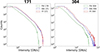 |
Fig. 1. Comparison of the logarithmic intensity distributions over test set 1 of the baseline-calibrated FSI observations (green), the ITI translations (red) generated from the FSI observations with the AIA observations as target, and the reference AIA observations (blue) for 171 Å (left) and 304 Å (right), respectively. |
We calculate the FID quality metric between the baseline calibrated FSI observation and the reference AIA observations, which we refer to as our baseline, and compare it with the FID calculated between the ITI and the reference AIA observations. Table 2 shows the perceptual quality assessment using the FID quality metric for the 171 Å and 304 Å channels, evaluated on test set 1 (Earth aligned). Lower FID values correspond to higher perceptual quality. With an FID of 3.5 for the 171 Å channel, ITI significantly outperforms the baseline calibration method, which has an FID of 9.9. Similar results are observed for the 304 Å channel, as shown in Table 2.
In Fig. 2 we evaluate the light curves by calculating the mean of each observed image and plotting it as a function of time. To ensure a statistically significant dataset for this comparison, the evaluation is performed on the entire FSI dataset, including the training data and test set 4 (light curve) until the end of January 2025. The FSI observations are baseline calibrated, where we shift the light curve to the mean and standard deviation of the AIA light curve according to Eq. (1). The mean and standard deviations are estimated over the entire training set for both FSI (2022–2023) and AIA (2011–2024). The first panel in Fig. 2a shows the time-shifted light curve in the 171 Å channel, and the second panel the 304 Å channel. The shaded-blue area along the AIA light curve corresponds to a ±1σ error range. The shaded-gray area represents the longitudinal position of Solar Orbiter outside of the FOV of SDO ranging from 113° to 248°. This is illustrated in panel b, where we indicate the related spacecraft constellations. We adjust the ITI and the baseline calibrated FSI observations according to the longitudinal difference of Solar Orbiter and with respect to SDO to allow for a more consistent comparison as described in Sect. 3.3. For large separation angles, as shown in the third panel in Fig. 2a, the results are more difficult to interpret, since during this time Solar Orbiter observed on the solar far side. The dashed red line in Fig. 2a indicates zero difference between the two spacecraft in longitude. The image calibration demonstrates robust performance across the entire period shown, with closer resemblance to the AIA ground truth than the baseline. Additionally, we evaluate the mean absolute error (MAE) of the baseline and ITI to the reference AIA light curve. Our ITI method achieves a value of 0.6 for the 171 Å, outperforming the baseline calibration with an MAE value of 14.4. Table 2 lists the MAE and FID values for both wavelengths.
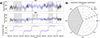 |
Fig. 2. Comparison between the light curves from January 2022 to January 2025 derived from the baseline-calibrated FSI data (green), the ITI translated data (red), and the reference AIA data (blue), including training data. The shaded-blue area corresponds to ±1σ error range from AIA. In a) the first panel corresponds to the 171 Å and the second to the 304 Å channel. The light curves were co-aligned in longitude using the separation angle between the SDO and Solar Orbiter spacecraft shown in the third panel. In b) the coordinate system is shown, with the shaded-gray area corresponding to the shaded-gray area in a), indicating that Solar Orbiter was located on the solar far side and thus not observing the same regions of the Sun as SDO. |
4.2. Qualitative comparison
Our ITI method allows for simultaneous image enhancement to match the reference distribution as closely as possible, in addition to image calibration. This has already been demonstrated for EUV instruments in previous applications of ITI, for example, for SOHO and STEREO (Jarolim et al. 2025). In Fig. 3, we show an example observation from test set 1 from March 20, 2024, at 16:00 UT. The distance of Solar Orbiter to the Sun is ΔD = 0.43 AU, and the difference in longitude and latitude between the Solar Orbiter and SDO spacecraft is ΔLON = 0.76° and ΔLAT = 0.67°, respectively. Figure 3 visualizes the full Sun observations as well as smaller cutouts. The cutouts are selected at random, with the aim of capturing both an active region and a quiet region. The first column corresponds to the baseline-calibrated FSI observations, the second column to our ITI translations, and the third column to the reference AIA observations. The first row shows the 171 Å channel, and the second row the 304 Å channel. The full Sun observations show that our ITI translations closely resemble the reference AIA observations on the global scale. The zoomed-in region indicates that enhanced features are visually similar to the structures observed by AIA on smaller scales. Where the baseline-calibrated FSI observation looks smoother with less contrast, the ITI translated observation appears sharper, and the intensities match the reference AIA observation closer. Similarly, in the 304 Å channel, the loop-like structure as well as the quiet Sun regions are represented sharper in ITI compared to the baseline calibrated FSI cutouts. Note that, even when Solar Orbiter is aligned with the Sun–Earth line, a persistent latitudinal offset between the two spacecraft introduces enhanced errors in pixel-based metrics and intensity ratio images.
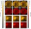 |
Fig. 3. Comparison of the baseline calibration, ITI, and the reference AIA observation from March 20, 2024, at 16:00 UT. The left column shows the baseline-calibrated FSI observations in 171 Å and 304 Å. The second column corresponds to our ITI translated observations, and the third row shows the reference AIA observations. The smaller cutouts shown in the lower rows correspond to the green and red squares in the full Sun observations. |
4.3. Distance comparison
Due to the varying orbit of Solar Orbiter, the spatial resolution of the observation also changes. For consistency, we resized and scaled all observations to 1.1 solar radii and a resolution of 1024 × 1024 pixels. To see how the distance influences the ITI translations, we tested the ITI tool on test set 2 (variable distance) covering observations from 0.31 AU to 0.89 AU. The results are illustrated in Fig. 4. We show six observations, each for a particular distance from Solar Orbiter to the Sun. The observations are cutouts with a size of 250″ × 250″. Each quad plot visualizes the baseline calibrated FSI observation in the left column for 174 Å and 304 Å channel and the right panel the corresponding ITI translations. We show observations at 0.31 AU, 0.39 AU, 0.50 AU, 0.70 AU, 0.80 AU, and 0.89 AU (from top left to bottom right).
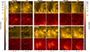 |
Fig. 4. Comparison of the baseline calibrated FSI observations with our ITI calibrations for six different distances of Solar Orbiter to the Sun. Each quad plot corresponds to a certain distance, where the left column corresponds to the EUI/FSI observation in 174 Å and 304 Å, and the right column to the corresponding ITI calibration. |
The examples in Fig. 4 illustrate how the spatial resolution decreases due to the radial distance of the Solar Orbiter spacecraft from the Sun. In the first row (0.31–0.50 AU), the difference between FSI and ITI is dominated by the intensity calibration aspect to AIA, which shows a similar quality in terms of sharpness of structures, but with the intensities adapted to AIA. The second row (0.70–0.89 AU) shows that the original FSI observations have a lower spatial resolution. The ITI translated observations show an increase in contrast that matches the AIA observations. However, as the distance between Solar Orbiter and the Sun increases, ITI can produce artifacts on small scales.
4.4. Multi-viewpoint application
With the highly elliptical orbit of Solar Orbiter, we can use ITI to provide joint data products with SDO/AIA and study the Sun from two different vantage points. We therefore used the third test set where Solar Orbiter was not Earth-aligned but part of its FOV overlap with the FOV of SDO from the Earth perspective. The test set spans from 21 October 2023 to 24 October 2023 (test set 3). The spacecraft position of Solar Orbiter (orange) and SDO (blue) is shown in Fig. 5. The separation angle of the two spacecraft in longitude across the test set ranges from 40° to 33°, where Solar Orbiter is west from SDO in longitude.
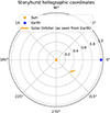 |
Fig. 5. Solar Orbiter spacecraft position for the multi-viewpoint test set. |
Figure 6 shows an example result of the test set from the 21 October 2023 at 00:00 UT. As in Fig. 3, we show the full Sun observations with smaller cutouts of an active region. The first column corresponds to the baseline calibrated FSI observations, the second column to the ITI translations, and the third column to the AIA observations. The first and second row show the observations in 171 Å and 304 Å, respectively. For the zoomed-in views, we cut out an active region located close to the disk center from Solar Orbiter’s perspective. The same active region is located on the eastern limb in the SDO/AIA perspective. A visual comparison on the global scale indicates that ITI shows a closer resemblance in contrast and quality to AIA compared to the baseline calibrated FSI, although they do not share the same FOV. Additionally, the quality of the zoomed-in regions is also higher, showing sharper contours for both 171 Å and 304 Å in ITI. The contrast difference between FSI, ITI, and AIA in both channels can be explained by a different line-of-sight integration, since the location of the active region for Solar Orbiter is at the disk center and closer to the limb for AIA. We point out that these inter-calibrated data products cannot be quantified because of the large separation angle of the two spacecraft.
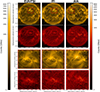 |
Fig. 6. Multi-viewpoint comparison between Solar Orbiter/EUI/FSI and SDO/AIA. The left column shows the baseline-calibrated FSI observations, the middle column the ITI translated, and the right column the AIA observations. The top row shows the 171 Å, and the bottom row the 304 Å channel. The smaller cutouts correspond to the red rectangles in the full Sun observations. |
5. Discussion and conclusion
We applied the ITI framework from Jarolim et al. (2025) to calibrate the FSI instrument on board Solar Orbiter with the AIA instrument on board SDO. The unpaired image translation approach allows for calibrating both instruments, which would not be achievable with paired image translation due to the sparse overlap of observations (Isola et al. 2017).
We compared our results against a standard baseline calibration, as described in Sect. 3.1. Comparing the light curves in Fig. 2, we see that ITI provides an improved calibration of the intensities and therefore outperforms the baseline calibration. This is also quantified in Table 2, where the MAE of ITI shows better image calibrations compared to the baseline. The comparison of the image distributions in Fig. 1 and the FID quality metric in Table 2 also confirms this for perceptual quality for both channels, where lower FID values correspond to higher perceptual quality. Comparing the calibrations of ITI for different distances of Solar Orbiter to the Sun in Fig. 4, we see that for close-in observations (0.3–0.5 AU) the intensity adjustment dominates, while the spatial resolution of the original FSI observation is high. In contrast, the spatial resolution of FSI decreases with distance, resulting in more blurred solar features. ITI is capable of adjusting the intensities but also enhances the observations, showing more details on smaller scales. However, this can also lead to small-scale artifacts in the ITI calibrations for both the 171 Å and 304 Å filters. Consequently, ITI provides homogeneous data series and can be used for both global and small-scale studies at distances of Solar Orbiter up to 0.5 AU from the Sun, due to the high spatial resolution of the FSI instrument. For distances greater than 0.5 AU, ITI can be used for studies on global scales. These distances should not be used for the study of small-scale features, as artifacts can appear at smaller scales. In addition, off-pointing SOOP observations cannot be used for ITI image calibration, as these observations show intensity variations in different regions on the solar disk that ITI cannot account for.
Figure 2 illustrates the importance of image calibration, as the Sun shows substantial variability over solar rotation and solar cycle time scales. The limitation here is that we cannot quantify these changes for ITI over a longer period, primarily due to the different orbital paths of Solar Orbiter and SDO. Multi-viewpoint observations are therefore essential for accurate quantification. Nevertheless, based on light assumptions, we show that ITI performs well on average for image calibration from different viewpoints as well as on the solar far side. As a result, ITI not only provides reliable calibrations across instruments but also enables pre- and post-estimations of solar EUV irradiance, with intensities adapted to AIA, as the Sun rotates in and out of Earth’s FOV (Woods et al. 1998; Lilensten et al. 2008).
In conclusion, ITI can effectively overcome limitations of standard image calibration methods, accounting for instrumental effects, filter characteristics, and quality differences by leveraging the fully data-driven approach of high-quality datasets (Hamada et al. 2020). The improved ITI calibrated observations enable more consistent solar cycle studies such as solar variability investigations where multi-instrument data need to be combined into a homogeneous data series (Ermolli et al. 2013). With the out-of-ecliptic transition of Solar Orbiter in 2025, ITI can be used to obtain calibrated data products that will allow studies of the Sun from multiple vantage points and outside the ecliptic plane (Saqri et al. 2022; Purkhart et al. 2024). Additionally, the results demonstrate that the calibrated ITI data products can be used for active regions and coronal hole evolution and detection (e.g., Jarolim et al. 2021; Delouille et al. 2018).
The next step involves making the ITI calibrated dataset available to the scientific community. The code used for the translations is already publicly accessible. Additionally, we aim to constantly update and integrate new data into the framework from future space missions, i.e., from the Joint EUV coronal Diagnostic Investigation (JEDI) imager on board the upcoming Vigil mission (Palomba & Luntama 2022), in order to provide a large database of homogenized data products.
Data availability
The code is publicly available in the following repository: https://github.com/spaceml-org/InstrumentToInstrument. In addition, we provide framework documentation with example Jupyter notebooks on our ReadTheDocs website: https://iti-documentation.readthedocs.io. All ITI models are publicly available at https://huggingface.co/SpaceML/ITI.
Acknowledgments
This research has received financial support from NASA award 22-MDRAIT22-0018 (No. 80NSSC23K1045) and managed by Trillium Technologies, Inc. The research was in part sponsored by the DynaSun project and has thus received funding under the Horizon Europe programme of the European Union under grant agreement (no. 101131534). Views and opinions expressed are however those of the author(s) only and do not necessarily reflect those of the European Union and therefore the European Union cannot be held responsible for them. CS was supported by the University of Graz EST (European Solar Telescope) program and the Guest Investigator Program of the Royal Observatory of Belgium (ROB). RJ was supported by the NASA Jack-Eddy Fellowship. LD was supported by the PRODEX Programme of the European Space Agency (ESA) under contract number 4000136424. We thankfully acknowledge David Berghmans for providing the Solar Orbiter data and the valuable comments to the paper. Solar Orbiter is a space mission of international collaboration between ESA and NASA, operated by ESA. The EUI instrument was built by CSL, IAS, MPS, MSSL/UCL, PMOD/WRC, ROB, LCF/IO with funding from the Belgian Federal Science Policy Office (BELSPO/PRODEX PEA 4000112292 and 4000134088); the Centre National d’Etudes Spatiales (CNES); the UK Space Agency (UKSA); the Bundesministerium für Wirtschaft und Energie (BMWi) through the Deutsches Zentrum für Luft- und Raumfahrt (DLR); and the Swiss Space Office (SSO). This research has made use of AstroPy (Astropy Collaboration 2022), SunPy (The SunPy Community et al. 2020) and PyTorch (Paszke et al. 2017).
References
- Aschwanden, M. J., Wülser, J.-P., Nitta, N. V., & Lemen, J. R. 2008, ApJ, 679, 827 [NASA ADS] [CrossRef] [Google Scholar]
- Astropy Collaboration (Price-Whelan, A. M., et al.) 2022, ApJ, 935, 167 [NASA ADS] [CrossRef] [Google Scholar]
- Barnes, W. T. M. Cheung, M. C., Bobra, M. G., et al. 2020, J. Open Source Softw., 5, 2801 [NASA ADS] [CrossRef] [Google Scholar]
- Berghmans, D., Auchère, F., Long, D. M., et al. 2021, A&A, 656, L4 [NASA ADS] [CrossRef] [EDP Sciences] [Google Scholar]
- Caplan, R. M., Downs, C., & Linker, J. A. 2016, ApJ, 823, 53 [CrossRef] [Google Scholar]
- Chitta, L. P., Zhukov, A. N., Berghmans, D., et al. 2023, Science, 381, 867 [NASA ADS] [CrossRef] [Google Scholar]
- Collier, H., Hayes, L., Purkhart, S., et al. 2024, A&A, 692, A176 [NASA ADS] [CrossRef] [EDP Sciences] [Google Scholar]
- Delouille, V., Hofmeister, S. J., Reiss, M. A., et al. 2018, Machine Learning Techniques for Space Weather (Elsevier), 365 [Google Scholar]
- Díaz Baso, C. J., & Asensio Ramos, A. 2018, A&A, 614, A5 [NASA ADS] [CrossRef] [EDP Sciences] [Google Scholar]
- Díaz Baso, C. J., de la Cruz Rodríguez, J., & Danilovic, S. 2019, A&A, 629, A99 [NASA ADS] [CrossRef] [EDP Sciences] [Google Scholar]
- Domingo, V., Fleck, B., & Poland, A. I. 1995, Sol. Phys., 162, 1 [Google Scholar]
- Dos Santos, L. F. G., Bose, S., Salvatelli, V., et al. 2021, A&A, 648, A53 [NASA ADS] [CrossRef] [EDP Sciences] [Google Scholar]
- Driesman, A., Hynes, S., & Cancro, G. 2008, Space Sci. Rev., 136, 17 [NASA ADS] [CrossRef] [Google Scholar]
- Ermolli, I., Matthes, K., Dudok de Wit, T., et al. 2013, Atmos. Chem. Phys., 13, 3945 [NASA ADS] [Google Scholar]
- Goodfellow, I., Pouget-Abadie, J., Mirza, M., et al. 2020, Commun. ACM, 63, 139 [CrossRef] [Google Scholar]
- Hamada, A., Asikainen, T., & Mursula, K. 2020, Sol. Phys., 295, 2 [NASA ADS] [CrossRef] [Google Scholar]
- Heusel, M., Ramsauer, H., Unterthiner, T., Nessler, B., & Hochreiter, S. 2017, in Proceedings of the 31st International Conference on Neural Information Processing Systems, (Red Hook, NY, USA: Curran Associates Inc.), NIPS’17, 6629 [Google Scholar]
- Isola, P., Zhu, J. Y., Zhou, T., & Efros, A. A. 2017, 2017 IEEE Conference on Computer Vision and Pattern Recognition (CVPR), 5967 [Google Scholar]
- Jarolim, R., Veronig, A. M., Hofmeister, S., et al. 2021, A&A, 652, A13 [NASA ADS] [CrossRef] [EDP Sciences] [Google Scholar]
- Jarolim, R., Tremblay, B., Muñoz-Jaramillo, A., et al. 2024, ApJ, 961, L31 [NASA ADS] [Google Scholar]
- Jarolim, R., Veronig, A., Pötzi, W., & Podladchikova, T. 2025, Nat. Commun., 16, 3157 [Google Scholar]
- Kim, T., Park, E., Lee, H., et al. 2019, Nat. Astron., 3, 397 [Google Scholar]
- Kraaikamp, E., Gissot, S., Stegen, K., et al. 2023, SolO/EUI Data Release 6.0 2023-01, https://doi.org/10.24414/z818-4163 (Royal Observatory of Belgium (ROB)) [Google Scholar]
- Lemen, J., Title, A., Akin, D., et al. 2012, Sol. Phys., 275, 17 [NASA ADS] [CrossRef] [Google Scholar]
- Lilensten, J., Dudok de Wit, T., Kretzschmar, M., et al. 2008, Ann. Geophys., 26, 269 [Google Scholar]
- Müller, D., St. Cyr, O. C., Zouganelis, I., et al. 2020, A&A, 642, A1 [Google Scholar]
- Nisticó, G., Polito, V., Nakariakov, V. M., & Del Zanna, G. 2017, A&A, 600, A37 [NASA ADS] [CrossRef] [EDP Sciences] [Google Scholar]
- O’Kane, J., Green, L. M., Davies, E. E., et al. 2021, A&A, 656, L6 [NASA ADS] [CrossRef] [EDP Sciences] [Google Scholar]
- Palomba, M., & Luntama, J. P. 2022, in 44th COSPAR Scientific Assembly. Held 16–24 July, 44, 3544 [Google Scholar]
- Paszke, A., Gross, S., Chintala, S., et al. 2017, in NIPS-W [Google Scholar]
- Pesnell, W., Thompson, B., & Chamberlin, P. 2012, Sol. Phys., 275, 3 [Google Scholar]
- Podladchikova, T., Jain, S., Veronig, A. M., et al. 2024, A&A, 691, A344 [NASA ADS] [CrossRef] [EDP Sciences] [Google Scholar]
- Pötzi, W., Veronig, A., Jarolim, R., et al. 2021, Sol. Phys., 296, 164 [CrossRef] [Google Scholar]
- Purkhart, S., Veronig, A. M., Kliem, B., et al. 2024, A&A, 689, A259 [NASA ADS] [CrossRef] [EDP Sciences] [Google Scholar]
- Reiss, M. A., Muglach, K., Möstl, C., et al. 2021, ApJ, 913, 28 [Google Scholar]
- Rochus, P., Auchère, F., Berghmans, D., et al. 2020, A&A, 642, A8 [NASA ADS] [CrossRef] [EDP Sciences] [Google Scholar]
- Ronneberger, O., Fischer, P., & Brox, T. 2015, in Medical Image Computing and Computer-Assisted Intervention – MICCAI 2015, eds. N. Navab, J. Hornegger, W. M. Wells, & A. F. Frangi (Cham: Springer International Publishing), 234 [Google Scholar]
- Saqri, J., Veronig, A. M., Warmuth, A., et al. 2022, A&A, 659, A52 [NASA ADS] [CrossRef] [EDP Sciences] [Google Scholar]
- Saqri, J., Veronig, A. M., Battaglia, A. F., et al. 2024, A&A, 683, A41 [NASA ADS] [CrossRef] [EDP Sciences] [Google Scholar]
- Schirninger, C., Jarolim, R., Veronig, A. M., & Kuckein, C. 2024, A&A, 693, A6 [Google Scholar]
- Schwanitz, C., Harra, L., Mandrini, C. H., et al. 2023, A&A, 674, A219 [NASA ADS] [CrossRef] [EDP Sciences] [Google Scholar]
- The SunPy Community, Barnes, W. T., Bobra, M. G., et al. 2020, ApJ, 890, 68 [NASA ADS] [CrossRef] [Google Scholar]
- Tsuneta, S., Ichimoto, K., Katsukawa, Y., et al. 2008, Sol. Phys., 249, 167 [Google Scholar]
- Usoskin, I., & Mursula, K. 2003, Sol. Phys., 218, 319 [Google Scholar]
- Wang, T. C., Liu, M. Y., Zhu, J. Y., et al. 2018, in 2018 IEEE/CVF Conference on Computer Vision and Pattern Recognition, 8798 [Google Scholar]
- Woods, T. N., Rottman, G. J., Bailey, S. M., Solomon, S. C., & Worden, J. R. 1998, in Solar Electromagnetic Radiation Study for Solar Cycle 22: Proceedings of the SOLERS22 Workshop held at the National Solar Observatory, Sacramento Peak, Sunspot, New Mexico, USA, June 17–21, 1996 (Springer), 133 [Google Scholar]
- Woods, T. N., Eparvier, F., Hock, R., et al. 2012, The Solar Dynamics Observatory (Springer), 115 [Google Scholar]
- Youn, J., Lee, H., Jeong, H.-J., et al. 2025, A&A, 695, A125 [NASA ADS] [CrossRef] [EDP Sciences] [Google Scholar]
- Zhu, J. Y., Park, T., Isola, P., & Efros, A. A. 2017, in 2017 IEEE International Conference on Computer Vision (ICCV), 2242 [Google Scholar]
- Zouganelis, I., De Groof, A., Walsh, A. P., et al. 2020, A&A, 642, A3 [NASA ADS] [CrossRef] [EDP Sciences] [Google Scholar]
Appendix A: Degradation correction
We perform a degradation correction analysis for the EUI/FSI instrument as described in Sect. 2.1. The analysis is performed over the training set from January 2022 to May 2023 and is shown in Fig. A.1. We extract the quiet Sun from full-Sun observations using a thresholding method. The threshold is set according to the median intensity plus the standard deviation of each observation. All regions with values below this threshold are considered to represent the quiet Sun. In Fig. A.1 we plot the quiet Sun mean intensities in blue, the linear fit in black and the corrected light curve in red for both the the 174 Å and the 304 Å channel. We have performed the degradation analysis up to the latest available data in 2025. However, the degradation fit parameters do not change significantly. Consequently, the degradation correction until 2023 is sufficient to model the degradation up to 2025.
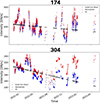 |
Fig. A.1. Degradation correction for the EUI/FSI 174 Å (first panel) and 304 Å channel (second panel) over the training set from January 2022 to May 2023. The blue line corresponds to the quiet Sun mean intensities, the black line to the linear fit, and the red line to the corrected light curve. |
Appendix B: Histogram comparison
To show that ITI can provide robust image calibration we calculate the histograms for 171 Å and 304 Å over test set 1 (Earth aligned) for the on-disk and off-limb pixels. In Fig B.1 the first row shows the on-disk histograms on a logarithmic scale with AIA in blue, ITI in red and the baseline FSI in green, same as in Fig.1. The second row shows the off-limb histogram. For both, ITI (red) matches the AIA distribution (blue) closer than the baseline calibrated FSI observations (green).
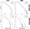 |
Fig. B.1. Comparison of the logarithmic intensities for AIA (blue), ITI (red), and the baseline calibrated FSI (green) over test set 1 (Earth-aligned). The first row shows the on-disk histogram, and the second row the off-limb histogram for the 171 Å and the 304 Å channel. |
All Tables
Number of observations of the dataset split into training, validation, and three different test sets.
All Figures
|
Fig. 1. Comparison of the logarithmic intensity distributions over test set 1 of the baseline-calibrated FSI observations (green), the ITI translations (red) generated from the FSI observations with the AIA observations as target, and the reference AIA observations (blue) for 171 Å (left) and 304 Å (right), respectively. |
| In the text | |
|
Fig. 2. Comparison between the light curves from January 2022 to January 2025 derived from the baseline-calibrated FSI data (green), the ITI translated data (red), and the reference AIA data (blue), including training data. The shaded-blue area corresponds to ±1σ error range from AIA. In a) the first panel corresponds to the 171 Å and the second to the 304 Å channel. The light curves were co-aligned in longitude using the separation angle between the SDO and Solar Orbiter spacecraft shown in the third panel. In b) the coordinate system is shown, with the shaded-gray area corresponding to the shaded-gray area in a), indicating that Solar Orbiter was located on the solar far side and thus not observing the same regions of the Sun as SDO. |
| In the text | |
|
Fig. 3. Comparison of the baseline calibration, ITI, and the reference AIA observation from March 20, 2024, at 16:00 UT. The left column shows the baseline-calibrated FSI observations in 171 Å and 304 Å. The second column corresponds to our ITI translated observations, and the third row shows the reference AIA observations. The smaller cutouts shown in the lower rows correspond to the green and red squares in the full Sun observations. |
| In the text | |
|
Fig. 4. Comparison of the baseline calibrated FSI observations with our ITI calibrations for six different distances of Solar Orbiter to the Sun. Each quad plot corresponds to a certain distance, where the left column corresponds to the EUI/FSI observation in 174 Å and 304 Å, and the right column to the corresponding ITI calibration. |
| In the text | |
|
Fig. 5. Solar Orbiter spacecraft position for the multi-viewpoint test set. |
| In the text | |
|
Fig. 6. Multi-viewpoint comparison between Solar Orbiter/EUI/FSI and SDO/AIA. The left column shows the baseline-calibrated FSI observations, the middle column the ITI translated, and the right column the AIA observations. The top row shows the 171 Å, and the bottom row the 304 Å channel. The smaller cutouts correspond to the red rectangles in the full Sun observations. |
| In the text | |
|
Fig. A.1. Degradation correction for the EUI/FSI 174 Å (first panel) and 304 Å channel (second panel) over the training set from January 2022 to May 2023. The blue line corresponds to the quiet Sun mean intensities, the black line to the linear fit, and the red line to the corrected light curve. |
| In the text | |
|
Fig. B.1. Comparison of the logarithmic intensities for AIA (blue), ITI (red), and the baseline calibrated FSI (green) over test set 1 (Earth-aligned). The first row shows the on-disk histogram, and the second row the off-limb histogram for the 171 Å and the 304 Å channel. |
| In the text | |
Current usage metrics show cumulative count of Article Views (full-text article views including HTML views, PDF and ePub downloads, according to the available data) and Abstracts Views on Vision4Press platform.
Data correspond to usage on the plateform after 2015. The current usage metrics is available 48-96 hours after online publication and is updated daily on week days.
Initial download of the metrics may take a while.