| Issue |
A&A
Volume 703, November 2025
|
|
|---|---|---|
| Article Number | A24 | |
| Number of page(s) | 8 | |
| Section | Planets, planetary systems, and small bodies | |
| DOI | https://doi.org/10.1051/0004-6361/202556404 | |
| Published online | 30 October 2025 | |
Magnetohydrodynamic simulation assessment of a potential near-ultraviolet early ingress in WASP-189b
1
Globe Institute–Center for Star and Planet Formation, University of Copenhagen,
Copenhagen,
Denmark
2
Department of Space Science and Engineering, National Central University,
Taoyuan,
Taiwan
3
Center for Astronautical Physics and Engineering, National Central University,
Taoyuan,
Taiwan
4
Department of Physics-Lund Observatory, Lund University,
Lund,
Sweden
5
Institute of Astronomy, National Central University,
Taoyuan,
Taiwan
6
Steward Observatory, The University of Arizona,
Tucson,
AZ,
USA
7
Shanghai Astronomical Observatory, Chinese Academy of Sciences,
Shanghai,
China
8
Laboratory for Atmospheric and Space Physics, University of Colorado Boulder,
Boulder,
CO,
USA
9
Space Research Institute, Austrian Academy of Sciences,
Graz,
Austria
★ Corresponding authors: This email address is being protected from spambots. You need JavaScript enabled to view it.
; This email address is being protected from spambots. You need JavaScript enabled to view it.
Received:
14
July
2025
Accepted:
17
September
2025
Abstract
Context. Ultra-hot Jupiters (UHJs) in close orbits around early-type stars provide natural laboratories for studying atmospheric escape and star-planet interactions under extreme irradiation and wind conditions. The near-ultraviolet (NUV) regime is particularly sensitive to extended upper atmospheric and magnetospheric structures.
Aims. We investigate whether star-planet interactions in the WASP-189 system could plausibly account for the early ingress feature suggested by NUV transit fitting models.
Methods. We analysed three NUV transits of WASP-I89b observed as part of the Colorado Ultraviolet Transit Experiment (CUTE), which employs a 6U CubeSat dedicated to exoplanet spectroscopy. To explore whether the observed transit asymmetry could plausibly arise from a magnetospheric bow shock (MBS), we performed magnetohydrodynamic (MHD) simulations using representative stellar wind velocities and planetary atmospheric densities.
Results. During Visit 3, we identified a ~31.5-minute phase offset that is consistent with an early ingress. Our MHD simulations indicate that, with a wind speed of 572.97 km s−1 and a sufficient upper atmospheric density (~4.59 × 10⁻¹¹ kg m−3), a higher-density zone due to compression can form ahead of the planet within five planetary radii in regions where the fast-mode Mach number falls below ~0.56, even without a MBS. Shock cooling and crossing time estimates from the simulations further suggest that such a pileup could, in principle, produce detectable NUV absorption.
Conclusions. Our results indicate that while MBS formation is feasible for WASP-189b, low stellar-wind speeds favour NUV-detectable magnetic pileups over classical bow shocks. Immediately after the shock formation, the post-shock plasma is too hot for strong NUV absorption, but a high-to-low wind-speed transition shortens the cooling time while preserving the compressed plasma, increasing its opacity. Pressure-balance estimates show that magnetic pressure dominates across wind regimes in the low-density case, and at low wind speeds in the high-density case, favouring pileup and reconnection near the magnetopause and enhancing the potential detectability of early-ingress signatures.
Key words: planets and satellites: atmospheres / planets and satellites: gaseous planets / planets and satellites: magnetic fields / planet-star interactions / ultraviolet: planetary systems
© The Authors 2025
 Open Access article, published by EDP Sciences, under the terms of the Creative Commons Attribution License (https://creativecommons.org/licenses/by/4.0), which permits unrestricted use, distribution, and reproduction in any medium, provided the original work is properly cited.
This article is published in open access under the Subscribe to Open model. This email address is being protected from spambots. You need JavaScript enabled to view it. to support open access publication.
1 Introduction
Ultra-hot Jupiters (UHJs), orbiting close to luminous stars, are exposed to extreme irradiation, which drives atmospheric expansion, rapid mass loss, and metal-enriched exo-spheres (Parmentier et al. 2018; Helling et al. 2019; Arcangeli et al. 2018; Lothringer et al. 2018; Hoeijmakers et al. 2019). These systems serve as natural laboratories for studying atmospheric dynamics and star-planet interactions, particularly via near-ultraviolet (NUV) transmission spectroscopy (Lai et al. 2010; Llama et al. 2011; Vidotto et al. 2011; Alexander et al. 2015; Stangret et al. 2021). NUV transit anomalies, such as the early ingress (EI) reported for WASP-12b, have been interpreted as possible signatures of planetary magnetospheric bow shocks (MBSs; Vidotto et al. 2010, 2011; Llama et al. 2011; Haswell et al. 2012; Wong et al. 2022), with simulations highlighting the key role of magnetic topology in shaping stellar wind-planet interactions (Debrecht et al. 2018; Daley-Yates & Stevens 2019). However, the MBS scenario remains debated, as models indicate that shock cooling timescales may be too long to produce sufficient NUV opacity (Alexander et al. 2015).
WASP-189b, a UHJ orbiting the A-type star HD 133112 every ~2.72 days, exhibits extreme dayside temperatures (>3400 K), a highly inclined orbit, and pronounced stellar gravity darkening (Lendl et al. 2020; Deline et al. 2022; Yan et al. 2020). Observations reveal an extended, metal-rich upper atmosphere and signatures suggestive of complex magnetospheric interactions (Prinoth et al. 2022, 2023; Sreejith et al. 2023). Motivated by the fitted NUV EI in this system, we investigated whether such features can plausibly arise from star-planet interaction processes, such as MBS formation, or due to zones of higher density, and discuss their implications for atmospheric escape and magnetospheric dynamics in UHJs.
Input parameters and best-fit results from the MCMC analysis.
2 Observations and data analysis
2.1 CUTE NUV transit observations and fittings
WASP-189b was observed in the NUV (2479−3306 Å, R ~ 750 W) by the Colorado Ultraviolet Transit Experiment (CUTE) 6U CubeSat, which enables consecutive transit coverage thanks to its 96-minute orbit (Sreejith et al. 2023; France et al. 2023). We analysed the same three-transit dataset as Sreejith et al. (2022, 2023), processed with their pipeline, excluding exposures with jitter > 6″ or charge-coupled device (CCD) temperatures >−5 °C. VI includes 13 orbits; V2 and V3 include 16 each, over phases −0.2 to +0.2.
White-light curves were constructed by integrating all wave-lengths and fluxes reported in detector counts. Systematics were corrected with polynomial fits and robust transit parameters obtained via Markov chain Monte Carlo (MCMC) analysis. Transmission spectra were extracted using the ‘divide-white’ method (Kreidberg et al. 2014). Due to limited S/N, spectral anomalies could not be attributed to specific species.
Transit fitting with batman and emcee (Kreidberg 2015; Foreman-Mackey et al. 2013), using CHEOPS parameters (Lendl et al. 2020) and PHOENIX limb-darkening, produced generally good fits (Table 1). For V3, a ~31.5-minute ingress offset was found (Fig. 1), corresponding to a possible absorbing extension to ~3.65 Rp based on standard geometric calculations (Anderson et al. 2018). The RMS residual (~10−3) supports the model quality, but the physical origin of this offset remains unknown. In this work, we assessed whether a MBS could produce the EI signature in WASP-189b, treating the measured offset as an upper bound. Our Bayesian analysis (Appendix B) yields moderate evidence of an EI feature in Visit 3 (V3). A uniform phase correction was applied across all transits for consistency, and limited phase coverage renders this feature tentative; related Mg II spectral variations are shown in Fig. A.1.
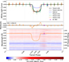 |
Fig. 1 CUTE NUV transit and spectral analysis for WASP-189b. Top: White-light curves for three visits (V1, V2, and V3; coloured points) and all data combined, with best-fit transit models (dashed lines) and uncertainties (grey shading). The magenta star marks Event 662 in V3. Middle: residuals relative to best-fit models for each visit and all data, highlighting deviations in V3 (orange). Bottom: Spectral map for V3: flux as a function of wavelength and phase, normalised to the continuum/ The colour scale shows fractional deviations. Anomalous features after egress (Event 662) indicate transient variability. |
2.2 Mass-loss and stellar wind constraints
The stellar wind environment at WASP-189b is estimated using escape velocity ( ), which yields υesc≈573 km s−1 for WASP-189. Based on line-driven wind theory (Castor et al. 1975), the terminal wind speed is typically υsw = [1, 3] υesc, corresponding to 573–1719 km s−1. In the intermediate- and high-speed regimes of this range, υsw exceeds the solar wind upper limit (850 km s−1; Alissandrakis & Gary 2021; Pevtsov et al. 2021). Theoretical models further suggest that fast-rotating A-type stars, like WASP-189 (Prot≈1.24 days; Lendl et al. 2020; Deline et al. 2022), can drive even higher wind speeds, consistent with the adopted simulation values (Johnstone et al. 2015).
A-type stars’ coronal activity, relevant for wind properties, is not always well constrained. WASP-189’s Teff=7996 K is near the threshold for weak coronal emission (Günther et al. 2022), analogous to Altair (A7 V) with Tcor ~ 106 K (Güdel 2004). This coronal temperature is used in our subsequent density calculations. The number density at the planetary orbital distance was then estimated following Vidotto et al. (2010):
![Mathematical equation: ${{{n_{{\rm{obs}}}}} \over {{n_0}}} = \exp \left[ {{{G{M_{\rm{s}}}/{R_{\rm{s}}}} \over {{k_{\rm{B}}}{T_{{\rm{cor}}}}/m}}\left( {{{{R_{\rm{s}}}} \over {{R_{{\rm{obs}}}}}} - 1} \right) + {{2{\pi ^2}R_{\rm{s}}^2/P_{\rm{s}}^2} \over {{k_{\rm{B}}}{T_{{\rm{cor}}}}/m}}\left( {{{R_{{\rm{orb}}}^2} \over {R_{\rm{s}}^2}} - 1} \right)} \right].$](/articles/aa/full_html/2025/11/aa56404-25/aa56404-25-eq8.png) (1)
(1)
Here, n0 is the coronal base number density, derived from mass continuity  (Lanz & Catala 1992) with Ṁ ~ 2 × 10⁻¹⁰ M⊙ yr−1. The base wind speed is taken as the isothermal sound speed,
  (Lamers & Cassinelli 1999), with Tb ~ 8000 K and µ ~ 0.6. Then,
  and n0 = ρ0/(µmp).
Applying these relations, we estimate the stellar wind density at the orbital distance of WASP-189b to be ρsw ≈ 5.32 × 10⁻¹³ kg m−3. The condition for bow-shock formation is set by the fast-mode magnetosonic Mach number, MF = υsw/Cf (Lai et al. 2024), where the fast magnetosonic speed is  . Here
  is the Alfvén speed, with µ0 denoting the vacuum permeability, and
  is the adiabatic sound speed for a monatomic, fully ionised gas, where γ = 5/3, Tcor is the coronal temperature, µ is the mean molecular weight, and mp is the proton mass.
To achieve MF > 1, a plasma density ≳10−11 kg m−3 is required. Since the ambient wind is less dense, local enhancement from the planetary upper atmosphere and magnetosheath compression is plausible. For UHJs, the wind-atmosphere interface is diffuse and variable, so ρ ~ ρatm is assumed for the stellar-wind downstream region here, estimated via ρ = µ mp p/(kB, Tp) (Rapp-Kindner et al. 2024) with Tp = 3435 K and p = 1 mPa, giving ρatm ~ 4.59 × 10⁻¹¹ kg m−3—above the shock-formation threshold and consistent with NUV variability under suitable wind conditions.
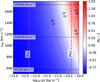 |
Fig. 2 Fast-mode magnetosonic Mach number under WASP-189b-like stellar wind conditions. The colour map shows MF − 1 as a function of log10(ρ) and υsw, for a stellar magnetic field of 79.05 G. White contours mark the MF = 1 boundary. Vertical magenta lines indicate estimated planetary upper atmosphere and stellar wind densities; horizontal dashed lines denote wind speeds of 1−3υesc. Regions where MF > 1 are conducive to bow shock formation. |
3 Magnetohydrodynamic simulations
To investigate the connection between WASP-189b’s early NUV ingress and the formation of a MBS, we mapped the fast-mode Mach number (MF) as a function of plasma density and stellar wind velocity using 2D ideal magnetohydrodynamic (MHD) simulations (Appendix E). The simulations adopt wind speeds of 1−3 υesc, plasma densities of either ρatm or ρsw, and stellar and planetary magnetic fields of 79.05 G and 60.22 G, respectively (Appendices C and D).
Figure 2 shows that MF exceeds unity – allowing bow shock formation – only when both stellar wind velocity and plasma density are sufficiently high, specifically for υsw ≳ 2υesc and ρ = ρatm. For typical stellar wind densities (ρsw), the flow remains sub-magnetosonic and no shock is produced, consistent with MHD theory and prior results (Alexander et al. 2015). Figure 3 further illustrates that clear, well-defined bow shocks emerge only under these high-υsw, high-ρ conditions; lower wind speeds generate only broad, diffuse density enhancements. The maximum spatial extent of these structures (up to ~5 Rp) is comparable to the ~3.7 Rp absorption region inferred from the EI, linking the MF parameter space (Fig. 2) with the simulated density morphologies (Fig. 3).
Overall, while our simulations confirm that MBS formation is dynamically feasible for WASP-189b, the detectability of such structures in the NUV is constrained by shock cooling physics. Detectable NUV absorption requires that the radiative cooling time (τcool) be shorter than the shock crossing time (τcross). As shown in Appendix G, this criterion is satisfied only for moderate stellar wind speeds (υsw = 572.97 km s−1) when the shock thickness lies within 2.45–2.94 Rp (Appendix F), enabling rapid cooling and sufficient NUV opacity.
At higher wind speeds, a bow shock can still form due to supersonic flow; however, the post-shock region remains too hot for efficient NUV absorption, rendering it effectively invisible at these wavelengths. If the stellar wind subsequently transitions from a high-speed to a low-speed regime, τcool decreases while the compressed plasma in the pileup region remains dense. Under these conditions, the cooled, optically thick sheath ahead of the magnetosphere can persist long enough to be observed in the NUV, potentially producing the EI signature (Table G.1). This scenario links the dynamic MBS formation seen in our simulations with the radiative conditions necessary for observational detection.
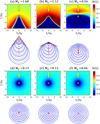 |
Fig. 3 2D MHD simulations of bow shock formation for WASP-189b under varying stellar wind conditions. Six combinations of stellar wind speed (υsw = 1−3υesc) and plasma density (ρatm or ρsw), with a stellar magnetic field of 79.05 G, are shown. Top: magnetic field strength (contours) and wind streamlines (yellow arrows); black circle marks the magnetopause stand-off distance (Rmp = 1.09–1.58 Rp). Bottom: fast-mode wavefronts and shock cones (brown), showing bow shock formation only for MF > 1. Panels a and b demonstrate that high υsw combined with high ρ is required for a distinct bow shock. |
4 Discussions and conclusions
CUTE NUV transit observations of WASP-I89b reveal a possible EI in V3 that was absent in V1 and V2. This suggests episodic, potentially wind-driven variability in the planet’s upper atmosphere. Similar anomalies in other hot Jupiters have been attributed to magnetospheric interactions or bow shocks (Vidotto et al. 2010; Llama et al. 2011; Sreejith et al. 2023), although our dataset does not confirm their persistence.
We assessed whether the observed signature could arise from MBS effects. Our MHD simulations show that classical MBS formation (MF > 1) requires both a high stellar wind velocity and sufficient plasma density. However, shock-cooling constraints indicate that only moderate winds (υsw ≈ υesc) enable rapid post-shock cooling and adequate NUV opacity. In this regime, a transient high-density pileup can form within ≲5 Rp ahead of the planet, consistent with the ~3.65 Rp absorption extent inferred from V3.
Moreover, comparison of the shock cooling time and shock crossing time indicates that NUV detectability is suppressed at the moment of MBS formation (Table G.1): the post-shock plasma remains too hot for efficient absorption, and by the time it cools sufficiently, the shock structure has already evolved from its initial state. If this evolution is followed by a transition from high to low stellar-wind speeds, EI visibility can increase substantially because the shorter τcool at lower υsw allows the residual compressed plasma to cool while maintaining a high density. The pressure budget at Rmp (Table D.1) supports this scenario: in the low-density case, magnetic pressure dominates over ram pressure across all wind speeds, and in the high-density case it dominates at low wind speeds. Such magnetic pileup ahead of the magnetosphere can facilitate dayside reconnection, channelling cooled plasma into the compressed sheath and increasing its NUV opacity – thereby favouring EI detection following a fast-to-slow wind transition.
In summary, while the true origin of the CUTE V3 offset remains uncertain, our study examines the possibility that NUV EI signatures in WASP-189b could arise from stellar-wind compression of the UHJ’s magnetosphere and associated plasma pileup. Our Bayesian analysis yields moderate evidence consistent with an EI feature in V3. This scenario highlights the value of coordinated, high-cadence UV and X-ray monitoring to better constrain stellar-wind conditions, assess planetary magnetic field strengths, and evaluate the predicted sensitivity of EI visibility to variations in wind properties.
Data availability
CUTE NUV transit data are available from the mission PI (K. France) on request. CHEOPS optical data are public via the ESA CHEOPS archive (https://www.ssdc.asi.it/cheops/) and as supplementary files in Lendl et al. (2020). Processed data and analysis scripts are available from the corresponding author upon request.
Acknowledgements
This work was supported by the Upper Air Dynamics Laboratory and CAPE at National Central University (NCU), with funding from NSTC grants 114-2917-I-564-044, 113-2111-M-008-007, 112-2811-M-008-072, 113-2811-M-008-001, 114-2111-M-008-008, and the Higher Education SPROUT grant from Taiwan’s Ministry of Education. H.J.H. acknowledges eSSENCE (eSSENCE@LU 9:3), the Swedish National Research Council (2023-05307), the Crafoord Foundation, and the Royal Physiographic Society of Lund. A.J. is supported by the Carlsberg Foundation (FIRSTATMO). We thank the CUTE team at the University of Colorado and the NCU Upper Air Dynamics Laboratory for data provision and downlink support. Y.D. thanks A. Johansen (U. Copenhagen) for hosting, G. Chen (PMO, CAS) for feedback, C.-H. Lin, J.-Y. Liu, Y.-C. Wen (NCU) for planetary and magnetospheric discussions, U.G. Jørgensen (NBI) for spectral advice, Y. Tian (Sejong U.) for UHJ discussions, and Y.-C. Chiu and R.-T. Chen for CUTE ground station support. An anonymous COSPAR 45 attendee is thanked for suggesting this investigation.
Appendix A Phase-dependent NUV spectral variability around Mg II
Spectral analysis around Mg II (2765.6–2834.6 Å) reveals time-dependent anomalies in V3 (e.g. emission at ingress, strong absorption post-egress) and V2, but not in V1. The rapid variability suggests temporal changes in the planet’s upper atmosphere or magnetospheric environment, though precise identification is limited by the S/N.
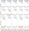 |
Fig. A.1 Phase-resolved spectral analysis of WASP-189 b around the Mg II region (2765.6–2834.6 Å). Each panel shows the flux variation (counts, not normalised) as a function of wavelength for different observational visits (V1, V2, and V3) and phase bins (Ph). The symbol # indicates the number of samples in each bin, while St and Ed denote the start and end phases, respectively. The grey markers represent the mean flux profile across multiple observations, with error bars indicating the standard deviation. Three specific events (557, 641, and 662) that deviate from the mean trend are highlighted in orange. The dashed red line denotes the median continuum level for each visit. These results provide insights into the temporal and phase-dependent variations in the observed spectral features, offering constraints on the atmospheric and astrophysical processes affecting WASP-189 b. |
Appendix B Early ingress and the Bayes factor
To test for the presence of an EI absorption feature in the NUV light curves, we constructed a phase-shifted replica of the fiducial transit model using the batman package (Kreidberg 2015). As illustrated in Fig. B.1, the observed light curves for each visit (grey for all visits, black for the highlighted one) are compared against two models: the nominal planet-only transit (blue solid line) and the planet+EI model (dashed orange line). The replica model adopts the same geometric parameters as the optical transit, and the only additional degree of freedom is a phase offset Δϕ, which shifts the centre of the replica earlier relative to the nominal transit (negative Δϕ corresponds to earlier ingress). The composite flux is then defined pointwise as
![Mathematical equation: ${F_{{\mathop{\rm model}\nolimits} }}\left( \phi \right) = \min \,\left[ {{F_{{\rm{base}}}}\left( \phi \right),\,{F_{{\rm{shift}}}}\left( {\phi + \Delta \phi } \right)} \right],$](/articles/aa/full_html/2025/11/aa56404-25/aa56404-25-eq15.png) (B.1)
(B.1)
where Fmodel(ϕ) is the combined flux at orbital phase ϕ, Fbase(ϕ) is the nominal planet-only transit, Fshift(ϕ + Δϕ) is the shifted replica, ϕ denotes the orbital phase relative to mid-transit (ϕ = 0), and Δϕ is the free phase-lead parameter.
Bayesian model comparison was carried out using the Bayes factor, defined as the ratio of the marginal likelihoods (Bayesian evidence) of two competing models (Jeffreys 1948; Kass & Raftery 1995; Heller & Hippke 2024). The evidence, 𝒵, was estimated with nested sampling, yielding
 (B.2)
(B.2)
where 𝒵EI and 𝒵base denote the evidence for the planet+EI and planet-only models, respectively. Positive values of 2 ln B favour the EI hypothesis, and the results can be interpreted according to the Jeffreys scale. In practice, log 𝒵EI was obtained from nested sampling (via UltraNest). For the baseline planet-only model, we used its maximum Gaussian log-likelihood as a proxy for log 𝒵base.
Applying this framework to the three NUV visits, and restricting the analysis to the transit phase interval −0.05 ≤ ϕ ≤ −0.01 in order to isolate the ingress region, we find negative Bayes factor values for the first two (2 ln B ≈ −7.87 and −4.46), indicating no preference for the EI model. By contrast, the third visit yields 2 ln B ≈ 3.78, corresponding to moderate statistical support for an EI feature within this pre-ingress window.
Appendix C Hot Jupiter surface magnetic field
We estimated the surface magnetic field strength Bsurf of WASP-189b using the scaling approach described by Dietrich et al. (2022), which is based on the Christensen dynamo scaling law (Christensen et al. 2009). This method relates a planet’s magnetic field to its internal heat flux under the assumption that the magnetic energy is set by the convective power available in the dynamo region. Their model assumes that the dynamo operates in a rapidly rotating, electrically conducting shell, that convection is driven by the internal heat flux, qint, and that the ohmic dissipation is small compared to the available convective power. The theory builds on magnetostrophic balance and energy-based scaling arguments (Christensen et al. 2009), which have been successfully applied to both Solar System and exoplanetary giant planets.
For WASP-189b, we estimated qint from its equilibrium temperature (Teq) using the empirical relation (Thorngren & Fortney 2018; Sarkis et al. 2021) as adopted by Dietrich et al. (2022):
![Mathematical equation: ${T_{{\mathop{\rm int}} }} = 0.39\,{T_{{\rm{eq}}}}\,\exp \left[ { - {{{{\left( {{{\log }_{10}}\left( {{\sigma _{{\rm{SB}}}}T_{{\rm{eq}}}^4} \right) - 6.14} \right)}^2}} \over {1.095}}} \right],$](/articles/aa/full_html/2025/11/aa56404-25/aa56404-25-eq17.png) (C.1)
(C.1)
 (C.2)
(C.2)
where Tint is the internal temperature, Teq is the planetary equilibrium temperature, and σSB is the Stefan–Boltzmann constant. We adopted Jupiter’s internal heat flux qint,J = 5.4 W m−2 and surface magnetic field BJ = 4.17 × 10⁻⁴ T as reference values (Dietrich et al. 2022).
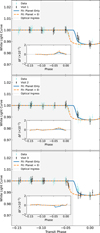 |
Fig. B.1 Per-visit comparison between the nominal transit model and the phase-shifted EI model. Each row corresponds to one WASP-189b transit (V1–V3). The main panels display the observed white light curves (cyan for all visits, black for the highlighted visit) together with the best-fitting models: the nominal planet-only transit (solid blue) and the planet+EI model (dashed orange). The insets show the corresponding residuals, ΔF, relative to each model. The EI model is constructed as the pointwise minimum of the base transit and a phase-shifted replica, providing a diagnostic test for the presence of an earlier ingress. |
The surface magnetic field was then obtained from the scaling law:
 (C.3)
(C.3)
where MJ and RJ are Jupiter’s mass and radius. This approach avoids assumptions on planetary age, instead inferring qint from Teq, which is particularly suitable for highly irradiated planets such as WASP-189b. Applying this method to WASP-189b yields an estimated surface magnetic field strength of Bsurf ≈ 60.22 G.
Appendix D Magnetopause and pressure budget
Direct measurements of WASP-189b’s magnetic field are unavailable currently; however, rapidly rotating A-type stars (such as WASP-189, Prot=1.24 days; Lendl et al. 2020; Deline et al. 2022) are expected to possess strong surface fields, often exceeding 7500 G (Mathys 2017). Assuming a dipole geometry, the stellar field at the planet’s orbit (r=0.05 AU) follows B(r)=B0(R0/r)3, giving ~79.05 G for our MHD models.
The dayside magnetopause stand-off distance of WASP-189b is computed using the magnetodisc–dipole formulation of Khodachenko et al. (2012), which is based on a paraboloid magnetospheric model and accounts for the extended magnetodiscs of hot Jupiters that may arise from the outflow of ionised particles in a hydrodynamically expanding upper atmosphere. In this framework, the inner edge of the magnetodisc (the Alfvénic radius) is given by
 (D.1)
(D.1)
where Bd0 denotes the planetary equatorial surface field (we adopted 60.22 G), and δθ is the angular half-thickness of the magnetodisc; we used δθ ≈ 0.1 rad as a representative thin-disc value, motivated by Jovian magnetodisc studies that infer angular thicknesses of order a few degrees to ~ 10° from field and particle data (e.g. Khurana & Schwarzl 2005; Connerney et al. 2020). Since WASP-189b is tidally locked, the spin period is equivalent to the orbital period, 2.724 days (≈ 2.35 × 10⁵ s), giving the planetary angular velocity
 (D.2)
(D.2)
The substellar pressure balance at r = Rmp is
![Mathematical equation: ${\kappa ^2}{{{{\left[ {{B_{\rm{d}}}\left( r \right) + {B_{{\rm{MD}}}}\left( r \right)} \right]}^2}} \over {{2_{{\mu _0}}}}} + {p_{{\rm{MD}}}}\left( r \right) = {p_{{\rm{sw}}}},$](/articles/aa/full_html/2025/11/aa56404-25/aa56404-25-eq22.png) (D.3)
(D.3)
where the dipole component is Bd(r) = Bd0(Rp/r)3, the magnetodisc component is  , and the magnetodisc plasma pressure is
 (D.4)
(D.4)
The parameter κ = 2ƒ0 represents the current-closure geometry factor, with ƒ0 ≃ 1.22 adopted here (Khodachenko et al. 2012), giving κ ≃ 2.44 (Alexeev & Bobrovnikov 1997; Alexeev et al. 2003). The stellar-wind total pressure is
 (D.5)
(D.5)
where nsw = ρsw/mp is the number density, Tsw is the stellar-wind temperature, and Bsw is the stellar-wind magnetic field.
The planetary thermal outflow was treated as an isothermal wind with temperature Tth = 1.5 × 10⁴ K (Sreejith et al. 2023) and sound speed  ; it was used to evaluate RA and the planetary-side thermal pressure:
 (D.6)
(D.6)
The planetary surface equatorial magnetic field is set to Bd0 = 60.22 G (Appendix C). For the stellar wind we used 106 K for the Tsw such that Tsw = Tcor.
Table D.1 summarises the stand-off distance Rmp from the Khodachenko et al. (2012) solution, and the pressure components for two plasma densities. The planetary and stellar magnetic pressures are estimated to be pB ~ 14.43 Pa and pB,sw ~ 24.86 Pa, respectively. The listed pressures include the planetary and stellar thermal pressures at the magnetopause distance (pth and pth,sw), as well as the stellar ram pressure ( ). Here pram represents the dynamic pressure exerted by the bulk motion of the stellar wind plasma, which acts to compress the planetary magnetosphere in competition with magnetic and thermal pressures.
Magnetopause stand-off and pressure budget for two plasma densities.
While Rmp sets the size of the planetary obstacle in our MHD models, the pressure components in Table D.1 are evaluated at the magnetopause location. For the low stellar-wind density case (ρ = 5.32 × 10⁻¹³ kg m−3), pram < pB,sw for all three wind speeds, indicating strong magnetic confinement regardless of flow velocity. In contrast, for the high-density case, which in our assumptions corresponds to conditions in the stellar-wind downstream region (ρ = 4.59 × 10⁻¹¹ kg m−3), pram > pB,sw at moderate and high wind speeds, but pB,sw dominates at low wind speed.
Physically, when pram > pB,sw, the magnetopause is compressed primarily by dynamic pressure from the wind, potentially narrowing open-field regions and reducing polar outflow efficiency. When pB,sw dominates, the stellar magnetic field governs the interaction, promoting stronger magnetic pileup ahead of the magnetosphere. Such pileup can enhance magnetic reconnection rates, facilitating the conversion of magnetic energy into heat and potentially increasing the column density in the compressed sheath—conditions that may favour detectability of NUV EI signatures.
Appendix E Details of the 2D MHD simulation
Two-dimensional ideal MHD simulations were carried out using an in-house Fortran code with a second-order Lax-Wendroff scheme (Richtmyer & Morton 1967) for time integration and an alternating direction implicit method (Press et al. 1988) for stable numerical diffusion. The simulations solve the standard set of MHD equations in Cartesian coordinates: mass continuity, momentum conservation, energy conservation, and the induction equation. Explicitly, these are
 (E.1)
(E.1)
![Mathematical equation: ${{\partial (\rho v)} \over {\partial t}} + \nabla \cdot \left[ {\rho v{\rm{v}} + \left( {p + {{{B^2}} \over {2{\mu _0}}}} \right){\rm{I}} - {{{\rm{BB}}} \over {{\mu _0}}}} \right] = 0,$](/articles/aa/full_html/2025/11/aa56404-25/aa56404-25-eq30.png) (E.2)
(E.2)
![Mathematical equation: ${{\partial E} \over {\partial t}} + \nabla \cdot \left[ {\left( {E + p + {{{B^2}} \over {2{\mu _0}}}} \right){\rm{v}} - {{{\rm{B}}\left( {{\rm{B}} \cdot {\rm{v}}} \right)} \over {{\mu _0}}}} \right] = 0,$](/articles/aa/full_html/2025/11/aa56404-25/aa56404-25-eq31.png) (E.3)
(E.3)
 (E.4)
(E.4)
where ρ is the mass density, v the plasma velocity, B the magnetic field, p the thermal pressure, and µ0 the permeability of free space. The total energy density is  , with γ the adiabatic index.
All variables are assumed uniform in the z-direction, such that ∂/∂z = 0. The computational domain spans 20 Rp × 20 Rp, with a uniform grid spacing of 0.1 Rp. Uniform boundary conditions are imposed at all edges. The electric field is eliminated using the ideal MHD Ohm’s law, and the system is advanced in time using the above Lax–Wendroff alternating direction implicit algorithm. This scheme allows us to self-consistently model the interaction of the stellar wind and planetary magnetosphere, capturing the formation of shocks, pileup regions, and the global plasma environment relevant to exoplanet transit phenomena.
Appendix F Shock thickness
We estimated the thickness of the shocked sheath, σsh, from the observed EI timing offset. The projected orbital velocity during transit was derived from the transit geometry described in Damiani & Lanza (2011) and can be written as
 (F.1)
(F.1)
where Rs is the stellar radius, b is the impact parameter (b = 0.4537; Lendl et al. 2020), and Tdur is the total transit duration. The projected stand-off distance between the absorbing structure and the planetary disc is then
 (F.2)
(F.2)
where ∆t is the EI time offset measured from our light curves (~31.54 min). Assuming the first detectable absorption occurs at the bow shock nose, the shock thickness is
 (F.3)
(F.3)
This formulation accounts for the distance from the planetary surface to the magnetopause before subtracting from the observed leading distance. For the three stellar wind cases considered here, the resulting σsh values range from 2.45 to 2.94 Rp.
Appendix G Shock cooling and crossing time
The post-shock temperature is estimated as Tps ~ 2 × 10⁵(υsh/100 km s−1)2 K (del Valle et al. 2022), where the shock velocity is  and the planetary orbital velocity is υorb ≈ 188.86 km s−1. The post-shock density is taken as nps = 4ρatm/(µmp) under the assumption of a fourfold compression (Lai et al. 2019). Cooling times are then calculated via
 (G.1)
(G.1)
where Λ(Tps) ≈ Λ⊙(Tps) 10[Fe/H] is the metallicity-scaled radiative cooling function, adopting [Fe/H] ≈ 0.29 for WASP-189 (Lendl et al. 2020) and interpolating Λ⊙(Tps) from solar-metallicity cooling curves (Schure et al. 2009; Wang et al. 2014). The shock crossing time is τcross = σsh/υsh.
Table G.1 lists the resulting τcool and τcross for three stellar wind cases. In Cases 2 and 3, where υsw is high and the bow shock is detached, τcool ≳ τcross, implying that shocked material is advected past the stand-off region before significant cooling and recombination occur. In these situations, the column of neutral or low-ionisation species setting the NUV opacity is theoretically expected to remain too small to be detectable, corresponding to the absence of an EI signature.
Shock cooling and crossing time calculations for three stellar wind cases.
When the wind slows to trans- or sub-Alfvénic speeds, magnetically guided compression ahead of the obstacle produces a dense pileup even without a strong bow shock, allowing the gas to cool and increasing NUV opacity so that an EI becomes visible. This is most likely during fast-to-slow transitions, when previously shocked gas has not yet dispersed. A-type hosts often have stable, oblique dipolar fields that channel radiatively driven winds into coexisting fast and slow streams, so rotational phase and intrinsic variability naturally shift the system between regimes (Briquet 2015). In general, the interplay between stellar-wind velocity and magnetic confinement, as formulated in the magnetic-confinement paradigm and the Alfvén radius framework, implies that modest variations in wind speed or magnetic-field geometry can shift the system between two regimes: one characterised by a dense, slowly advecting plasma pileup with high NUV opacity, and another by a rapidly advecting, diffuse shock with low NUV opacity (Haemmerlé & Meynet 2019).
References
- Alexander, R. D., Wynn, G. A., Mohammed, H., Nichols, J. D., & Ercolano, B. 2015, MNRAS, 456, 2766 [Google Scholar]
- Alexeev, I., & Bobrovnikov, S. Y. 1997, Geomagn. Aeron., 37, 24 [Google Scholar]
- Alexeev, I. I., Belenkaya, E. S., Bobrovnikov, S. Y., & Kalegaev, V. V. 2003, Space Sci. Rev., 107, 7 [Google Scholar]
- Alissandrakis, C. E., & Gary, D. E. 2021, Front. Astron. Space Sci., 7 [Google Scholar]
- Anderson, D. R., Temple, L. Y., Nielsen, L. D., et al. 2018, arXiv e-prints [arXiv: 1809.04897] [Google Scholar]
- Arcangeli, J., Désert, J.-M., Line, M. R., et al. 2018, ApJ, 855, L30 [Google Scholar]
- Briquet, M. 2015, EPJ Web Conf., 101, 05001 [Google Scholar]
- Castor, J. I., Abbott, D. C., & Klein, R. I. 1975, ApJ, 195, 157 [Google Scholar]
- Christensen, U. R., Holzwarth, V., & Reiners, A. 2009, Nature, 457, 167 [Google Scholar]
- Connerney, J. E. P., Timmins, S., Herceg, M., & Joergensen, J. L. 2020, J. Geophys. Res. Space Phys., 125, e2020JA028138 [Google Scholar]
- Daley-Yates, S., & Stevens, I. R. 2019, MNRAS, 483, 2600 [NASA ADS] [CrossRef] [Google Scholar]
- Damiani, C., & Lanza, A. F. 2011, A&A, 535, A116 [NASA ADS] [CrossRef] [EDP Sciences] [Google Scholar]
- Debrecht, A., Carroll-Nellenback, J., Frank, A., et al. 2018, MNRAS, 478, 2592 [NASA ADS] [CrossRef] [Google Scholar]
- del Valle, M. V., Araudo, A., & Suzuki-Vidal, F. 2022, A&A, 660, A104 [NASA ADS] [CrossRef] [EDP Sciences] [Google Scholar]
- Deline, A., Hooton, M. J., Lendl, M., et al. 2022, A&A, 659, A74 [NASA ADS] [CrossRef] [EDP Sciences] [Google Scholar]
- Dietrich, W., Kumar, S., Poser, A. J., et al. 2022, MNRAS, 517, 3113 [NASA ADS] [CrossRef] [Google Scholar]
- Foreman-Mackey, D., Hogg, D. W., Lang, D., & Goodman, J. 2013, PASP, 125, 306 [Google Scholar]
- France, K., Fleming, B., Egan, A., et al. 2023, AJ, 165, 63 [Google Scholar]
- Güdel, M. 2004, A&A Rev., 12, 71 [Google Scholar]
- Günther, H. M., Melis, C., Robrade, J., et al. 2022, AJ, 164, 8 [Google Scholar]
- Haemmerlé, L., & Meynet, G. 2019, A&A, 623, L7 [NASA ADS] [CrossRef] [EDP Sciences] [Google Scholar]
- Haswell, C. A., Fossati, L., Ayres, T., et al. 2012, ApJ, 760, 79 [Google Scholar]
- Heller, R., & Hippke, M. 2024, Nat. Astron., 8, 193 [Google Scholar]
- Helling, C., Gourbin, P., Woitke, P., & Parmentier, V. 2019, A&A, 626, A133 [NASA ADS] [CrossRef] [EDP Sciences] [Google Scholar]
- Hoeijmakers, H. J., Ehrenreich, D., Kitzmann, D., et al. 2019, A&A, 627, A165 [NASA ADS] [CrossRef] [EDP Sciences] [Google Scholar]
- Jeffreys, H. 1948, Theory of Probability, 2nd edn. (Oxford University Press) [Google Scholar]
- Johnstone, C. P., Güdel, M., Lüftinger, T., Toth, G., & Brott, I. 2015, A&A, 577, A27 [NASA ADS] [CrossRef] [EDP Sciences] [Google Scholar]
- Kass, R. E., & Raftery, A. E. 1995, J. Am. Stat. Assoc., 90, 773 [Google Scholar]
- Khodachenko, M. L., Alexeev, I., Belenkaya, E., et al. 2012, ApJ, 744, 70 [NASA ADS] [CrossRef] [Google Scholar]
- Khurana, K. K., & Schwarzl, H. K. 2005, J. Geophys. Res. Space Phys., 110 [Google Scholar]
- Kreidberg, L. 2015, PASP, 127, 1161 [Google Scholar]
- Kreidberg, L., Bean, J. L., Désert, J.-M., et al. 2014, Nature, 505, 69 [Google Scholar]
- Lai, D., Helling, C., & van den Heuvel, E. P. J. 2010, ApJ, 721, 923 [NASA ADS] [CrossRef] [Google Scholar]
- Lai, H. R., Russell, C. T., Jia, Y. D., & Connors, M. 2019, Geophys. Res. Lett., 46, 14282 [Google Scholar]
- Lai, S.-H., Yang, Y. H., & Ip, W. H. 2024, ApJ, 961, 83 [Google Scholar]
- Lamers, H. J. G. L. M., & Cassinelli, J. P. 1999, Basic concepts: isothermal winds, in Introduction to Stellar Winds, 1st edn. (Cambridge: CUP), 60 [Google Scholar]
- Lanz, T., & Catala, C. 1992, A&A, 257, 663 [NASA ADS] [Google Scholar]
- Lendl, M., Csizmadia, S., Deline, A., et al. 2020, A&A, 643, A94 [EDP Sciences] [Google Scholar]
- Llama, J., Wood, K., Jardine, M., et al. 2011, MNRAS, 416, L41 [NASA ADS] [CrossRef] [Google Scholar]
- Lothringer, J. D., Barman, T., & Koskinen, T. 2018, ApJ, 866, 27 [NASA ADS] [CrossRef] [Google Scholar]
- Mathys, G. 2017, A&A, 601, A14 [NASA ADS] [CrossRef] [EDP Sciences] [Google Scholar]
- Parmentier, V., Line, M. R., Bean, J. L., et al. 2018, A&A, 617, A110 [NASA ADS] [CrossRef] [EDP Sciences] [Google Scholar]
- Pevtsov, A. A., Bertello, L., Nagovitsyn, Y. A., Tlatov, A. G., & Pipin, V. V. 2021, JSWSC, 11, 4 [Google Scholar]
- Press, W. H., Flannery, B. P., Teukolsky, S. A., & Vetterling, W. T. 1988, Numerical Recipes in C++: The Art of Scientific Computation (New York: CUP) [Google Scholar]
- Prinoth, B., Hoeijmakers, H. J., Kitzmann, D., et al. 2022, Nat. Astron., 6, 449 [NASA ADS] [CrossRef] [Google Scholar]
- Prinoth, B., Hoeijmakers, H. J., Pelletier, S., et al. 2023, A&A, 678, A182 [NASA ADS] [CrossRef] [EDP Sciences] [Google Scholar]
- Rapp-Kindner, I., Osz, K., & Lente, G. 2024, ChemTexts, 11, 1 [Google Scholar]
- Richtmyer, R. D., & Morton, K. W. 1967, Difference Methods for Initial-value Problems, 2nd edn. (Wiley) [Google Scholar]
- Sarkis, P., Mordasini, C., Henning, T., Marleau, G. D., & Mollière, P. 2021, A&A, 645, A79 [NASA ADS] [CrossRef] [EDP Sciences] [Google Scholar]
- Schure, K. M., Kosenko, D., Kaastra, J. S., Keppens, R., & Vink, J. 2009, A&A, 508, 751 [NASA ADS] [CrossRef] [EDP Sciences] [Google Scholar]
- Sreejith, A. G., Fossati, L., Ambily, S., et al. 2022, PASP, 134, 114506 [Google Scholar]
- Sreejith, A. G., France, K., Fossati, L., et al. 2023, ApJ, 954, L23 [NASA ADS] [CrossRef] [Google Scholar]
- Stangret, M., Pallé, E., Casasayas-Barris, N., et al. 2021, A&A, 654, A73 [NASA ADS] [CrossRef] [EDP Sciences] [Google Scholar]
- Thorngren, D. P., & Fortney, J. J. 2018, AJ, 155, 214 [Google Scholar]
- Vidotto, A. A., Jardine, M., & Helling, C. 2010, ApJ, 722, L168 [NASA ADS] [CrossRef] [Google Scholar]
- Vidotto, A. A., Jardine, M., & Helling, C. 2011, MNRAS, 411, L46 [Google Scholar]
- Wang, Y., Ferland, G. J., Lykins, M. L., et al. 2014, MNRAS, 440, 3100 [Google Scholar]
- Wong, I., Shporer, A., Vissapragada, S., et al. 2022, AJ, 163, 175 [NASA ADS] [CrossRef] [Google Scholar]
- Yan, F., Pallé, E., Reiners, A., et al. 2020, A&A, 640, L5 [NASA ADS] [CrossRef] [EDP Sciences] [Google Scholar]
All Tables
All Figures
|
Fig. 1 CUTE NUV transit and spectral analysis for WASP-189b. Top: White-light curves for three visits (V1, V2, and V3; coloured points) and all data combined, with best-fit transit models (dashed lines) and uncertainties (grey shading). The magenta star marks Event 662 in V3. Middle: residuals relative to best-fit models for each visit and all data, highlighting deviations in V3 (orange). Bottom: Spectral map for V3: flux as a function of wavelength and phase, normalised to the continuum/ The colour scale shows fractional deviations. Anomalous features after egress (Event 662) indicate transient variability. |
| In the text | |
|
Fig. 2 Fast-mode magnetosonic Mach number under WASP-189b-like stellar wind conditions. The colour map shows MF − 1 as a function of log10(ρ) and υsw, for a stellar magnetic field of 79.05 G. White contours mark the MF = 1 boundary. Vertical magenta lines indicate estimated planetary upper atmosphere and stellar wind densities; horizontal dashed lines denote wind speeds of 1−3υesc. Regions where MF > 1 are conducive to bow shock formation. |
| In the text | |
|
Fig. 3 2D MHD simulations of bow shock formation for WASP-189b under varying stellar wind conditions. Six combinations of stellar wind speed (υsw = 1−3υesc) and plasma density (ρatm or ρsw), with a stellar magnetic field of 79.05 G, are shown. Top: magnetic field strength (contours) and wind streamlines (yellow arrows); black circle marks the magnetopause stand-off distance (Rmp = 1.09–1.58 Rp). Bottom: fast-mode wavefronts and shock cones (brown), showing bow shock formation only for MF > 1. Panels a and b demonstrate that high υsw combined with high ρ is required for a distinct bow shock. |
| In the text | |
|
Fig. A.1 Phase-resolved spectral analysis of WASP-189 b around the Mg II region (2765.6–2834.6 Å). Each panel shows the flux variation (counts, not normalised) as a function of wavelength for different observational visits (V1, V2, and V3) and phase bins (Ph). The symbol # indicates the number of samples in each bin, while St and Ed denote the start and end phases, respectively. The grey markers represent the mean flux profile across multiple observations, with error bars indicating the standard deviation. Three specific events (557, 641, and 662) that deviate from the mean trend are highlighted in orange. The dashed red line denotes the median continuum level for each visit. These results provide insights into the temporal and phase-dependent variations in the observed spectral features, offering constraints on the atmospheric and astrophysical processes affecting WASP-189 b. |
| In the text | |
|
Fig. B.1 Per-visit comparison between the nominal transit model and the phase-shifted EI model. Each row corresponds to one WASP-189b transit (V1–V3). The main panels display the observed white light curves (cyan for all visits, black for the highlighted visit) together with the best-fitting models: the nominal planet-only transit (solid blue) and the planet+EI model (dashed orange). The insets show the corresponding residuals, ΔF, relative to each model. The EI model is constructed as the pointwise minimum of the base transit and a phase-shifted replica, providing a diagnostic test for the presence of an earlier ingress. |
| In the text | |
Current usage metrics show cumulative count of Article Views (full-text article views including HTML views, PDF and ePub downloads, according to the available data) and Abstracts Views on Vision4Press platform.
Data correspond to usage on the plateform after 2015. The current usage metrics is available 48-96 hours after online publication and is updated daily on week days.
Initial download of the metrics may take a while.