| Issue |
A&A
Volume 703, November 2025
|
|
|---|---|---|
| Article Number | A130 | |
| Number of page(s) | 12 | |
| Section | Cosmology (including clusters of galaxies) | |
| DOI | https://doi.org/10.1051/0004-6361/202556449 | |
| Published online | 13 November 2025 | |
Sample variance denoising in cylindrical 21 cm power spectra
1
Scuola Normale Superiore (SNS), Piazza dei Cavalieri 7, Pisa, PI 56125, Italy
2
Max-Planck-Institut für Astrophysik, Garching 85748, Germany
⋆ Corresponding author: This email address is being protected from spambots. You need JavaScript enabled to view it.
Received:
16
July
2025
Accepted:
2
September
2025
Abstract
State-of-the-art simulations of re-ionisation-era 21 cm signal have limited volumes, generally orders of magnitude smaller than observations. Consequently, the Fourier modes in common between simulation and observation have limited overlap, especially in cylindrical (2D) k-space that is natural for 21 cm interferometry. This makes sample variance (i.e. the deviation of the simulated sample from the population mean due to finite box size) a potential issue when interpreting upcoming 21 cm observations. Here, we introduce 21cmPSDenoiser, a score-based diffusion model that can be applied to a single, forward-modelled realisation of the 21 cm 2D power spectrum (PS), predicting the corresponding population mean on-the-fly during Bayesian inference. Individual samples of 2D Fourier amplitudes of wave modes relevant to current 21 cm observations can deviate from the mean by over 50% for 300 cmpc simulations, even when only considering stochasticity due to the sampling of Gaussian initial conditions. 21cmPSDenoiser reduces this deviation by an order of magnitude, outperforming current state-of-the-art sample variance mitigation techniques such as fixing and pairing by a factor of a few at almost no additional computational cost (∼2 s per PS). Unlike emulators, 21cmPSDenoiser is not tied to a particular model or simulator since its input is a (model-agnostic) realisation of the 2D 21 cm PS. Indeed, we confirm that 21cmPSDenoiser generalises to PSs produced with a different 21 cm simulator than those on which it was trained. To quantify the improvement in parameter recovery, we simulated a 21 cm PS detection by the Hydrogen Epoch of Reionization Arrays (HERA) and ran different inference pipelines corresponding to commonly used approximations. We find that using 21cmPSDenoiser in the inference pipeline outperforms other approaches, yielding an unbiased posterior that is 50% narrower in most inferred parameters.
Key words: cosmology: theory / early Universe / dark ages / reionization / first stars
© The Authors 2025
 Open Access article, published by EDP Sciences, under the terms of the Creative Commons Attribution License (https://creativecommons.org/licenses/by/4.0), which permits unrestricted use, distribution, and reproduction in any medium, provided the original work is properly cited.
This article is published in open access under the Subscribe to Open model. This email address is being protected from spambots. You need JavaScript enabled to view it. to support open access publication.
1. Introduction
The cosmic dawn (CD) of the first luminous objects and eventual re-ionisation of the intergalactic medium remain (IGM) among the greatest mysteries in modern cosmology. One of the most informative probes of the cosmic dawn and epoch of re-ionisation (EoR) is the 21 cm line of the hyperfine structure of the neutral hydrogen atom. The 21 cm line has unmatched potential, ultimately able to provide us with a 3D map of more than half of our observable Universe, as expected with the upcoming Square Kilometre Array (SKA1; e.g. Mellema et al. 2013; Koopmans et al. 2015; Mesinger 2019).
Precursors to the SKA telescope, such as the Murchison Widefield Array (MWA2; Tingay et al. 2013), the Hydrogen Epoch of Reionisation Array (HERA3; e.g. DeBoer et al. 2017), LOw Frequency ARray (LOFAR4; e.g. van Haarlem et al. 2013), and New Extension in Nançay Upgrading loFAR (NENUFAR5; e.g. Zarka et al. 2012) are instead focused on a first detection of the 21 cm power spectrum (PS), since as a well-motivated summary statistic of interferometric observations, it has an enhanced S/N compared to 3D maps. Robustly interpreting such measurements is only possible with Bayesian inference. The current approach to Bayesian inference of 21 cm PSs, however, relies on several approximations, whose validity is poorly understood6.
Typically, one samples astrophysical and cosmological parameters,  , from priors, p(θ), forward-models the 3D non-Gaussian 21 cm signal with a simulator, compresses the simulated signal into a summary statistic (e.g. the spherically averaged 1D PS), and compares the forward model to the observed summary, which in the case of the 1D PS is a function of redshift z and Fourier scale k:
  ). Comparison of the forward model to observations is quantified by a likelihood that is approximated to be a Gaussian at each scale and redshift bin:
![Mathematical equation: $$ \begin{aligned} \ln \mathcal{L} \big (\Delta ^2_{21,\, \mathrm obs} \big | \tilde{\theta }\big ) \propto - [ \Delta ^2_{21,\, \mathrm obs} - \mu (\tilde{\theta })]^T \Sigma ^{-1}(\tilde{\theta })[\Delta ^2_{21,\, \mathrm obs} - \mu (\tilde{\theta })] ~, \end{aligned} $$](/articles/aa/full_html/2025/11/aa56449-25/aa56449-25-eq3.gif) (1)
(1)
where  and
and  are the expectation values and the covariance matrix of the 21 cm PS, averaged not just over modes in given (k, z) bins of a single simulation, but also averaged over many different realisations, i, of the initial conditions (ICs) (and any other important source of scatter): for example
  . However, for computational reasons, sample variance of the ICs is ignored, i.e.
  is generally computed from a single realisation,
  , while the covariance is assumed to be diagonal at some fiducial parameter set,
  (for an in-depth analysis of the accuracy of these approximations, see Prelogović & Mesinger 2023). The above-mentioned steps are then repeated many times in order to map out the parameter posterior via Bayes’s theorem.
One problem with this approach is that the volume of the forward model does not correspond to that probed by observations. Due to computational restrictions, simulations which resolve relevant scales have much smaller volumes than observed 21 cm fields. For example, the HERA interferometer observes a volume of over 4 cGpc3, over 100 times larger than typical forward-model volumes. This essentially means that we cannot make for like-to-like comparisons when interpreting observations with theory, resulting in two limitations:
-
(i)
sample variance – forward models may not have enough independent modes to obtain an accurate estimate of the mean 21 cm PS,
 , on large scales (i.e. small k).
 -
(ii)
different PS footprint – forward models and observations could probe very different wave modes in cylindrical (2D) Fourier space (e.g. Pober 2015).
Issue (i) can be problematic since initial 21 cm PS detections can likely be limited to a handful of large-scale wave modes; therefore, an ‘unlucky’ realisation of the forward model could result in large biases (e.g. Zhao et al. 2022; see the detailed analysis in Prelogović & Mesinger 2023). Naively, sample variance can be mitigated by taking an ensemble average over many forward models while varying the ICs (e.g. Giri et al. 2023; Acharya et al. 2024), or performing an initial exploration to pick a set of ICs, which result in forward models that are close to the mean at some fiducial parameter set, θfid (e.g. Prelogović & Mesinger 2023). Both of these approaches, however, could require hundreds of additional simulations. The number of simulations required to accurately estimate the PS mean can be reduced by choosing correlated ICs (see Rácz et al. 2023 for an overview). For example, fixing and pairing (F&P; e.g., Angulo & Pontzen 2016; Pontzen et al. 2016; Giri et al. 2023; Acharya et al. 2024) requires only one additional evaluation of the forward model. Nevertheless, this is non-negligible computational overhead, considering that typical inferences require over 200k evaluations of the likelihood (e.g., HERA Collaboration 2022). Moreover, the residual uncertainty on the 1D PS mean can still be of the order of tens of per cent even when using paired 21 cm simulations (e.g., Giri et al. 2023; Acharya et al. 2024).
Issue (ii) can be problematic since observation and theory cannot be compared in the same region of 2D Fourier space (i.e. k⊥, k∥; see Figure 2). This might not be an issue since the 21 cm likelihood is evaluated using the spherically averaged (1D) PS, comparing theory to the observation at the same magnitude  . However, because the (k⊥, k∥) modes contributing to a given k-bin are generally very different for the model and the observation (see Figure 2), such a comparison would only be unbiased if the signal were isotropic. Indeed, the cosmic 21 cm PS is not isotropic due to redshift-space distortions (RSDs; e.g. Bharadwaj & Ali 2004; Barkana & Loeb 2006; Mao et al. 2012; Jensen et al. 2013; Pober 2015; Ross et al. 2021), as well as the redshift evolution of the signal along the line of sight direction (e.g. Mao et al. 2012; Datta et al. 2014; Greig & Mesinger 2018). The RSDs can boost the 21 cm PS in k-modes relevant to observations by up to a factor of ∼5 in comparison to the spherically averaged 21 cm PS at moderate to high neutral fractions (e.g. see Figure 7 in Jensen et al. 2013). Moreover, ignoring redshift evolution in the 21 cm light cone could bias inferred constraints by approximately a few to 10σ (e.g. Greig & Mesinger 2018). Therefore, averaging the observation and the forward model over different (k⊥, k∥) bins in order to compare them at the same k magnitude might result in sizeable biases.
In this work, we introduce 21cmPSDenoiser7: a model-independent machine-learning-based tool for sample variance mitigation that provides an estimate of the IC-averaged mean 2D 21 cm PS given a single realisation. We propose an improved inference pipeline where we mitigate sample variance (issue (i)) by applying 21cmPSDenoiser on the simulated 2D PS on-the-fly. Unlike emulators, 21cmPSDenoiser is not tied to a particular model or simulator since its input is a (model-agnostic) realisation of the 2D 21 cm PS. To mitigate issue (ii), our pipeline applies a cut in cylindrical k-space, averaging only over the modes closest to the ones available in the observation after removing the region dominated by foregrounds and systematics (e.g. Pober 2015). Cutting out the foreground- and systematic-dominated ‘wedge’ from the forward-modelled 2D PS significantly exacerbates sample variance since it reduces the number of Fourier modes available when spherically averaging. Indeed, although simulation box sizes larger than ≳300 cmpc were found to have negligible sample variance in the spherically averaged PS (e.g. Iliev et al. 2006; Kaur et al. 2020), here we show that is no longer the case after first applying a ‘wedge’ cut in 2D k-space.
This paper is organised as follows. We begin by reviewing the traditional inference pipeline in Section 2. Then in Section 3 we introduce 21cmPSDenoiser, demonstrating and testing its performance. In Section 4 we compare 21cmPSDenoiser to F&P, a state-of-the-art sample variance mitigation method. In Section 5 we test 21cmPSDenoiser on ‘out-of-distribution’ data, using PSs from a different simulator than that used for training. In Section 6 we apply 21cmPSDenoiser in a realistic inference and compare it to the traditional pipeline. We conclude with Section 7, where we summarise the main achievements of this paper. Throughout this work, we assume a flat Λ cold dark matter cosmology with (ΩΛ, Ωm, Ωb, h, σ8, ns) = (0.69, 0.31, 0.049, 0.68, 0.82, 0.97) consistent with Planck Collaboration 2020. All distances are in comoving units unless explicitly stated otherwise.
2. Explicit likelihood inference from 21 cm power spectra
In this section, we describe current, state-of-the-art Bayesian inference pipelines (see the left side of Figure 1), analogous to those applied to first generation 21 cm interferometers (e.g. HERA Collaboration 2023; Munshi et al. 2024; Mertens et al. 2025; Nunhokee et al. 2025). We then introduce the changes proposed in this work (right side of Figure 1).
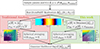 |
Fig. 1. Flowchart comparing the current state-of-the-art inference pipeline (left side) with this work (right side). In current state-of-the-art pipelines, we use a single realisation of the ICs to estimate the mean 1D 21 cm PS. Moreover, the simulated 1D PS is computed by spherically averaging over different wave modes than those used to compute the observed 1D PS. In this work, we account for sample variance by applying 21cmPSDenoiser a score-based diffusion model trained to estimate the mean 21 cm PS from a single realisation. We also account for 21 cm PS anisotropy by averaging the 2D PS only over modes above μmin = 0.97, the region of 2D PS that is closest to where current 21 cm PS instruments observe. Applying a cut in μmin significantly exacerbates the problem of sample variance and would not be practical without the use of 21cmPSDenoiser. |
2.1. Forward-modelling the 21 cm signal
A single forward model of the cosmic 21 cm signal consists of the following steps:
-
Sample astrophysical and cosmological parameters. For a given set of cosmological parameters, generate ICs (e.g. a Gaussian random field sampled from a PS) creating a realisation of the linear matter density and velocity fields.
-
Evolve densities and velocities to lower redshifts (e.g. via second-order Lagrangian perturbation theory; Scoccimarro 1998).
-
Assign galaxy properties to the dark matter halos according to the sampled astrophysical parameters (e.g. via semi-empirical relations; Park et al. 2019).
-
Compute corresponding inhomogeneous radiation fields and their role in heating and ionising the intergalactic medium.
-
Calculate the corresponding 21 cm brightness temperature at each cell and redshift, (x, z) (e.g. Madau et al. 1997; Furlanetto 2006; Pritchard & Loeb 2012):
![Mathematical equation: $$ \begin{aligned} T_{\rm b}(\boldsymbol{x}, z)&= \frac{T_{\rm S} - T_{\rm R}}{1+z}(1-e^{\tau _{21}})\\ \nonumber&\approx 27 \ x_{\rm HI} (1 + \delta _{\rm b}) \left( \frac{\Omega _{\rm b} h^2}{0.023}\right) \left( \frac{0.15}{\Omega _{\rm m} h^2} \frac{1+z}{10}\right)^{1/2} \ \mathrm{mK} \\ \nonumber&\times \left( \frac{T_{\rm S} - T_{\rm R}}{T_{\rm S}}\right) \left[ \frac{\partial _r v_{\rm r}}{(1+z)H(z)}\right], \end{aligned} $$](/articles/aa/full_html/2025/11/aa56449-25/aa56449-25-eq12.gif) (2)
(2)where τ21 is the 21 cm optical depth of the intervening gas, and TS and TR are the spin and background temperatures, respectively8. xHI is the fraction of neutral hydrogen,
 is the baryon overdensity, ∂rvr is the baryon peculiar velocity gradient along the line of sight, H(z) is the Hubble parameter at redshift z, and Ωm and Ωb are the mass densities of cold dark matter and baryons, respectively.
 -
Compute a summary statistic from the 21 cm brightness temperature light cone, in order to compare it to the same summary of the observation. Currently all9 analyses use the spherically averaged 1D 21 cm PS as a summary:
 (3)
(3)where
 is the conjugate of the Fourier transform of the 21 cm brightness temperature at redshift z and wave mode,
 ![Mathematical equation: $ k{\prime}[\mathrm{Mpc}^{-1}] = \sqrt{k_x^2+k_{\mathit{y}}^2+k_z^2} = \sqrt{k_\perp^2+k_\parallel^2} $](/articles/aa/full_html/2025/11/aa56449-25/aa56449-25-eq16.gif) , for a spherical average and cylindrical average at sky-plane mode k⊥ and line-of-sight mode k∥, respectively. δD is the Dirac delta function, and Δ212(k, z) in mK2 is the dimensionless 21 cm PS per logarithmic wave mode interval.
, for a spherical average and cylindrical average at sky-plane mode k⊥ and line-of-sight mode k∥, respectively. δD is the Dirac delta function, and Δ212(k, z) in mK2 is the dimensionless 21 cm PS per logarithmic wave mode interval.
Once the forward model is compressed into a summary statistic such as the 21 cm PS, it is compared to the observation by evaluating the likelihood.
2.2. Evaluating the likelihood on the 21 cm PS
For complex physical models such as the 21 cm signal, the likelihood function is analytically intractable. As such, all current inferences assume a Gaussian functional form10 as defined in Eq. (1). Assuming a diagonal variance and approximating the mean 21 cm PS with a single realisation Δ21, i2 can produce a large bias in the resulting posterior for high S/N data (e.g. over 5σ as seen from Figure 5 in Prelogović & Mesinger 2023 ).
Another common approximation of the traditional analysis is that the 1D PS is computed by averaging the amplitudes of all wave modes in a given k-bin. However, as shown in Figure 2, the footprint of 21 cm interferometers in cylindrical (2D) k-space can be very different from the corresponding footprint of the forward model.
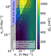 |
Fig. 2. Cylindrically averaged (2D) 21 cm PS as a function of line-of-sight modes k∥ and sky-plane modes k⊥. The colour map shows the PS amplitude calculated from a slice through a single simulated light cone centred at z = 9. The simulation box has a side length of 300 cmpc and was generated with 21cmFASTv3. The blue hashed area is the HERA EoR window. The dashed cyan line is the horizon limit and the solid black line is the horizon limit with a 300 ns buffer added to it to account for additional foreground leakage (see HERA Collaboration 2023). The solid red line is drawn at a value of μmin = 0.97, where μmin = cos θ, and |

The cylindrical k-space available to interferometers is limited by a combination of foregrounds, instrument layout, and dish size. The distribution of baselines limits the accessible angular scales. Foregrounds dominate in the regime of low k∥, since they are spectrally smooth. The chromatic instrument response, however, causes the foregrounds to leak out into a ‘wedge’-like region in 2D k-space (e.g. Parsons et al. 2012; Liu et al. 2014a,b). As a result, ‘clean’ EoR measurements are performed outside (or near the boundary) of the wedge (c.f. blue shaded region in Figure 2). The cylindrical k-space available to forward models is limited by the need to resolve relevant sources and sinks and the corresponding physical processes. This means that cell sizes of physics-rich simulations cannot be much larger than ∼1 Mpc. On the other hand, needing to compute thousands of forward models in a reasonable time limits the box sizes to approximately a few hundred Mpc. Therefore, forward models typically span wave modes of 1 ≲ k/Mpc−1≲few × 0.01.
This discrepancy between the k-space footprint of observations and simulations is problematic because the 21 cm PS is anisotropic due to RSDs and the light cone evolution along the line-of-sight axis. This issue can be avoided by cropping the forward-modelled 2D PS to the k-space region closest to that of the observation (e.g. the region above the red line in Figure 2). However, cropping out modes exacerbates the sample variance problem at large scales as it significantly reduces the number of modes available to perform theaveraging.
In this work we introduce 21cmPSDenoiser (right branch of Figure 1) to mitigate sample variance: after a forward model is computed, the resulting 2D PS realisation is passed through our neural network (NN) that produces an accurate estimate of the mean 21 cm PS. Mitigating sample variance with 21cmPSDenoiser allows us to also take into account the 21 cm PS anisotropy: we introduce a cut in cylindrical PS space where we exclude all Fourier modes below μmin = 0.97, marked by a red line in Figure 2, where μmin = cos θ, and  . Introducing this cut significantly reduces the bias due to PS anisotropy (e.g. Pober 2015). Restricting the k-space footprint comes at the cost of further increasing sample variance and thus further increases the benefits of using21cmPSDenoiser.
3. Mitigating sample variance with score-based diffusion
In this section, we first introduce the training database and the NN architecture of 21cmPSDenoiser. We then evaluate the NN on a separate database of test samples and comment on its performance.
3.1. Simulated dataset
We built a training database with over one hundred light cone realisations (i.e. IC samples) for each set of astrophysical parameters. We simulated a light cone with 21cmFAST v311 (Mesinger & Furlanetto 2007; Mesinger et al. 2011; Murray et al. 2020) and use ‘The Ultimate EoR Simulation Data AnalYser’ (tuesday)12, a wrapper around powerbox13 (Murray 2018), to calculate the 2D PS. Our simulation boxes are 300 cmpc on a side, with a cell size of 1.5 cmpc. This is characteristic of the cosmological simulations used to interpret 21 cm observations (e.g. Muñoz et al. 2022; Nunhokee et al. 2025; Ghara et al. 2025).
We varied five astrophysical parameters θastro = (fesc, 10, f*, 10, Mturn, LX, < 2keV/SFR, E0), introduced in Park et al. 2019:
-
fesc, 10, the amplitude of the power-law describing the ionising escape fraction fesc(Mh)∈[0, 1] to halo mass relation fesc(Mh) = fesc, 10(Mh/M10)αesc, where M10 = 1010 M⊙ and the index αesc = 0.5 was fixed (e.g. Paardekooper et al. 2015; Kimm et al. 2017; Lewis et al. 2020);
-
f*, 10, the amplitude of the stellar-to-halo mass relation (SHMR) normalised at M10. Similarly to the ionising escape fraction, the faint-end SHMR is described by a power-law whose index we fix to α* = 0.5 (e.g. Mirocha et al. 2017; Munshi et al. 2017, 2021);
-
Mturn[M⊙], the characteristic halo mass scale below which the abundance of galaxies becomes exponentially suppressed to account for inefficient star formation in low-mass halos (e.g. Hui & Gnedin 1997; Springel & Hernquist 2003; Okamoto et al. 2008; Sobacchi & Mesinger 2013; Xu et al. 2016; Ocvirk et al. 2020; Ma et al. 2020);
-
![Mathematical equation: $ \log_{10} \frac{L_{\rm X, < 2\,keV}}{{\rm SFR}} \left[\frac{{\rm erg\,s}^{-1}}{{\rm M}_\odot\,{\rm yr}^{-1}}\right] $](/articles/aa/full_html/2025/11/aa56449-25/aa56449-25-eq19.gif) , the X-ray luminosity escaping the galaxies is modelled as a power-law in energy, which we normalised with the soft-band (i.e. < 2 keV) X-ray luminosity per unit star formation rate (SFR). We fixed the power law index of the X-ray spectral energy distribution to αX = 1.0 (e.g. Fragos et al. 2013; Pacucci et al. 2014; Das et al. 2017);
, the X-ray luminosity escaping the galaxies is modelled as a power-law in energy, which we normalised with the soft-band (i.e. < 2 keV) X-ray luminosity per unit star formation rate (SFR). We fixed the power law index of the X-ray spectral energy distribution to αX = 1.0 (e.g. Fragos et al. 2013; Pacucci et al. 2014; Das et al. 2017); -
E0[eV], minimum energy of X-ray photons capable of escaping their host galaxy;
Well-established observations already provide some constraints for fesc, f*, and Mturn. To build our training set, we sampled these three parameters from a posterior informed by UV luminosity functions (LFs) from Hubble (Bouwens et al. 2015, 2016; Oesch et al. 2018), the Thomson scattering cmB optical depth from Planck (Planck Collaboration 2020; Qin et al. 2020), and the Lyman forest dark fraction (McGreer et al. 2015). The resulting posterior is shown in green in Figure 8 of Breitman et al. 2024). For the remaining two parameters, we sampled a flat prior over log10LX, < 2 keV/SFR ∈ [38, 42] and E0 ∈ [200, 1500] (e.g. Furlanetto 2006; HERA Collaboration 2023).
The database used for training and validation consists of roughly 900 parameter combinations with an average of roughly 100 realisations per parameter set. This amounts to ∼90 k total light cones. For each light cone realisation, we calculated the 2D PS on cubic chunks over 40 redshift bins z ∈ [5.5, 35]. We re-binned the 2D PS to be linearly spaced in log scale in both sky-plane and line-of-sight modes. To minimise the number of empty bins while keeping the 2D PS dimensions in powers of two that are more convenient for the NN, we chose 32 k⊥ bins and 16 k∥ bins. Due to the re-binning of k⊥ into log-spaced bins, we ended up with three empty bins: the second, fourth, and fifth. We filled the power in those bins by interpolating with SciPy (Virtanen et al. 2020), which can produce artefacts in individual realisations (e.g. see horizontal bright yellow stripes in the top left plot of Figure 4). These artefacts, however, did not affect the mean 21 cm PS as they are another effect of sample variance and get averaged out. Since the NN is redshift-agnostic, the final database consisted of about 3.6M 2D PS. This database was then split into 90% training set with 10% left for the validation. The test set was made separately from the training and validation sets and is described in Section 3.3.
We pre-processed the data by applying min-max normalisation on the log of the 21 cm PS and then rescaling it to[ − 1, 1]:
 (4)
(4)
The minimum and maximum are each a scalar obtained over the entire training and validation databases.
3.2. Denoiser architecture and training
We interpret sample variance as a form of non-uniform, (mildly) non-Gaussian (e.g. Mondal et al. 2015; Shaw et al. 2019) ‘noise’ added to the target mean PS. Obtaining the mean cylindrical PS from a single (‘noisy’) realisation is thus akin to denoising a 2D image. This is a common task in image processing, for which machine learning is known to outperform traditional methods (e.g. Kawar et al. 2022) such as Gaussian filter smoothing or principal component analysis. The idea is to train a NN to find a smooth function that interpolates through fluctuating data points, with minimal loss of intrinsic scatter. In our usage case, the small scales with negligible sample variance (see top-right corner of Figure 2) can serve as anchor to the NN prediction of the mean for the noisy larger scales (see bottom-left corner of Figure 2).
Here, we adopted a state-of-the-art NN architecture for image generation that has also been shown to excel at image denoising (e.g. Kawar et al. 2022): a score-based diffusion generative model (e.g. Sohl-Dickstein et al. 2015; Song & Ermon 2019, 2020, 2019; Ho et al. 2020; Song et al. 2020). In Figure 3 we illustrate the general idea behind diffusion models:
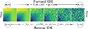 |
Fig. 3. Illustration of the forward and backward diffusion processes used in 21cmPSDenoiser. The forward process adds noise to a mean 21 cm 2D PS sampled from the data distribution (leftmost panel), transforming it into a pre-defined Gaussian prior distribution (rightmost panel). This allows us to then write the reverse process that allows us to sample the Gaussian prior and generate a mean 2D PS, conditioned on the input realisation of the 2D PS. |
-
Left to right: the forward diffusion process can be interpreted as a continuous noise-adding stochastic process where we corrupt a mean 21 cm PS from the training set with Gaussian noise with increasing variance according to a chosen variance schedule until it is transformed into a sample from a standard normal prior distribution. This stochastic process can be written as a solution to a stochastic differential equation (SDE):
 (5)
(5)where
 is the diffused data (i.e. a 2D PS) at a given time in the diffusion process, t ∈ [0, T], with x(0) denoting a sample from the data distribution of mean 2D PS and x(T) a sample from the Gaussian prior. w is a Wiener process (also known as Brownian motion). The drift function f(x, t) and the diffusion coefficient g(t) are hyperparameters of our model. We chose the most standard drift function and diffusion coefficient leading to the variance preserving SDE (Song et al. 2020), which is the continuous-time limit of the variance schedule in the denoising diffusion probabilistic model (DDPM; Ho et al. 2020).
 -
Right to left: in order to generate new data samples from Gaussian prior samples, we needed to reverse the forward process, which can be done by solving the following SDE (Anderson 1982):
![Mathematical equation: $$ \begin{aligned} d\boldsymbol{x} = \big [\boldsymbol{f}(\boldsymbol{x},t) - g(t)^2 \nabla _{\boldsymbol{x}} \log P_{t} (\boldsymbol{x}|\boldsymbol{x}_i) \big ] dt + g(t) d\boldsymbol{\overline{w}}, \end{aligned} $$](/articles/aa/full_html/2025/11/aa56449-25/aa56449-25-eq23.gif) (6)
(6)where the only unknown is the score function ∇xlog Pt(x|xi) of the probability density function (PDF) P of the data x (in this case, the 2D PS means) explicitly conditioned on a 2D PS realisation xi in addition to the continuous diffusion time index t. At t = 0, the entire procedure boils down to mapping any input 2D PS realisation to its corresponding mean 2D PS.
In order to solve the reverse SDE written above and generate a mean 2D PS from a given 2D PS realisation, we trained a NN to learn the score function. Here, we use a U-Net autoencoder architecture14 similar to Ho et al. 2020 implemented with PyTorch (e.g. Paszke et al. 2019. U-Nets have been developed for image segmentation as they are efficient in recognising local information in images over a range of scales (Ronneberger et al. 2015). We trained the NN with the continuous-time generalisation of the standard DDPM loss function (see Eq. (7) in Song et al. 2020) with the Adam optimiser (Kingma & Ba 2017).
During training, the NN learned to accurately predict the score for various levels of noise. It is precisely due to this training method that score-based diffusion models, and diffusion models in general, perform very well on tasks such as image denoising: the denoising task itself is part of the training process. Once the NN was trained to accurately predict the score for varying noise levels indexed by t, we were able to generate new mean 2D PS samples given one 2D PS realisation by solving this reverse-time SDE. Since our goal was to use the score-based diffusion model as part of an inference pipeline, we solved the reverse SDE via the probability-flow ODE method (Song et al. 2020). This algorithm modestly sacrifices accuracy for a significant speed increase. In order to average over the network error, our final estimate of the mean 2D PS corresponds to the median obtained over 200 samples (i.e. draws from the prior) from 21cmPSDenoiser for a given input. For these choices, we obtained a mean 2D PS estimate from a single realisation in ∼6 s on a V100 GPU, which reduces to ∼2 s when taking advantage of GPU vectorisation by denoising multiple realisations at once.
3.3. Performance on the test set
The test set is composed of 50 parameter combinations distinct from the parameters in the training and validation sets with about 200 realisations per parameter and 40 redshift bins for a total of 400k 2D PS. Since the test set is significantly smaller than the training set, we could afford to have a larger number of realisations for each parameter, allowing a more accurate estimate of the true, target mean PS. We assessed the performance of 21cmPSDenoiser using the fractional error (FE) evaluated on a random 40k batch of the test set:
 (7)
(7)
where Δ21, test2 is the target mean PS, obtained by averaging over 200 realisations per parameter combination, and Δ21, μ2 is a mean 2D PS estimate such as from 21cmPSDenoiser. We note that to avoid the FE exploding at small power, we floored the denominator to 0.01 mK2, which is an order of magnitude smaller than the accuracy of the 21cmFAST simulator itself (e.g. Mesinger et al. 2011; Zahn et al. 2011). We calculated the FE for each realisation from each parameter combination and redshift.
In Figure 4 we illustrate the impact of sample variance using a single PS realisation (left column) and after applying 21cmPSDenoiser (right column). This realisation was chosen from the θmock parameter vector in the test set. This parameter combination is consistent with the most recent constraints from observations such as the Lyman-α forest (e.g. Qin et al. 2025 and UV LFs; Bouwens et al. 2015, 2016; Oesch et al. 2018); see Section 6.1 for more details. The top row shows the cylindrical PS realisation at z ∼ 6.1 and the resulting mean estimate obtained from 21cmPSDenoiser using the realisation shown on the left. In the middle row, we compare them to the test set mean PS via the FE where  on the right and Δ21, μ2 = Δ21, i2 on the left. The plotted PS realisation has a median FE very close to that of the entire test set for 21cmPSDenoiser (see top half of Table 1) and can therefore be considered representative. We see that the fractional sample variance error on large scales can be reduced by over an order of magnitude by calling 21cmPSDenoiser.
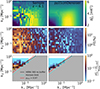 |
Fig. 4. Top row: PS sample (left) and NN mean estimate from this same PS sample as input (right). Middle row: FE with respect to the mean PS obtained from an ensemble average of about 200 PS realisations for the sample (left) and 21cmPSDenoiser (right). Bottom row: error as a fraction of the HERA noise level at the same redshift for the sample (left) and for the 21cmPSDenoiser (right). |
Median and 68 % CL on the FE and AE of a ∼40k random batch from the test set over 40 redshift bins ∈[5.3, 33].
To put these errors into better perspective, the bottom row shows the square root of the squared deviation from the test set mean normalised by realistic HERA sensitivities (see Section 6 for more details). The left plot on the bottom row shows that the deviation from the mean due to sample variance is comparable to or larger than HERA sensitivity at large scales, k ∼ 0.1 Mpc−1, and remains significant (∼10%) up to much smaller scales, k ∼ 0.5 Mpc−1. The right plot shows that applying 21cmPSDenoiser reduces sample variance enough that the residual deviation from the mean is very small (≲1%) in comparison to the instrument sensitivity.
In Figure 5 we show the median of the FE computed from ∼2.5 k test samples at redshift z ∼ 11.4. In the left plot, we evaluate the FE over the PS realisations while in the right plot we evaluate it over the 21cmPSDenoiser mean estimate. We can see that when taking the median over ∼2.5 k test samples, individual bins can deviate from the mean by over 30% on large scales and that 21cmPSDenoiser reduces this deviation down to ∼3%. Individual bins from single PS realisations as shown in Figure 4, on the other hand, can deviate from the mean by over 50% on large scales, which gets reduced down to ∼5% by 21cmPSDenoiser. The striped pattern in the right plot occurs due to the binning scheme, where certain bins have more samples (and thus less sample variance) than others.
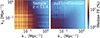 |
Fig. 5. Median FE on ∼2.5 k test samples at redshift z ∼ 11.4. The left plot evaluates the FE directly on the PS realisations, while the right plot evaluates it on the output from 21cmPSDenoiser. The striped pattern in the right plot occurs due to the binning scheme, where certain bins have more samples (and thus less sample variance) than others. |
4. Comparing 21cmPSDenoiser to fixing and pairing
In this section we compare our results against F&P (e.g. Angulo & Pontzen 2016; Pontzen et al. 2016; Acharya et al. 2024), the benchmark technique for mitigating sample variance. F&P involves pairing a simulation to a given fixed simulation by reversing the sign of the initial matter overdensity field ,  , such that δpaired(k) = − δfixed(k), for every wave mode k. Each mode whose amplitude is above the mean initial matter PS in one simulation has a counterpart whose amplitude is equally below the mean in the other simulation. Averaging F&P simulations by construction would yield the mean initial matter PS for the chosen cosmology, but it has also been shown to give a good estimate of the mean PS of evolved fields, including galaxy and line intensity maps (e.g. Angulo & Pontzen 2016; Pontzen et al. 2016; Villaescusa-Navarro et al. 2018).
Nevertheless, F&P has two main shortcomings: (i) it is still computationally expensive, as it doubles the cost of the inference; and (ii) due to non-linear evolution of the 21 cm signal, F&P becomes less effective with decreasing redshift, which is where current instruments are most sensitive (Acharya et al. 2024).
We built a database of 20 F&P pairs for each of the 50 parameter combinations in the test set. In Figure 6 we compare the FE for the F&P method (purple / left violins) with 21cmPSDenoiser (black / right violins). We performed this comparison on PSs with mean power greater than 0.01 mK2 for ∼17 k samples cropped at μmin = 0.97. We can see that 21cmPSDenoiser has median FE that is about 5% lower than F&P across most redshifts15.
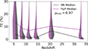 |
Fig. 6. PDFs of the FE as a function of redshift for F&P (purple / left violins) and 21cmPSDenoiser (black / right violins) computed on PS modes above μmin > 0.97 (see red line in Figure 2). The distributions were generated using the 50 parameter samples comprising our test set. |
We summarise the results in Table 1, where we show the median and 68% confidence limits (CLs) of the FE and absolute error (AE) of: (i) individual samples; (ii) the mean estimated from F&P; and (iii) the mean estimated from 21cmPSDenoiser. The top half of the table shows the FE and AE evaluated over all cylindrical modes, while the bottom half does so over the region above μmin = 0.97. We see that 21cmPSDenoiser results in a FE that is a factor of ∼2.5 (∼4) smaller than F&P over all k-space (μmin = 0.97 region). Additionally, unlike F&P, using 21cmPSDenoiser in inference comes at essentially no additional computational cost.
We note that there are cases where 21cmPSDenoiser can produce an output that is farther away from the mean PS than even the noisy sample it was given as input. However, such cases are rare, as demonstrated in this section. In general, the denoiser is more likely to fail when the input is uninformative, as may happen when the neutral fraction is very low and the 21 cm PS has little power. As such, we generally recommend applying 21cmPSDenoiser on signal with neutral fraction ≳0.05 or with mean power ≳10−2 mK2 in the input realisation.
5. Application to other simulators
As motivated in the introduction, one benefit of our approach is that, unlike emulation, it is model- and simulator-agnostic. 21cmPSDenoiser can in principle operate on any 2D PS, regardless of what model or simulator was used to make it. In this section, we test 21cmPSDenoiser on hydrodynamic radiative transfer (RT) simulations from Acharya et al. 2024. Similar to THESAN (e.g. Garaldi et al. 2022; Kannan et al. 2022), these simulations implement moving mesh hydrodynamics with AREPO (e.g. Springel 2010; Weinberger et al. 2020), and RT of ionising photons with AREPO-RT (e.g. Kannan et al. 2019). Furthermore, as they lack Lyman band and X-ray RT, these simulations make the simplifying assumption of a homogeneously saturated spin temperature: TS ≫ TR in Eq. (2). These hydro RT simulations are therefore very different from those used in training 21cmPSDenoiser, both in terms of the source model and the simulator.
From Acharya et al. (2024), we have a total of 40 simulations varying ICs for one parameter set, where five of these also have an additional paired simulation. We post-processed the coeval cubes from these simulations into light cones using tools21cm16 (Giri et al. 2020). These resulting light cones have a resolution of 0.373 cmpc and a box size of 95.5 cmpc. 21cmPSDenoiser, however, is not capable of generalising to a different k-space footprint or resolution. As such, we calculated the 2D PS from these light cones with the goal to match the 2D PS from the training database as closely as possible. This involves taking these light cones and first down-sampling them by a factor of four so that they have roughly the same resolution as the 21cmFAST simulations in the training set. Next, we calculated the 2D PS on the same k-space binning as the training set. However, since these boxes are about three times smaller, this leaves many large-scale mode bins empty. We padded these large-scale bins by copying over the power from the closest non-empty bin at smaller scales. This padded 2D PS is then passed to 21cmPSDenoiser17.
In Figure 7 we show the de-noised PS on the right, corresponding to the single hydro RT realisation input shown on the left. Each row corresponds to a different realisation. We note that in all plots, we crop the k-space footprint to only include the non-empty bins (i.e. we do not consider the padded bins as we have no larger hydro RT simulations against which to compare them). We note that with only 35 realisations and 5 F&P pairs, the estimate of the true target mean is not as accurate as it is for the test set, where we have ∼200 realisations per parameter. As a consequence, the performance of the NN reported in this section is not as accurate as in previous sections.
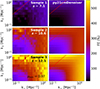 |
Fig. 7. 21 cm PS realisations from a hydro RT simulation (left column) and the corresponding mean estimate (right column) obtained after passing the realisation on the left to 21cmPSDenoiser (which was only trained on 21cmFAST). Each row corresponds to different ICs and redshift. |
We see from Figure 7 that 21cmPSDenoiser is flexible enough to mitigate sample variance on 21 cm PSs from different astrophysical models and different simulators. We confirm this by looking at Figure 8, where we plot the FE of the samples shown in Figure 7. The mean PS above μmin = 0.97 is recovered to an median accuracy of about ∼4% over all redshifts and PS realisations for the denoiser, while sample variance introduces a median deviation of about ∼10% in the same region. We note that the samples shown have an average FE at the redshift plotted that is slightly above the average FE over all available realisations. Figure 8 also shows that on the largest and smallest scales, 21cmPSDenoiser tends to under-predict the mean power: a behaviour not seen in the test set cases. It is reasonable, however, that the out-of-distribution performance is weaker than that seen for the test set. One could further improve the generalisation of 21cmPSDenoiser by fine tuning it on 21 cm PSs from different models and simulators.
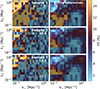 |
Fig. 8. FE on the 21 cm PSs shown in Figure 7. We caution that the mean PS is estimated from a relatively small number of realisations (35 unpaired ICs plus 5 pairs of ICs). |
6. Application to inference
In this section, we test the performance of 21cmPSDenoiser by performing inference on a HERA mock observation. We compare the traditional state-of-the-art inference pipeline with the improvements introduced in this work (i.e. left vs right of Figure 1).
6.1. Mock HERA observation
We chose the mock parameter set θmock with (log10fesc, 10, log10f*, 10, Mturn, log10LX, < 2 keV/SFR, E0) = (−1.23, −1.36, 8.26, 40.59, 1.40 keV) out of the 50 parameter sets available in the test set as it has an EoR history that is consistent with that inferred from Lyman-α forest data (Qin et al. 2025), and matches UV LFs at z = 6–10 (Bouwens et al. 2015, 2016; Oesch et al. 2018). In addition to thermal variance from the instrument, an observation of the 21 cm PS is subject to cosmic variance due to the fact that there is only one Universe with its own set of ICs to observe, i.e. we do not observe the expectation value of the 21 cm PS (over all possible observable universes), but rather a realisation with a finite volume. Cosmic variance has the most effect at the largest scales of an observation as there are fewer Fourier modes to be observed given the finite size of the observable Universe. However, since HERA observations span a much larger field than our forward models, cosmic variance on the scales of the simulation is negligible. Our mock cosmic signal was therefore taken to be the mean 21 cm PS, averaged over the 200 realisations of ICs for θmock. As our observational summary statistic, we spherically averaged this mean cylindrical PS above μmin = 0.97, mimicking the observational footprint (c.f. Figure 2), obtaining the 1D PS at z = 5.6, 6.1, 6.9, 7.9, 9.1, 10.4, 10.8, 16.8, and 22.7.
We used 21cmSense (Pober et al. 2013, 2014; Murray et al. 2024) to forecast the sensitivity for two full seasons of phase II HERA observations where we observed for 94 nights per season for a total of ∼2256 integration hours (see HERA Collaboration 2023 and the appendix in Breitman et al. 2024 for more details). The forecast assumed that the number of observed hours is the same in both seasons. The only difference between the two seasons was the number of operating antennas that increased from 140 in the 2022–2023 season to 180 in the 2023–2024 season. To combine the two observations, we summed the total integration times as well as the uv coverage of both seasons. We then used these combined integration time and uv-coverage to obtain the thermal variance of the HERA instrument over both seasons. We also included the cosmic variance of the observation in the error budget, adding it to the thermal noise in quadrature:  , where we refer to σsens as the sensitivity.
After this procedure, we are left with HERA mock 1D 21 cm PSs at all redshifts, together with the associated sensitivities. In Figure 9 we plot the mock observation at z = 10.8 as the pink points with 1σ error bars. In orange, we show different PS realisations with θ = θmock, where all modes (i.e. μmin = 0) of the 2D spectrum have been included in the average, instead of the modes above μmin = 0.97 used for the mock. We see that there is significant scatter between the realisations at the largest scales even when we include all available modes. Aside from the realisation-to-realisation scatter between the orange curves, we find that they are biased by a factor of ∼3, revealing the effects of anisotropy when the correct μmin is neglected18.
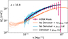 |
Fig. 9. Spherically averaged 21 cm PSs at z = 10.8 corresponding to a parameter vector in our test set, θmock. Pink points and error bars correspond to a mock ∼2256 h observation with HERA (see text for details). In orange, we plot different realisations, varying ICs at a fixed θmock, but spherically averaging the 2D PS down to μmin = 0, as is commonly done when forward-modelling. In blue, we plot these realisations but instead averaging only down to μmin = 0.97 to account for the HERA footprint in cylindrical space (see red line in Figure 2). Excising low μ modes removes the bias seen in the orange curves, but dramatically increases the sample variance. The dashed black line corresponds to the output of 21cmPSDenoiser from a single 2D PS realisation, averaged down to μmin = 0.97. We see that applying 21cmPSDenoiser mitigates both the bias and the sample variance. |
In blue, we show PS realisations also with θ = θmock, but now averaging over only the modes ‘observed’ in the mock with μmin = 0.97. Unlike the orange curves, these do not display a significant bias with respect to the mock data. However, limiting the modes over which to perform the averaging results in substantial sample variance at small k. The level of sample variance is well in excess of the observational error bars and we thus expect it to limit the inferred parameter constraints (as we confirm below).
The dashed black line shows the mean PS obtained from 21cmPSDenoiser derived from a single realisation. Similarly to the blue curves, this de-noised PS is averaged only over modes above μmin = 0.97.
The denoised PS agrees very well with the mock data, with no obvious bias and a dramatic reduction of the effects of sample variance (seen by the reduction in bin-to-bin variance) compared with the blue curves.
6.2. Inference setup
To quantify the qualitative trends seen in Figure 9, we used our HERA mock observation to perform inferences under different approximations:
-
(i)
No 21cmPSDenoiser and no μmin cut – this corresponds to the current approach of spherically averaging the forward-modelled 2D PS down to μmin = 0 using a single realisation of the ICs (c.f. orange curves in Figure 9);
-
(ii)
No 21cmPSDenoiser with μmin = 0.97 cut – this also uses a single realisation of the 2D PS, but averages down to the same μmin = 0.97 as is used for the mock data (c.f. blue curves in Figure 9);
-
(iii)
21cmPSDenoiser with μmin = 0.97 cut – this uses a single realisation of the 2D PS passed to 21cmPSDenoiser to obtain the mean 2D PS, before averaging down to the correct μmin = 0.97 (c.f. dashed black curve in Figure 9).
In all of the inferences, the likelihood is constructed by multiplying individual likelihoods based on four observables:
-
(i)
21 cm 1D PS: following Figure 1, we forward-modelled the 2D PS Δ21, i2(k⊥, k∥, z). We then estimated the mean PS:
 We then averaged the mean 2D PS to 1D, weighting each 2D bin by the number of 3D Fourier modes it contains, Nk:
 (8)
(8)where 𝒦i is the set of
 19. We then applied a window function W (e.g. Liu et al. 2014a,b; Gorce et al. 2023) calculated with hera-pspec20 to the forward-modelled 1D PS. The window function converts the forward-modelled 21 cm PS to an observed PS by including instrumental effects such as the chromaticity of the baselines and the beam, especially affecting large-scale modes. The likelihood function is a Gaussian:
 (9)
(9)summed over all frequency bands f and k-bins, where the total variance σ2 includes the sensitivity of the mock observation σsens2 and a contribution from the forward model σfm2 coming from either Poisson sample variance or the mean NN error following
 (10)
(10) (11)
(11) -
(ii)
UV LFs: we included UV LFs at z = 6, 7, 8 and 10 based on Hubble data (Bouwens et al. 2015, 2016; Oesch et al. 2018) as in previous works (e.g. HERA Collaboration 2022; Breitman et al. 2024). This likelihood function was also assumed to be Gaussian.
-
(iii)
Thomson scattering optical depth to the cmB: we included a Gaussian likelihood centred around
 based on the median and 68% credible interval (CI) from the posterior obtained in Qin et al. 2020 from their re-analysis of Planck Collaboration 2020 data.
 -
(iv)
Lyman forest dark fraction: this term compares the proposed model’s global neutral fraction at z = 5.9 with the upper bound
 at 68% CI obtained with the model-independent quasi-stellar object dark fraction method (McGreer et al. 2015). The likelihood function is unity if the proposed global neutral fraction is below the upper bound at z = 5.9, then it decreases as a one-sided Gaussian for higher values of
  .
.
For computational convenience, we fixed E0 and LX to the true values in θmock and performed the inference over the remaining three astrophysical parameters for which we assumed flat priors over the following ranges: (i) log10f*, 10 ∈ [ − 2, −0.5]; (ii) log10fesc, 10 ∈ [ − 3, 0]; and (iii) Mturn[M⊙]∈[8, 10].
We ran the inferences with the 21cmMC21 (e.g. Greig & Mesinger 2015, 2017, 2018) package using the MultiNest (e.g. Feroz et al. 2009)22 sampler. Each inference required about 15k likelihood evaluations. In the following section, we show and discuss the posterior from each of these inferences.
6.3. Inference results
In Figure 10 we show the marginal posteriors of our three inferences, together with the true values, θmock (marked in pink). In orange, we show the posterior for inference (i). As foreshadowed by the orange curves in Figure 9, we see that the posterior is indeed biased, due to the mismatch of the 2D PS footprints of the observation and forward model. The bias is at the level of ∼10% in the inferred ionising escape fraction and stellar fraction parameters. More dramatic, however, is the overconfidence of the biased posteriors, with the true values being outside ∼10σ for both f*, 10 and fesc, 10.
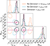 |
Fig. 10. 1D and 2D marginal posteriors from three inferences described in the text: (i) traditional state-of-the-art analysis using a single IC realisation and spherically averaging the 2D PS down to μmin = 0 (orange); (ii) using a single IC realisation but spherically averaging the 2D PS down to the same μmin = 0.97 used for the mock data (blue); and (iii) applying 21cmPSDenoiser to a single realisation in order to mitigate sample variance followed by the μmin cut to mitigate PS anisotropy (black). The 2D contours show 95% CIs. The pink lines show the true parameters θmock. |
In blue, we show the posterior for inference (ii). Again, as foreshadowed by the correspondingly coloured curves in Figure 9, this posterior is unbiased; however, it is notably wider than the posterior for inference (iii), shown in black. This highlights the impact of sample variance. Applying 21cmPSDenoiser to a realisation of the 2D PS during inference tightens the inferred 1D marginal parameter constraints by ∼50%. While these quantitative results are HERA-specific due to our HERA-motivated choice of μmin, we expect the qualitative trends to hold for any instrument.
7. Conclusion
In this work, we studied the consequences of two common approximations made on the 21 cm PS likelihood in Bayesian inference problems:
-
(i)
Replacing the 21 cm PS mean with a sample from a single realisation; and
-
(ii)
Averaging the 3D Fourier modes within a k bin over all orientations, instead of matching those actually observed by 21 cm PS experiments.
In order to relax both of these assumptions, we developed 21cmPSDenoiser, a score-based diffusion model that provides an estimate of the mean cylindrical 21 cm PS given a single realisation. Unlike emulators, 21cmPSDenoiser is not tied to a particular model or simulator since its input is a (model-agnostic) realisation of the 2D 21 cm PS. 21cmPSDenoiser outperforms state-of-the-art analytical approaches such as F&P, the benchmark technique for sample variance mitigation. Individual 2D PS realisations can deviate from the mean by over 50% at scales relevant to current interferometers. 21cmPSDenoiser reduces this deviation to ∼2%, over a factor of 2 better than F&P, and at almost no additional cost (∼2 s per iteration). Moreover, we tested 21cmPSDenoiser on 21 cm PSs from a completely different simulator and astrophysical model. We find that it produces reasonable PSs and produces a mean estimate that is ∼2.5 times more accurate than the 2D PS realisation itself above μmin = 0.97, the region of cylindrical PS space most relevant to current observations.
We tested 21cmPSDenoiser by applying it in a realistic inference context. First, we simulated a realistic HERA mock 21 cm PS observation with 21cmSense. Then, we ran a set of three inferences: (i) a classical inference such as previous state-of-the-art inferences; (ii) an improved inference where we solved only the first issue mentioned above; and (iii) where we solved both issues. We find that inference (i), the typical state-of-the-art inference method, produces a highly overconfident and biased posterior with a bias of over 10σ for two of the three parameters. In inference (ii), we cropped the k-space of our cylindrical 21 cm PS closer to that of observations by applying a cut at μmin = 0.97, and, as expected, we obtained an unbiased but wider posterior. Finally, we applied both 21cmPSDenoiser and the cut at μmin = 0.97 in inference (iii), and obtained an unbiased posterior that is on average 50% narrower for each parameter. We thus explicitly show that 21cmPSDenoiser would benefit HERA data analysis in the very near future. Our proposed method, however, would also be highly applicable for upcoming experiments such as the SKA, especially for its earliest observation modes that are limited to substation layouts of, for example, 12 m or 18 m that enable the observation of much larger scales than the full array composed of 35 m stations23.
We defer applying score-based diffusion models to other sample-variance limited observations, such as large-scale structure surveys, to future work, and quantify the improvement they provide over previous machine learning methods such as convolutional NNs (e.g. de Santi & Abramo 2022).
Data availability
Both 21cmPSDenoiser and tuesday are on publicly accessible github repositories, as well as available for installation as a Python package using pip.
It is worth noting that these approximations persist in a frequentist framework and have the same detrimental effects as in a Bayesian context, but are more difficult to interpret.
Motivated by observations of local, radio-loud galaxies (e.g. Furlanetto et al. 2006) as well as the global 21 cm signal (e.g. Cang et al. 2024; Singh et al. 2022), we assume that the radio background is determined by the cosmic microwave background (CMB); therefore, TR = TcmB.
While there have been studies using the 21 cm 2D PS (e.g. Greig et al. 2024) and many other summaries – for example the bispectrum (e.g. Mondal et al. 2021; Watkinson et al. 2022; Tiwari et al. 2022), wavelet-based methods (e.g. Greig et al. 2022; Zhao et al. 2024), and ‘optimal’ learned summaries (e.g. Prelogović & Mesinger 2024; Schosser et al. 2025) – none of them have yet been applied to real observational data. Using higher-dimensional summaries would decrease the S/N available for instruments seeking a preliminary detection, as well as making it more important to account for covariances and non-Gaussianity in the likelihood.
Simulation-based inference (SBI) can be used to avoid having to define an explicit functional form for the likelihood. However, a Gaussian likelihood for the 1D PS is a decent approximation for preliminary, low S/N data obtained by averaging over many modes and upper limits (e.g. Prelogović & Mesinger 2023; Meriot et al. 2024) such as the data currently available. SBI will be more relevant for high S/N PSs, as well as for more complicated summaries.
The model architecture is based on the PyTorch implementation available here: https://github.com/lucidrains/denoising-diffusion-pytorch that is in turn based on the original implementation from Ho et al. 2020 here: https://github.com/hojonathanho/diffusion
The increase in FE at redshift ∼20 is due to small values of the 21 cm signal following the dark ages and preceding Lyman-α coupling.
The scripts used to make these PSs use the publicly available tuesday package and can be found in the github repo https://github.com/DanielaBreitman/21cmPSDenoiser
We note that we chose z = 10.8 explicitly to highlight the impact of PS anisotropy; its impact at other redshifts corresponding to an advanced stage of the EoR and whose bins span a slower redshift evolution of the signal would be smaller (e.g. Mesinger et al. 2011; Mao et al. 2012; Datta et al. 2014).
For more details, see cylindrical_to_spherical in tuesday.
We choose MultiNest over UltraNest because the former requires significantly fewer likelihood evaluations than the latter and because we expect a simple ellipsoidal posterior.
For an example of SKA sensitivity for the 18 m substation layout, see the 21cmsense tutorial for simulating SKA sensitivities.
Acknowledgments
D.B. thanks Laurence Perrault-Levasseur and Yashar Hezaveh for useful discussions and comments on an early draft of this project, as well as Alexandre Adam for assistance in implementing the score-based diffusion model. We thank Adrian Liu for useful discussions and comments on the manuscript. We gratefully acknowledge computational resources of the Center for High Performance Computing (CHPC) at SNS. A.M. acknowledges support from the Ministry of Universities and Research (MUR) through the PRIN ‘Optimal inference from radio images of the epoch of reionization’, and the PNRR project ‘Centro Nazionale di Ricerca in High Performance Computing, Big Data e Quantum Computing’. S. G. M. has received funding from the European Union’s Horizon 2020 research and innovation programme under the Marie Skłodowska-Curie grant agreement No. 101067043. In addition to the packages references in the text, this work made use of the open-source Python packages NumPy (Harris et al. 2020), Matplotlib (Hunter 2007), Astropy (Astropy Collaboration 2013, 2018, 2022).
References
- Acharya, A., Garaldi, E., Ciardi, B., & Ma, Q.-B. 2024, MNRAS, 529, 3793 [Google Scholar]
- Anderson, B. D. 1982, Stochastic Processes and their Applications, 12, 313 [Google Scholar]
- Angulo, R. E., & Pontzen, A. 2016, MNRAS, 462, L1 [NASA ADS] [CrossRef] [Google Scholar]
- Astropy Collaboration (Robitaille, T. P., et al.) 2013, A&A, 558, A33 [NASA ADS] [CrossRef] [EDP Sciences] [Google Scholar]
- Astropy Collaboration (Price-Whelan, A. M., et al.) 2018, AJ, 156, 123 [Google Scholar]
- Astropy Collaboration (Price-Whelan, A. M., et al.) 2022, ApJ, 935, 167 [NASA ADS] [CrossRef] [Google Scholar]
- Barkana, R., & Loeb, A. 2006, MNRAS, 372, L43 [NASA ADS] [CrossRef] [Google Scholar]
- Bharadwaj, S., & Ali, S. S. 2004, MNRAS, 352, 142 [Google Scholar]
- Bouwens, R. J., Illingworth, G. D., Oesch, P. A., et al. 2015, ApJ, 803, 34 [Google Scholar]
- Bouwens, R. J., Oesch, P. A., Labbé, I., et al. 2016, ApJ, 830, 67 [Google Scholar]
- Breitman, D., Mesinger, A., Murray, S. G., et al. 2024, MNRAS, 527, 9833 [Google Scholar]
- Cang, J., Mesinger, A., Murray, S. G., et al. 2024, ArXiv e-prints [arXiv:2411.08134] [Google Scholar]
- Das, A., Mesinger, A., Pallottini, A., Ferrara, A., & Wise, J. H. 2017, MNRAS, 469, 1166 [NASA ADS] [CrossRef] [Google Scholar]
- Datta, K. K., Jensen, H., Majumdar, S., et al. 2014, MNRAS, 442, 1491 [NASA ADS] [CrossRef] [Google Scholar]
- de Santi, N. S. M., & Abramo, L. R. 2022, JCAP, 2022, 013 [CrossRef] [Google Scholar]
- DeBoer, D. R., Parsons, A. R., Aguirre, J. E., et al. 2017, PASP, 129, 045001 [NASA ADS] [CrossRef] [Google Scholar]
- Feroz, F., Hobson, M. P., & Bridges, M. 2009, MNRAS, 398, 1601 [NASA ADS] [CrossRef] [Google Scholar]
- Fragos, T., Lehmer, B., Tremmel, M., et al. 2013, ApJ, 764, 41 [NASA ADS] [CrossRef] [Google Scholar]
- Furlanetto, S. R. 2006, MNRAS, 371, 867 [NASA ADS] [CrossRef] [Google Scholar]
- Furlanetto, S. R., Oh, S. P., & Briggs, F. H. 2006, Phys. Rep., 433, 181 [Google Scholar]
- Garaldi, E., Kannan, R., Smith, A., et al. 2022, MNRAS, 512, 4909 [NASA ADS] [CrossRef] [Google Scholar]
- Ghara, R., Zaroubi, S., Ciardi, B., et al. 2025, ArXiv e-prints [arXiv:2505.00373] [Google Scholar]
- Giri, S., Mellema, G., & Jensen, H. 2020, J. Open Source Softw., 5, 2363 [NASA ADS] [CrossRef] [Google Scholar]
- Giri, S. K., Schneider, A., Maion, F., & Angulo, R. E. 2023, A&A, 669, A6 [Google Scholar]
- Gorce, A., Ganjam, S., Liu, A., et al. 2023, MNRAS, 520, 375 [NASA ADS] [CrossRef] [Google Scholar]
- Greig, B., & Mesinger, A. 2015, MNRAS, 449, 4246 [NASA ADS] [CrossRef] [Google Scholar]
- Greig, B., & Mesinger, A. 2017, MNRAS, 472, 2651 [NASA ADS] [CrossRef] [Google Scholar]
- Greig, B., & Mesinger, A. 2018, MNRAS, 477, 3217 [NASA ADS] [CrossRef] [Google Scholar]
- Greig, B., Ting, Y.-S., & Kaurov, A. A. 2022, MNRAS, 513, 1719 [NASA ADS] [CrossRef] [Google Scholar]
- Greig, B., Prelogović, D., Qin, Y., Ting, Y.-S., & Mesinger, A. 2024, MNRAS, 533, 2530 [Google Scholar]
- Harris, C. R., Millman, K. J., van der Walt, S. J., et al. 2020, Nature, 585, 357 [NASA ADS] [CrossRef] [Google Scholar]
- HERA Collaboration (Abdurashidova, Z., et al.) 2022, ApJ, 924, 51 [NASA ADS] [CrossRef] [Google Scholar]
- HERA Collaboration (Abdurashidova, Z., et al.) 2023, ApJ, 945, 124 [NASA ADS] [CrossRef] [Google Scholar]
- Ho, J., Jain, A., & Abbeel, P. 2020, ArXiv e-prints [arXiv:2006.11239] [Google Scholar]
- Hui, L., & Gnedin, N. Y. 1997, MNRAS, 292, 27 [Google Scholar]
- Hunter, J. D. 2007, Comput. Sci. Eng., 9, 90 [NASA ADS] [CrossRef] [Google Scholar]
- Iliev, I. T., Mellema, G., Pen, U. L., et al. 2006, MNRAS, 369, 1625 [NASA ADS] [CrossRef] [Google Scholar]
- Jensen, H., Datta, K. K., Mellema, G., et al. 2013, MNRAS, 435, 460 [CrossRef] [Google Scholar]
- Kannan, R., Smith, A., Garaldi, E., et al. 2022, MNRAS, 514, 3857 [CrossRef] [Google Scholar]
- Kannan, R., Vogelsberger, M., Marinacci, F., et al. 2019, MNRAS, 485, 117 [CrossRef] [Google Scholar]
- Kaur, H. D., Gillet, N., & Mesinger, A. 2020, MNRAS, 495, 2354 [NASA ADS] [CrossRef] [Google Scholar]
- Kawar, B., Elad, M., Ermon, S., & Song, J. 2022, ArXiv e-prints [arXiv:2201.11793] [Google Scholar]
- Kimm, T., Katz, H., Haehnelt, M., et al. 2017, MNRAS, 466, 4826 [NASA ADS] [Google Scholar]
- Kingma, D. P., & Ba, J. 2017, Adam: A Method for Stochastic Optimization [Google Scholar]
- Koopmans, L., Pritchard, J., Mellema, G., et al. 2015, Advancing Astrophysics with the Square Kilometre Array (AAemu4), 1 [Google Scholar]
- Lewis, J. S. W., Ocvirk, P., Aubert, D., et al. 2020, MNRAS, 496, 4342 [NASA ADS] [CrossRef] [Google Scholar]
- Liu, A., Parsons, A. R., & Trott, C. M. 2014a, Phys. Rev. D, 90, 023018 [NASA ADS] [CrossRef] [Google Scholar]
- Liu, A., Parsons, A. R., & Trott, C. M. 2014b, Phys. Rev. D, 90, 023019 [NASA ADS] [CrossRef] [Google Scholar]
- Ma, X., Quataert, E., Wetzel, A., et al. 2020, MNRAS, 498, 2001 [Google Scholar]
- Madau, P., Meiksin, A., & Rees, M. J. 1997, ApJ, 475, 429 [NASA ADS] [CrossRef] [Google Scholar]
- Mao, Y., Shapiro, P. R., Mellema, G., et al. 2012, MNRAS, 422, 926 [NASA ADS] [CrossRef] [Google Scholar]
- McGreer, I. D., Mesinger, A., & D’Odorico, V. 2015, MNRAS, 447, 499 [NASA ADS] [CrossRef] [Google Scholar]
- Mellema, G., Koopmans, L. V. E., Abdalla, F. A., et al. 2013, Exp. Astron., 36, 235 [NASA ADS] [CrossRef] [Google Scholar]
- Meriot, R., Semelin, B., & Cornu, D. 2024, ArXiv e-prints [arXiv:2411.03093] [Google Scholar]
- Mertens, F. G., Mevius, M., Koopmans, L. V. E., et al. 2025, ArXiv e-prints [arXiv:2503.05576] [Google Scholar]
- Mesinger, A. 2019, The Cosmic 21-cm Revolution; Charting the First Billion Years of Our Universe [Google Scholar]
- Mesinger, A., & Furlanetto, S. 2007, ApJ, 669, 663 [Google Scholar]
- Mesinger, A., Furlanetto, S., & Cen, R. 2011, MNRAS, 411, 955 [Google Scholar]
- Mirocha, J., Furlanetto, S. R., & Sun, G. 2017, MNRAS, 464, 1365 [NASA ADS] [CrossRef] [Google Scholar]
- Mondal, R., Bharadwaj, S., Majumdar, S., Bera, A., & Acharyya, A. 2015, MNRAS, 449, L41 [Google Scholar]
- Mondal, R., Mellema, G., Shaw, A. K., Kamran, M., & Majumdar, S. 2021, MNRAS, 508, 3848 [Google Scholar]
- Muñoz, J. B., Qin, Y., Mesinger, A., et al. 2022, MNRAS, 511, 3657 [CrossRef] [Google Scholar]
- Munshi, F., Brooks, A. M., Applebaum, E., et al. 2021, ApJ, 923, 35 [NASA ADS] [CrossRef] [Google Scholar]
- Munshi, F., Brooks, A. M., Applebaum, E., et al. 2017, ArXiv e-prints [arXiv:1705.06286] [Google Scholar]
- Munshi, S., Mertens, F. G., Koopmans, L. V. E., et al. 2024, A&A, 681, A62 [NASA ADS] [CrossRef] [EDP Sciences] [Google Scholar]
- Murray, S. G. 2018, J. Open Source Softw., 3, 850 [Google Scholar]
- Murray, S., Greig, B., Mesinger, A., et al. 2020, J. Open Source Softw., 5, 2582 [NASA ADS] [CrossRef] [Google Scholar]
- Murray, S., Pober, J., & Kolopanis, M. 2024, J. Open Source Softw., 9, 6501 [Google Scholar]
- Nunhokee, C. D., Null, D., Trott, C. M., et al. 2025, ArXiv e-prints [arXiv:2505.09097] [Google Scholar]
- Ocvirk, P., Aubert, D., Sorce, J. G., et al. 2020, MNRAS, 496, 4087 [NASA ADS] [CrossRef] [Google Scholar]
- Oesch, P. A., Bouwens, R. J., Illingworth, G. D., Labbé, I., & Stefanon, M. 2018, ApJ, 855, 105 [Google Scholar]
- Okamoto, T., Gao, L., & Theuns, T. 2008, MNRAS, 390, 920 [Google Scholar]
- Paardekooper, J.-P., Khochfar, S., & Dalla Vecchia, C. 2015, MNRAS, 451, 2544 [Google Scholar]
- Pacucci, F., Mesinger, A., Mineo, S., & Ferrara, A. 2014, MNRAS, 443, 678 [CrossRef] [Google Scholar]
- Park, J., Mesinger, A., Greig, B., & Gillet, N. 2019, MNRAS, 484, 933 [NASA ADS] [CrossRef] [Google Scholar]
- Parsons, A. R., Pober, J. C., Aguirre, J. E., et al. 2012, ApJ, 756, 165 [NASA ADS] [CrossRef] [Google Scholar]
- Paszke, A., Gross, S., Massa, F., et al. 2019, ArXiv e-prints [arXiv:1912.01703] [Google Scholar]
- Planck Collaboration 2020, A&A, 641, A6 [NASA ADS] [CrossRef] [EDP Sciences] [Google Scholar]
- Pober, J. C. 2015, MNRAS, 447, 1705 [Google Scholar]
- Pober, J. C., Parsons, A. R., DeBoer, D. R., et al. 2013, AJ, 145, 65 [NASA ADS] [CrossRef] [Google Scholar]
- Pober, J. C., Liu, A., Dillon, J. S., et al. 2014, ApJ, 782, 66 [NASA ADS] [CrossRef] [Google Scholar]
- Pontzen, A., Slosar, A., Roth, N., & Peiris, H. V. 2016, Phys. Rev. D, 93, 103519P [Google Scholar]
- Prelogović, D., & Mesinger, A. 2023, MNRAS, 524, 4239 [CrossRef] [Google Scholar]
- Prelogović, D., & Mesinger, A. 2024, A&A, 688, A199 [NASA ADS] [CrossRef] [EDP Sciences] [Google Scholar]
- Pritchard, J. R., & Loeb, A. 2012, Rep. Progr. Phys., 75, 086901 [CrossRef] [Google Scholar]
- Qin, Y., Poulin, V., Mesinger, A., et al. 2020, MNRAS, 499, 550 [NASA ADS] [CrossRef] [Google Scholar]
- Qin, Y., Mesinger, A., Prelogović, D., et al. 2025, PASA, 42, e049 [Google Scholar]
- Rácz, G., Kiessling, A., Csabai, I., & Szapudi, I. 2023, A&A, 672, A59 [NASA ADS] [CrossRef] [EDP Sciences] [Google Scholar]
- Ronneberger, O., Fischer, P., & Brox, T. 2015, ArXiv e-prints [arXiv:1505.04597] [Google Scholar]
- Ross, H. E., Giri, S. K., Mellema, G., et al. 2021, MNRAS, 506, 3717 [NASA ADS] [CrossRef] [Google Scholar]
- Schosser, B., Heneka, C., & Plehn, T. 2025, SciPost Physics Core, 8, 037 [Google Scholar]
- Scoccimarro, R. 1998, MNRAS, 299, 1097 [NASA ADS] [CrossRef] [Google Scholar]
- Shaw, A. K., Bharadwaj, S., & Mondal, R. 2019, MNRAS, 487, 4951 [Google Scholar]
- Singh, S., Jishnu, N. T., Subrahmanyan, R., et al. 2022, Nat. Astron., 6, 607 [NASA ADS] [CrossRef] [Google Scholar]
- Sobacchi, E., & Mesinger, A. 2013, MNRAS, 432, L51 [NASA ADS] [CrossRef] [Google Scholar]
- Sohl-Dickstein, J., Weiss, E. A., Maheswaranathan, N., & Ganguli, S. 2015, ArXiv e-prints [arXiv:1503.03585] [Google Scholar]
- Song, Y., & Ermon, S. 2019, ArXiv e-prints [arXiv:1907.05600] [Google Scholar]
- Song, Y., & Ermon, S. 2020, Generative Modeling by Estimating Gradients of the Data Distribution [Google Scholar]
- Song, Y., Sohl-Dickstein, J., Kingma, D. P., et al. 2020, ArXiv e-prints [arXiv:2011.13456] [Google Scholar]
- Springel, V. 2010, MNRAS, 401, 791 [Google Scholar]
- Springel, V., & Hernquist, L. 2003, MNRAS, 339, 312 [NASA ADS] [CrossRef] [Google Scholar]
- Tingay, S. J., Goeke, R., Bowman, J. D., et al. 2013, PASA, 30 [Google Scholar]
- Tiwari, H., Shaw, A. K., Majumdar, S., Kamran, M., & Choudhury, M. 2022, JCAP, 2022, 045 [Google Scholar]
- van Haarlem, M. P., Wise, M. W., Gunst, A. W., et al. 2013, A&A, 556, A2 [NASA ADS] [CrossRef] [EDP Sciences] [Google Scholar]
- Villaescusa-Navarro, F., Naess, S., Genel, S., et al. 2018, ApJ, 867, 137 [NASA ADS] [CrossRef] [Google Scholar]
- Virtanen, P., Gommers, R., Oliphant, T. E., et al. 2020, Nat. Methods, 17, 261 [Google Scholar]
- Watkinson, C. A., Greig, B., & Mesinger, A. 2022, MNRAS, 510, 3838 [CrossRef] [Google Scholar]
- Weinberger, R., Springel, V., & Pakmor, R. 2020, ApJS, 248, 32 [Google Scholar]
- Xu, H., Wise, J. H., Norman, M. L., Ahn, K., & O’Shea, B. W. 2016, ApJ, 833, 84 [NASA ADS] [CrossRef] [Google Scholar]
- Zahn, O., Mesinger, A., McQuinn, M., et al. 2011, MNRAS, 414, 727 [NASA ADS] [CrossRef] [Google Scholar]
- Zarka, P., Girard, J. N., Tagger, M., & Denis, L. 2012, in SF2A-2012: Proceedings of the Annual meeting of the French Society of Astronomy and Astrophysics, eds. S. Boissier, P. de Laverny, & N. Nardetto, 687 [Google Scholar]
- Zhao, X., Mao, Y., Cheng, C., & Wandelt, B. D. 2022, ApJ, 926, 151 [NASA ADS] [CrossRef] [Google Scholar]
- Zhao, X., Mao, Y., Zuo, S., & Wandelt, B. D. 2024, ApJ, 973, 41 [Google Scholar]
All Tables
Median and 68 % CL on the FE and AE of a ∼40k random batch from the test set over 40 redshift bins ∈[5.3, 33].
All Figures
|
Fig. 1. Flowchart comparing the current state-of-the-art inference pipeline (left side) with this work (right side). In current state-of-the-art pipelines, we use a single realisation of the ICs to estimate the mean 1D 21 cm PS. Moreover, the simulated 1D PS is computed by spherically averaging over different wave modes than those used to compute the observed 1D PS. In this work, we account for sample variance by applying 21cmPSDenoiser a score-based diffusion model trained to estimate the mean 21 cm PS from a single realisation. We also account for 21 cm PS anisotropy by averaging the 2D PS only over modes above μmin = 0.97, the region of 2D PS that is closest to where current 21 cm PS instruments observe. Applying a cut in μmin significantly exacerbates the problem of sample variance and would not be practical without the use of 21cmPSDenoiser. |
| In the text | |
|
Fig. 2. Cylindrically averaged (2D) 21 cm PS as a function of line-of-sight modes k∥ and sky-plane modes k⊥. The colour map shows the PS amplitude calculated from a slice through a single simulated light cone centred at z = 9. The simulation box has a side length of 300 cmpc and was generated with 21cmFASTv3. The blue hashed area is the HERA EoR window. The dashed cyan line is the horizon limit and the solid black line is the horizon limit with a 300 ns buffer added to it to account for additional foreground leakage (see HERA Collaboration 2023). The solid red line is drawn at a value of μmin = 0.97, where μmin = cos θ, and |
| In the text | |
|
Fig. 3. Illustration of the forward and backward diffusion processes used in 21cmPSDenoiser. The forward process adds noise to a mean 21 cm 2D PS sampled from the data distribution (leftmost panel), transforming it into a pre-defined Gaussian prior distribution (rightmost panel). This allows us to then write the reverse process that allows us to sample the Gaussian prior and generate a mean 2D PS, conditioned on the input realisation of the 2D PS. |
| In the text | |
|
Fig. 4. Top row: PS sample (left) and NN mean estimate from this same PS sample as input (right). Middle row: FE with respect to the mean PS obtained from an ensemble average of about 200 PS realisations for the sample (left) and 21cmPSDenoiser (right). Bottom row: error as a fraction of the HERA noise level at the same redshift for the sample (left) and for the 21cmPSDenoiser (right). |
| In the text | |
|
Fig. 5. Median FE on ∼2.5 k test samples at redshift z ∼ 11.4. The left plot evaluates the FE directly on the PS realisations, while the right plot evaluates it on the output from 21cmPSDenoiser. The striped pattern in the right plot occurs due to the binning scheme, where certain bins have more samples (and thus less sample variance) than others. |
| In the text | |
|
Fig. 6. PDFs of the FE as a function of redshift for F&P (purple / left violins) and 21cmPSDenoiser (black / right violins) computed on PS modes above μmin > 0.97 (see red line in Figure 2). The distributions were generated using the 50 parameter samples comprising our test set. |
| In the text | |
|
Fig. 7. 21 cm PS realisations from a hydro RT simulation (left column) and the corresponding mean estimate (right column) obtained after passing the realisation on the left to 21cmPSDenoiser (which was only trained on 21cmFAST). Each row corresponds to different ICs and redshift. |
| In the text | |
|
Fig. 8. FE on the 21 cm PSs shown in Figure 7. We caution that the mean PS is estimated from a relatively small number of realisations (35 unpaired ICs plus 5 pairs of ICs). |
| In the text | |
|
Fig. 9. Spherically averaged 21 cm PSs at z = 10.8 corresponding to a parameter vector in our test set, θmock. Pink points and error bars correspond to a mock ∼2256 h observation with HERA (see text for details). In orange, we plot different realisations, varying ICs at a fixed θmock, but spherically averaging the 2D PS down to μmin = 0, as is commonly done when forward-modelling. In blue, we plot these realisations but instead averaging only down to μmin = 0.97 to account for the HERA footprint in cylindrical space (see red line in Figure 2). Excising low μ modes removes the bias seen in the orange curves, but dramatically increases the sample variance. The dashed black line corresponds to the output of 21cmPSDenoiser from a single 2D PS realisation, averaged down to μmin = 0.97. We see that applying 21cmPSDenoiser mitigates both the bias and the sample variance. |
| In the text | |
|
Fig. 10. 1D and 2D marginal posteriors from three inferences described in the text: (i) traditional state-of-the-art analysis using a single IC realisation and spherically averaging the 2D PS down to μmin = 0 (orange); (ii) using a single IC realisation but spherically averaging the 2D PS down to the same μmin = 0.97 used for the mock data (blue); and (iii) applying 21cmPSDenoiser to a single realisation in order to mitigate sample variance followed by the μmin cut to mitigate PS anisotropy (black). The 2D contours show 95% CIs. The pink lines show the true parameters θmock. |
| In the text | |
Current usage metrics show cumulative count of Article Views (full-text article views including HTML views, PDF and ePub downloads, according to the available data) and Abstracts Views on Vision4Press platform.
Data correspond to usage on the plateform after 2015. The current usage metrics is available 48-96 hours after online publication and is updated daily on week days.
Initial download of the metrics may take a while.