| Issue |
A&A
Volume 703, November 2025
|
|
|---|---|---|
| Article Number | A101 | |
| Number of page(s) | 8 | |
| Section | Extragalactic astronomy | |
| DOI | https://doi.org/10.1051/0004-6361/202556663 | |
| Published online | 10 November 2025 | |
Gamma-ray burst X-ray plateaus as evidence of pre-prompt afterglow
1
Department of Physics and Earth Science, University of Ferrara, Via Saragat 1, I-44122 Ferrara, Italy
2
INFN – Sezione di Ferrara, Via Saragat 1, 44122 Ferrara, Italy
3
INAF – Osservatorio di Astrofisica e Scienza dello Spazio di Bologna, Via Piero Gobetti 101, 40129 Bologna, Italy
4
Astrophysics Research Institute, Liverpool John Moores University, Liverpool Science Park IC2, 146 Brownlow Hill, Liverpool L3 5RF, UK
5
INAF, Osservatorio Astronomico d’Abruzzo, Via Mentore Maggini snc, 64100 Teramo, Italy
⋆ Corresponding author: This email address is being protected from spambots. You need JavaScript enabled to view it.
Received:
30
July
2025
Accepted:
22
September
2025
Context. Most gamma-ray burst (GRB) X-ray afterglow light curves are characterised by a plateau, followed by a normal power-law decay, interpreted as afterglow emission – radiation emitted by the shocked interstellar medium swept up by the blast wave. Despite numerous alternative interpretations, the origin of the plateau remains unclear. In the early years of the Neil Gehrels Swift Observatory, it was suggested that the plateau might be afterglow radiation that began before the prompt gamma-ray emission, with its time profile appearing as an artefact of assuming the prompt gamma-ray emission start time as zero (the so-called ‘prior activity model’).
Aims. We aim to test the plausibility of the prior activity model by leveraging the current Swift sample of early X-ray afterglows of GRBs with measured redshifts, which is more than eight times larger than the one originally used (463 vs. 56).
Methods. We modelled the GRB rest-frame X-ray afterglow luminosities assuming a simple power law with the true reference time preceding the prompt gamma-ray emission trigger time by T0 and the X-ray luminosity L0 at the trigger time as free parameters. We tested each case applying both χ2 and runs tests.
Results. For 90% of our sample, the model provides a successful description. In ten cases, the afterglow peak is identified and modelled appropriately. Using the 300 GRBs with accurate parameter estimates, we confirm the anti-correlation between L0 and T0 with 0.7 dex scatter. In addition, selecting the sub-sample of 180 from the literature with reliable estimates of the isotropic-equivalent released energy Eγ, iso, peak luminosity Lγ, iso, and intrinsic peak energy Ep, i of the ν Fν spectrum of the prompt gamma-ray emission, we find a correlation between L0, T0, and Eγ, iso (0.4 dex scatter) over nine decades in L0 and common to all kinds of GRBs.
Conclusions. The afterglow likely begins in most cases before the start of the detected prompt gamma-ray emission by a lognormally-distributed rest-frame delay with a mean of 103 s and 0.8 dex dispersion. As also suggested by the recent discoveries from the Einstein Probe of X-ray emission beginning long before the prompt gamma rays, our results suggest that prior activity may be much more frequent than what has tacitly been assumed.
Key words: methods: data analysis / methods: statistical / gamma-ray burst: general
© The Authors 2025
 Open Access article, published by EDP Sciences, under the terms of the Creative Commons Attribution License (https://creativecommons.org/licenses/by/4.0), which permits unrestricted use, distribution, and reproduction in any medium, provided the original work is properly cited.
This article is published in open access under the Subscribe to Open model. This email address is being protected from spambots. You need JavaScript enabled to view it. to support open access publication.
1. Introduction
The unexpected discovery of X-ray plateaus, which characterise the majority of gamma-ray burst (GRB) early X-ray afterglows and led to the definition of ‘canonical’ behaviour (Nousek et al. 2006; Evans et al. 2009; Margutti et al. 2013), prompted a remarkable number of different interpretations. Some invoke (1) continuous energy injection into the fireball (Fan & Piran 2006; Granot & Kumar 2006; Zhang et al. 2006; Ghisellini et al. 2007; Stratta et al. 2018), which in most cases requires the GRB inner engine to last much longer than the prompt gamma-ray emission; (2) reverse-shock (RS) emission (Genet et al. 2007; Uhm & Beloborodov 2007; Hascoët et al. 2014); (3) re-brightening caused by inhomogeneities in the medium (Toma et al. 2006); (4) high-latitude emission from structured jets (Ascenzi et al. 2020; Oganesyan et al. 2020; Beniamini et al. 2020); (5) echo from dust scattering of the X-ray prompt emission (Shao et al. 2008); and (6) forward-shock (FS) emission from relativistic ejecta in the coasting phase as they sweep up a wind-like medium (Shen & Matzner 2012; Dereli-Bégué et al. 2022).
As a possible solution to the unreasonably high (for the internal shock model) gamma-ray efficiency, Ioka et al. (2006) proposed a so-called ‘prior activity model’: the relativistic explosion would begin much earlier (103–106 s) than the prompt gamma-ray emission, such that the X-ray afterglow emission may have already started by the time of the prompt gamma-ray emission. In other words, the zero time of the afterglow would be comparably earlier than the prompt gamma-ray emission. A different zero time value affects the power law (PL) that models a given dataset, and we hereafter refer to this as the zero time effect. The possibility of prior activity was further considered by Yamazaki (2009), who noted that the transition from the plateau to the normal decay observed in the canonical X-ray afterglow could be an artefact of an incorrect zero time: by moving backwards by T0 (∼103–104 s), the zero time relative to the prompt gamma-ray emission trigger, the plateau-to-normal decay becomes a simple PL (SPL). This scenario naturally accounts for the lack of spectral evolution through the transition. He consequently modelled the entire X-ray afterglow as the superposition of two components: (i) the prompt X-ray counterpart to the gamma rays, arising from internal dissipation, which manifests as the initial steep decay and X-ray flares (Falcone et al. 2007; Chincarini et al. 2007, 2010); and (ii) the plateau and normal decay representing the afterglow that would have begun prior to the prompt gamma-ray emission, with its reference time given by the correct zero time.
The possibility that X-ray plateaus might be an artefact of the zero time effect was systematically investigated by Liang et al. (2009, hereafter Liang09), who studied the canonical afterglows among the first approximately 400 GRBs detected by the Neil Gehrels Swift Observatory (Gehrels et al. 2004) and compared them with the 19 cases that exhibited an SPL from early on through to late times. Both SPL and canonical groups were found to share the same prompt gamma-ray emission properties. The PL indices of the canonical afterglows, once modelled with the estimated zero time, are comparable with the indices of the SPL sample, thus lending support to the T0 effect interpretation proposed by Yamazaki (2009). The T0 scenario does not imply that the emission should be observed at zero time: the kinetic energy of the ejecta may not necessarily be converted into internal energy so much during the early phase (Ioka et al. 2006).
The sample of GRBs with measured redshift available to Liang09 included 56 GRBs. At the time of writing, there were 463 GRBs with measured redshift that triggered the Swift Burst Alert Telescope (BAT; Barthelmy et al. 2005) and whose early X-ray afterglow was promptly covered by the Swift X-Ray Telescope (XRT; Burrows et al. 2005). We restricted our analysis to GRBs with redshift to measure and compare the intrinsic zero time delays among different events. By leveraging a nearly tenfold richer sample than that used by Liang09, we aimed to test the zero time scenario, extracted the distributions of T0 and of the X-ray afterglow luminosity, L0, at the time of the prompt gamma-ray emission, and searched for correlations with other key observables. Testing the possibility that the initial explosion for most GRBs begins much earlier than the observed prompt gamma rays, sounds particularly timely in light of recent discoveries from the Einstein Probe (EP; Yuan et al. 2022) of X-ray emission preceding the harder prompt emission by several hundred seconds in some cases. Section 2 reports the data selection and analysis, the results of which are presented in Sect. 3 and discussed in Sect. 4. The Λ Cold Dark Matter (ΛCDM) cosmological parameters of Planck Collaboration VI (2020) were used.
2. Sample selection and data analysis
We selected all the GRBs with spectroscopic redshift from January 2005 to July 2, 2025, that were promptly observed with XRT and with at least five points in the light curve (LC). For each GRB we obtained the flux LC in the 0.3–10 keV passband from the Leicester repository1. Two corrections were applied to the flux LC: (i) k-correction, to remove the bias from different rest-frame energy bands, by dividing the measured flux by (1 + z)2 − Γ, where z is the redshift and Γ is the weighted photon index of the average spectrum reported in the spectral catalogue2 (ii) correction for photoelectric absorption, by applying the factor between unabsorbed and absorbed flux reported in the catalogue. Finally, for each 1–10 keV rest-frame band, the unabsorbed flux fx was converted to luminosity Lx = 4πDL2 fx, where DL is the luminosity distance, and its evolution Lx(t) was expressed as a function of rest frame time t = tobs/(1 + z), where tobs is the observed time since the BAT trigger.
We initially collected 463 GRBs, which included 413 long (L-GRBs), 34 short (S-GRBs), and 16 short bursts with extended emission (SEE-GRBs)3. We modelled each individual LC with Eq. (1),
which is equivalent to an SPL, with a time origin offset by T0. This leads to
where t′=t + T0 represents the time measured from the true start of the event. L0 is the afterglow luminosity in erg s−1 units at the trigger time t = 0, and T0 is expressed in seconds. In practice, given the PL nature of the model and the fact that both parameters L0 and T0 vary over several decades, we used their logarithms as free parameters4, and worked on logarithmic fluxes and times. All the time intervals featuring internal activity in the form of X-ray flares, X-ray prompt emission, or its termination signalled by the steep decay, were ignored.
The modelling was carried out within a Bayesian approach using the Python emcee package (v.3.1.6; Foreman-Mackey et al. 2013). Moreover, we adopted the negative log-likelihood of Eq. (3) with a Markov chain Monte Carlo (MCMC):
where Lx, i and σLx, i are the observed luminosity and its uncertainty at time ti, respectively, and N the number of points. Uniform prior distributions were assumed for log L0 in [38, 58], for log T0 in [0, 8] and for α in [0.2, 5]. The corresponding mean values and the standard deviations of the marginalised posterior distributions were taken as best-fit values and 1σ uncertainties, respectively. We validated each solution through a χ2 test, by imposing a minimum threshold of 10−3 on the p-value. Each solution was visually inspected: in a number of cases, although the overall behaviour of the LC was satisfactorily modelled, the χ2 test rejected the best-fit model. This was due to the presence of fast and uncorrelated variability modulating the overall profile. We saw no reason to exclude these cases (limited variability modulating the afterglow could result from small inhomogeneities in the shocked medium or, alternatively, be the result of underestimated uncertainties on the flux). We therefore decided to systematically apply the runs test5 to ensure that no trend in the residuals (due to poor modelling) was present. Finally, a solution was accepted if the p-value was ≥10−3 for at least one of the two tests (χ2 and runs). The top panel of Fig. 1 shows the case of L-GRB 091018 as an example of successful modelling: this GRB is representative of the quality of the dataset, given its rest-frame time coverage and number of points (127); its best-fit parameters and errors are also typical (log L0 = 48.52 ± 0.02, log T0 = 2.24 ± 0.03, and α = 1.27 ± 0.02).
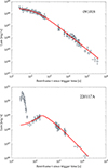 |
Fig. 1. Top: Example of an LC successfully modelled with Eq. (1). Bottom: Example of an LC, exhibiting a peak following steep decay, modelled with Eq. (4) as the afterglow rise caused by the deceleration of the relativistic ejecta. This example is one of the four out of nine GRBs whose rise was successfully modelled as RS emission. |
Unlike Liang09, we did not distinguish cases showing a well-defined plateau from those exhibiting an SPL. For the latter, we obtained unconstrained T0 values and calculated a 3σ upper limit. The reasoning behind our approach is that T0 is likely continuously distributed; therefore, modelling with Eq. (1) should be carried out on equal footing, encompassing the clear-cut plateau cases (for large values of T0) down to those showing a gentle steepening or no slope change (for relatively small values of T0).
As a result, 376 L-GRBs, 32 S-GRBs, and 16 SEE-GRBs passed the selection. Initially, there were ten L-GRBs, which did not pass because their LCs clearly show a re-brightening that follows steep decay. For these cases, we devised a different modelling approach, which is presented below.
In the prior activity model, this case may arise when the prompt gamma-ray emission ends before the deceleration of ejecta emitted at the zero time. Consequently, instead of adopting Eq. (1), we modelled the rise and subsequent decay as predicted for a homogeneous medium in two alternative cases, depending on the type of shock (reverse or forward) dominates. Each of these LCs was modelled as
![$$ \begin{aligned} L_x(t) = L_0\ \left[ \frac{1 - \alpha _1/\alpha _2}{\Big (\frac{t+T_0}{t_{\rm p}}\Big )^{n\alpha _1} + \Big (\frac{t+T_0}{t_{\rm p}}\Big )^{n\alpha _2} \Big (-\frac{\alpha _1}{\alpha _2}\Big )} \right]^{1/n}, \end{aligned} $$](/articles/aa/full_html/2025/11/aa56663-25/aa56663-25-eq4.gif)
where α1 < 0 and α2 > 0 are the rise and decay PL indices, tp the peak time, L0 the luminosity at peak, and the smoothness parameter n fixed to 5 (from Eq. (1) of Guidorzi et al. 2014). Instead of treating α1 and α2 as free parameters, we expressed them as a function of the PL index p, which describes the energy distribution of the shock-accelerated electrons that emit the afterglow synchrotron radiation. In particular, assuming that the slow cooling regime and the synchrotron frequency νm lie below X-rays, it is α1 = −3 and α2 = 3(p − 1)/4 for the FS case. Whereas for the RS, it is α1 = (3 − 6p)/2 and α2 = (3p + 1)/4 (Kobayashi 2000; Gao et al. 2013). Compared with Eq. (1), there are two additional parameters: tp, measured since the true zero time, and p, whereas α is no longer present. We assumed a uniform prior distribution for p in the range [2, 8], while tp shared the same prior of T0, with the constraint tp > T0 (otherwise, no afterglow peak would be visible in the data). Also for the cases modelled with Eq. (4), we rejected the solutions with p values < 10−3 for both the χ2 and runs tests. The bottom panel of Fig. 1 shows an example of successful modelling with RS. As a result, only one out of ten GRBs were discarded. Hereafter, the nine successful GRBs are referred to as the AG-rise sample.
3. Results
We restrict the following statistical analysis to the GRBs with well-constrained parameters. For a GRB to be considered, its uncertainties had to fulfil the following conditions: δ(log L0)≤0.3, δ(log T0)≤0.3, and δα ≤ 0.5. Similarly, for the AG-rise sample, we also imposed δ(log tp)≤0.3 and δp ≤ 0.2. Consequently, our sample shrank to 273 L-GRBs (nine of which belong to the AG-rise set), 19 S-GRBs, and eight SEE-GRBs, for a total of 300 GRBs with acceptable solutions and well-constrained parameters.
In agreement with the results obtained by Liang09 on a smaller sample, T0 is not correlated with the prompt gamma-ray emission duration, T90. We find no correlation between T0 and the intrinsic column density NH, z, which is the rest-frame hydrogen-equivalent column density in excess of the Galactic value for any given GRB direction. This column density is responsible for the photoelectric absorption of soft X-rays6.
Conversely, T0 is inversely proportional to L0, although with significant scatter. Calling y = log L0 and x = log T0, we modelled y = mx + q using the likelihood method of D’Agostini (2005), where the free parameters are m, q, and the intrinsic scatter σ. We modelled L-GRBs (excluding the nine AG-rise cases) separately from the S-GRBs and SEE-GRBs that were merged. Figure 2 shows the results, and Table 1 reports the best-fit parameters. For both groups, the PL index m is compatible with −1, that is the inverse proportionality between L0 and T0. They also share the same scatter of 0.75 dex. Only the normalisation is different, with the mean luminosity of L-GRBs being almost 10 times higher for a given T0. This relation shows that the difference between very luminous afterglows decaying with an SPL without any plateau, such as 061007 (Mundell et al. 2007), and canonical X-ray afterglows may be only apparent and simply reflect the different delays between the true start time of the catastrophic event and the observed prompt gamma-ray emission.
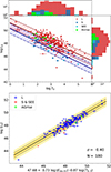 |
Fig. 2. Top: L0 vs. T0 for two separate groups: (i) L-GRBs (red circles, excluding the AG-rise cases), whose best-fit PL and 1σ uncertainty regions are shown by the solid red line and red-shaded area, respectively; (ii) S + SEE-GRBs (blue squares and cyan pentagons, respectively), whose best-fit PL is shown by the solid blue line within the blue-shaded area of the 1σ region. The L-GRBs of the AG-rise sample (green stars) were not used for the modelling. Also shown are the corresponding marginalised distributions. Bottom: L0-T0-Eγ, iso relation for the 180 GRBs with accurate measurements available, along with the best-fit model and 2σ uncertainty region. |
Best-fit parameters obtained with the D’Agostini (2005) method for the L0-T0 PL relation for the two separate groups: L-GRBs and S-GRBs merged with SEE-GRBs (top panel of Fig. 2).
We further explored the possible connection between the X-ray afterglow parameters extracted through the present analysis with other key observables that characterise the prompt gamma-ray emission: the isotropic-equivalent released energy Eγ, iso, the peak luminosity Lγ, iso (both referred to the 1–104 keV rest-frame band), and the intrinsic peak energy of the time-averaged ν Fν spectrum, Ep, i. We searched preferentially through GRB catalogues with a broad passband, which ensures reliable spectral modelling. In particular, values were taken from either the Konus-WIND catalogues (Tsvetkova et al. 2017, 2021) or elsewhere for some recent GRBs (e.g. Guidorzi et al. 2024). We ended up selecting 175 L-GRBs (three of which are AG-rise), three S-GRBs, and two SEE-SGRBs, for a total of 180 GRBs. We searched for possible correlations applying the principal component analysis (PCA)7. As a result, we found a three-parameter relation between L0, T0, and Eγ, iso which is common to all GRB classes considered in this work and whose scatter, 0.4 dex, is significantly smaller than that of the L0-T0 relation. Adopting the likelihood method from D’Agostini (2005), the best-fit relation is given by
with an intrinsic dispersion of σ = 0.404 ± 0.024, where Eγ, iso, 52 = Eγ, iso/(1052 erg) and T0, 3 = T0/103 (bottom panel of Fig. 2). A very similar result was obtained with Lγ, iso replacing Eγ, iso, with an intrinsic scatter, σ = 0.426 ± 0.025, that is slightly larger but compatible within errors. The analogous relation of Eq. (5) is
Finally, we found a four-parameter correlation with a slightly smaller scatter (σ = 0.373 ± 0.022 dex) by adding the PL index α as a fourth quantity to the relation in Eq. (5):
Apart from Eq. (7), the PL index α is not correlated with any individual quantity. Its mean, median, and standard deviation for the L-GRBs are 1.61, 1.44, and 0.62, respectively. The corresponding values for the S- and SEE-GRBs group are 2.2, 2.1, and 1.1, respectively; a Kolmogorov-Smirnov two-population test yields a p-value of 3 × 10⁻⁴ of a common parent distribution. The same comparison applied to the two sets of T0 cannot reject a common distribution (top panel of Fig. 2). The entire sample of T0 values is log-normally distributed with μ(log T0) = 3.0 and σ(log T0) = 0.8. Thus, while the distribution of the delay between zero time and prompt gamma-ray emission is similar for the two groups, on average, L-GRB X-ray afterglows decay slightly more shallowly than those of the S + SEE group.
4. Discussion and conclusions
The early X-ray emission covered by Swift/XRT, from as early as 60–100 s since the gamma-ray trigger, can be generally decomposed into two components: (1) internal dissipation, whose end is signalled by steep decay and can be interpreted as high-latitude emission (Lyutikov 2006; Zhang et al. 2006, 2009; Hascoët et al. 2012; Uhm & Zhang 2015; Lin et al. 2017; Ajello et al. 2019), along with the occasional presence of X-ray flares, whose internal origin is supported by a number of common properties with gamma-ray prompt pulses (Margutti et al. 2010; Guidorzi et al. 2015); (2) the X-ray afterglow, emitted by the interstellar medium swept up by an FS and possibly also by the relativistic ejecta as they are decelerated by a RS. In this work, we modelled the latter component within the context of the prior activity model, which assumes the zero time to precede the GRB itself by a time T0. Referring to the correct zero time, the afterglow LC is expected to exhibit a PL rise, followed by a PL decay, with no plateau whatsoever.
For 424 out of 463 GRBs with measured redshift, the X-ray afterglow behaviour is consistently modelled with either Eq. (1) or Eq. (4) as prescribed by this model, which consequently proved successful in approximately 90% of cases. The failure of the model in the remaining 10% is likely due to ongoing internal activity, which hampers the identification of the underlying afterglow, or in the so-called ‘internal plateau’ cases (both long and short), where the drop following the plateau is too steep to be accommodated as afterglow (Troja et al. 2007; Rowlinson et al. 2010).
The possibility that the prompt gamma-ray emission for most GRBs occurs some time (∼102–104 s in the GRB frame) after the beginning of the event appears to be plausible for a number of reasons. An immediate implication of this model is that similar behaviour should be observed in the X-ray and optical afterglow LCs. First of all, the distribution of the PL index α derived here is consistent with the typical values observed both in X-rays and in the optical (Zaninoni et al. 2013). For a sizeable fraction (approximately 40%; Panaitescu & Vestrand 2011) of early afterglows, optical and X-rays display different behaviours, especially within the first hundred seconds (Melandri et al. 2008; Oates et al. 2011). This can in most cases be ascribed to ongoing internal activity, which affects the X-ray emission and occasionally the optical emission as well (Kopač et al. 2013), along with possible changes in the optical PL decay caused by synchrotron break frequencies crossing the observed passband. Nonetheless, for 60–75% of cases, optical and X-ray show similar behaviours and LC morphologies, including the occurrence of plateaus (Oates et al. 2009; Panaitescu & Vestrand 2011; Roming et al. 2017). Moreover, the higher fraction of initially rising optical afterglows compared to the X-ray band is possibly due to ongoing internal activity, which may hide the simultaneous rise of the X-ray afterglow. In parallel, the numerous optical afterglows observed to decay early imply that ejecta deceleration and consequent afterglow peak must have occurred very early, potentially even before the GRB itself, as suggested by the prior activity model.
Our results show that the rest-frame delay, T0, between zero time and the gamma-ray trigger time, where the latter approximately corresponds to the start time of GRB itself, is continuously distributed, with values as low as a few tens of seconds or less (Fig. 2). Whenever T0 is a few seconds or less, the deviation from a straight PL becomes almost negligible using the trigger as zero time, and in this case no plateau is expected. A nice example of this case is offered by the luminous 061007: its broadband afterglow resembles an unbroken PL from ∼2 minutes from the GRB onset, continuing for several days with α ∼ 1.7 (Mundell et al. 2007). In our analysis, the X-ray LC shows evidence for a tiny but statistically significant deviation from a straight PL with log T0 = 0.43 ± 0.14, which is just a few seconds before the gamma-ray trigger time. So, in practice, the onset of its prompt gamma-ray emission essentially marks the beginning of the event, within a tolerance of a few seconds. The paucity of small delays in our sample is likely due to the fact that a high S/N is required to accurately measure a small curvature in the PL decay.
Another advantage of interpreting our results within the prior activity model is the common description of two apparently different behaviours: the plateau versus the rising X-ray afterglow (our AG-rise sample). The only difference between the two behaviours is that, for the former class, the afterglow peak must have occurred before the end of the GRB, whereas for the latter group the opposite is true, so that the steep decay flux drops quickly and deeply enough to let the rising afterglow emerge. To test our interpretation of the rising afterglows as resulting from the ejecta deceleration, we searched for simultaneous optical observations in the literature for the GRBs of our AG-rise sample. For the four out of nine events with available data, we find an optical peak consistent with ejecta deceleration, as also argued by various authors: 110213A (Wang et al. 2022), 140515A (Melandri et al. 2015), 181110A (Han et al. 2022), and 190829A (Dichiara et al. 2022; Salafia et al. 2022). The fact that the optical data for all the testable GRBs in our AG-rise sample confirm the ejecta deceleration scenario further corroborates our interpretation of the X-ray afterglow rise.
Thanks to the capability of identifying and localising X-ray transients over a large field of view, recent EP discovered X-ray emissions that lasted very long (∼103 s) and preceded (by up to several hundred seconds) the prompt gamma rays for a number of GRBs subsequently detected by some GRB experiments such as Fermi, SVOM, and Swift (Table 2). In addition to the discovery of so-called ‘ultra-long’ GRBs (Levan et al. 2014), these discoveries make the case for GRB engines that can operate much longer than previously thought, with soft emission that can start correspondingly earlier than the gamma rays. Although alternative interpretations of a GRB, such as a tidal disruption event, have been put forward, the recent case of the day-long EP250702a/GRB 250702B8 with the X-ray emission preceding the prompt gamma rays by one day, could be another compelling example (Levan et al. 2025).
Recent examples of GRBs, with X-ray emissions detected by EP long before the prompt gamma-ray emission.
The data in Table 2 were obtained by sifting through the General Coordinates Network (GCN) notices9 up to July 2025, selecting the common detections by both EP and gamma-ray instruments that routinely monitor the prompt gamma-ray emission. Table 2 reports two EP events that also triggered Swift and for which XRT recorded a prompt X-ray afterglow LC, which allowed us to test the prior activity model. In particular, the X-ray LC of EP241213a/GRB 241213A can be successfully modelled, yielding log T0 = 2.4 ± 0.1 (observer time), which corresponds to  s (top panel of Fig. 3). The EP/Wide-Field X-ray Telescope (WXT) detected X-ray emission 105 s before, which is not as early as our result but comparably close. In any case, an even earlier start than the EP/WXT time is possible in principle. The bottom panel of Fig. 3 shows the same LC with the zero time obtained here, which appears as an SPL. One concludes that the indication provided by the modelling of the early X-ray LC offers a hint about the true start of the phenomenon, which soft X-ray observations seem to support.
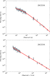 |
Fig. 3. Top: Observed XRT LC of 241213A in the observer frame, likewise detected by EP/WXT 105 s earlier (see Table 2). Successful modelling with a different zero time yields |

The case of EP250615a/GRB 250615A represents an interesting and complementary example: the XRT LC is a SPL from 100 s all the way to at least 104 s, with α = 1.610. This inevitably implies a small delay between X- and gamma rays and indeed the X-ray detection by EP/WXT differs by just a few seconds (Table 2), which is consistent with the 90% confidence upper limit of 13 s on T0 (observer frame) derived by us.
The case of the brightest GRB yet recorded, GRB 221009A, deserves a specific comment. At first glance, the XRT LC appears an SPL from 103 to 107 s (rest). However, following Williams et al. (2023), a broken PL provides a better description, with the PL index changing from 1.50 to 1.67 around a rest-frame break time of 7 × 10⁴ s, although the exceptional statistical quality of the data indicates a more complex behaviour. In our analysis, GRB 221009A was excluded from the selected sample due to very poor modelling, as evidenced by the p values of both χ2 and runs tests (7 × 10⁻³¹ and 6 × 10⁻¹⁶, respectively). The complexity of this behaviour, foregrounded by the unprecedented statistical quality of the dataset, might arise from the presence of residual internal activity. Observations in the TeV range by the Large High Altitude Air Shower Observatory (LHAASO) identified the afterglow reference time at T* = 226 s (observed) since the Fermi/Gamma-ray Burst Monitor (GBM) trigger time (Lesage et al. 2023), corresponding to rest-frame time of 196 s (LHAASO Collaboration 2023). This implies that the afterglow began right at the start of the peak of the kilo-electronvolt to mega-electronvolt activity within the observed 220 − 280 s window (Frederiks et al. 2023; Lesage et al. 2023). Adopting T* as the reference time, LHAASO Collaboration (2023) found evidence for a jet break at T* + 670 s, which corresponds to a rest-frame time of (T* + 670)/(1 + z) = 780 s since the prompt kilo-electronvolt to mega-electronvolt emission onset. The XRT LC begins after the putative jet break time, thus undermining the applicability of our analysis to this special GRB, as also evidenced by the poor modelling. Nonetheless, one cannot help but notice that GRB 221009A, as other extremely bright GRBs, shows no canonical behaviour in the early X-ray emission, as also noticed by O’Connor et al. (2023). Tera-electronvolt observations provide compelling evidence that the afterglow reference time occurs very close to the peak of the prompt gamma-ray emission. This automatically implies that no canonical X-ray plateau should be observed, as indeed is the case, in agreement with the basic prediction of the prior activity model.
There are several implications of the results: (a) the inferred gamma-ray efficiency decreases, since the energy released during the plateau phase is no longer attributed to internal dissipation (Ioka et al. 2006; b) the small fraction of long AG-rise cases (10/376) suggests that, in most cases, deceleration occurs before or at least by the end of the prompt gamma-ray emission. Within the thin-shell approximation, the deceleration time tp through a homogeneous medium with particle density n is
where Eiso, 52 = Eiso/1052 erg is the released kinetic energy and Γ0, 2 = Γ0/102 is the initial Lorentz factor (Sari & Piran 1999). Assuming typical values for L-GRBs, Eq. (8) yields tp values that are lower than most of our T0 estimates, thus explaining the small fraction of AG-rise cases. Another implication (c) concerns the jet break times, which would be increased by T0 compared to current estimates, thereby implying wider jet angles. Lastly, (d) GRB inner engines operate much longer and more frequently than that assumed so far. Figure 4 shows the ensemble of the 300 LCs with well-constrained parameters, referred both to the BAT trigger time (bottom) and to the estimated zero time (top). While the former case exhibits the flattening caused by most plateaus, the average behaviour in the latter case is an SPL with notable on-going internal activity (grey traits) superposed on the PL decay, extending up to 105 s.
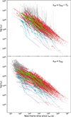 |
Fig. 4. Top: All the LCs displayed by shifting the rest-frame zero time backwards by T0. Red, blue, cyan, and green lines correspond to L-GRBs, S-GRBs, SEE-GRBs, and AG-rise cases, respectively. The grey portions were ignored by the modelling, being interpreted as internal activity. Bottom: Same data as in the top panel, except with the reference time coinciding with the BAT trigger time. |
Our analysis reveals a significant delay between the onset of the explosion and the prompt gamma-ray emission in short GRBs as well. The relativistic outflows appear to begin approximately 30 to 104 seconds before the gamma-ray trigger (see Fig. 2). These delays are substantially longer than the 1.7 second interval observed between the gravitational wave signal GW170817 and the short GRB 170817A (Abbott et al. 2017).
In the case of GRB 170817A, the observed off-axis jet means that the early X-ray afterglow does not reliably constrain the explosion time (T0). However, the gravitational wave signal provides a precise timestamp for the neutron star merger. It is unlikely that a powerful blast wave could be launched before the merger, although mechanisms such as resonant shattering of neutron star crusts may release energy of the order of ∼1047 erg, a few orders of magnitude lower than that of typical blast waves (Neill et al. 2022). Consequently, the explosion time offset for GRB 170817A is expected to be less than 1.7 seconds. As illustrated by the EP events (long-duration cases) listed in Table 2, the value of T0 may vary significantly from event to event. While extended emission in short bursts and recently observed long-duration merger events suggest that compact object mergers can power jets for durations exceeding 100 seconds, sustaining energy output for up to 104 seconds demands a revised understanding of the central engine.
Numerous past investigations have modelled the canonical X-ray afterglows through the end-of-plateau time, Ta, along with the X-ray luminosity at that time, La. An inverse proportionality between Ta and La was first discovered for 77 GRBs (Dainotti et al. 2010). Using 55 optimally selected GRBs, Xu & Huang (2012) subsequently found the three-parameter correlation,  , with an intrinsic scatter of 0.43 ± 0.05 dex. A similar result, with Lγ, iso replacing Eγ, iso, was later reported (Dainotti et al. 2016). More recently, the three-parameter correlation was confirmed over a sample of 174 GRBs and refined as
  with an intrinsic scatter of σ = 0.39 ± 0.03 dex. Remarkably, the same relation is found to hold true for all kinds of GRBs (Tang et al. 2019).
The fact that both the La − Ta inverse proportionality and the La − Eγ, iso − Ta correlation are very similar to our results (Table 1 and Eq. (5)) is not completely unexpected. By construction T0 is strongly correlated with Ta (at least for the cases for which a plateau can be confidently identified), as well as L0 with La. The two sets of parameters do not differ simply by definition, but especially in their meaning and implications, some of which were already discussed above. Moreover, our description takes a step further by including afterglow rising events, which are also modelled consistently within the prior activity model and yield results similar to those for other L-GRBs. Lastly, the different definitions of the two sets of parameters allow us to extend the three-parameter correlation over nine decades along L0, compared to six decades along La (see Fig. 8 of Tang et al. 2019).
The L0-T0 inverse proportionality can be interpreted within the prior activity model as follows: on average, the later the GRB prompt emission occurs relative to the zero time, the older the X-ray afterglow, which fades as a PL with an average index of −1. This is a typical value, especially from 102 to 104 s (Oates et al. 2011), and consistent with the prediction for an FS in the slow cooling regime. Conversely, interpreting the L0 − Eγ, iso − T0 correlation is less obvious. Taking L0 T0 as a rough proxy for the energy radiated by the early afterglow at the time of the prompt gamma-ray emission, this quantity should be linked to the energy released by gamma rays. A possible explanation is that the more energetic the initial ejecta responsible for the afterglow, the greater the energy dissipated into gamma rays, potentially constraining the way the inner engine releases its energy over time. The reason why short and long GRBs share the same relation is even less obvious, but its validity is an established property that should be considered.
Data availability
Tables 3–5 report the results and are available at the CDS via https://cdsarc.cds.unistra.fr/viz-bin/cat/J/A+A/703/A101
Acknowledgments
We thank the anonymous reviewer for their helpful comments. This work made use of data supplied by the UK Swift Science Data Centre at the University of Leicester. M.M. and R.M. acknowledge the University of Ferrara for the financial support of their PhD scholarships. M. B. acknowledges the Department of Physics and Earth Science of the University of Ferrara for the financial support through the FIRD 2024 grant.
References
- Abbott, B. P., Abbott, R., Abbott, T. D., et al. 2017, ApJ, 848, L13 [CrossRef] [Google Scholar]
- Ajello, M., Arimoto, M., Asano, K., et al. 2019, ApJ, 886, L33 [Google Scholar]
- Ascenzi, S., Oganesyan, G., Salafia, O. S., et al. 2020, A&A, 641, A61 [NASA ADS] [CrossRef] [EDP Sciences] [Google Scholar]
- Barthelmy, S. D., Barbier, L. M., Cummings, J. R., et al. 2005, Space Sci. Rev., 120, 143 [Google Scholar]
- Beniamini, P., Duque, R., Daigne, F., & Mochkovitch, R. 2020, MNRAS, 492, 2847 [NASA ADS] [CrossRef] [Google Scholar]
- Bissaldi, E., Meegan, C., & Fermi GBM Team. 2024, GCN, 37509, 1 [Google Scholar]
- Burns, E., & Svinkin, D. 2025, GCN, 41195, 1 [Google Scholar]
- Burrows, D. N., Hill, J. E., Nousek, J. A., et al. 2005, Space Sci. Rev., 120, 165 [Google Scholar]
- Chincarini, G., Moretti, A., Romano, P., et al. 2007, ApJ, 671, 1903 [NASA ADS] [CrossRef] [Google Scholar]
- Chincarini, G., Mao, J., Margutti, R., et al. 2010, MNRAS, 406, 2113 [NASA ADS] [CrossRef] [Google Scholar]
- D’Agostini, G. 2005, ArXiv e-prints [arXiv:physics/0511182] [Google Scholar]
- Dainotti, M. G., Willingale, R., Capozziello, S., Fabrizio Cardone, V., & Ostrowski, M. 2010, ApJ, 722, L215 [NASA ADS] [CrossRef] [Google Scholar]
- Dainotti, M. G., Postnikov, S., Hernandez, X., & Ostrowski, M. 2016, ApJ, 825, L20 [NASA ADS] [CrossRef] [Google Scholar]
- Dereli-Bégué, H., Pe’er, A., Ryde, F., et al. 2022, Nat. Commun., 13, 5611 [CrossRef] [Google Scholar]
- Dichiara, S., Troja, E., Lipunov, V., et al. 2022, MNRAS, 512, 2337 [Google Scholar]
- Dichiara, S., DeLaunay, J. J., Gupta, R., Sakamoto, T., & Neil Gehrels Swift Observatory Team. 2025, GCN, 40736, 1 [Google Scholar]
- Evans, P. A., Beardmore, A. P., Page, K. L., et al. 2009, MNRAS, 397, 1177 [Google Scholar]
- Falcone, A. D., Morris, D., Racusin, J., et al. 2007, ApJ, 671, 1921 [Google Scholar]
- Fan, Y., & Piran, T. 2006, MNRAS, 369, 197 [NASA ADS] [CrossRef] [Google Scholar]
- Foreman-Mackey, D., Hogg, D. W., Lang, D., & Goodman, J. 2013, PASP, 125, 306 [Google Scholar]
- Frederiks, D., Svinkin, D., Lysenko, A. L., et al. 2023, ApJ, 949, L7 [NASA ADS] [CrossRef] [Google Scholar]
- Gao, H., Lei, W.-H., Zou, Y.-C., Wu, X.-F., & Zhang, B. 2013, New Astron. Rev., 57, 141 [CrossRef] [Google Scholar]
- Gehrels, N., Chincarini, G., Giommi, P., et al. 2004, ApJ, 611, 1005 [Google Scholar]
- Genet, F., Daigne, F., & Mochkovitch, R. 2007, MNRAS, 381, 732 [NASA ADS] [CrossRef] [Google Scholar]
- Ghisellini, G., Ghirlanda, G., Nava, L., & Firmani, C. 2007, ApJ, 658, L75 [NASA ADS] [CrossRef] [Google Scholar]
- Granot, J., & Kumar, P. 2006, MNRAS, 366, L13 [NASA ADS] [Google Scholar]
- Guidorzi, C., Mundell, C. G., Harrison, R., et al. 2014, MNRAS, 438, 752 [NASA ADS] [CrossRef] [Google Scholar]
- Guidorzi, C., Dichiara, S., Frontera, F., et al. 2015, ApJ, 801, 57 [NASA ADS] [CrossRef] [Google Scholar]
- Guidorzi, C., Maccary, R., Tsvetkova, A., et al. 2024, A&A, 690, A261 [NASA ADS] [CrossRef] [EDP Sciences] [Google Scholar]
- Gupta, R., Gronwall, C., Page, K. L., Sakamoto, T., & Neil Gehrels Swift Observatory Team. 2024, GCN, 38547, 1 [Google Scholar]
- Han, S., Li, X., Jiang, L., et al. 2022, Universe, 8, 248 [Google Scholar]
- Hascoët, R., Daigne, F., & Mochkovitch, R. 2012, A&A, 542, L29 [NASA ADS] [CrossRef] [EDP Sciences] [Google Scholar]
- Hascoët, R., Daigne, F., & Mochkovitch, R. 2014, MNRAS, 442, 20 [Google Scholar]
- Ioka, K., Toma, K., Yamazaki, R., & Nakamura, T. 2006, A&A, 458, 7 [NASA ADS] [CrossRef] [EDP Sciences] [Google Scholar]
- Kobayashi, S. 2000, ApJ, 545, 807 [NASA ADS] [CrossRef] [Google Scholar]
- Kopač, D., Kobayashi, S., Gomboc, A., et al. 2013, ApJ, 772, 73 [CrossRef] [Google Scholar]
- Lesage, S., Veres, P., Briggs, M. S., et al. 2023, ApJ, 952, L42 [NASA ADS] [CrossRef] [Google Scholar]
- Levan, A. J., Tanvir, N. R., Starling, R. L. C., et al. 2014, ApJ, 781, 13 [Google Scholar]
- Levan, A. J., Martin-Carrillo, A., Laskar, T., et al. 2025, ApJ, 990, L28 [Google Scholar]
- LHAASO Collaboration (Cao, Z., et al.) 2023, Science, 380, 1390 [NASA ADS] [CrossRef] [Google Scholar]
- Li, D. Y., Xu, X. P., Wang, B. T., et al. 2024a, GCN, 37492, 1 [Google Scholar]
- Li, D. Y., Lian, T. Y., Wang, Y. L., et al. 2024b, GCN, 37909, 1 [Google Scholar]
- Liang, E.-W., Lü, H.-J., Hou, S.-J., Zhang, B.-B., & Zhang, B. 2009, ApJ, 707, 328 [NASA ADS] [CrossRef] [Google Scholar]
- Lin, D.-B., Mu, H.-J., Lu, R.-J., et al. 2017, ApJ, 840, 95 [Google Scholar]
- Liu, Y., Sun, H., Xu, D., et al. 2025, Nat. Astron., 9, 564 [Google Scholar]
- Lyutikov, M. 2006, MNRAS, 369, L5 [NASA ADS] [CrossRef] [Google Scholar]
- Margutti, R., Guidorzi, C., Chincarini, G., et al. 2010, MNRAS, 406, 2149 [NASA ADS] [CrossRef] [Google Scholar]
- Margutti, R., Zaninoni, E., Bernardini, M. G., et al. 2013, MNRAS, 428, 729 [NASA ADS] [CrossRef] [Google Scholar]
- Melandri, A., Mundell, C. G., Kobayashi, S., et al. 2008, ApJ, 686, 1209 [CrossRef] [Google Scholar]
- Melandri, A., Bernardini, M. G., D’Avanzo, P., et al. 2015, A&A, 581, A86 [NASA ADS] [CrossRef] [EDP Sciences] [Google Scholar]
- Mundell, C. G., Melandri, A., Guidorzi, C., et al. 2007, ApJ, 660, 489 [NASA ADS] [CrossRef] [Google Scholar]
- Neill, D., Tsang, D., van Eerten, H., Ryan, G., & Newton, W. G. 2022, MNRAS, 514, 5385 [NASA ADS] [CrossRef] [Google Scholar]
- Nousek, J. A., Kouveliotou, C., Grupe, D., et al. 2006, ApJ, 642, 389 [Google Scholar]
- Oates, S. R., Page, M. J., Schady, P., et al. 2009, MNRAS, 395, 490 [NASA ADS] [CrossRef] [Google Scholar]
- Oates, S. R., Page, M. J., Schady, P., et al. 2011, MNRAS, 412, 561 [Google Scholar]
- O’Connor, B., Troja, E., Ryan, G., et al. 2023, Sci. Adv., 9, eadi1405 [CrossRef] [Google Scholar]
- Oganesyan, G., Ascenzi, S., Branchesi, M., et al. 2020, ApJ, 893, 88 [NASA ADS] [CrossRef] [Google Scholar]
- Panaitescu, A., & Vestrand, W. T. 2011, MNRAS, 414, 3537 [Google Scholar]
- Planck Collaboration VI. 2020, A&A, 641, A6 [NASA ADS] [CrossRef] [EDP Sciences] [Google Scholar]
- Roming, P. W. A., Koch, T. S., Oates, S. R., et al. 2017, ApJS, 228, 13 [NASA ADS] [CrossRef] [Google Scholar]
- Rowlinson, A., O’Brien, P. T., Tanvir, N. R., et al. 2010, MNRAS, 409, 531 [NASA ADS] [CrossRef] [Google Scholar]
- Salafia, O. S., Ravasio, M. E., Yang, J., et al. 2022, ApJ, 931, L19 [NASA ADS] [CrossRef] [Google Scholar]
- Sari, R., & Piran, T. 1999, ApJ, 520, 641 [NASA ADS] [CrossRef] [Google Scholar]
- Shao, L., Dai, Z. G., & Mirabal, N. 2008, ApJ, 675, 507 [Google Scholar]
- Shen, R., & Matzner, C. D. 2012, ApJ, 744, 36 [NASA ADS] [CrossRef] [Google Scholar]
- Stratta, G., Dainotti, M. G., Dall’Osso, S., Hernandez, X., & De Cesare, G. 2018, ApJ, 869, 155 [NASA ADS] [CrossRef] [Google Scholar]
- SVOM/GRM Team, Wen-Jun tan, Dong, Y.-W., et al. 2024a, GCN, 37022, 1 [Google Scholar]
- SVOM/GRM Team, Zhang, Y.-Q., Wang, C.-W., et al. 2024b, GCN, 37921, 1 [Google Scholar]
- Tang, C.-H., Huang, Y.-F., Geng, J.-J., & Zhang, Z.-B. 2019, ApJS, 245, 1 [NASA ADS] [CrossRef] [Google Scholar]
- Toma, K., Ioka, K., Yamazaki, R., & Nakamura, T. 2006, ApJ, 640, L139 [NASA ADS] [CrossRef] [Google Scholar]
- Troja, E., Cusumano, G., O’Brien, P. T., et al. 2007, ApJ, 665, 599 [NASA ADS] [CrossRef] [Google Scholar]
- Tsvetkova, A., Frederiks, D., Golenetskii, S., et al. 2017, ApJ, 850, 161 [NASA ADS] [CrossRef] [Google Scholar]
- Tsvetkova, A., Frederiks, D., Svinkin, D., et al. 2021, ApJ, 908, 83 [NASA ADS] [CrossRef] [Google Scholar]
- Uhm, Z. L., & Beloborodov, A. M. 2007, ApJ, 665, L93 [NASA ADS] [CrossRef] [Google Scholar]
- Uhm, Z. L., & Zhang, B. 2015, ApJ, 808, 33 [NASA ADS] [CrossRef] [Google Scholar]
- Wang, X.-G., Chen, Y.-Z., Huang, X.-L., et al. 2022, ApJ, 939, 39 [NASA ADS] [CrossRef] [Google Scholar]
- Wang, Y. L., Li, A., Wang, W. X., Pan, H. W., & Einstein Probe Team. 2024, GCN, 37033, 1 [Google Scholar]
- Williams, M. A., Kennea, J. A., Dichiara, S., et al. 2023, ApJ, 946, L24 [NASA ADS] [CrossRef] [Google Scholar]
- Willingale, R., Starling, R. L. C., Beardmore, A. P., Tanvir, N. R., & O’Brien, P. T. 2013, MNRAS, 431, 394 [Google Scholar]
- Xu, M., & Huang, Y. F. 2012, A&A, 538, A134 [NASA ADS] [CrossRef] [EDP Sciences] [Google Scholar]
- Yamazaki, R. 2009, ApJ, 690, L118 [NASA ADS] [CrossRef] [Google Scholar]
- Yang, G. J., Liu, M. J., Zhao, Y. Q., et al. 2025, GCN, 40743, 1 [Google Scholar]
- Yuan, W., Zhang, C., Chen, Y., & Ling, Z. 2022, in Handbook of X-ray and Gamma-ray Astrophysics, eds. C. Bambi, & A. Sangangelo, 86 [Google Scholar]
- Zaninoni, E., Bernardini, M. G., Margutti, R., Oates, S., & Chincarini, G. 2013, A&A, 557, A12 [NASA ADS] [CrossRef] [EDP Sciences] [Google Scholar]
- Zhang, B., Fan, Y. Z., Dyks, J., et al. 2006, ApJ, 642, 354 [Google Scholar]
- Zhang, B.-B., Zhang, B., Liang, E.-W., & Wang, X.-Y. 2009, ApJ, 690, L10 [Google Scholar]
- Zhou, X. Y., Li, R. Z., Hu, D. F., et al. 2024, GCN, 38554, 1 [Google Scholar]
https://www.swift.ac.uk/xrt_live_cat/; when both window timing (WT) and photon counting (PC) mode average spectra were available, we used the weighted average photon index.
This was derived by modelling the late-time XRT spectrum available at the Leicester website with the XSPEC model cflux*TBabs*zTBabs*powerlaw, where the estimate for the Galactic NH from Willingale et al. (2013) was adopted.
GRB 250702B, D, and E are from the same source. However, to avoid confusion, we adhere to the GRB naming convention and refer to it as 250702B (Burns & Svinkin 2025).
All Tables
Best-fit parameters obtained with the D’Agostini (2005) method for the L0-T0 PL relation for the two separate groups: L-GRBs and S-GRBs merged with SEE-GRBs (top panel of Fig. 2).
Recent examples of GRBs, with X-ray emissions detected by EP long before the prompt gamma-ray emission.
All Figures
|
Fig. 1. Top: Example of an LC successfully modelled with Eq. (1). Bottom: Example of an LC, exhibiting a peak following steep decay, modelled with Eq. (4) as the afterglow rise caused by the deceleration of the relativistic ejecta. This example is one of the four out of nine GRBs whose rise was successfully modelled as RS emission. |
| In the text | |
|
Fig. 2. Top: L0 vs. T0 for two separate groups: (i) L-GRBs (red circles, excluding the AG-rise cases), whose best-fit PL and 1σ uncertainty regions are shown by the solid red line and red-shaded area, respectively; (ii) S + SEE-GRBs (blue squares and cyan pentagons, respectively), whose best-fit PL is shown by the solid blue line within the blue-shaded area of the 1σ region. The L-GRBs of the AG-rise sample (green stars) were not used for the modelling. Also shown are the corresponding marginalised distributions. Bottom: L0-T0-Eγ, iso relation for the 180 GRBs with accurate measurements available, along with the best-fit model and 2σ uncertainty region. |
| In the text | |
|
Fig. 3. Top: Observed XRT LC of 241213A in the observer frame, likewise detected by EP/WXT 105 s earlier (see Table 2). Successful modelling with a different zero time yields |
| In the text | |
|
Fig. 4. Top: All the LCs displayed by shifting the rest-frame zero time backwards by T0. Red, blue, cyan, and green lines correspond to L-GRBs, S-GRBs, SEE-GRBs, and AG-rise cases, respectively. The grey portions were ignored by the modelling, being interpreted as internal activity. Bottom: Same data as in the top panel, except with the reference time coinciding with the BAT trigger time. |
| In the text | |
Current usage metrics show cumulative count of Article Views (full-text article views including HTML views, PDF and ePub downloads, according to the available data) and Abstracts Views on Vision4Press platform.
Data correspond to usage on the plateform after 2015. The current usage metrics is available 48-96 hours after online publication and is updated daily on week days.
Initial download of the metrics may take a while.