| Issue |
A&A
Volume 704, December 2025
|
|
|---|---|---|
| Article Number | A331 | |
| Number of page(s) | 22 | |
| Section | Numerical methods and codes | |
| DOI | https://doi.org/10.1051/0004-6361/202452223 | |
| Published online | 24 December 2025 | |
Introducing the Rhea simulations of Milky Way-like galaxies
I. Effect of gravitational potential on morphology and star formation
1
Universität Heidelberg, Zentrum für Astronomie, Institut für Theoretische Astrophysik,
Albert-Ueberle-Str. 2,
69120
Heidelberg,
Germany
2
Centre de Recherche Astrophysique de Lyon UMR5574, ENS de Lyon, Univ. Lyon1, CNRS, Université de Lyon,
69007
Lyon,
France
3
École Polytechnique Fédérale de Lausanne, Observatoire de Sauverny,
Chemin Pegasi 51,
1290
Versoix,
Switzerland
4
Universität Heidelberg, Interdisziplinäres Zentrum für Wissenschaftliches Rechnen,
Im Neuenheimer Feld 225,
69120
Heidelberg,
Germany
5
Harvard-Smithsonian Center for Astrophysics,
60 Garden Street,
Cambridge,
MA
02138,
USA
6
Elizabeth S. and Richard M. Cashin Fellow at the Radcliffe Institute for Advanced Studies at Harvard University,
10 Garden Street,
Cambridge,
MA
02138,
USA
7
Université Paris-Saclay, Université Paris Cité, CEA, CNRS, AIM,
91191
Gif-sur-Yvette,
France
8
Istituto di Astrofisica e Planetologia Spaziali (IAPS), INAF,
Via Fosso del Cavaliere 100,
00133
Roma,
Italy
9
SUPA, School of Physics and Astronomy, University of St Andrews,
North Haugh,
St Andrews
KY16 9SS,
UK
10
Como Lake centre for Astrophysics (CLAP), DiSAT, Universitá degli Studi dell’Insubria, Dipartimento di Scienza e Alta Tecnologia,
Via Valleggio 11,
22100
Como,
Italy
11
Alma Mater Studiorum Università di Bologna, Dipartimento di Fisica e Astronomia (DIFA),
Via Gobetti 93/2,
40129
Bologna,
Italy
12
INAF – Osservatorio Astrofisico di Arcetri,
Largo E. Fermi 5,
50125
Firenze,
Italy
★ Corresponding authors: This email address is being protected from spambots. You need JavaScript enabled to view it.
; This email address is being protected from spambots. You need JavaScript enabled to view it.
; This email address is being protected from spambots. You need JavaScript enabled to view it.
Received:
12
September
2024
Accepted:
24
August
2025
Abstract
The Milky Way is a complex ecosystem. We can obtain detailed observations of it by probing the physical mechanisms that determine its interstellar medium. For a detailed comparison with observations and to provide theories for missing observables, the Milky Way must be modelled as accurately as possible. However, details of the Galactic structure are not fully defined by observations, which raises the need for more generalised models. With the Rhea simulations, we present a set of Milky Way-like simulations containing detailed physics of the interstellar medium as well as star formation and stellar feedback. We conducted two simulations that differ in the gravitational potential: one fitted to several structural details derived from observations and another that only reproduces the most basic quantities. We find little difference in the overall morphology except for the bar region, which funnels gas towards the Galactic inner region and therefore prevents quenching in the centre. Despite differences with galacto-centric radius, the global star formation rate is almost identical in both setups. A spiral arm potential does not influence properties of groups of formed stars. A bar potential, however, reduces the size and formation time of those associations. We conclude that a spiral arm potential has little influence on star formation in the Galaxy, except for producing long-lived spiral structures instead of transient ones, and that a galactic bar potential has a noticeable influence on star formation, mainly within the innermost 2.5 kpc.
Key words: methods: numerical / galaxy: evolution / galaxy: structure
© The Authors 2025
 Open Access article, published by EDP Sciences, under the terms of the Creative Commons Attribution License (https://creativecommons.org/licenses/by/4.0), which permits unrestricted use, distribution, and reproduction in any medium, provided the original work is properly cited.
This article is published in open access under the Subscribe to Open model. This email address is being protected from spambots. You need JavaScript enabled to view it. to support open access publication.
1 Introduction
The Milky Way, as a typical spiral galaxy of the type that dominates the star formation in our present-day Universe (Kennicutt & Evans 2012; Bland-Hawthorn & Gerhard 2016), is a unique laboratory for investigating the physical processes of galaxy evolution. It provides the opportunity for direct observation of processes such as the formation of molecular clouds, stars, and stellar feedback. In no other galaxy can these processes be studied in as much detail.
However, the galactic context of star formation and the corresponding stellar feedback is still poorly understood, even within the Milky Way, and the influence of the galactic potential and galactic dynamics on local star formation is an open debate. Star formation is known to be a very inefficient process (for a review, see e.g. Girichidis et al. 2020). A key question is whether this inefficiency is entirely due to the influence of stellar feedback, magnetic fields, and gas turbulence, as discussed in Girichidis et al. 2020, or whether galactic dynamics and the galactic potential also play an important role in regulating star formation efficiency (SFE).
The central molecular zone (CMZ) in the centre of the Milky Way is a compact region of about 3–7×10⁷ M⊙ (Molinari et al. 2011; Tokuyama et al. 2019) of cold, dense clouds that are fueled by the dust lanes caused by the Galactic bar potential. The SFR of the CMZ, however, is observed to be just 0.06–0.14 M⊙ yr−1 (Yusef-Zadeh et al. 2009; Immer et al. 2012; Longmore et al. 2013), which is more than a factor of ten smaller than what would be predicted from its gas mass and density (Longmore et al. 2013; Kruijssen et al. 2014). Simulations (e.g. Seo & Kim 2013; Seo et al. 2019; Sormani et al. 2020; Moon et al. 2021) suggest that this is because the star formation rate (SFR) is more closely correlated to the gas inflow rate than to the mass of the region (even though Seo & Kim (2013) find it unlikely for the bar potential alone to be responsible for the suppression of the SFR). The galactic potential therefore seems to play a crucial role in the regulation of star formation in this region, as the bar potential controls the gas inflow rate. Also, the presence of a bar itself has been shown to alter the SFR of a galaxy (e.g. Vera et al. 2016; Scaloni et al. 2024).
Another example are spiral arms, whose role in star formation is still heavily debated. It is unclear if they mainly serve as triggers of star formation by increasing the density of incoming gas and the SFE or if they simply organise star-forming gas with no impact on the star formation process itself. As an example, Foyle et al. (2010) found very similar SFEs in arm and interarm regions of NGC 5194 and NGC 628, whereas Seigar & James (2002) found significant enhancement of SFR in the vicinity of spiral arms, arguing for triggered star formation. Numerical simulations tend to find no triggering of star formation in spiral arms. However, Dobbs et al. (2011) find that a spiral potential can increase the SFR indirectly by enabling the formation of long-lived and strongly bound clouds. Kim et al. (2020) find that the global SFR is only moderately enhanced by a spiral arm potential, but that the star formation is reorganised such that the majority of star formation happens in the spiral arms. The question is even harder to answer without the knowledge of whether the spiral structures are long-lived (as suggested by the density wave theory, Lin & Shu 1964; Shu 2016) or whether they are transient features (as suggested by the self-propagating star formation model, Mueller & Arnett 1976; Gerola & Seiden 1978).
Such reorganisations of star formation throughout the galactic disc can have substantial consequences for the appearance of a galaxy. Star formation itself shapes the surrounding gas. However, subsequent stellar feedback such as stellar winds and supernovae affect the galactic disc up to several hundreds of parsecs. Clustered star formation, which results in subsequent clustered winds and supernovae, can form superbubbles that tear enormous holes in the gaseous structure of the galaxy (see e.g. Ferrière 2001). Strong star formation activity might even be the reason for the formation of the Fermi bubbles (Su et al. 2010; Dobler et al. 2010) in the Galactic centre (Crocker & Aharonian 2011; Crocker 2012). Local variations of the SFR are therefore of utter importance for the general appearance of a galaxy and are a driver for galactic evolution.
For the Milky Way itself, it is hard to estimate the true Galactic potential and the star formation properties anywhere outside the greater solar neighbourhood because of our particular observational placement in it. Nevertheless, the Galaxy has been sampled across a wide range of wavelengths, revealing many facets of its complex system (e.g. Hi-GAL, Molinari et al. 2010; SEDIGISM, Schuller et al. 2017; CHIMPS, Rigby et al. 2016; FQS, Benedettini et al. 2020; THOR, Beuther et al. 2016; and eROSITA, Predehl et al. 2021; for stars see Gaia Collaboration (2023) or Benjamin et al. 2005; Carey et al. 2009 for infrared surveys; and for nearby star-forming regions, see e.g. Brunthaler et al. (2021)). However, basic Galactic properties are still under debate, such as how many spiral arms are present (Hou & Han 2014; Drimmel 2000; Reid et al. 2019) and the exact structure and relative position of the Galactic bar (see e.g. Nishiyama et al. 2005; Cabrera-Lavers et al. 2008; Vanhollebeke et al. 2009; Majaess 2010). One therefore might wish for a more general approach in terms of potential and structure when modelling a Milky Way-like galaxy.
There are numerous simulations aimed at explaining and supplementing observations. Many studies have examined the formation of the Milky Way in a cosmological context (Elias et al. 2018; Pillepich et al. 2021; Ortega-Martinez et al. 2022; Gensior et al. 2023; Li et al. 2021; Grand et al. 2017; Agertz et al. 2021; Fattahi et al. 2016; Buck et al. 2020; Wetzel et al. 2016), but these studies typically have too coarse of a resolution to properly represent the small-scale physics of the interstellar medium (ISM; e.g. the formation of molecular clouds).
A much higher resolution can be reached in simulations of the Milky Way as an isolated galaxy. This approach was used, for example, by Pettitt et al. (2014), who used the SPH code PHANTOM to simulate a Milky Way-like galaxy with a modular potential of bulge, halos, disc, and spiral arms in a 13 kpc disc. With the AMR code RAMSES, Renaud et al. (2013) simulated a 28 kpc gaseous disc of a Milky Way analogue with star formation and stellar feedback for a few cloud lifetimes. They adopted a dynamic potential including the dark matter (DM) halo, the spheroid and bulge, and the thin and thick discs. Non-axisymmetric features such as the bar and spiral arms were formed during the run from instabilities in the velocity profiles. The simulations of Jeffreson et al. (2020) used the moving-mesh code AREPO to study giant molecular clouds in the disc of a Milky Way-like galaxy. They tested the impact of several potentials (consisting of different compositions of the stellar bulge, stellar disc, and DM halo) on a gaseous disc with an exponential density profile (scale radius 7.4–7.7 kpc). However, they ignored the Galactic bar in their potential. Wibking & Krumholz (2023) simulated a Milky Way-like galaxy with GIZMO to study the Galactic magnetic field. However, their simulation as well lacks a galactic bar. The same applies for Konstantinou et al. (2024), who studied the B − ρ relation in a Milky Way-like galaxy. They included a DM halo, a thin stellar disc (truncated at 12 kpc), a gaseous disc (truncated at 15 kpc), and a gaseous halo.
However, a simulation of the whole Milky Way galaxy that allows for a study of the influence of the Galactic potential on star formation is still missing, as either essential parts of the potential are not included or the simulation time is too short to produce meaningful statistics. The Rhea simulation suite is targeted to fill this gap. Here, we present its first set of simulations. Our simulations include an elaborate external Milky Way potential (with non-axisymmetric features of a bar and spiral arms) that allows for a close match to observations of dynamical properties as well as star formation and supernova feedback. To investigate the influence of the potential, we modelled the same set of initial conditions also with a potential that only reproduces the most basic features of the velocity curve. This paper, which introduces the main setup and discusses the numerical techniques, is the first in a series targeting different features and results of the simulations. Here, we focus on hydrodynamical simulations, whereas follow-up studies will include magnetic fields and cosmic rays. As a first application, we studied the influence of the potential on the properties of star formation, as well as its general morphology.
The paper is organised into the following sections: in Section 2, we begin with the general simulation methods and set up, the adopted star formation and stellar feedback routines, the different potentials, and further simulation details. We describe the morphological and structural properties in Section 3. In Section 4, we analyse the differences in star formation arising between the two studied potentials. We briefly discuss the caveats of our study in Section 5.1 and in Section 5.3 we summarise our findings.
Specifications of the simulations presented in this work.
2 Methods
We modelled an isolated Milky Way-like galaxy with a fixed external potential. In the following, we present our numerical setup as well as the parameters that we used.
2.1 Numerical framework
In this work, we present a set of two simulations of a Milky Way-like galaxy (+2 simulations for a resolution study, specified in Table 1). We used the moving-mesh code AREPO (Springel 2010; Weinberger et al. 2020), which solves the equations of hydrodynamics while also accounting for the gravitational accelerations produced by the gas and by collisionless components such as stars and dark matter. The fundamental equations of hydrodynamics in a non-cosmological environment (a = 1) can be written as (Weinberger et al. 2020; Pakmor & Springel 2013)
 (1)
(1)
 (2)
(2)
 (3)
(3)
with the total energy (per unit volume) and pressure being
 (4)
(4)
 (5)
(5)
Here, ρ is the mass density, u is the flow velocity vector, H and Λ are respectively the radiative heating and cooling terms, and eth is the thermal energy per unit mass. The gravitational potential, Φ, is the sum of the external potential, Φext, described below; the gas self-gravity, Φgas; and the potential due to the star particles, Φstars. We set the adiabatic index to γ = 5/3 for all gas, even if it is molecular. This is justified because the vast majority of the molecular gas in our simulations has a temperature of T < 200 K, which is too low to excite the internal degrees of freedom of the H2 molecule.
The hydrodynamical equations are solved on a 3D time dependent Voronoi mesh. The mesh generating points defining the Voronoi tessellation move at the local fluid velocity, such that the grid can follow the fluid. The cell mass is held approximately constant, and therefore the cell volume continuously adapts to regions of differing density, making AREPO a quasi-Lagrangian scheme.
2.2 Resolution
In its standard setting, AREPO uses a mass resolution, not a volume resolution, for the gas cells. Cells with masses that surpass a user-set target mass by more than a factor of two get split into smaller cells, while those that have a mass lower than the target mass by a factor of 0.5 get removed. We ran our simulations with a fiducial target mass of 3000 M⊙, but also perform two comparison runs with a lower target mass of 1000 M⊙ (see Table 1).
In addition, we also limited the maximum and minimum volumes that our cells are allowed to have, refining or de-refining as appropriate to enforce these limits. Within the whole box, the minimum cell volume was set to 1 pc3 and the maximum to 2 kpc3. It is refined if a cell exceeds this volume by a factor of two. Moreover, in the area of the Galactic disc, i.e. in a cylinder with 30 kpc in radius and 2 kpc in thickness, located at the centre of the box, we set an upper volume limit of 106 pc3. This ensures a sufficient volume resolution within the Galactic disc. In Fig. B.1, we show the density-volume distribution of gas cells at about 2500 Myr for F3000HD, as a representative example. The mass refinement and the total box volume refinement are strictly adhered to; however, one can see some disc cells that are larger than allowed by their refinement criterion. We explain this by cells existing near the boundary of refinement, moving into the refinement region. Those cells may need multiple refinement cycles to meet the refinement criterion, depending on their size, as during each refinement cycle they can only refine once.
The gravity solver of AREPO treats each gas cell as a point mass with an adaptive softening length, chosen from tabulated softening lengths depending on the cell size. In our simulations, the tabulation starts at 0.01 pc and has a logarithmic spacing with a multiplicative factor of 1.15. The softening length is then chosen as the closest value from this tabulation to 2 × rcell, where rcell is the radius of a sphere equivalent in volume to the gas cell. Star particles are also treated as point masses, with a fixed softening length of 6.47 pc.
2.3 Initial conditions
We started our simulations with a smooth gaseous disc with a density distribution given by
 (6)
(6)
in cylindrical coordinates (Sormani et al. 2019), with zd = 85 pc, Rd = 7 kpc, Rm = 1.5 kpc and Σ0 = 50 M⊙ pc−2. The total mass of the gas disc is ∼1010 M⊙. We truncate this distribution at a radius of 30 kpc, as expected from the maximum radial extent of HI in the Milky Way (see, for example, Kalberla & Dedes 2008; McClure-Griffiths et al. 2023). Further out, the density is set to a minimum density ρmin = 10−31 g cm−3 . We do not impose a cut in the z-direction, but set a minimum density of 10−31 g cm−3 here as well. The gas is set to solar metallicity and a gas-to-dust ratio similar to the local ISM. We use an initial abundance (A (X) = log (X/H) + 12) of 8.15 for carbon and 8.5 for oxygen (Sembach et al. 2000). The disc is embedded in a box of 150 kpc side length with periodic boundary conditions. The large box size prevents outflows from reaching the box boundaries, and thus it also stops boundary effects from happening. The gas initially has a temperature of 1.3×10⁴ K throughout the whole box. After generating the simulation box with this density distribution, we impose the velocity corresponding to the used potential on the gas, while accounting for the pressure gradient.
2.4 Simulation phases
Without turbulence, our initial disc with its smooth density distribution would collapse immediately, forming a huge number of stars, which, with their feedback, would destroy the Galactic disc. To prevent that, we initially set a temperature floor of 100 K to prevent the gas from cooling too much and induce turbulence in an initial phase I via modulated supernova feedback.
The procedure is as follows: we start the simulation with star formation enabled, but set the lifetime of stars to a tenth of their normal value. We show the gaseous disc on initial conditions in Fig. A.1, left column. Additionally, we enable mass return with the supernova, i.e. the supernova do not just return energy or momentum to the surrounding gas, but with each exploding supernova, the mass of the star particle MstarP is reduced by MstarP/NSN,tot, where NSN,tot is the total number of supernovae going off in the star particle, i.e. the number of stars with a mass >8 M⊙ at the formation time of the star particle. The mass each supernova returns is distributed evenly to the cells within the injection radius.
In this phase, the stars in the star particles explode as supernovae relatively rapidly after their formation, and the mass return ensures that the star particles are gone when all stars are exploded, i.e. that no mass is locked up in the star particles. The energy and momentum injection by the supernova induce turbulence in the disc.
Over the course of 1 Gyr we increase the lifetime of the stars in newly formed star particles back to their normal, tabulated lifetime. After reaching the normal lifetime, we run phase I for another Gyr, resulting in a total time in phase I of 2 Gyr. We show the result of this phase I in the Appendix, Fig. A.1.
After this initial phase I, we continue with phase II with regular stellar lifetimes and without mass return during supernova events. In this paper, we only analyse phase II.
2.5 Chemistry and thermodynamics
We use a chemical network to model the non-equilibrium chemical composition of the gas. At our fiducial resolution (see Section 2.2 below), we do not expect to be able to accurately model the atomic-to-molecular transition (see e.g. Seifried et al. 2017 or Joshi et al. 2019 for a discussion of the required resolution) and hence any results regarding the H2 or CO content of the gas must be treated with great caution. Our decision to follow the chemical evolution of the gas despite this fact is motivated by two main considerations. First, and most importantly, modelling the chemistry allows us to track the fractional ionisation of the gas. This plays an important role in determining the efficiency of both photoelectric heating and C+ cooling (Wolfire et al. 1995), and tracking its value on the fly in the simulation therefore allowed us to model the thermal evolution of the gas much more accurately than if we were using a simple tabulated cooling function. Second, we plan to perform a follow-up on our current calculations in a future work in which we will perform much higher resolution ‘zoom-ins’ of selected regions such as supernova bubbles or the emerging eRosita bubble analogues. Having chemical information already available in the output from our current simulations will therefore greatly facilitate their use as initial conditions for these upcoming calculations.
In our simulations, we use the NL97 chemical network of Glover & Clark (2012). This combines the hydrogen chemistry network from Glover & Mac Low (2007a,b) and a highly simplified CO chemistry network introduced by Nelson & Langer (1997). To model the H2 and CO self-shielding and the dust shielding from the UV interstellar radiation field, we use the TREECOL algorithm developed by Clark et al. (2012). We consider a spatially and temporally constant background radiation field, using solar neighbourhood values for the strength and spectral shape from Draine (1978) in the UV and Mathis et al. (1983) in the optical and infrared. We also take into account cosmic ray ionisation, with a rate ζH = 3 × 10⁻¹⁷ s−1 for atomic H, and suitably scaled values for other chemical species.
Apart from adiabatic expansion and contraction, which are treated in the standard hydrodynamics of AREPO (Springel 2010), we take into account several additional radiative and chemical heating and cooling processes (Clark et al. 2019). The main heating processes include the photoelectric effect, H2 pho-todissociation, chemical heating due to UV pumping of H2 and H2 formation on dust grains, and heating associated with cosmic ray ionisation. The main cooling processes include fine structure line emission from C+ and O, rovibrational line emission from H2 and CO, collisional ionisation of atomic H and dissociation of hydrogen, gas-grain energy transfer, ion recombination on grain surfaces, and Compton cooling. A full list of all included processes is given in Glover et al. (2010), with later additions and modifications described in Glover & Clark (2012) and Mackey et al. (2019).
Throughout the simulation, we impose a temperature floor. During phase I (see Sect. 2.4), we set this temperature floor to 100 K, to prevent the gas from cooling and forming a large number of star particles in the same simulation region. In phase II, we drop it to 20 K. This is lower than the characteristic temperature of the gas at the highest densities reached in our simulations (see Fig. 3), and so we do not expect this temperature floor to significantly affect the dynamical behaviour of the gas.
2.6 Star formation
To represent clusters of stars, we use star particles, i.e. point-like structures in the code, that form out of gas and thereafter interact only via gravitational forces. At the resolution used in our simulations, each star particle has a mass much greater than a typical star and, therefore, represents multiple stars. With the information about the star particle, we also store a list of the masses and lifetimes of the massive (M > 8 M⊙) stars that each particle represents (see Section 2.7). This is used to determine the stellar feedback produced by each star particle, as explained in Section 2.7. In contrast to the sink particles used in some simulations of galactic-scale star formation (e.g. Tress et al. 2020a), which represent a mix of dense gas and stars, the star particles used here represent only stars, i.e. the full mass of a gas cell gets converted into stellar mass, no hidden gas remains in the star particle.
To decide whether gas within an active grid cell forms a star particle during a given time step, we investigated the gas in terms of its Jeans instability. This approach differs from a density-threshold approach (adopted in e.g. Renaud et al. 2013; Jeffreson et al. 2020) and therefore prevents artificial star formation in hot compressed gas as it might occur in feedback regions. We first calculated the Jeans mass, MJ, of the cell via
 (7)
(7)
 (8)
(8)
 (9)
(9)
where eth is the specific internal energy of the cell and G is the gravitational constant. If the cell’s mass exceeds 12.5% of its local Jeans mass, we flag the cell as possibly star forming. This number is chosen such that star formation starts when the Jeans mass is resolved by less than eight cells. If the mass exceeds the Jeans mass, we immediately force it to form a star particle. By doing so, we prevent dense gas from accumulating on the grid and forcing small time steps. This procedure was first introduced in Smith et al. (2021).
If the cell was flagged as possibly star forming, we calculated its freefall time, tff, and SFR:
 (10)
(10)
 (11)
(11)
where Mcell is the mass of gas in the cell. We set the SFE per freefall time, ϵ, to a value of 1%, which was motivated by recent observational determinations (see e.g. Sun et al. 2023). However, we varied this parameter between 0.1% and 10% and found it to have no strong influence on the overall SFR in the simulation, owing to efficient self-regulation of star formation.
Given the SFR of the cell, we then determined its probability, p, of forming a star during the current time step using the same expression as in Springel & Hernquist (2003):
 (12)
(12)
 (13)
(13)
where ∆t is the time step of the cell. MstarP is the desired mass of the star particle, which equals Mcell in most cases. That means that usually a full gas cell is converted into a star particle. However, if the mass of the cell exceeds the target mass (see Sect. 2.2) by more than a factor of 2, i.e. if the cell would have been split into two in the next time step, only half of the cell’s mass gets converted into a star particle, and the other half remains as gas.
The time step of star-forming cells is limited to
 (14)
(14)
With that,  , and therefore the probability for a star particle to form cannot exceed one until the target mass chosen for the star particle is ten times smaller than the mass of the gas cell. Since we set the target mass for the star particles to equal the target mass for the gas cells, and the code prevents gas cells from exceeding their target mass by more than a factor of 2, that does not happen.
After the star formation probability was calculated, we drew a random number, xSF, from a uniform distribution between 0 and 1, and in case xSF < p, the full gas cell converts into a star particle, i.e. all the gas in the cell is converted into stars. Otherwise, it remains as gas.
2.7 Stellar feedback
In these simulations, we used the supernova feedback routine described in Tress et al. (2020a), with some adjustments towards the used star particles. In the first step, the star particles are populated with individual stars by sampling from the initial mass function (IMF) following the algorithm described in Sormani et al. (2017). For the IMF-sampling we use the high-mass end of the Kroupa IMF (Kroupa 2001), the whole mass of the star particle is in stars with no locked-up gas. Stars with a mass between 8 M⊙ and 120 M⊙ assigned, which are thought to explode as supernovae, get a lifetime in accordance with Table 25.6 in Maeder (2008); we linearly interpolate between the different mass bins in the table. After this lifetime the star explodes as a supernova at the location of its star particle.
The supernovae explode in one of two modes: energy or momentum injection. The decisive factor here is the radius of the supernova remnant at the end of the Sedov-Taylor phase. At solar metallicity, this is (Blondin et al. 1998; Tress et al. 2020a)
 (15)
(15)
where  is the local mean number density. If RST > Rinject, an energy of 1051 erg is injected isotropically in the injection region (cells within Rinject) as thermal energy and the contained gas is fully ionized. Otherwise the terminal momentum (derived e.g. in Gatto et al. 2015; Kim & Ostriker 2015; Martizzi et al. 2015),
 (16)
(16)
is injected directly into the cells within the injection region. In this case, the temperature or ionisation state of the gas is not changed. We use an injection radius of Rinject = 100 pc. This radius ensures a sufficient number of cells within the injection radius.
For supernovae in very low density environments, RST is large, and consequently, the injected thermal energy can lead to unphysically high temperatures. In such cases, we limited the energy injection as follows: if the temperature of a supernova-heated cell, Tcurrent = eth(γ − 1)µmp/kB, is larger than 107 K, we did not inject any more energy. If the estimated temperature after energy injection,
 (17)
(17)
is larger than the threshold value, we reduced the injected energy, einjected, by a factor of
 (18)
(18)
2.8 Gravitational potentials
For our setups, the gravitational potential is the sum of an external potential, Φext, and the contribution due to self-gravity of the gas and stars, Φsg:
 (19)
(19)
where the latter is found by solving the Poisson equation
 (20)
(20)
using the standard gravitational tree in AREPO (Weinberger et al. 2020). We used parameterised external potentials for the components that we do not include such as dark matter and the low-mass stars as well as old populations of stars because this allows for a better tuning towards Milky Way features. This is different from a live potential, as used by Durán-Camacho et al. (2024), for example. We compared two different setups concerning the external potentials: a logarithmic potential, resulting in a flat velocity curve (Binney & Tremaine 2008), and a realistic potential fine-tuned to match the known properties of the distribution of dark matter, gas, and stars in the Milky Way (Hunter et al. 2024). We refer to the potentials as the ‘flat potential’ and the ‘Milky Way potential’ from here onwards.
2.8.1 Flat external potential
The flat external potential is a logarithmic potential from Binney & Tremaine (2008) (Eq. (2.71a)) and is written as
 (21)
(21)
where Rc = 100 pc and v0 = 220 km/s are constants and qΦ = 0.8 is the axis ratio of the equipotential surfaces. This results in a circular velocity at the Galactocentric radius, Rgal, in the equatorial plane (Eq. (2.71b) of Binney & Tremaine 2008) of
 (22)
(22)
2.8.2 Milky Way external potential
The Milky Way external potential of Hunter et al. (2024) was generated from analytic density profiles including the central black hole (SgrA*), the nuclear stellar cluster, the nuclear stellar disc, the Galactic bar, axisymmetric and non-axisymmetric (spirals) disc components, and the DM halo using the AGAMA code (Vasiliev 2019). The chosen model enforces four spiral arms with a pattern speed of Ωspa = −22.5 km s−1 kpc−1 and a galactic bar with a pattern speed of Ωbar = −37.5 km s−1 kpc−1 and is fully described in Hunter et al. (2024). Figure 1 depicts the non-axisymmetric components of the external potential, the spiral arm (left) and the bar (right) at 2500 Myr. We introduced these non-axisymmetric components linearly within the first 150 Myr of the simulation to avoid transients. The model presented in Hunter et al. (2024) includes the influence of the gas disc. However, in our simulations, we excluded this component of the potential and replaced it with the self-consistently computed one of the gaseous disc in our simulation box.
3 Morphology
A galaxy is a non-linear and highly complex system with many processes at play. The gravitational potential of old stars and DM, which we refer to as the external potential, is one of them. In this section, we study the details of the used gravitational potentials and their influence on the morphology of the gas and the newly created stars. We are interested in the large-scale structures, such as the bar and the spiral arm, as well as the influence of the vertical scale height of the disc.
3.1 Global dynamical effects of the Galactic potential
In order to better understand how the adopted external potential described in Section 2.8 impacts the morphology of the galaxy, we start this analysis with a study of the differences of the adopted potentials. We show how they directly impact the dynamics by looking at the gravitational acceleration.
In the left panel of Fig. 1, we show the non-axisymmetric components of the Milky Way potential for a better understanding of the used potential. We note that the strength of the spiral pattern is much weaker than the contribution of the bar.
In Fig. 1 (right), we then illustrate the corresponding accelerations for the two potentials at a time of ∼2500 Myr in a cut through the midplane. From left to right we show the accelerations in F3000HD and MW3000HD, as well as the relative difference between the two. In the top row, we present the contribution due to the external potential; the bottom row shows the contribution from self-gravity. Both for the flat and the Milky Way simulation the external potential largely dominates and is the main contribution to the full potential. The contribution of the bar is clearly visible in the visualisation of the Milky Way potential. The spiral arm features, whose contribution to the potential is two orders of magnitude weaker, are vaguely visible (and therefore shown separately in the left panel). In particular, in the simulation MW3000HD the contribution from the four spiral arms is outlined by a slightly higher acceleration than the background.
When we subtract the external potential from the total potential, we obtain the contribution from self-gravity of the newly formed stars and the gas (bottom row). Without self-gravity, the simulated galaxies would retain their smooth appearance and no star formation would take place. Therefore, even though it is largely subdominant compared to the external potential, self-gravity is of high importance for the evolution of the galaxies. In the external potential of F3000HD a spiral structure is not present, but the self-gravity acceleration map clearly reflects the filamentary distribution of the gas and stars. Interestingly, for MW3000HD, the acceleration arising from the self-gravity of the gas and newly formed stars is similar in shape to that of the external potential, with the self-gravitating acceleration being two order of magnitude lower. This is due to the stellar distribution closely following the potential wells generated by the bar and spiral arms, as discussed in Section 3.6.
In the right-hand column of the right panel of Fig. 1 we present the relative difference between the two potentials, i.e. it depicts the difference of the acceleration in MW3000HD and F3000HD, divided by that of MW3000HD. The accelerations from the external potential differ by up to 60% in the Galactic centre; where the spiral arm potential is located, the gravitational acceleration from the external potential is about 10% larger in MW3000HD than in F3000HD. Differences are particularly large in the inner 10 kpc of the galaxy, especially at the tips of the Galactic bar, where the accelerations differ strongly between the potentials, with a higher acceleration in Milky Way than in F. From the right column it is also apparent that the flat potential is more centralised than the Milky Way potential. From the bottom right column, it is evident that acceleration from self-gravity is much more important in MW3000HD than in F3000HD, by a factor of up to two, implying that with this potential, the gas has more freedom to reorganise itself independent from the external potential. Because of these strong local differences between the gravitational potential, as well as the larger importance of self-gravity in the Milky Way potential compared to the flat potential, one expects noticeable differences in the gas dynamics and organisation and therefore in the star formation behaviour in the simulations, at least locally. In the following we quantify these differences.
3.2 Overall morphology
The overall morphology of the galaxies differs early on, as shown by the column density at the end of phase I in the appendix, Fig. A.1. Here, we focus on the morphology at our fiducial analysis time of t = 2500 Myr, which is depicted in Fig. 2. From left to right we illustrate the surface densities of the total gas, the ionised gas, the stars formed during the simulation as well as the temperature in a cut through the midplane. In each panel, we show the face-on view of the disc as well as the edge-on view below for MW300HD (top) and F3000HD (bottom) (see Table 1). The presence of the bar results in a different morphology in the innermost region of the galaxy. Visually, the bar influences a region out to approximately 5 kpc. We find that the gas in this region is redistributed due to the asymmetric component of the potential, see also Fig. 9. This is visible in a bar-like structure of about 5 kpc length in the Galactic centre in both Σ∗ as well as Σgas. This results in a stronger concentration of mass in the centre and a higher central SFR leading to a bulge-like structure visible in the edge-on Σ∗ projection. The regions outside the central zone are only marginally affected. The gas-free region around the Galactic centre is a ‘depleted’ area due to the bar. The bar has channeled all of the gas in this region towards the centre. In our interpretation, it is part of the gap that forms around the Lindblad resonance (Sormani et al. 2024, see also Querejeta et al. 2021).
We observed the emergence of spiral arms in both the gas and the stellar components for both potentials, which visually appear to be very similar. Morphologically, it is difficult to distinguish between spiral arms induced by a specific spiral component of the potential and those that spontaneously arise in simulations due to the disc self-gravity and feedback from star formation.
The temperature slices show hot regions of recent supernova activity distributed in spiral patterns following the stellar spiral arms in both simulations. The simulation MW3000HD shows those hot bubbles also in the centre (Rgal ≤ 2.5 kpc), whereas the central region of F3000HD is more quiescent. In the edge-on slice, hot outflows from the Galactic centre are visible for both galaxies.
In summary, the inclusion of a barred external potential dramatically change the central region, with the formation of an otherwise absent bar shaped structure of gas and stars and an increased effect of the supernova feedback. In the rest of the disc, spiral structures form through self-gravity even if it is not imposed by the gravitational potential. However, we shall see in the following that these structures are transient, unlike the one created via an external potential.
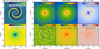 |
Fig. 1 Gravitational potential and acceleration. Left: non-axisymmetric component of the Milky Way external potential. Right: slices through the centre of the galaxy of the acceleration parallel to the Galactic plane in simulations F3000HD (left column) and MW3000HD (middle column) and their relative difference (right column) at t ≈ 2500 Myr. The first row corresponds to the contribution to the acceleration from the external potential, and the second is the contribution from the self-gravity of the gas and the newly created stars. |
3.3 Thermodynamic properties
We have seen that the addition of a barred external potential changes the density structure of the gas in the centre and the amount of supernovae exploding there. In this section we look at how this affects the phase of the gas in different regions of the Galaxy.
In Fig. 3, we show the temperature-density distribution of the conducted simulations for the whole simulation box (left-hand column), the Galactic disc (|z| < 1 kpc and Rgal < 25 kpc, middle column) and the Galactic centre (|z| < 1 kpc and Rgal < 2.5 kpc, right-hand column). Colour coded is the mass fraction of the respective part of the simulation.
The phase plots of the full simulation box show remarkably similar features between simulations: the main bulk of the gas resides in the area of the warm neutral and ionised medium at around T ∼ 104 K, and, at densities larger than 10−24 g cm−3, extends into the cold neutral medium. At densities ≲10−28 g cm−3, gas can only be found in the hot phase, at about 105.5 − 107 K. However, all simulations show hot gas also at densities of 10−28 − 10−23 g cm−3. This is gas recently heated by supernova feedback at its density during the energy injection, which has not yet expanded. When zooming in onto the Galactic disc, the two simulations barely differ. Most of the mass in the hot gas is located in the circumgalactic medium, which explains the small amount of hot low-density gas. Conversely, the amount of gas in the warm and cold phase is hardly reduced compared to the full simulation box, meaning that this gas is mainly found within the Galactic disc. When looking only at the Galactic centre, for both simulations most gas is found in the warm phase. For F3000HD, more gas can be found in the cold phase than for MW3000HD, where instead some hot low-density gas is present. This is a result of higher star formation and supernova rates and denser clustering of star formation and supernova in the Galactic centre, as we show in Sections 4.2, 4.4 and 4.5.
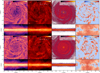 |
Fig. 2 Surface density of total gas (first column), ionised hydrogen (second column), stars (third column), and the temperature in a slice through the midplane (fourth column) for simulations MW3000HD (first row) and F3000HD (second row) for the inner 15 kpc. |
3.4 Radial structure
Given the different overall morphology of our simulated galaxies, one may think that the radially averaged distribution of the gas depends on the proper inclusion of all the components of the Galactic potential. We see here that this is not the case, and that, except in the central region, the flat external potential reproduces fairly well the radial structure of the galaxy modelled with a more complete potential.
In Fig. 4, we present the radial (top row) volume-weighted distribution of gas (left) and newly formed stars (right), averaged over 100 Myr around our fiducial analysis time of 2500 Myr. First, we point out that the density distribution only changes minimally during phase II as we reach a steady state. Second, the radial distribution of the gas is very similar in all of the simulations: a relatively flat distribution, decreasing from ∼10−24 g cm−3 close to the centre to ∼10−25 g cm−3 at the edge of the disc. Gas at these densities is predominantly warm (T ∼ 104 K; see Figure 3), so in all simulations, the volume of the disc is filled primarily with warm neutral and warm ionised gas. The radial distribution of stars is significantly steeper than the gas distribution but is independent of the choice of potential. Within the disc, the density of stars steadily declines towards the Galactic outskirts, with a knee short of 25 kpc and a following, steeper decline (not shown here). We note that there is a noticeable difference between the flat and Milky Way model at a galactocentric distance of 1–3 kpc, both in the gas as well in the stars. This is due to the stronger star formation in the Milky Way model, which manifests in a dip in gas and stellar density at ∼2 kpc, because the centre depletes star-forming material from that zone, and a central peak (<1 kpc) in the distribution of stars.
We emphasise that the depicted curves do not represent the full stellar population present in the simulation boxes, but the one formed after the simulation started (in phase II). The external potential applied to the simulated galaxies provide an additional mass distribution, mainly from (low-mass) stars and DM. For the Milky Way potential (grey dash-dotted curve), the DM component is excluded for comparability (if DM was included, it would dominate the potential at galactocentric radii Rgal > 8.7 kpc). For the flat potential (grey dotted curve), it is not possible to distinguish between gaseous, stellar, and DM components, since it is an analytical potential which describes an overall density distribution. We therefore plotted the distribution of all underlying mass, including possible DM, as determined by the gravitational potential.
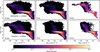 |
Fig. 3 Temperature-density plot for the conducted simulations at the fiducial time of 2500 Myr. All phase plots show a three-phase structure of the ISM, with a hot low-density phase and a colder phase extending to higher densities, and the beginning of a cold phase at densities ρ > 10−24 g cm−3. Some mass is also stored in hot higher density gas, probably because of heating by stellar feedback. |
3.5 Vertical structure
Different vertical accelerations can also result in changes in the vertical mass distributions in the disc. We look at it in the bottom panel of Fig. 4. Again, we find that the vertical distribution of gas density is nearly identical between the two simulations. The stars, however, are not sensitive to pressure gradients. The vertical stellar distribution for MW3000HD is narrower than for F3000HD, i.e. stars are more concentrated towards the Galactic midplane.
We completed this analysis by considering the scale height of the gas and stars, which we define as the height containing 75% of the mass at a given radius. We call this height the ‘75% height’. Again, we average over a timespan of 100 Myr, from 2450 to 2550 Myr. On the left in Fig. 5 we show the 75% height for all mass in the simulation, i.e. gas, newly formed stars and mass in the external potential. There, in grey we also present the height of the stars in the Milky Way potential, i.e. the underlying, not explicitly simulated mass distribution. On the right we show the 75% height for the gas and newly formed stars in the simulation.
The mass distribution of the external potential completely dominates the 75% height for F3000HD (see left panel). The underlying mass distribution of the flat potential is not shown, but identical with the blue solid curve. This is, because the flat potential, as mentioned before, is an analytical potential, and we cannot distinguish between the DM and other components. Therefore, we use the full mass distribution forming the external potential in this figure. As DM is a fuzzy component, it drives the 75% height to higher values. For the Milky Way potential, we remove the DM component for this comparison. MW3000HD is dominated in its 75% height by the underlying potential mass as well (compare grey dash-dot-dotted curve versus solid red curve) up to about 5 kpc. At higher galactocentric radii, however, the simulated mass components lower the 75% height, i.e. they are more closely concentrated to the Galactic disc plane than the mass causing the potential.
In stars and gas, a general trend is present in both simulations of increasing 75% height with increasing Rgal up to a radius of about 10–15 kpc, with a saturation at higher galactocentric radii. For gas, the saturation is about 1 kpc; for stars it is slightly lower, at about 0.5 kpc for both potentials. Stars at Rgal ≳ 10 kpc have a generally lower 75% height than the gaseous component, meaning they are confined closer to the disc than gas. Within the innermost ∼2 kpc, the 75% height of stars shows a bump, caused by local turbulence from close interaction in this region. This, however, is more pronounced in the Milky Way potential, reaching about ∼0.5 dex in height, and is most probably caused by turbulence induced by the bar and the lower potential strength compared to the flat potential (see Fig. 1).
From Eq. (6), it is easy to show that the 75% height x75% is about twice the scale height z by  which results in x75% ≈ 1.94Rzd. Therefore, in MW3000HD in gas we find a scale height at the solar radius of ∼200 pc, and in stars of ∼120 pc. Observed scale heights of the thin and thick stellar disc of the Milky Way are about 140 pc and 400 pc, respectively (see Bland-Hawthorn & Gerhard 2016; Vieira et al. 2023, after transfer into our measure of zd). The scale heights of the stellar disc in our simulation falls close to that of the thin stellar disc, as expected as it consists solely of stars formed during the simulation time. It is even slightly lower; however, our simulated galaxy is dynamically young and lacks interaction with satellite galaxies; the stellar disc would probably increase in scale height if run for a longer time. Ferrière (2001) quotes (exponential) scale heights up to 1000 pc (WIM) for Galactic gas (which corresponds to about 900 pc in sech2). Our found scale height falls well within this limit for the solar circle as well as at the saturation further out in the galaxy.
3.6 Azimuthal structure
The Milky Way external potential is characterised by the presence of two non-axisymmetrical components, the bar and the spiral arm. To have a better idea of how they shape the galaxy, we look at the repartition of the gas and stars in the azimuthal direction at different radii.
Figure 6 shows the azimuthal profile of gas (top panel) and stars (middle panel) at 3–4 kpc, 6–7 kpc and 9–10 kpc. We compare the profile for the simulations F3000HD and MW3000HD. We also plot the contribution of the dominant external non-axisymmetric components of the MW3000HD potential for reference in green and pink. In this plot we focus on the azimuthal fluctuations of each quantities. Each quantity, y, was averaged in azimuthal bins and normalised as follows:

As a result, the plotted value, ynorm, is dimensionless and varies between −0.5 and 0.5.
At all radii, the simulation F3000HD shows no clear large-scale structure, with many peaks in the surface density profiles. On the contrary, the simulation with the Milky Way potential shows fewer peaks that are well correlated with the bar and the spiral arms. The best correlation found are for the stars, where they follow the potential minima of the bar (middle left panel) or the spiral arms (middle right panel). What happens around 6 kpc (middle centre panel) is less clear, as the influence of the bar and the spiral arm are combined.
Overall, our analysis shows that choosing an accurate prescription of the Milky Way potential does not have a big influence on the radial distribution of the gas and young stars, except in the central regions where the bar is prominent. However, the analysis reveal that the bar and the spiral arms have a significant influence on the organisation of the gas and stars in the inner and outer galaxy when looking in the azimuthal direction.
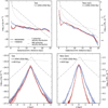 |
Fig. 4 Volume-weighted density distribution of gas (left) and stars (right) in the radial (upper row) and vertical (lower row, averaged from 8 to 9 kpc) directions for F3000HD (blue) and MW3000HD (red) averaged from 2450 to 2550 Myr. Shaded regions indicate the 16th to 84th percentile. The density distributions generating our adopted external potentials are indicated in grey, dotted for the flat potential and dash-dotted for the Milky Way model. In the radial direction, we took into account mass up to z = ±50 pc. |
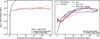 |
Fig. 5 Height of the plane containing 75% of the mass at a given radius for all the simulated mass (left) and the simulated gas and newly formed stars (right) in MW3000HD (red) and F3000HD (blue). In grey, we present height for stars in the Milky Way potential, i.e. the underlying, not explicitly simulated mass distribution. Shaded regions indicate 16th to 84th percentile. In all simulations, stars are more concentrated to the disc plane than gas. |
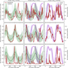 |
Fig. 6 Azimuthal profile of the normalised fluctuations of the gas (top), stars (middle), and SFR (bottom) surface densities at t = 2500 Myr. These are compared with the normalised fluctuations of the contributions of the external non-axisymmetric components of the potential, with the bar (green) and the spirals (pink), associated with the right vertical axis of each panel, which is reversed so that lower values are on top. The data have been averaged over a radius range of 1 kpc, and the shaded area represents the radial variations. |
4 Star formation and stellar feedback
In the previous section, we analysed the effect of an accurate prescription of the Milky Way potential on the morphology of the galaxies, focusing on the gas and star structures. Quite naturally, we expect that a change of the morphology of the gas reflects into a change in where the stars form and the overall star formation properties. In this section, we inspect what is the effect of changing the external potential on the star formation activity, starting from a global point of view and then again refining in the radial and azimuthal directions.
4.1 Global star formation rate is agnostic of potential
We start by looking at the total SFR in our simulations over time in Fig. 7 (left) as well as the gas depletion time (right). We define the SFR as
 (23)
(23)
with tn and tn+1 being the times of two consecutive snapshots, and tn+1 − tn ≈ 5 Myr in our case. The gas depletion time, consequently, is defined by
 (24)
(24)
where  is the arithmetic mean of the gas mass of two consecutive snapshots.
An initial peak is present in both simulations, which results from an initial collapse of the disc when turning off the mass return from supernovae at the end of phase I and the corresponding additional pressure.
Both simulations show very similar global SFRs, declining constantly over the simulation time, which is consistent with the increasing depletion of the gaseous disc by star formation in an isolated galaxy. At our fiducial analysis time, we found SFRs of 2.9 M⊙ yr−1 (F3000HD) and 2.6 M⊙ yr−1 (MW3000HD). These values are at the upper end of estimated SFRs from observations, which mostly suggest a global SFR for the Milky Way of about 1–3 M⊙ yr−1 (see e.g. Chomiuk & Povich 2011; Licquia & Newman 2015; Bland-Hawthorn & Gerhard 2016; Elia et al. 2022, and references therein). At a simulation time of 3000 Myr, the SFR decreased to about 1.5 M⊙ yr−1 (F3000HD), 1.3 M⊙ yr−1 (MW3000HD), which fits observational constraints rather well. From about 3500 Myr of simulation time onward, the SFR is below 1 M⊙ yr−1 and therefore too low for a Milky Way analogue.
The depletion time τ increases during the simulation from less than 103 to more than 104 Myr. The molecular gas depletion time of low redshift main sequence galaxies is found to be between 900 and 2000 Myr (Wang et al. 2022). Our simulations exceed this range after about 2500 Myr. At later simulation times, it therefore seems that the SFE is too low compared to the real Milky Way, possibly because of lack of disturbance of the galaxy by satellites that trigger additional star formation, and because of the fact that we do not model circumgalactic gas that could replenish the Galaxy.
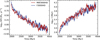 |
Fig. 7 Star formation rate history (left) and depletion time τ (right) for F3000HD (blue) and MW3000HD (red). We limited the measurement to ±1 kpc around the Galactic plane. Changing the potential does not result in a change of the overall SFR at the fiducial analysis time. |
4.2 Radial distribution of star formation
Since the global SFR is nearly identical for both potentials, in Fig. 8 we present the SFR surface density ΣSFR in radial bins for the Galactic centre (top row) and the whole disc (bottom row). Again, a constant decline in ΣSFR is present at all radii, except the outermost bin of 20–30 kpc. The Galactic outskirts remain at a constant, but low ΣSFR. Comparing values for the whole disc in F3000HD and MW3000HD, the ΣSFR at different radial bins largely agrees apart from the innermost 6 kpc. For F3000HD, star formation in this region declines steeply with time, with the SFR of the centre falling below the average SFR of the rest of the disc about halfway through phase II. Conversely, in run MW3000HD, ΣSFR does not decline below the levels of regions further out. This most probably is because of the constant channeling of gas into the Galactic centre by the bar, which prevents quenching. Soon after the beginning of phase II, ΣSFR is rather constant from 6 up to 20 kpc, i.e. the corresponding curves overlap to a large degree.
Zooming in onto the Galactic centre (two left panels), differences in the distribution of star formation become more apparent. Whereas for F3000HD, star formation is mostly evenly distributed throughout the innermost 6 kpc (ΣSFR agrees for different radial bins) and is lowest for the innermost 1.5 kpc, a clear trend in ΣSFR is visible for MW3000HD. We find the highest ΣSFR within the innermost 1.5 kpc. Between 3–4.5 and 4.5–6 kpc, ΣSFR is roughly the same, with a value ∼0.5 dex below the value in the innermost bin. Between 1.5 and 3 kpc, far fewer stars are formed than at smaller radii. After about 2500 Myr, ΣSFR in this region is comparable to or lower than the SFR density at R > 20 kpc, i.e. this zone is quenched. However, from 0 to 1.5 kpc star formation does not quench during the duration of the simulation. This is most probably prevented by constant gas inflow into the centre due to gas dynamics in the bar. Fig. 10a shows this in more detail, as we explain in Section 4.3.
On the other hand, F3000HD shows a severe drop off and even a complete stop of star formation after about 3000 Myr. Whereas ΣSFR is lowest within 1.5 kpc galactocentric radius for most of the simulation time, star formation does not fully stop there at any time. Instead, it continues on a low and constant level from 2500 Myr onward.
We therefore conclude that gas streaming due to bar dynamics has a large influence on star formation in the centre of the galaxy. For a better understanding of this channeling of mass to the galactic centre by the bar, we present the enclosed mass over time within different radii (normalised to the enclosed mass at the beginning of phase II) in Fig. 9. The enclosed mass in the inner 1.5 kpc of MW3000HD increases by about 50% during the simulation time, whereas in F3000HD it varies very little. Most of the channeled mass comes from within the bar-dominated region, as the enclosed mass within 6 kpc varies by less than 10%. This clearly shows the redistribution of mass conducted by the bar potential.
4.3 Azimuthal distribution of star formation
While both simulations have spiral arms and show a similar SFR radial profile outside the central region, we have seen in Section 3.6 that the Milky Way external potential has a strong influence on the azimuthal distribution of the gas and stars. It is thus interesting to look at the azimuthal distribution of the SFR, which we do in the bottom row of Fig. 6. Again, we look at radial bins from 3–4 kpc (left), 6–7 kpc (middle) and 9–10 kpc (right), for F3000HD (blue) and MW3000HD (red), together with the Milky Way potential for the bar (green) and the spiral arms (pink). The value of the SFR is also normalised as described in Section 3.6. As we can expect, the SFR in F3000HD shows no periodicity in the azimuthal direction at any given radius. On the other hand, the SFR in MW3000HD correlates well with low points in the dominating potential pattern, be it the bar (see left panel) or the spiral arms (see right panel). Within those potential wells, SFR is increased. In regions with no strong dominance of one potential pattern over the other (central panel), SFR presents no clear correlation with one or the other of the given potential patterns.
To expand this analysis and see if it is robust at different time step, we need to look at where star formation occurs over time. To that purpose, we use rotation corrected R–Φ-projection indicating the total stellar mass formed in different regions of the galaxy (Fig. 10). The figure spans the whole time of our simulation (phase II) and is corrected for rotation with the pattern speed of the Galactic bar (top-left panel) and spiral arms (top-middle panel). In the top-left panel we do not see a clear pattern in where stars are forming for Rgal ≳ 4.5 kpc, as bar and spiral potentials with different pattern speeds overlap in this region (as already seen in Fig. 6). However, between 1 and 3 kpc star formation is located within streams of gas to the Galactic centre and circular active star formation zones at their tips (see contour lines). In the top-middle panels we show the disc region of MW3000HD, with non-spiral arm regions crossed out. For this purpose, we define spiral arms as regions where the non-axisymmetric spiral arm potential perturbation is lower than 0 m2 s−2. As in Fig. 6, we find that star formation occurs preferentially within the spiral arms. At radii > 14 kpc, however, these star formation regions get out of sync with the inter-arm regions, because the rotational speed of the gas drops below the pattern speed. This is also evidence that the Milky Way external potential yield long-lived spiral structure where star formation occurs preferentially. To quantify this, in Fig. 10 (upper right) we present the mass fraction of stars formed within spiral arms versus galactocentric distance. For 6 kpc ≤ Rgal ≤ 16 kpc, more than half of all stellar mass is built within spiral arms, with a peak of 70–75% between 9 and 14 kpc. Outside of 14 kpc, the fraction of stellar mass formed within spiral arms drops off steeply and reaches an equal distribution between arm and interarm regions at about 16 kpc. This, as mentioned before, is most likely caused by the discrepancy between the rotation speed of the gas, which slowly declines with radius and the pattern speed of the spiral arm potential, which behaves similar to a solid body. In total, of all stars formed beyond 6 kpc, about 62% are formed in spiral arms.
Contrary to the Milky Way Model, for F3000HD (lower row of Fig. 10) we do not find similar noticeable features. Spiral structures do emerge in this simulation as well (see Fig. 2) but they do not persist over time. Indeed, we produced a series of rotation-corrected R–Φ-projection with angular frequency ranging from 15 to 35.0 km s−1 kpc−1 in steps of 0.5 km s−1 kpc−1, of which three examples are shown (Ω = 15, 26 and 35 km s−1 kpc−1). We did not see any coherent spiral pattern in any of the tested angular frequency Ω.
We have seen in Section 4.1 that the global SFR is similar in both sets of runs. That suggests that although differences in the potential clearly influence where stars form, they make little difference to the galaxy-averaged SFE. This is consistent with prior theoretical and observational work. For example, Kim et al. (2020) simulated a local patch of the ISM with an imposed spiral potential and found that while star formation occurs preferentially in the spirals, where the gas is denser, the SFE is not enhanced by the spiral perturbation. On the observational side, comparisons of the SFE in spiral arms with the efficiency in inter-arm regions in our Milky Way (Ragan et al. 2018) and other nearby spiral galaxies (Sun et al. 2023; Querejeta et al. 2024) find little or no systematic difference.
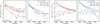 |
Fig. 8 Star formation rate surface density in MW3000HD and F3000HD in radial bins for the central (Rgal < 6 kpc) region (two left-hand panels) and whole disc (two right-hand panels). |
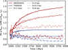 |
Fig. 9 Total mass enclosed in 1.5 kpc, 3 kpc, 4.5 kpc, and 6 kpc normalised by the initial mass within this radius at the beginning of phase II (time t0) for F3000HD (blue) and MW3000HD (red). For MW3000HD we find an increase of about 50% in enclosed mass in the innermost 1.5 kpc. |
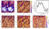 |
Fig. 10 Stellar mass fraction formed in spirals in MW3000HD (top-right panel) and formed stellar mass in the Rgal – Φ-projection for the MW3000HD disc region (6 kpc ≤ Rgal < 20 kpc, top-middle panel) and bar region (Rgal < 6 kpc, top-left panel), corrected for the corresponding pattern rotation, as well as for the disc region of F3000HD, corrected for a pattern speed of Ω = 15.0, 26.0 and 35.0 km s−1 kpc−1 (bottom row). Contour lines indicate 10%, 30%, and 50% of the maximum stellar mass formed (excluding the region of extremely high formed stellar mass at < 0.1 kpc for MW3000HD bar region, upper left). For the MW3000HD disc region, the upper-middle interarm regions are shaded out. |
4.4 Clustering of star formation
In Sections 4.2 and 4.3, we found an increased concentration of star formation activity towards the Galactic centre and a more coherent azimuthal distribution of star formation over time in MW3000HD compared to F3000HD. This raises the question of whether in those regions of increased star formation the star particles also form in a more clustered manner. From observations and theoretical predictions, we know that clustered star formation and the resulting clustered feedback have the potential to strongly influence the appearance of galaxies (e.g. by creating bubbles and outflows; see e.g. Ferrière 2001; Crocker & Aharonian 2011; Crocker 2012). As we observed such changes in our simulations (see Girichidis et al., in prep.), we are interested in any changes induced to clustering of star formation and stellar feedback (which we study in Section 4.5) by differences in the potentials. In this section, we therefore study the abundance of clustered star formation as well as the properties of such clusters.
For this analysis we use the python clustering library HDB-SCAN (Campello et al. 2013). HDBSCAN, together with other clustering algorithms, was tested on Gaia data to detect open clusters in five dimensional space of coordinates, proper motion and parallax by Hunt & Reffert (2021). It was found to have highest sensitivity of the tested algorithms and in general to work best for Gaia data. HDBSCAN is a hierarchical clustering algorithm and is able to find clusters in regions of vastly different densities, utilising a minimum spanning tree weighted by nearest-neighbour distances. Via single-linkage, it is then checked if the termination of a single connection would divide a cluster into two clusters, each with a number of members greater than a predefined number (min_cluster_size), or if the point would be merely falling out of the cluster. In the first case, the new clusters are kept as individual clusters, and in the latter case, the cluster keeps its structure. The result is a cluster hierarchy from which the flat clustering is then derived by checks for stability of the clusters, again based on the weighted distances. HDB-SCAN therefore does not utilise some predefined density threshold or similar, but instead finds stable overdensities compared to the local background. The algorithm is controlled by the single parameter min_cluster_size mentioned before, and it sets the lowest number of members a cluster can have. In our analysis, we set the parameter min_cluster_size to five (even though we varied this parameter between three and seven to indicate variance in the outcome due to the used algorithm), i.e. we did not take into account any associations with fewer than five star particles. We are looking for groups in a four dimensional space of birth coordinates and birth time, so star particles identified to be in the same group have to be formed in close spatial vicinity and soon after each other. The found groups have very similar distributions in the number of group members across simulations and galaxy regions, ranging from the defined minimum number of five to several hundreds of star particles. The median number of group members is ten and therefore well above the selected minimum number. If the selected min_cluster_size is smaller, the found clusters tend to be smaller naturally, if it is larger the cluster size tends to be larger (see Figs. 11 and 12). This is because a lower min_cluster_size allows for fragmentation into smaller subgroups, whereas a higher min_cluster_size prevents such fragmentation. However, we find the change in min_cluster_size to not change the overall picture.
We are simply interested in the properties of regions where stars are not formed in isolation, where those regions are, what their size is, and for how long they last. Therefore, we do not name the found structures ‘clusters’ but simply ‘groups’, as ‘cluster’ is a widely used term in the astronomical context. However, the associations found with HDBSCAN are not meant to resemble stellar clusters, as each star particle itself already represents several (massive) stars (see Sections 2.6 and 2.7).
We present our findings for different regions of the simulated galaxies in Fig. 11. From left to right, we selected different radial ranges: Rgal ≤ 2.5 kpc (left), Rgal ≤ 5 kpc (middle), Rgal > 5 kpc (right). Because of the aforementioned similar distribution in the number of group members and because star particles in our simulations have little spread in mass, the mass distributions of groups are also very similar (see Fig. 11, first row) across simulations and Galactic regions. They range from about 104 to 106 M⊙, with a median at about 104.5 Msun and a tail towards higher masses (when a different min_cluster_size is used the distributions are changed according to the aforementioned effects).
We also present the stellar mass fraction born in groups  (Fig. 11, second row). We find that in general more than 50% of the stellar mass is formed in groups, for the innermost 5 kpc ranging between ∼50% to ∼70%, and being relatively stable at around 65% in the disc region (with large statistical fluctuations at the Galactic outskirts). In the inner 5 kpc of F3000HD we can see an increasing grouping with radius, but no clear trend for MW3000HD, and also no enhanced grouping in star formation is present in Galactic spirals, as one might expect. At Rgal > 100.5 kpc in all used min_cluster_size more stellar mass is formed in groups than outside of groups. We therefore conclude clustering to be a ubiquitous phenomenon present at a comparable fraction in all regions of the Galaxy.
In the third row of Fig. 11, we present the activity time tgroup of the group, which is calculated as the difference between the birth time of the first and last star particle of the group. It therefore represents the time over which a star-forming region actively forms star particles. Star-forming regions with activity times lower than the global time step we group together in the lowest bin depicted. In the activity times, differences between the Galactic regions are present: the median activity time increases with galactocentric distance, being larger in the Galactic disc than in the central region. This means that star-forming regions consisting of multiple star-forming cells persist for longer in the Galactic disc than in the centre. Finally, we also find a difference between Galactic models in the Galactic centre, with groups in the innermost 2.5 kpc (i.e. in the inner bar region) of MW3000HD having an about 0.2 dex lower activity time than in F3000HD, whose distribution shows a tail towards long activity times. This might be caused by stronger turbulent forces and shear, which we know to influence SFRs (e.g. Colling et al. 2018) and turbulence because of the bar potential in MW3000HD. Another possible explanation is that because of the higher SFR in the centre of MW3000HD, star-forming regions are depleted of their star-forming gas faster than in F3000HD.
Another consequence of the presence of a galactic bar is the prevalence of smaller groups in the centre of MW3000HD than in F3000HD (see Fig. 11, last row). ‘Smaller‘ here means a lower occupied cuboid volume Vgroup = (max(x) – min(x)) (max(y) – min(y))(max(z) − min(z)) (compared to the large dynamical range of 10 orders of magnitude, the actual measure of the occupied volume, be it cuboid, spherical or a convex hull, is negligible). The median extent in MW3000HD within the innermost 2.5 kpc is about 0.5 dex lower than in F3000HD, with a noticeable tail towards low volumes. In the Galactic disc, no such difference between simulations is present, and median group extends are up to 1 dex more extended than in the Galactic centre.
In summary, the star clustering properties are heavily affected by the external potential in the central region, where the groups of stars are more compact and form faster in the Milky Way than the flat potential. On the other hand, the groups of stars formed outside the central regions have the same statistical properties, and thus these properties do not depend on the external potential.
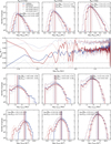 |
Fig. 11 Grouped star formation: mass of group (first row), mass fraction of stars born in groups (second row), activity time (third row), and volume of groups (fourth row) for F3000HD (blue) and MW3000HD (red) in the Galactic centre (≤2.5 kpc, left column), inner region (≤5 kpc, middle column), and disc (>5 kpc, right column). Vertical lines indicate median values, which are written out at the upper left or right. Faint lines indicate distributions and medians for a min_cluster_size of three (dashed) and seven (dotted). The corresponding median values are given in brackets. |
4.5 Clustering of supernova feedback
As soon as star particles formed from the gas, they are decoupled from the hydrodynamic flow and are subject just to gravitational forces. This increases the impact the gravitational potential has on their motion, making stellar feedback, as it is just tied to the dynamics of star particles, an interesting probe of the Galactic potential. Moreover, supernovae exploding in groups have a substantial impact on their surrounding environment, as they can form superbubbles and strong galactic outflows, which is not possible for individual supernovae. The clustering of star formation and stellar feedback of course will be heavily influenced by the exact implementation of the star formation model and early feedback (or lack thereof). However, since we are interested in differences induced by changes in the galactic potential, and the named implementations are identical for both conducted simulations, we leave the examination of such effects to future studies.
Because of the high number of supernova explosions (each star particle can hold several massive stars that explode as supernovae), we can only perform the analysis for a limited time, which we choose to be 2450–2550 Myr. While we find strictly more than 50% of stellar mass being formed in groups in the Galactic centre, the number fraction of supernova exploding in groups in the centre (5 kpc ≈ 100.7 kpc) is very volatile and ranges from 0 to about 60% (see Fig. 12, second row). Further out, the fraction falls below 50% (where it is about 65% for stars formed). This does not differ between MW3000HD and F3000HD. This suggests that groups are ripped apart in between the formation of stars and the explosion times of supernovae. In the innermost 1 kpc, supernovae are grouped to a lower degree in space and time in MW3000HD than in F3000HD (for this small radius we were able to check grouping for a longer times-pan, giving a more clear result, but we show data of the selected timespan here for consistency). This shows that a barred potential is necessary to get the right clustering of stellar feedback in the Galactic centre.
As for star particles, groups of supernovae in the centre of MW3000HD experience shorter activity times than in F3000HD (∼0.54 dex), whereas activity times do not differ in the Galactic disc > 5 kpc (third row; again we collect all clusters with an activity time below the global time step of the simulation in the lowest bin). In the disc the median activity time of supernova regions is also 0.2–0.3 dex lower than for star particle groups.
Supernova groups in the Galactic centre have about 0.7 dex smaller median extent in MW3000HD than in F3000HD, with the size distribution of MW3000HD showing a similar, but even stronger bimodal pattern than observed for the star particles. In the disc, no such difference is present. Extends of supernova groups in general are slightly lower than those of star particle groups.
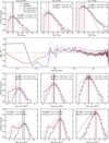 |
Fig. 12 Grouped supernovae: number of association members (top row), fraction of supernova exploding within groups (second row), activity time (third row), and extend of groups (fourth row) for F3000HD and MW3000HD for t = 2450–2550 Myr. Vertical lines indicate median values. Faint lines indicate distributions and medians for a min_cluster_size of 3 (dashed) and 7 (dotted). Corresponding median values are given in brackets. |
5 Discussion and conclusions
5.1 Caveats
Some of the presented results reveal shortcomings of our simulations. However, these can never be fully avoided in simplified models of complex systems.
The global SFR, for example, shows a continuous decline over the simulated time. In order to study the prevailing processes in our simulations precisely, we did not wish to account for gas accretion onto the Galactic disc, and we therefore modelled our Galaxies without a circumgalactic medium. The only gas accretion onto the ISM is therefore previously expelled gas from the Galactic disc. The lack of an additional supply of fresh gas, however, results in a progressive depletion of gas in the simulation, as gas gets converted into star particles. This, in part, is a desired result, but it also leads to a limited time over which the results are directly comparable to the Milky Way. The lack of gas at late times also results in an SFR below the typical Milky Way value of 1 M⊙ yr−1.
The isolated galaxy approach also resulted in a lack of satellites for our Milky Way analogues. The observed Milky Way has multiple smaller satellite galaxies, with the Large and Small Magellanic Clouds being the largest, which influence the Galactic dynamics (see e.g. Correa Magnus & Vasiliev 2022) as well as the evolution history (e.g. Sotillo-Ramos et al. 2022 and Malhan et al. 2022). In today’s Milky Way observations, past mergers are still present as stellar streams or globular clusters. This lack of companions (as well as a low age) might be the reason for the thinness of the stellar and gaseous disc in our simulations.
In addition, we also ignored pre-supernova feedback such as photoionisation and stellar winds in our simulations. This might impact the ISM structure in terms of increasing the amount of ionised gas. However, we plan to include them in future work.
In this paper, we focused on the hydrodynamic simulations while omitting magnetic fields and cosmic rays, as both processes are known to have an impact on the star formation and the dynamics of the ISM. Simulations including magnetic fields and cosmic rays will be discussed in companion papers (Kjellgren et al. 2025, Girichidis et al., in prep.).
5.2 This work in context
In this work, we have examined the influence of the gravitational potential of a galaxy on its star formation. We find significant effects of the bar potential on the amount and distribution of stars formed in its region of influence. This is in line with findings from other simulation and observational works. The Galactic bar channels gas into the galactic centre, aiding star formation at Rgal < 1 kpc and depleting gas further out. This was found in several other studies of simulations, such as Seo & Kim (2013); Armillotta et al. (2019); Tress et al. (2020b), and Sormani et al. (2020). These, however, only modelled the bar region of the Galaxy without taking into account the full galactic context. The importance of the full galactic environment was shown, for example, in Pettitt et al. (2020), who ran several simulations with different combinations of bar and spiral arm potentials. They find a small burst in star formation when the bar overtakes the spiral arms, showing the interplay between the two components. Seo et al. (2019) have shown the correlation between the bar and the rest of the galactic disc by simulating it in discs of different velocity dispersion and gas fraction. Both simulations also find an influence of the bar on spurs in the galactic disc. This, again, emphasises the cross-correlation between different features of the Galaxy.
Several simulations modelling the full Galactic disc, however, ignore the bar potential (e.g. Pettitt et al. 2014; Jeffreson et al. 2020; Wibking & Krumholz 2023; Konstantinou et al. 2024). As spiral features emerge even without an explicit gravitational potential dedicated to them via sheering of overdense regions, they appear in numerous simulations modelling the full galactic disc. This work, however, shows clear differences in the lifetime of self-appearing or build-in spirals, which influences the amount of star formation in spiral arms but not the overall SFR in this work (even though a complete suppression of the formation of spiral arms decreases the SFR in a galaxy; see Robinson et al. 2025). Star formation in spiral arms is studied in stratified box simulations (e.g. Kim et al. 2020) or simulations of incomplete galactic discs (Smith et al. 2020). If the full disc is simulated, the bar potential is often ignored (Dobbs et al. 2011). Thus, the dynamical interplay between different regions of the galaxy is lost. Moreover, a bar potential itself can induce spiral features in a galactic disc (Pettitt et al. 2020). While many questions of star formation in spiral arms – such as if the SFE is increased in the arm potential – can be examined in simulations of the arms alone; interactions of the potentials of the Galactic bar and spiral arms are not modelled. Moreover, where the dominance of the Galactic bar begins in the inner disc, star formation in spiral arms are truncates, while without a bar, they reach close to the centre of the galaxy (see Pettitt et al. 2020).
In this work, we have modelled both non-axisymmetric components, the bar, and spiral arms together with axisymmetric gravitational features in a way that is fitted to many observational properties of the observed Milky Way (see Hunter et al. 2024). The gravitational dominance in different regions of the disc was tracked reliably, aiding in representing a realistic distribution of star formation that is missing in simulations that include only one or the other component. The comparison with a simple flat potential enables an estimate of where these potential features are of importance in the distribution of star formation and where a more simplified potential is sufficient. Instead of presenting a general study of different potential features, i.e. two versus four spiral arms, weak bar versus strong bar, we show a characterisation of a specified (and not generalised) Milky Way potential.
5.3 Conclusions
In this work, we have introduced the Rhea simulation suite, a set of comparable simulations of Milky Way-like galaxies with varying external potentials. We considered a detailed external potential tuned to re-create observations of morphology and dynamics of the Milky Way and compared it to a simple potential with a flat velocity curve. We focused on the morphological and dynamical differences induced by the potential and the related impact on star formation and stellar feedback.
We find that the details of the potential strongly influence where stars form within the galaxy. On the other hand, global SFR properties are only mildly affected. It was therefore sufficient to use a simplified axisymmetric potential to reproduce the global SFR and galactic gas depletion time.
The Milky Way potential most strongly affects the star formation in the galactic centre. The bar results in continuous fueling of the central zone, increases the local SFR by up to an order of magnitude, and favours the formation of compact star-forming groups. Furthermore, the spiral potential produces long-lived star-forming spiral arms, contrary to the transient spirals emerging in the flat potential. Consequently, for an accurate model of the Milky Way, a detailed potential is of crucial importance.
The Milky Way potential, particularly the bar, prevents the Galactic centre from quenching over time. Inside a radius of 6 kpc, following an initial transient, the SFR density declines by around 1.5 orders of magnitude over a timescale of 2 Gyr in the simulation with the Milky Way potential but by more than three orders of magnitude in the simulation with the flat potential. In the Milky Way simulation, the star formation is strongly centrally concentrated and strongest in the innermost 1.5 kpc. About 5.3% of all stars in the galaxy are born within this radius. On the other hand, in the flat potential model, only 3.8% of star formation occurs within the same radius.
With the Milky Way potential, the density of gas, stars, and hence star formation tend to increase in the potential wells of the spiral arms and bar. Approximately 60% of stars outside the bar region form within spiral arms. Such a pattern is not observable with the flat external potential, as no long-lived star-forming spiral patterns form. The transient spirals that form with the flat potential show no consistent pattern speed.
About 60–65% of star particles form close to other star particles in groups in both simulations. Compared to a non-barred potential, in the bar potential the lifetime and size of those associations is lowered by ∼0.2 dex and ∼0.5 dex, respectively.
For all radii the fraction of supernovae that explode in isolation is about 50%. Compared to the flat potential, the activity times and sizes of associations of supernovae are lowered in the central region of the Milky Way potential by ∼0.5 dex and ∼0.7 dex, respectively.
In future work, we will extend the Rhea simulations to include magnetic fields and cosmic rays (CRs), enabling a quantitative assessment of their influence on star formation and feedback in a self-consistent Galactic context. These extensions will provide an important step toward a fully dynamic model of the Milky Way (MW) interstellar medium.
Our findings reveal which regions of the galaxy respond most sensitively to the detailed form of the gravitational potential. This provides guidance for future models by identifying where a precise description of the potential is essential for understanding star-formation processes, and where a simplified approximation already captures the relevant physics.
Acknowledgements
We thank the referee for a careful reading of the manuscript and constructive comments that helped improving the paper. This research was funded by the European Research Council via the ERC Synergy Grant “ECO-GAL” (project ID 855130). The team in Heidelberg acknowledges support from the German Excellence Strategy via the Heidelberg Cluster of Excellence (EXC 2181 – 390900948) “STRUCTURES”, and from the German Ministry for Economic Affairs and Climate Action in project “MAINN” (funding ID 50OO2206). The authors gratefully acknowledge the scientific support and HPC resources provided by the Erlangen National High Performance Computing Center (NHR@FAU) of the Friedrich-Alexander-Universität Erlangen-Nürnberg (FAU) under the NHR project a104bc. NHR funding is provided by federal and Bavar-ian state authorities. NHR@FAU hardware is partially funded by the German Research Foundation (DFG) – 440719683. They also thank for computing resources provided by the Ministry of Science, Research and the Arts (MWK) of the State of Baden-Württemberg through bwHPC and the German Science Foundation (DFG) through grants INST 35/1134-1 FUGG and 35/1597-1 FUGG, and for data storage at SDS@hd funded through grants INST 35/1314-1 FUGG and INST 35/1503-1 FUGG. NB acknowledges support from the ANR BRIDGES grant (ANR-23-CE31-0005). NB also gratefully acknowledges support from the CBPsmn (PSMN, Pôle Scientifique de Modélisation Numérique) of the ENS de Lyon for the computing resources. MCS acknowledges financial support from the European Research Council under the ERC Starting Grant “GalFlow” (grant 101116226) and from Fondazione Cariplo under the grant ERC attrattività no. 2023-3014. JG, KK and GH are fellows of the International Max Planck Research School for Astronomy and Cosmic Physics at the University of Hei-delberg (IMPRS-HD). RSK is grateful for support from the Harvard Radcliffe Institute for Advanced Studies and Harvard-Smithsonian Center for Astrophysics for their hospitality and support during his sabbatical. JG wants to thank Matthew Smith, Rüdiger Pakmor and David Whitworth for helpful and insightful discussions. For this work, we used astropy (Astropy Collaboration 2013, 2018, 2022), yt (Turk et al. 2011), numpy (Harris et al. 2020), matplotlib, scipy (Virtanen et al. 2020), AGAMA (Vasiliev 2019) and Arepo (Springel 2010).
References
- Agertz, O., Renaud, F., Feltzing, S., et al. 2021, MNRAS, 503, 5826 [NASA ADS] [CrossRef] [Google Scholar]
- Armillotta, L., Krumholz, M. R., Di Teodoro, E. M., & McClure-Griffiths, N. M. 2019, MNRAS, 490, 4401 [NASA ADS] [CrossRef] [Google Scholar]
- Astropy Collaboration (Robitaille, T. P., et al.) 2013, A&A, 558, A33 [NASA ADS] [CrossRef] [EDP Sciences] [Google Scholar]
- Astropy Collaboration (Price-Whelan, A. M., et al.) 2018, AJ, 156, 123 [Google Scholar]
- Astropy Collaboration (Price-Whelan, A. M., et al.) 2022, ApJ, 935, 167 [NASA ADS] [CrossRef] [Google Scholar]
- Benedettini, M., Molinari, S., Baldeschi, A., et al. 2020, A&A, 633, A147 [NASA ADS] [CrossRef] [EDP Sciences] [Google Scholar]
- Benjamin, R. A., Churchwell, E., Babler, B. L., et al. 2005, ApJ, 630, L149 [NASA ADS] [CrossRef] [Google Scholar]
- Beuther, H., Bihr, S., Rugel, M., et al. 2016, A&A, 595, A32 [NASA ADS] [CrossRef] [EDP Sciences] [Google Scholar]
- Binney, J., & Tremaine, S. 2008, Galactic Dynamics, 2nd edn. (Princeton University Press) [Google Scholar]
- Bland-Hawthorn, J., & Gerhard, O. 2016, ARA&A, 54, 529 [Google Scholar]
- Blondin, J. M., Wright, E. B., Borkowski, K. J., & Reynolds, S. P. 1998, ApJ, 500, 342 [Google Scholar]
- Brunthaler, A., Menten, K. M., Dzib, S. A., et al. 2021, A&A, 651, A85 [EDP Sciences] [Google Scholar]
- Buck, T., Obreja, A., Macciò, A. V., et al. 2020, MNRAS, 491, 3461 [Google Scholar]
- Cabrera-Lavers, A., González-Fernández, C., Garzón, F., Hammersley, P. L., & López-Corredoira, M. 2008, A&A, 491, 781 [NASA ADS] [CrossRef] [EDP Sciences] [Google Scholar]
- Campello, R. J. G. B., Moulavi, D., & Sander, J. 2013, in Advances in Knowledge Discovery and Data Mining, eds. J. Pei, V. S. Tseng, L. Cao, H. Motoda, & G. Xu (Berlin, Heidelberg: Springer Berlin Heidelberg), 160 [Google Scholar]
- Carey, S. J., Noriega-Crespo, A., Mizuno, D. R., et al. 2009, PASP, 121, 76 [Google Scholar]
- Chomiuk, L., & Povich, M. S. 2011, AJ, 142, 197 [Google Scholar]
- Clark, P. C., Glover, S. C. O., & Klessen, R. S. 2012, MNRAS, 420, 745 [NASA ADS] [CrossRef] [Google Scholar]
- Clark, P. C., Glover, S. C. O., Ragan, S. E., & Duarte-Cabral, A. 2019, MNRAS, 486, 4622 [Google Scholar]
- Colling, C., Hennebelle, P., Geen, S., Iffrig, O., & Bournaud, F. 2018, A&A, 620, A21 [NASA ADS] [CrossRef] [EDP Sciences] [Google Scholar]
- Correa Magnus, L., & Vasiliev, E. 2022, MNRAS, 511, 2610 [NASA ADS] [CrossRef] [Google Scholar]
- Crocker, R. M. 2012, MNRAS, 423, 3512 [Google Scholar]
- Crocker, R. M., & Aharonian, F. 2011, Phys. Rev. Lett., 106, 101102 [Google Scholar]
- Dobbs, C. L., Burkert, A., & Pringle, J. E. 2011, MNRAS, 417, 1318 [NASA ADS] [CrossRef] [Google Scholar]
- Dobler, G., Finkbeiner, D. P., Cholis, I., Slatyer, T., & Weiner, N. 2010, ApJ, 717, 825 [Google Scholar]
- Draine, B. T. 1978, ApJS, 36, 595 [Google Scholar]
- Drimmel, R. 2000, A&A, 358, L13 [NASA ADS] [Google Scholar]
- Durán-Camacho, E., Duarte-Cabral, A., Pettitt, A. R., et al. 2024, MNRAS, 532, 126 [Google Scholar]
- Elia, D., Molinari, S., Schisano, E., et al. 2022, ApJ, 941, 162 [NASA ADS] [CrossRef] [Google Scholar]
- Elias, L. M., Sales, L. V., Creasey, P., et al. 2018, MNRAS, 479, 4004 [Google Scholar]
- Fattahi, A., Navarro, J. F., Sawala, T., et al. 2016, MNRAS, 457, 844 [NASA ADS] [CrossRef] [Google Scholar]
- Ferrière, K. M. 2001, Rev. Mod. Phys., 73, 1031 [NASA ADS] [CrossRef] [Google Scholar]
- Foyle, K., Rix, H. W., Walter, F., & Leroy, A. K. 2010, ApJ, 725, 534 [NASA ADS] [CrossRef] [Google Scholar]
- Gaia Collaboration (Vallenari, A., et al.) 2023, A&A, 674, A1 [NASA ADS] [CrossRef] [EDP Sciences] [Google Scholar]
- Gatto, A., Walch, S., Low, M. M. M., et al. 2015, MNRAS, 449, 1057 [NASA ADS] [CrossRef] [Google Scholar]
- Gensior, J., Feldmann, R., Mayer, L., et al. 2023, MNRAS, 518, L63 [Google Scholar]
- Gerola, H., & Seiden, P. E. 1978, ApJ, 223, 129 [Google Scholar]
- Girichidis, P., Offner, S. S. R., Kritsuk, A. G., et al. 2020, Space Sci. Rev., 216, 68 [NASA ADS] [CrossRef] [Google Scholar]
- Glover, S. C. O., & Mac Low, M.-M. 2007a, ApJS, 169, 239 [Google Scholar]
- Glover, S. C. O., & Mac Low, M.-M. 2007b, ApJ, 659, 1317 [Google Scholar]
- Glover, S. C. O., & Clark, P. C. 2012, MNRAS, 421, 116 [NASA ADS] [Google Scholar]
- Glover, S. C. O., Federrath, C., Mac Low, M. M., & Klessen, R. S. 2010, MNRAS, 404, 2 [Google Scholar]
- Grand, R. J. J., Gómez, F. A., Marinacci, F., et al. 2017, MNRAS, 467, 179 [NASA ADS] [Google Scholar]
- Harris, C. R., Millman, K. J., van der Walt, S. J., et al. 2020, Nature, 585, 357 [NASA ADS] [CrossRef] [Google Scholar]
- Hou, L. G., & Han, J. L. 2014, A&A, 569, A125 [NASA ADS] [CrossRef] [EDP Sciences] [Google Scholar]
- Hunt, E. L., & Reffert, S. 2021, A&A, 646, A104 [NASA ADS] [CrossRef] [EDP Sciences] [Google Scholar]
- Hunter, G. H., Sormani, M. C., Beckmann, J. P., et al. 2024, A&A, 692, A216 [NASA ADS] [CrossRef] [EDP Sciences] [Google Scholar]
- Immer, K., Schuller, F., Omont, A., & Menten, K. M. 2012, A&A, 537, A121 [NASA ADS] [CrossRef] [EDP Sciences] [Google Scholar]
- Jeffreson, S. M. R., Kruijssen, J. M. D., Keller, B. W., Chevance, M., & Glover, S. C. O. 2020, MNRAS, 498, 385 [Google Scholar]
- Joshi, P. R., Walch, S., Seifried, D., et al. 2019, MNRAS, 484, 1735 [Google Scholar]
- Kalberla, P. M. W., & Dedes, L. 2008, A&A, 487, 951 [NASA ADS] [CrossRef] [EDP Sciences] [Google Scholar]
- Kennicutt, R. C., & Evans, N. J. 2012, ARA&A, 50, 531 [NASA ADS] [CrossRef] [Google Scholar]
- Kim, C.-G., & Ostriker, E. C. 2015, ApJ, 802, 99 [NASA ADS] [CrossRef] [Google Scholar]
- Kim, W.-T., Kim, C.-G., & Ostriker, E. C. 2020, ApJ, 898, 35 [Google Scholar]
- Kjellgren, K., Girichidis, P., Göller, J., et al. 2025, A&A, 700, A124 [NASA ADS] [CrossRef] [EDP Sciences] [Google Scholar]
- Konstantinou, A., Ntormousi, E., Tassis, K., & Pallottini, A. 2024, A&A, 686, A8 [NASA ADS] [CrossRef] [EDP Sciences] [Google Scholar]
- Kroupa, P. 2001, MNRAS, 322, 231 [NASA ADS] [CrossRef] [Google Scholar]
- Kruijssen, J. M. D., Longmore, S. N., Elmegreen, B. G., et al. 2014, MNRAS, 440, 3370 [Google Scholar]
- Li, Q., Narayanan, D., Torrey, P., Davé, R., & Vogelsberger, M. 2021, MNRAS, 507, 548 [NASA ADS] [CrossRef] [Google Scholar]
- Licquia, T. C., & Newman, J. A. 2015, ApJ, 806, 96 [NASA ADS] [CrossRef] [Google Scholar]
- Lin, C. C., & Shu, F. H. 1964, ApJ, 140, 646 [Google Scholar]
- Longmore, S. N., Bally, J., Testi, L., et al. 2013, MNRAS, 429, 987 [NASA ADS] [CrossRef] [Google Scholar]
- Mackey, J., Walch, S., Seifried, D., et al. 2019, MNRAS, 486, 1094 [Google Scholar]
- Maeder, A. 2008, Physics, Formation and Evolution of Rotating Stars (Springer Science & Business Media) [Google Scholar]
- Majaess, D. 2010, Acta Astron., 60, 55 [NASA ADS] [Google Scholar]
- Malhan, K., Ibata, R. A., Sharma, S., et al. 2022, ApJ, 926, 107 [NASA ADS] [CrossRef] [Google Scholar]
- Martizzi, D., Faucher-Giguère, C.-A., & Quataert, E. 2015, MNRAS, 450, 504 [NASA ADS] [CrossRef] [Google Scholar]
- Mathis, J. S., Mezger, P. G., & Panagia, N. 1983, A&A, 128, 212 [NASA ADS] [Google Scholar]
- McClure-Griffiths, N. M., Stanimirović, S., & Rybarczyk, D. R. 2023, ARA&A, 61, 19 [NASA ADS] [CrossRef] [Google Scholar]
- Molinari, S., Swinyard, B., Bally, J., et al. 2010, A&A, 518, L100 [NASA ADS] [CrossRef] [EDP Sciences] [Google Scholar]
- Molinari, S., Bally, J., Noriega-Crespo, A., et al. 2011, ApJ, 735, L33 [Google Scholar]
- Moon, S., Kim, W.-T., Kim, C.-G., & Ostriker, E. C. 2021, ApJ, 914, 9 [Google Scholar]
- Mueller, M. W., & Arnett, W. D. 1976, ApJ, 210, 670 [Google Scholar]
- Nelson, R. P., & Langer, W. D. 1997, ApJ, 482, 796 [NASA ADS] [CrossRef] [Google Scholar]
- Nishiyama, S., Nagata, T., Baba, D., et al. 2005, ApJ, 621, L105 [NASA ADS] [Google Scholar]
- Ortega-Martinez, S., Obreja, A., Dominguez-Tenreiro, R., et al. 2022, MNRAS, 516, 197 [Google Scholar]
- Pakmor, R., & Springel, V. 2013, MNRAS, 432, 176 [NASA ADS] [CrossRef] [Google Scholar]
- Pettitt, A. R., Dobbs, C. L., Acreman, D. M., & Price, D. J. 2014, MNRAS, 444, 919 [NASA ADS] [CrossRef] [Google Scholar]
- Pettitt, A. R., Ragan, S. E., & Smith, M. C. 2020, MNRAS, 491, 2162 [NASA ADS] [Google Scholar]
- Pillepich, A., Nelson, D., Truong, N., et al. 2021, MNRAS, 508, 4667 [NASA ADS] [CrossRef] [Google Scholar]
- Predehl, P., Andritschke, R., Arefiev, V., et al. 2021, A&A, 647, A1 [EDP Sciences] [Google Scholar]
- Querejeta, M., Schinnerer, E., Meidt, S., et al. 2021, A&A, 656, A133 [NASA ADS] [CrossRef] [EDP Sciences] [Google Scholar]
- Querejeta, M., Leroy, A. K., Meidt, S. E., et al. 2024, A&A, 687, A293 [NASA ADS] [CrossRef] [EDP Sciences] [Google Scholar]
- Ragan, S. E., Moore, T. J. T., Eden, D. J., et al. 2018, MNRAS, 479, 2361 [NASA ADS] [CrossRef] [Google Scholar]
- Reid, M. J., Menten, K. M., Brunthaler, A., et al. 2019, ApJ, 885, 131 [Google Scholar]
- Renaud, F., Bournaud, F., Emsellem, E., et al. 2013, MNRAS, 436, 1836 [NASA ADS] [CrossRef] [Google Scholar]
- Rigby, A. J., Moore, T. J. T., Plume, R., et al. 2016, MNRAS, 456, 2885 [NASA ADS] [CrossRef] [Google Scholar]
- Robinson, H., Wadsley, J., Sellwood, J. A., & Pudritz, R. E. 2025, ApJ, 989, 205 [Google Scholar]
- Scaloni, L., Rodighiero, G., Enia, A., et al. 2024, A&A, 687, A255 [NASA ADS] [CrossRef] [EDP Sciences] [Google Scholar]
- Schuller, F., Csengeri, T., Urquhart, J. S., et al. 2017, A&A, 601, A124 [NASA ADS] [CrossRef] [EDP Sciences] [Google Scholar]
- Seifried, D., Walch, S., Girichidis, P., et al. 2017, MNRAS, 472, 4797 [NASA ADS] [CrossRef] [Google Scholar]
- Seigar, M. S., & James, P. A. 2002, MNRAS, 337, 1113 [NASA ADS] [CrossRef] [Google Scholar]
- Sembach, K. R., Howk, J. C., Ryans, R. S. I., & Keenan, F. P. 2000, ApJ, 528, 310 [NASA ADS] [CrossRef] [Google Scholar]
- Seo, W.-Y., & Kim, W.-T. 2013, ApJ, 769, 100 [NASA ADS] [CrossRef] [Google Scholar]
- Seo, W.-Y., Kim, W.-T., Kwak, S., et al. 2019, ApJ, 872, 5 [NASA ADS] [CrossRef] [Google Scholar]
- Shu, F. H. 2016, ARA&A, 54, 667 [NASA ADS] [CrossRef] [Google Scholar]
- Smith, R. J., Treß, R. G., Sormani, M. C., et al. 2020, MNRAS, 492, 1594 [NASA ADS] [CrossRef] [Google Scholar]
- Smith, M. C., Bryan, G. L., Somerville, R. S., et al. 2021, MNRAS, 506, 3882 [NASA ADS] [CrossRef] [Google Scholar]
- Sormani, M. C., Treß, R. G., Klessen, R. S., & Glover, S. C. 2017, MNRAS, 466, 407 [NASA ADS] [CrossRef] [Google Scholar]
- Sormani, M. C., Treß, R. G., Glover, S. C., et al. 2019, MNRAS, 488, 4663 [NASA ADS] [CrossRef] [Google Scholar]
- Sormani, M. C., Tress, R. G., Glover, S. C. O., et al. 2020, MNRAS, 497, 5024 [Google Scholar]
- Sormani, M. C., Sobacchi, E., & Sanders, J. L. 2024, MNRAS, 528, 5742 [CrossRef] [Google Scholar]
- Sotillo-Ramos, D., Pillepich, A., Donnari, M., et al. 2022, MNRAS, 516, 5404 [NASA ADS] [CrossRef] [Google Scholar]
- Springel, V. 2010, MNRAS, 401, 791 [Google Scholar]
- Springel, V., & Hernquist, L. 2003, MNRAS, 339, 289 [Google Scholar]
- Su, M., Slatyer, T. R., & Finkbeiner, D. P. 2010, ApJ, 724, 1044 [Google Scholar]
- Sun, J., Leroy, A. K., Ostriker, E. C., et al. 2023, ApJ, 945, L19 [NASA ADS] [CrossRef] [Google Scholar]
- Tokuyama, S., Oka, T., Takekawa, S., et al. 2019, PASJ, 71, S19 [NASA ADS] [CrossRef] [Google Scholar]
- Tress, R. G., Smith, R. J., Sormani, M. C., et al. 2020a, MNRAS, 492, 2973 [Google Scholar]
- Tress, R. G., Sormani, M. C., Glover, S. C. O., et al. 2020b, MNRAS, 499, 4455 [Google Scholar]
- Turk, M. J., Smith, B. D., Oishi, J. S., et al. 2011, ApJS, 192, 9 [NASA ADS] [CrossRef] [Google Scholar]
- Vanhollebeke, E., Groenewegen, M. A. T., & Girardi, L. 2009, A&A, 498, 95 [NASA ADS] [CrossRef] [EDP Sciences] [Google Scholar]
- Vasiliev, E. 2019, MNRAS, 482, 1525 [Google Scholar]
- Vera, M., Alonso, S., & Coldwell, G. 2016, A&A, 595, A63 [NASA ADS] [CrossRef] [EDP Sciences] [Google Scholar]
- Vieira, K., Korchagin, V., Carraro, G., & Lutsenko, A. 2023, Galaxies, 11, 77 [NASA ADS] [CrossRef] [Google Scholar]
- Virtanen, P., Gommers, R., Oliphant, T. E., et al. 2020, Nat. Methods, 17, 261 [Google Scholar]
- Wang, T.-M., Magnelli, B., Schinnerer, E., et al. 2022, A&A, 660, A142 [NASA ADS] [CrossRef] [EDP Sciences] [Google Scholar]
- Weinberger, R., Springel, V., & Pakmor, R. 2020, ApJS, 248, 32 [Google Scholar]
- Wetzel, A. R., Hopkins, P. F., Kim, J.-h., et al. 2016, ApJ, 827, L23 [NASA ADS] [CrossRef] [Google Scholar]
- Wibking, B. D., & Krumholz, M. R. 2023, MNRAS, 521, 5972 [Google Scholar]
- Wolfire, M. G., Hollenbach, D., McKee, C. F., Tielens, A. G. G. M., & Bakes, E. L. O. 1995, ApJ, 443, 152 [Google Scholar]
- Yusef-Zadeh, F., Hewitt, J. W., Arendt, R. G., et al. 2009, ApJ, 702, 178 [Google Scholar]
Appendix A Outcome of phase I
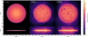 |
Fig. A.1 Projected gas surface density at the end of phase I for all simulations, as well as at t = 0 Myr (initial conditions). |
Before starting the simulation we aim to analyse, our simulated galaxies undergo an initial development phase that we call phase I. During this phase, the galaxies develop from a smooth gaseous density distribution to a turbulent and structured distribution which we start our final simulation from.
We show these start and end points of phase I in Fig. A.1. The left panel depicts the initial smooth density distribution following Equation 6 in a projection along the y and z axis. The following panels show the developed state at the end of phase I of our simulation runs. The general behaviour also observed in Fig. 2 is already prevalent at this time.
Due to numerical limitations in the mesh refinement, during that phase we loose some supernova which explode in regions with strongly diverging gas motion. This applies to 1.8% of all supernova in F3000HD and 6.3% in MW3000HD. During phase II, which is the phase we analyse, this fraction lowers to about 0.6% for both simulations.
Appendix B Resolution study
As a test of convergence we conducted simulations of both potentials also with a mass resolution 1000 M⊙. Overall we see very good agreement with our fiducial runs F3000HD and MW3000HD.
In Fig. B.1 we show the correlation between cell size and cell density, for F1000HD and F3000HD at about 2500 Myr in phase II. It is apparent that in the higher resolution simulation the cells get to lower sizes and correspondingly higher densities due to the lower target mass (up to ∼10−21.4 g cm−3 compared to ∼10−22 g cm−3)
In Fig. B.2 we present the SFR and depletion time τ of the fiducial simulations F3000HD and MW3000HD (same as Fig. 7), overlaid with the curves of F1000HD (orange) and MW1000HD (green). Since running with 1000 M⊙ resolution is more computationally costly, MW1000HD did just run up to about 3000 Myr, i.e. 1000 Myr into phase II. We see excellent agreement between the SFRs produced by F3000HD and F1000HD, as well as between MW3000HD and MW1000HD within the first 1000 Myr of phase II. Correspondingly, the depletion times of the simulations agree as well. At later stages of the simulations, SFR tends to be slightly higher at higher resolution, because of the increased ability of gas to collapse to high density. However, this effect is mild.
The distribution of gas in temperature and density (Fig. B.3, same as Fig. 3, but for MW1000HD and F1000HD) also shows no noticeable difference between 3000 M⊙ and 1000 M⊙ target mass in both potentials. Gas reaches slightly higher densities (as already described) and temperatures with lower target mass, but overall we see good convergence.
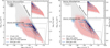 |
Fig. B.1 Volume-density distribution of cells in F3000HD (left) and F1000HD (right) at about 2500 Myr. Contour levels enclose 10%, 30%, 50%, 70% and 90% of cells. |
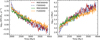 |
Fig. B.2 Star formation rate history (left) and depletion time (right) for F3000HD (blue), MW3000HD (red), F1000HD (orange), and MW1000HD (green). We limit the measurement to ±1 kpc above and below the Galactic plane. We find good agreement in SFR between simulations with 3000 M⊙ and 1000 M⊙ target mass. |
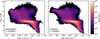 |
Fig. B.3 Temperature-density plot for F1000HD and MW1000HD at the fiducial analysis time of 2500 Myr. We find good agreement with Fig. 3. |
All Tables
All Figures
|
Fig. 1 Gravitational potential and acceleration. Left: non-axisymmetric component of the Milky Way external potential. Right: slices through the centre of the galaxy of the acceleration parallel to the Galactic plane in simulations F3000HD (left column) and MW3000HD (middle column) and their relative difference (right column) at t ≈ 2500 Myr. The first row corresponds to the contribution to the acceleration from the external potential, and the second is the contribution from the self-gravity of the gas and the newly created stars. |
| In the text | |
|
Fig. 2 Surface density of total gas (first column), ionised hydrogen (second column), stars (third column), and the temperature in a slice through the midplane (fourth column) for simulations MW3000HD (first row) and F3000HD (second row) for the inner 15 kpc. |
| In the text | |
|
Fig. 3 Temperature-density plot for the conducted simulations at the fiducial time of 2500 Myr. All phase plots show a three-phase structure of the ISM, with a hot low-density phase and a colder phase extending to higher densities, and the beginning of a cold phase at densities ρ > 10−24 g cm−3. Some mass is also stored in hot higher density gas, probably because of heating by stellar feedback. |
| In the text | |
|
Fig. 4 Volume-weighted density distribution of gas (left) and stars (right) in the radial (upper row) and vertical (lower row, averaged from 8 to 9 kpc) directions for F3000HD (blue) and MW3000HD (red) averaged from 2450 to 2550 Myr. Shaded regions indicate the 16th to 84th percentile. The density distributions generating our adopted external potentials are indicated in grey, dotted for the flat potential and dash-dotted for the Milky Way model. In the radial direction, we took into account mass up to z = ±50 pc. |
| In the text | |
|
Fig. 5 Height of the plane containing 75% of the mass at a given radius for all the simulated mass (left) and the simulated gas and newly formed stars (right) in MW3000HD (red) and F3000HD (blue). In grey, we present height for stars in the Milky Way potential, i.e. the underlying, not explicitly simulated mass distribution. Shaded regions indicate 16th to 84th percentile. In all simulations, stars are more concentrated to the disc plane than gas. |
| In the text | |
|
Fig. 6 Azimuthal profile of the normalised fluctuations of the gas (top), stars (middle), and SFR (bottom) surface densities at t = 2500 Myr. These are compared with the normalised fluctuations of the contributions of the external non-axisymmetric components of the potential, with the bar (green) and the spirals (pink), associated with the right vertical axis of each panel, which is reversed so that lower values are on top. The data have been averaged over a radius range of 1 kpc, and the shaded area represents the radial variations. |
| In the text | |
|
Fig. 7 Star formation rate history (left) and depletion time τ (right) for F3000HD (blue) and MW3000HD (red). We limited the measurement to ±1 kpc around the Galactic plane. Changing the potential does not result in a change of the overall SFR at the fiducial analysis time. |
| In the text | |
|
Fig. 8 Star formation rate surface density in MW3000HD and F3000HD in radial bins for the central (Rgal < 6 kpc) region (two left-hand panels) and whole disc (two right-hand panels). |
| In the text | |
|
Fig. 9 Total mass enclosed in 1.5 kpc, 3 kpc, 4.5 kpc, and 6 kpc normalised by the initial mass within this radius at the beginning of phase II (time t0) for F3000HD (blue) and MW3000HD (red). For MW3000HD we find an increase of about 50% in enclosed mass in the innermost 1.5 kpc. |
| In the text | |
|
Fig. 10 Stellar mass fraction formed in spirals in MW3000HD (top-right panel) and formed stellar mass in the Rgal – Φ-projection for the MW3000HD disc region (6 kpc ≤ Rgal < 20 kpc, top-middle panel) and bar region (Rgal < 6 kpc, top-left panel), corrected for the corresponding pattern rotation, as well as for the disc region of F3000HD, corrected for a pattern speed of Ω = 15.0, 26.0 and 35.0 km s−1 kpc−1 (bottom row). Contour lines indicate 10%, 30%, and 50% of the maximum stellar mass formed (excluding the region of extremely high formed stellar mass at < 0.1 kpc for MW3000HD bar region, upper left). For the MW3000HD disc region, the upper-middle interarm regions are shaded out. |
| In the text | |
|
Fig. 11 Grouped star formation: mass of group (first row), mass fraction of stars born in groups (second row), activity time (third row), and volume of groups (fourth row) for F3000HD (blue) and MW3000HD (red) in the Galactic centre (≤2.5 kpc, left column), inner region (≤5 kpc, middle column), and disc (>5 kpc, right column). Vertical lines indicate median values, which are written out at the upper left or right. Faint lines indicate distributions and medians for a min_cluster_size of three (dashed) and seven (dotted). The corresponding median values are given in brackets. |
| In the text | |
|
Fig. 12 Grouped supernovae: number of association members (top row), fraction of supernova exploding within groups (second row), activity time (third row), and extend of groups (fourth row) for F3000HD and MW3000HD for t = 2450–2550 Myr. Vertical lines indicate median values. Faint lines indicate distributions and medians for a min_cluster_size of 3 (dashed) and 7 (dotted). Corresponding median values are given in brackets. |
| In the text | |
|
Fig. A.1 Projected gas surface density at the end of phase I for all simulations, as well as at t = 0 Myr (initial conditions). |
| In the text | |
|
Fig. B.1 Volume-density distribution of cells in F3000HD (left) and F1000HD (right) at about 2500 Myr. Contour levels enclose 10%, 30%, 50%, 70% and 90% of cells. |
| In the text | |
|
Fig. B.2 Star formation rate history (left) and depletion time (right) for F3000HD (blue), MW3000HD (red), F1000HD (orange), and MW1000HD (green). We limit the measurement to ±1 kpc above and below the Galactic plane. We find good agreement in SFR between simulations with 3000 M⊙ and 1000 M⊙ target mass. |
| In the text | |
|
Fig. B.3 Temperature-density plot for F1000HD and MW1000HD at the fiducial analysis time of 2500 Myr. We find good agreement with Fig. 3. |
| In the text | |
Current usage metrics show cumulative count of Article Views (full-text article views including HTML views, PDF and ePub downloads, according to the available data) and Abstracts Views on Vision4Press platform.
Data correspond to usage on the plateform after 2015. The current usage metrics is available 48-96 hours after online publication and is updated daily on week days.
Initial download of the metrics may take a while.