| Issue |
A&A
Volume 704, December 2025
|
|
|---|---|---|
| Article Number | A348 | |
| Number of page(s) | 15 | |
| Section | Astrophysical processes | |
| DOI | https://doi.org/10.1051/0004-6361/202452612 | |
| Published online | 22 December 2025 | |
Disk evolution and black hole mass constraints on EXO 1846−031 based on NICER/XTI, Insight-HXMT and NuSTAR observations
1
Department of Astronomy, School of Physics and Astronomy, Yunnan University, Kunming, Yunnan 650500, China
2
RIKEN, 2-1 Hirosawa, Wako, Saitama 351-0198, Japan
3
Department of Physics, Tokyo Institute of Technology, 2-12-1, Ookayama, Tokyo 152-8551, Japan
4
Department of Physics, Ehime University, 2-5, Bunkyocho, Matsuyama 790-8577, Japan
5
Key Laboratory of Particle Astrophysics, Institute of High Energy Physics, Chinese Academy of Sciences, Beijing 100049, China
6
Dongguan Neutron Science Center, Zhongziyuan Road, Dongguan 523808, People’s Republic of China
7
University of Chinese Academy of Sciences, Chinese Academy of Sciences, Beijing 100049, China
★ Corresponding author: This email address is being protected from spambots. You need JavaScript enabled to view it.
Received:
15
October
2024
Accepted:
28
September
2025
Abstract
We studied the spectral properties and the accretion disk evolution of the black hole candidate EXO 1846−031, based on NICER/XTI observations. The combined models, consisting of a multicolor disk and a Comptonized component, revealed a truncated disk at the beginning of its 2019 outburst. To obtain better constraints on system parameters (i.e., inclination and mass), we further investigated the reflection features using simultaneous NICER and NuSTAR observations. In combination with the analysis of HXMT reflection spectra, a lower inclination (i.e., i < 55°) is preferred based on the reflection model fittings. We also studied the MAXI and Swift/XRT data during the transition toward the low-hard state in the end of the outburst as a complement to NICER data. Using the Swift/XRT transition flux and the latest empirical Eddington ratio at the index transition toward the low-hard state, the model-independent black hole mass was estimated to be M < 8.2 M⊙ given a distance of 2.4 − 7.5 kpc. In addition, we discuss the mass constraints assuming different models and different inclinations and spins. Assuming an extreme spin (a = 0.998) and adopting a complex model consisting of a relativistic disk and a reflection component to the HXMT spectra in the high-soft state, a black hole mass of  at a source distance of 7 kpc is suggested.
Key words: accretion, accretion disks / black hole physics / stars: black holes
© The Authors 2025
 Open Access article, published by EDP Sciences, under the terms of the Creative Commons Attribution License (https://creativecommons.org/licenses/by/4.0), which permits unrestricted use, distribution, and reproduction in any medium, provided the original work is properly cited.
This article is published in open access under the Subscribe to Open model. This email address is being protected from spambots. You need JavaScript enabled to view it. to support open access publication.
1. Introduction
Accretion onto a compact object is widely accepted to be the engine driving its outburst or burst (when the X-ray flux increases orders of magnitude compared with the quiescent phase) in X-ray binaries (e.g., Lewin et al. 1995). At accretion rates in excess of a few percent of the Eddington rate, most black hole binaries (BHBs) are found in the so-called high-soft state, whose X-ray spectrum is dominated by a soft component and is well described by the standard thin disk model with a typical temperature of < 2 keV (Shakura & Sunyaev 1973). While a “low-hard” state is found at lower accretion rates when the X-ray spectrum is dominated instead by a nonthermal component and usually can be described by a hard power law. The mechanism how accretion works in the evolution of spectral states in BHB outbursts is not fully understood. Therefore investigations of the radiation processes in each state and their evolution with the mass accretion rate by studying the X-ray spectral continuum are important for achieving a better understanding of accretion physics.
The continuum fitting can be used to provide the information of black hole spin, employing a relativistic accretion disk model (Li et al. 2005). Apart from the thermal and non-thermal components found in spectral continuum, emission-line features have been widely observed in BHBs (see e.g., Miller 2007; García et al. 2015). In particular, the broad emission line centered at 6.4 − 7 keV as the most prominent feature of disk reflection, is important for spin measurements. Reflection spectroscopy is frequently used to characterize the features of a fluorescent Fe-Kα emission between 6.4 and 7 keV and a Compton hump in the hard band (20–50 keV). The broad emission line feature is thought to be produced when the nonthermal emission illuminates the accretion disk (see, e.g, Lightman & White 1988; George & Fabian 1991). Recently in the BHB XTE J1550−564, the disk reflection in the very soft state was found to be produced by self-irradiation of the innermost part of the accretion disk (Connors et al. 2020). Both of the above methods infer the value of spin indirectly by measuring the inner radius of the accretion disk and both of them also provide the geometrical parameter of the system: the inclination. In general, precise measurements of spin are complicated, and can often be model-dependent, due to our limit knowledge of the system parameters and geometry.
EXO 1846−031 has been proposed to be a black hole candidate based on the ultra-soft component in the spectra of its 1985 outburst (Parmar et al. 1993). This source was detected in outburst in 2019 July 23 by MAXI/GSC (Negoro et al. 2019), following a long quiescent period since it was first discovered in 1985 April 3. (Parmar & White 1985). Follow-up observations were performed in multi-wavelength bands by multiple instruments, supporting various investigations of this source, despite some inconsistencies were found among them. Type-C QPOs were found in NICER (Bult et al. 2019) and Insight-HXMT (Liu et al. 2021) observations. Draghis et al. (2020) analyzed the reflection features in NuSTAR spectra in the beginning of the outburst and suggested a nearly maximal spin and high inclination of 73° for EXO 1846−031. Wang et al. (2021) argued for a comparatively lower inclination of ∼40° and suggested the presence of an ionized disk wind with velocities up to 0.06c based on studies of the Insight-HXMT and NuSTAR data. Ren et al. (2022) reported the detailed HXMT energy spectra analysis and suggested a decreasing harding factor from the low-hard state to the high-soft state. A distance range of 2.4 − 7.5 kpc and a jet speed of βint = 0.29c were revealed from radio observations (Williams et al. 2022). Nath et al. (2024) investigated the evolution of spectra and the properties of accretion flow by adopting the two component advective flow (TCAF) model to the combined spectra of multiple satellite instruments.
Figure 1 shows the X-ray light curves together with the hardness ratios of EXO 1846 − 031 with NICER, Swift/XRT and MAXI observations during its 2019 outburst. Although, the Swift/XRT data exhibit comparatively larger hardness ratio values, the hardness ratios among NICER, SWIFT/XRT and MAXI reveal the similar variation trends, which reveal the decreasing tendency before MJD 58880 and an increasing tendency after MJD 58900, suggesting the state transitions from the hard to the soft and back toward the hard during the outburst.
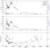 |
Fig. 1. Light curves and hardness ratios of EXO 1846−031 during its 2019 outburst as functions of MJD. Top panel shows the light curves in the soft bands: 0.3 − 4 keV for NICER/XTI and Swift/XRT; 2 − 4 keV for MAXI/GSC. Middle panel shows the light curves in hard bands: 4 − 6 keV for NICER/XTI, 4 − 10 keV for Swift/XRT and MAXI/GSC. Bottom panel shows the corresponding hardness ratio for NICER/XTI (4 − 6 keV/0.3 − 4 keV), Swift/XRT (4 − 10 keV/0.3 − 4 keV), and MAXI/GSC (4 − 10 keV/2 − 4 keV), respectively. The NICER (black circles) and Swift data (open circles) are depicted on the left y-axis, and the MAXI data (blue triangles) are depicted on the right y-axis. The green and red bars represent the times of the NuSTAR and HXMT observations. |
In this work, we study the spectral properties and disk evolution of EXO 1846−031 during its 2019 outburst using NICER/XTI data with models consisting of a multicolor disk and a nonthermal component. We reexamine the reflection features in HXMT spectra and the reflection features in the increasing phase using NICER and NuSTAR spectra. We further investigate the reflection features in the high-soft state using NICER and NuSTAR spectra, and we ascertain the inclination, which had been found to be divergent in previous studies. Finally, we discuss the mass constraints of the central object obtained exploiting different methods.
2. Observations and data reduction
2.1. NICER observations
We employed all the NICER observations available from the HEASARC archive1during the 2019 outburst of EXO 1846−03. We reduced the data with level 2 calibration using the NICER software, nicerl2. The NICER spectra and light curves are built using nicerl3-spect and nicerl3-lc with the calibration file (CALDB xti20221001). Each NICER spectrum was extracted from one observation ID and the background spectrum for each observation is built by nibackgen3C502. The adjacent energy bins for each spectrum were grouped until they satisfied a 60 photon count threshold. The spectra from observation ID: 3200760103 and ID: 3200760104 were excluded from this study, as their number of spectral bins was less than 40 after the rebinning.
2.2. NuSTAR observations
NuSTAR performed six observations for EXO 1846 − 031, and we employed three of those observations (ID: 90501334002, ID: 80502303004 and ID: 8050230300) to create simultaneous spectra adjacent to NICER observations. We extracted the NuSTAR spectra of the source and background using the NuSTAR Data Analysis Software (NuSTARDS v2.0.0) with two circular regions of 150″(one centered at the source and another centered away from source). For ID 90501334002, we extracted the spectrum setting the time period the same as that of the NICER observation (ID: 2200760104) since the shape of spectrum continuum changed significantly during this NuSTAR observation time. The detailed comparisons of spectral shape are shown in Section 3.2. For observation ID 80502303004 and ID 80502303008, we extracted one spectrum per observation. Prior to fitting the spectra in XSPEC, we combined the adjacent energy bins until they satisfied a 30 photon counts threshold for ID 90501334002. We then grouped the data with a minimum signal-to-noise ratio (S/N) of 5 for ID 80502303004 and ID 80502303008 when the NuSTAR X-ray luminosity decreased. Grouping the data with a minimum S/N of 5 for ID 90501334002 results in negligible differences in spectral fittings.
2.3. HXMT observations
Over the broad energy range of 1 to 250 keV with low-energy, medium-energy, and high-energy detectors, HXMT also performed point observations for EXO 1846 − 031 during its 2019 outburst (Zhang et al. 2020). We used the data from observation ID: P021405002, which has the longest exposure time, to study the reflection radiation with good statistic. The HXMT spectra of source and background were extracted following the official guide3 and using the software HXMTDAS with CALDB version 2.06. The criteria for screening are the default values in the HXMT pipeline software: hpipeline. The spectra in this observation were merged when they are from the same detector. A 100 photon count threshold was applied to HXMT spectra prior to the spectral analysis.
3. Results and analysis
In this study, we analyzed time-averaged energy spectra using XSPEC 12.13.0. The errors are quoted at the statistical 90% confidence limits for a single parameter using the XSPEC error function.
3.1. NICER/XTI spectral fittings and the accretion disk evolution
We fit NICER/XTI spectra (56 in total) in the energy range of 1.3 − 10 keV with: (1) a combined model consisting of a multicolor disk (diskbb in XSPEC; Mitsuda et al. (1984)) and a power-law component representing the hard tail; (2) a convolved model consisting of a diskbb model modified with Comptonization (simpl in XSPEC; Steiner et al. (2009)); (3) a combined model consisting of a diskbb and a thermally Comptonized continuum (Nthcomp in XSPEC; Życki et al. 1999) representing the hard tail. We used only a diskbb or a simple power-law/Nthcomp model when including a nonthermal or a thermal component will not significantly improve the goodness of fit (Δχ2 < 0.02).
For the combined model, diskbb+Nthcomp, we fixed the electron temperature (kTe) at 60 keV and allowed the seed photon temperature (kTbb) to remain the same as the innermost disk temperature (Tin). Changing electron temperature from 30 keV to 300 keV resulted in negligible differences in other parameters. We set the redshift to be 0 when fitting the spectra.
To account for the interstellar absorption, we multiplied the TBabs model to the above models, employing the abundance table by Wilms et al. (2000). The hydrogen column density NH was fixed to 6.1 × 1022 cm−2, which is the averaged NH value in the high-soft state when the disk component is dominant. From MJD 59724, the photon index was fixed to 2.0 since the nonthermal component was too weak to constrain the photon index well. Fixing the photon index results in a negligible influence on the parameters in the other model components.
We note that there is a feature in the 1.7 − 2.4 keV range that could be explained by the Silicon absorption edge (∼1.84 keV)4. Therefore, we additionally added a convolved model edge to the above four baseline models to improve the fittings. A Gaussian is added to the baseline models when the iron line feature (∼6.4 keV) was obviously observed in bright phases. Nath et al. (2024) employed a similar operation for those two features when fitting NICER spectra. For the spectra that did not show obvious features in ∼1.8 keV and/or ∼6.4 keV due to the statistic limit, the edge and/or gauss component was omitted. Figure 2 shows the example of NICER spectrum and the comparisons of fit goodness when including edge and gauss components, respectively. There could be reflection feature above 5 keV in NICER spectra; however, the main goal of analyzing NICER spectra in this section is to understand the evolution of X-ray state and the evolution of the accretion disk. A detailed study of the reflection irradiation was carried out using the NuSTAR and HXMT observations, as explained in the following sections.
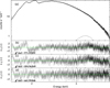 |
Fig. 2. Panel (a) shows the NICER spectrum (ID 2200760101) fitted with TBabs*(simpl*diskbb+gauss)*edge. The dotted line represent the Gaussian component. Panel (b) shows the residuals in terms of sigma for the model, TBabs*(simpl*diskbb). Panel (c) shows the residuals for the model, TBabs*(simpl*diskbb)*edge. Panel (d) gives the best-fit model, TBabs*(simpl*diskbb+gauss)*edge. |
Figure 3 shows the evolutions of NICER spectral parameters. We observed the deviations of the trends of parameters among different models from MJD 58700 to MJD 58725. During this period, the complex model diskbb+power-law shows a comparatively high inner disk temperature (Tin) and a smaller disk normalization. The diskbb+NthComp model and the simpl×diskbb model reveal similar trends in terms of Tin and the photon index; however, the diskbb+NthComp model gives a small disk normalization as the diskbb+power-law model does. We also note that the disk component was found to be unnecessary in several observations for diskbb+NthComp model, suggesting a comparatively stronger nonthermal component that could be described by a large corona covering the accretion disk. The disappearance of the disk was also found in one observation around MJD 58700 (ID:2200760105) for the diskbb+power-law model. It is not common to find the accretion disk to have disappeared after being found at the beginning of an outburst and when Tin has started to increase. The variation trends converged to the similar values after MJD 58725 for the three complex models. The nonthermal component was not required for three observations, marked as black points in Figure 3. Although the models resolve different trends of spectral parameters between MJD 58700 to MJD 58725, the overall evolutions of the disk temperature, photon index, and disk normalization, are consistent with the typical patterns of the state evolution from the low-hard to the high-soft and back to the low-hard for a BHB outburst.
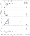 |
Fig. 3. Evolution of fitting parameters of NICER spectra during the 2019 outburst of EXO 1846 − 031. From top to bottom, each panel shows the innermost disk temperature, the normalization of disk, the photon index, and the reduced χ2, respectively. The arrows in the top panel point the simultaneous NuSTAR observations and the dashed arrow points the date of HXMT observation used in this study. |
To clearly depict the evolution of accretion disk, as shown in Figure 4, we estimated the innermost disk radius (rin) using Equation (1) and assuming an inclination of 40 degree (Wang et al. 2021) and a source distance of 7 kpc (Williams et al. 2022).
 |
Fig. 4. Evolution paths of the innermost disk radii. The blue crosses represent the rin estimated from the fitting results with diskbb+NthComp model and the black crosses represent the rin corrected using Equation (1). |
In Figure 4 we also show the rin values after accounting for the scattered photons, assuming the Comptonized component is purely originated from the disk photons. This modified rin of diskbb+NthComp model in the intermediate state is more consistent with the values given by simpl×diskbb model. We also note that the small rin derived by diskbb+power-law model in the intermediate state is unphysical, given the latter constant values are considered to be the radius of the inner stable circular orbit (ISCO). These results indicate that the derived disk radii in the spectra whose nonthermal components are comparatively strong and a power-law or downwardly curving continuum (soft deficit) at low energies suggests an inner disk radius that is much smaller than that derived from an upwardly curving (soft excess) continuum. From this point of view, a realistic Comptonization model (but not an empirical model such as a power-law model) would better reflect the actual physical properties of the inner disk region when there is a strong contribution from the Comptonization component. The evolution of a truncated disk extending toward the ISCO can be inferred according to the rin values derived from simpl×diskbb models and diskbb+NthComp model after accounting for the scattered photons. On the other hand, the rin directly estimated from the shape of spectral continuum was thought to be an “apparent” innermost radius (Kubota et al. 1998), a more “realistic” radius, Rin, should account the effects of boundary conditions and be corrected as Rin = ξκ2rin. Here, the κ is the color-temperature correction (the ratio of color temperature to effective temperature) with a typical value of 1.7 − 2.0 (Shimura & Takahara 1995) and the ξ is the correction factor for the boundary condition with a typical value of 0.412 (Kubota et al. 1998). Changes in the surface properties of the accretion disk (rather than the appearance or disappearance of the entire inner regions) can also lead to the dramatic changes in disk spectrum and, therefore, a stable inner radius at ISCO existing during the whole course of the outburst (rather than a truncation model) has often been discussed in previous studies (Merloni et al. 2000; Reis et al. 2010). Ren et al. (2022) indicated that their unexpected smaller inner radii derived from HXMT spectral fittings in the low-hard and intermediate states can be modified by a comparatively larger κ to make them comparable with ISCO. Within the limited information of this source, the detailed analysis of boundary conditions is beyond our current work and, thus, the realistic disk evolution between MJD 58700 and MJD 58720 is reserved for in-depth analysis in future. Nevertheless, our fitting results strongly suggest a truncated disk prior to MJD 58700.
Nevertheless, the constant innermost disk radius in the high-soft state (in other words, the ISCO) shows negligible differences using different models to represent the nonthermal component. Our estimated rin of ∼30 km, is comparable to the rin of ∼27 km derived from HXMT spectral fittings in the high-soft state (Ren et al. 2022) assuming an inclination of 40 degree and a source distance of 7 kpc. In this study we employed the averaged inner radius derived from simpl×diskbb model as the ISCO after applying a color-temperature correction of 1.7 and a boundary correction of 0.412 to the estimated rin. The ISCO is estimated to be 36.3 ± 4.2 km assuming an inclination of 40 degree and a source distance of 7 kpc. This can be expressed as
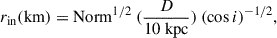 (1)
(1)
where D is the distance and i is the inclination angle (Mitsuda et al. 1984; Makishima et al. 1986).
3.2. NuSTAR and HXMT spectral fittings
We fit three simultaneous NICER and NuSTAR observations, along with one HXMT observation using reflection models. The observations are listed in Table 1. For each joint NICER-NuSTAR spectrum, the model fitting was adopted in 1.3 − 10 keV of NICER and 4 − 79 keV of NuSTAR. For the HXMT spectrum, the model fitting was adopted in the 2 − 9 keV of LE instrument and 9 − 20 keV of HE instrument. When performing a joint fitting of NICER (ID 2200760104) and NuSTAR (ID 90501334002) spectra at MJD 58698.1, we note that the NuSTAR observation is longer than the NICER observation and that the spectrum continuum are different in 5 − 10 keV between the two observations. Considering that the spectral shape can change dramatically in the phase closest to the transition from low-hard state to the intermediate state, we extracted the NuSTAR spectrum having exactly the same observation time as that of NICER and found that this extracted NuSTAR spectrum and NICER spectrum are consistent in 5 − 10 keV. Figure 5 shows the comparisons between this NICER and NuSTAR spectra, fitted with a diskbb+power-law model to show the differences of spectral continuum. Here, we fixed the disk parameters and photon index to the best-fit values obtained form NICER spectral fittings (detailed in Section 3.1).
NICER, NuSTAR and HXMT observations of EXO 1846−031 used in reflection model fittings.
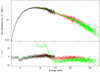 |
Fig. 5. Simultaneous NuSTAR/FPMA and NICER/XTI spectra at MJD 58698.1 fitted with a complex model of constant*TBabs*(diskbb+power-law). The black data points represent the NICER/XTI (1.3–10 keV) spectrum with observation ID 2200760104. The green data points represent the NuSTAR/FPMA spectrum (4–79 keV) with the observation ID 90501334002. The red data points represent the NuSTAR/FPMA spectrum with the same NuSTAR observation ID as that of green points but having the exactly same observation period as that of NICER spectrum. |
The strong reflection features make this source an ideal target to test the reflection group models. Based on Wang et al. (2021), we employed the relxillNS model (García et al. 2022) in the high-soft state, as a comparison to the frequently employed relxill model (García et al. 2014). Utilizing the relxillNS to describe a reflection spectrum that could possibly be produced by the disk self-irradiation in a very soft state for BHBs was first reported in the work of Connors et al. (2020). The relxillNS was originally designed for the reflection originating from the accretion disk in a neutron star system, where the illuminating source is a single-temperature blackbody. In this work, we use it as an approximate approach to describe the reflection spectra in the soft state when nonthermal component below 20 keV is modest. As in Connors et al. (2020) and Wang et al. (2021), we assumed the inner disk temperature at ISCO to be sufficient to illuminate the disk.
We adopted two reflection models (relxill and relxillNS) to the spectral fittings and we employed a diskbb or a relativistic accretion disk (kerrbb in XSPEC; Li et al. (2005)) to represent the disk emission. A cutoff power-law model was correspondingly used to represent the nonthermal component if the relxill was adopted and a NthComp model was correspondingly used if the relxillNS model was adopted. The absorption model TBabs was added to the baseline model with NH fixed to 6.1 × 1022 cm−2. The convolved model edge was also added to the baseline models when fitting the joint NICER-NuSTAR spectra to improve the fittings in ∼1.8 keV (see Section 3.1), where the threshold energy was fixed to 1.84 keV. To avoid the mismatch between NICER and NuSTAR possibly caused by cross calibration, the NuSTAR data below 4 keV were ignored. When fitting the joint NICER+NuSTAR spectra, the constant factor of FPMB was fix to unity, the factor of NICER constN was set to vary in 0.9 − 1.1, and the factor of FPMA constA was set to vary in 0.95 − 1.05. When fitting HXMT spectra, the constant factor of ME was fixed to unity, and the factor of LE constLE was set to vary in 0.9 − 1.1.
For the reflection models, we fixed the emissivity index q1 = q2 = 3, and we fixed the outer disk radius to 400 gravitational radii, redshift at zero, and the reflection fraction at –1. The reflection fraction is defined in the frame of the primary source as ratio of intensity emitted toward the disk compared to escaping to infinity. Setting it to a negative value makes reflection models only account for the reflection component. We let the ionization of the disk Log(ξ) vary from 0 to 4.3 and the iron abundance, AFe, varies in the range of 0.5 − 6.0 (Wang et al. 2021). The photon index and Ecut were linked between the relxill model and cutoff power-law model. The electron temperature kTe was linked between the relxillNS model and NthComp model. The Ecut/kTe was set to vary from 30 to 300 keV. The seed photon temperature was linked between relxillNS model and NthComp model, and was also linked to the disk temperature, Tin, if a diskbb model was used. We fixed the inner radius Rin at the ISCO when fitting the spectra in the high-soft state.
For the kerrbb model, we fixed the ratio of η (the ratio of the disk power produced by a torque at the disk inner boundary to the disk power arising from accretion) at zero and source distance at a typical value of 7 kpc. We linked the inclination and spin to the reflection model. We allowed the black hole mass and the mass accretion rate to vary, keeping the other parameters of kerrbb at their default values (i.e., the spectral hardening factor was fixed at 1.7, rflag at 1.0, and lflag at 0). The black hole mass was limited to 1 − 30 M⊙, a typical mass range of observed Galactic black hole transients. We note that the observation only gives a modified disk emission (or a modified inner disk radius) with a spectral hardening factor, fcol. The kerrbb model determines spin assuming the actual inner disk radius as the inner stable circular orbit and the inner stable circular orbit is a monotonic function of spin. Therefore, an independent estimate, fcol, is needed in order to estimate spin. Provided that inclination and distance are known to sufficient accuracy, a larger fcol results in a smaller spin with kerrbb model but the decreasing slope varies among the observations (see e.g., Shafee et al. 2006). Investigating the comprehensive impact of fcol for a complex model consisting of kerrbb and the reflection component is beyond our current studies.
Table E.1 lists the fitting parameters of the combined models of diskbb and reflection models for the four observations, X1, X2, X3, and X4. Table E.2 lists the results of the combined models of kerrbb and reflection models. Figure 6 shows the reflection model fittings using X1 as an example. The comparisons of the reflection models for X2, X3 and X4 and their spectral shapes can be found in Fig. A.1 and Fig. B.1 in the appendix.
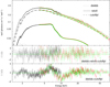 |
Fig. 6. Joint NICER+NuSTAR spectrum fitted with the diskbb+relxill+cutoff power-law model for X1 observation, where the NICER data is marked in black, NuSTAR/FPMA is marked in red and NuSTAR/FPMB is marked in green. The disk component is represented by dotted line, the nonthermal component is represented by dashed line and the reflection model is represented by solid line. The goodness of fit with diskbb+cutoffpl model is shown in the bottom panel for compassion. The bins in the figure are plotted that have at least 50 sigma, or are grouped in sets of five bins, to make the goodness of fit easier to compare. |
4. Discussions
4.1. Model fit comparisons
To quantitively compare the performance of models, we employed the χ2 statistics through the standard χr2 = χ2/d.o.f., where dof is the degree of freedom, and we introduced the Akaike information criterion (AIC). The AIC technique does not reply on likelihood ratio testing neither require the compared model to be nested (Petrov & Csáki 1973). We adopted the Equation (5) in (Emmanoulopoulos et al. 2016) to calculate the AICc,
 (2)
(2)
where CL is the constant likelihood of the true hypothetical model, k is the number of free model parameters, and N is the number of data points. The difference between two models, Δ[AICc]=AICc, 2 − AICc, 1, will effectively cancel out the constant term CL and can be used to compare the model fits, referring a general rule: a Δ[AICc] value smaller than 2 suggests that both models fit the data at least equally well, Δ[AICc] values between 3 and 7 indicate that the model 2 has considerably less support; whereas if Δ[AICc]> 10, then the model 2 is highly unlikely (Burnham & Anderson 2002). As CL should be the same for the same observation data and only the difference in terms of AIC matters in the model comparison; in Table E.1 and Table E.2, we list the AICc assuming CL is 0.
To make the comparison easier to follow up on, we first discuss the model fits for the group of the combined models of diskbb+reflection. Then we did the same for the group of the combined models of kerrbb+reflection. Finally we conduct overview comparisons of the two groups of models, as described below.
(1) diskbb+reflection models:
For the same model and the same observation, we found that the Δχr2 < 0.02 when the spin is fixed to the maximum 0.998 and is set to free, while the spin value can down to the minimum –0.998 when the spin is free for observation X2 and X4 with a 90% confidence level. This suggests that the spin is difficult to constrain using diskbb+reflection models.
For the different reflection models relxill and relxillNS, we used the Δ[AICc] to evaluate the model preference. For X1 the relxillNS model is not able to fit the spectrum well (χr2 > 2) and, thus these results are not listed in Table E.1. For X2, the Δ[AICc] is much larger than 10 regardless of whether the spin is fixed or varying, indicating that the relxillNS model is unlikely to be preferred. The relxillNS model is less supported according to the Δ[AICc] of X4, although the difference of AIC is comparatively smaller. For X3, obtained by a different instrument HXMT, the AIC values reveal that relxill is unlikely preferred. A evolution of the seed spectrum of the reflection component from the cutoff power-law to the black body and eventually toward back to the cutoff power law is suggested.
(2) kerrbb+reflection models:
For observation X1, the relxillNS model cannot fit the spectrum well (χr2 > 2) and, thus it is not listed in Table E.2. For X2, X3 and X4, the relxillNS model is preferred, considering its χ2 is smaller and the AICc of the relxill model is larger than that of the relxillNS model.
For the same observations of X2 and X4, a retrograde spin is suggested by the comparatively smaller AIC values. The retrograde spin is consistent with the result when fitting a NICER spectrum whose disk component is merely dominant (e.g., ID: 2200760143) with a kerrbb model, possibly due to the dominance of the soft X-ray emissions in NICER spectra.
The χ2 values of kerrbb+relxillNS model are identical for the same observation, no matter whether the spin was set to the maximum 0.998 or set to be variable. Although, statically, the AIC manifests a modest ascendancy in lower spin with kerrbb+relxillNS model, the small black hole masses suggested by X2 and X4, lead to a result of 29%LEdd and 31%LEdd given a source distance of 7 kpc, where LEdd is the Eddington luminosity. These Eddington ratios are close to or exceed the threshold (L/LEdd ≤ 0.3) that the disk obeys ISCO suggested by numerical simulations (see, e.g., Fragile et al. 2018), lending less support to the lower mass cases. In addition, a transition to the very high state is supposed to occur at 20%−100%LEdd (Kubota & Makishima 2004), which is not found in this outburst. This also suggests the lower mass case (the retrograde case) is unlikely. The fitting results of X3 are convergent to support a prograde black hole.
(3) Overview of the reflection models:
In looking at the two tables, we can see that if we arbitrarily compare two models for the same observation, the AICc differences are almost at the same order, no matter the spin was fixed to the maximum or set to be free. A retrograde spin case is more unlikely, based on the discussion in point (2). To make the comparisons more concise, we only discuss cases where the spin was fixed to 0.998.
For the X1 observation, the Δ[AICc] between kerrbb+relxill model and diskbb+relxill model is ∼5, suggesting that the kerrbb+relxill model is less supported. The lower preference with respect to kerrbb+relxill model for X1 could be a result of a conflict between a truncated disk, revealved by the NICER spectral fittings in Section 3.1 and the intrinsic assumption of kerrbb model where rin = RISCO. For X2, X3, and X4, the kerrbb+relxillNS model is most likely to be the true model according to the small AICc values. We also note that, in contrast, the kerrbb+relxill show the worst performance for X2, X3, and X4. The Δ[AICc] values between the best fit models in diskbb group and those in kerrbb group for the three observations are ∼10, close to the threshold determining the diskbb group models are unlikely supported.
Besides the preferences purely suggested by the statistic criteria, the physical properties behind models play core roles to determine the proper model. Tying the spin parameter across kerrbb and reflection model has the advantage of reducing the degeneracy of the models. It is widely believed that the appearance of disks around rapidly rotating holes will be substantially different from that of disks around slowly rotating holes; or in other words, they would be different from the standard disk described by the diskbb model. The results from models consisting of a relativistic accretion disk and reflection component are therefore thought be more credible. On the other hand, we note an unexpected large reflection flux when adopting kerrbb+relxillNS to X2 and X4 (see Figure C.1 in Appendix). Numerical simulations suggest a returning radiation in the inner disk exceeding or comparable to that generated locally for extremely high spin case, but the difference of the total disk flux after including the returning radiation will not be significant (∼10%) (Cunningham 1976). Therefore, the validity of the kerrbb+relxillNS fittings for X2 and X4 is challenged, although this model is seen as the best fit based on the statistics. Since the kerrbb+relxill does not have a better goodness of fit either, determining the origin of reflection component can be complex (e.g., the combination of disk and nonthermal component) when the source leaves the intermediate state shortly before (for X2) and the source tends to leave the high-soft state (for X4). The fitting results of kerrbb+relxillNS model for X3 is considered to be the most trusted case from the overview of model comparisons.
(4) Possible absorption and emission component in the broad spectra:
An absorption line at ∼7 keV in NuSTAR spectra at MJD 58698 has been reported by both Draghis et al. (2020) and Wang et al. (2021), presumably originating from the disk wind. For spectra X1 at MJD 58698, introducing the absorption component to the reflection model fittings (as described in Section 3.2) results in negligible effects on other parameters. No obvious absorption feature was found in X2, X3, and X4. To further examine the existence of absorption feature in X1, we tested the spectral fitting by introducing a gabs model representing the absorption component to the diskbb+relxill model, where the spin was fixed to the maximum, the inclination was fixed to 70 degree (Draghis et al. 2020), qin was set to vary in the range of 3 − 10, and qout was set to vary in the range of 0 − 3. The fit slightly improved by Δχ2 = 6.3 for three fewer degrees of freedom (d.o.f.), suggesting the absorption feature is subtle. A narrow emission line at ∼6.7 keV in HXMT spectra, possibly originating from a “transparent” disk wind, was discussed by Wang et al. (2021). To check whether the possible emission feature would contribute to the corrections of reflection model fittings, we added a Gaussian to the models for X3. The spin parameter was fixed to 0.998 as the overall model is too complex to be constrained if spin was variable. The width of the Gaussian is difficult to constrain when it was introduced in diskbb+reflection models. The diskbb+relxill model obtained a slightly better fit with Δχ2/d.o.f. ∼ 0.02 after introduced the emission component. The strength is comparable to that found in Wang et al. (2021), while a lower inclination i < 14.4° has also been suggested. The emission component is less significant when it was added to diskbb+relxillNS model, resulting in a Δχ2/d.o.f. < 0.01 improvement. In diskbb+relxillNS+gauss model, the strength of Gaussian was pegged at 2.6 × 10⁻⁴, with a 90% confidence level and the inclination was limited to i < 29.1°, which is a less significant result than that obtained by Wang et al. (2021). A more obvious emission line appeared with the kerrbb+relxill model. We list the fitting results with the kerrbb+reflection+gauss models for X3 in Table 2 and show their spectra in the appendix (see Figure D.1) for reference. We also attempted to examine the existence of possible narrow emission line in X4. For X4, it is hard to separate the contributions from reflection and that coming from narrow emission line, only the kerrbb+relxillNS+gauss model reveals a narrow emission component comparable to that found in X3 but with less significance. Including this narrow emission line can reduce the unexpected large reflection flux mentioned in part (3), suggesting an inclination of  degree and a black hole mass of
  . X4 fitted with kerrbb+relxillNS+gauss model is shown in Figure D.1 in the appendix for reference.
Fitting results for X3 with Kerrbb+reflection+gauss model.
Overall, introducing an emission component is likely to indicate a lower inclination. Examining the precise feature and significance of the possible emission line as well as its origin requires higher spectral resolution, which is beyond the scope of our current work.
4.2. Inclination
From Table E.1 and Table E.2, we found that most of the reflection model fittings reveal an inclination < 60°, even though there are models showing degenerate spins in one fitting and the best-fit spin can vary significantly from one observation to another. A tighter inclination constraint of 26° −52° can be obtained when assuming a maximum spinning black hole and referring the statistically best-fit models (smallest AIC) for each observation. This inclination range is much lower than the inclination of ∼75° Miller et al. (2019) and ∼73° obtained in Draghis et al. (2020). The Draghis et al. (2020)’s parameters of diskbb+relxill cannot fit the X1 spectra well. The difference could be due to the soft component (of < 3 keV) in the NICER data, and/or the change of spectral shape during the NuSTAR observation (ID: 90501334002) mentioned in Section 3.2. Our inclination is more consistent with the values suggested by Wang et al. (2021). In the work of Wang et al. (2021), they divided the NuSTAR observation into two segments according to the different X-ray flux levels, respectively. Although their reason for dividing the NuSTAR observation is different from ours, the time period of their first segment is similar to the one we set when extracting the NuSTAR spectra and it resulted in a similar inclination. Comparing the reflection models that we used and those in previous papers, we find that the divergent inclination might be caused by the assumption of accretion disk, particularly with respect to the emissivity. A high emissivity index of inner disk region and a quite low emissivity index of outer disk region appear in Draghis et al. (2020), while the linked inner and outer emissivity index qin = qout were used in Wang et al. (2021) and our work. We then checked the possible inclination range with diskbb+relxill model assuming 3 ≤ qin ≤ 10, 0 < qout ≤ 3, Rin = RISCO, a = 0.998, a break radius rg < Rbr < 400rg and the settings (variable ranges) of other parameters (as Section 3.2). The inclination can increase up to 74° with a χ2/d.o.f. = 2134.70/2111 for X1, suggesting a best-fit inclination at 65°. The best-fit inclination is consistent with the inclination of updated by Draghis et al. (2023) using six NuSTAR observations. However, this high inclination requires an extremely low qout in our fitting, which is physically less plausible. Limiting the 1 < qout ≤ 3 will result in an inclination up to 36° with a χ2/d.o.f. = 2134.75/2111. The inclination can increase to 59° and 75° for X2, X4 with χ2/d.o.f. = 1497.29/1640 and 1372.65/1502, respectively (1 < qout ≤ 3, qout is close to the lower limit 1); however, the lower inclination of 50° −55° shows an almost identical performance in fittings (Δχ2/d.o.f. ≤ 0.01). For the HXMT observation X3, the inclination is still well constrained to be 39° −44° with a χ2/d.o.f. = 1133.8/1001 (0 < qout ≤ 3), which is consistent with the result in Table E.1. At the current stage, without any information on the emissivity of the actual accretion disk, a more condensed inclination constraint is hard to obtain. Nevertheless, the inclination was confirmed to be < 55° when employing a Kerr accretion disk to replace the diskbb (kerrbb+relxill as the best-fit model for X1 and X2; kerrbb+relxillNS as the best-fit model for X3, and X4), even when we vary qin (3 − 10) and qout (0 − 3). In the cases of variable qin and qout, the best-fit models containing a Kerr accretion disk display a better (for X3 and X4) or almost identical (for X1 and X2) goodness of fit compared with the results from the diskbb+relxill model. An identical goodness of fit for X2 can be obtained using the kerrbb+relxillNS model with a higher inclination up to ∼57°, but this also reveals an unphysically large reflection flux. Considering the Kerr accretion disk is a better approach to the realistic disk for a extremely spinning black hole, a moderate inclination i < 55° is more likely to be self-consistent and physically supported.
4.3. Mass constraints on the central object
When considering mass constraints according to empirical Eddington ratios, the empirical Eddington ratio of power-law luminosity at the transition from the high-soft state to the low-hard state can be used to constrain the black hole mass (see e.g., Wang et al. 2018), where Ltran and LEdd are the power-law luminosity at the transition and the Eddington luminosity, respectively. The NICER observations lack the period from MJD 58880 to MJD 58920 when the transition toward the low-hard state would possibly occur. Here we attempted to find the date of the transition using the MAXI and Swift data. The transition flux,  was obtained using Swift observation assuming the index transition occurs at MJD 58900. The detailed analysis of transition flux is demonstrated in Appendix. We converted the transition flux to the bolometric transition luminosity, Ltran, assuming an isotropic emission and with Ltran = 4πD2Ftran. Applying the bolometric luminosity to the latest empirical Eddington ratio of transition luminosity (Wang et al. 2023), log(Ltran/LEdd) = − 1.84 ± 0.28, we obtained a black hole mass as a function of D, shown as the dotted curves in Figure 7. The mass is estimated to be M < 8.2 M⊙ for a suggested source distance of 2.4 − 7.5 kpc.
In addition, an upper limit of mass can be derived considering the fact that peak luminosity during major outbursts almost always exceeds 8%LEdd on most occasions (Steiner et al. 2013). We plotted the upper limit of mass in function of distance assuming Lpeak/LEdd = 0.08. Here the Lpeak is calculated by Lpaek = 4πD2Fpeak with a bolometric peak flux Fpeak= at MJD 58737.4 (NICER ID: 2200760141) and corrected using a factor of cos(74° ).
With respect to mass constraints using NICER data (up to 10 keV), assuming the central object is a non-spinning black hole, the radius of the ISCO, RISCO should be equal to 6 rg. Using the  km estimated from the high-soft state NICER spectra (see Section 3.1), we can derive a black hole mass as a function of the distance and the inclination angle. To avoid omitting the allowed black hole masses in high inclination cases that cannot be fully excluded, we show the estimated masses for an inclination range of 40° −74° in Figure 7. The allowed mass range is calculated to be 1.4 − 7.3 M⊙ for 2.4 < D < 7.5 kpc. In combination with the condition of transition luminosity, the mass can be further constrained to 2.2 − 7.3 M⊙.
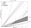 |
Fig. 7. Black hole masses of EXO 1846−031 obtained from X-ray observations. The black straight lines represent the black hole masses estimated using the RISCO derived from diskbb model fittings with NICER spectra, assuming the inclination range of 40° −74° and a non-spinning black hole. The dark grey region shows the mass range additionally satisfying the empirical condition of index transition luminosity estimated from the Swift/XRT spectrum. Each solid black curve in the bottom region indicates the constraint on black hole mass for different Eddington ratios (0.76%, 1.44%, and 2.75%) of the transition luminosity Ltran. The 90% confidence ranges are shown with accompanying dashed black curves. The solid curve marked with Lpeak/LEdd = 8% indicates the upper limit of mass estimated assuming the peak luminosity occurs at 8%LEdd and a high inclination of 74°. The colored straight lines represent the masses estimated using the RISCO and spin obtained from the diskbb+reflection models for X2, X3 and X4 observations. Their corresponding 90% confidence ranges are shown with accompanying dashed lines in the same colors. The red star mark the black hole masses suggested by the kerrbb+relxillNS model (a = 0.998) for X3. For reference, the masses suggested by the kerrbb+relxillNS+gauss model (a = 0.998) for X3 and X4 are shown with colored diamonds. |
If the central object was assumed as a rotating black hole, the black hole mass can be obtained using the relativistic accretion disk model, kerrbb. We applied the kerrbb model to a typical disk-dominated NICER spectrum (ID: 2200760143) in the high-soft state, assuming the inclination of 40° and 74° respectively. When fitting spectrum, we used the same strategy described in Section 3.2, but letting the spin vary from –1 to 1. We found that the lower inclination prefers a minimum spin while the higher inclination suggests a maximum spin. The fitting results for the black hole masses are shown in Figure 7. Considering the considerable hydrogen column density NH ∼ 6.1 × 1022 cm−2 , the extremely smaller source distance suggested by the high inclination set is less likely to be supported. Moreover, the masses suggested by high inclination exceed the upper limit of mass suggested by the peak luminosity when using NICER data.
With respect to mass constraints using broad spectra with reflection models, for the diskbb+reflection models, the black hole mass can be estimated using the relationship between RISCO and the spin parameter (Zhang et al. 1997; see also Bardeen et al. 1972). This is expressed as:
 (3)
(3)
where  , A1 = 1 + (1 − a2)(1/3)[(1 + a)1/3 + (1 − a)1/3] and A2 = (3a2 + A12)1/2. The RISCO values can be derived from the disk normalization and inclination in diskbb+reflection model using Equation (1). The black hole mass constraints estimated from the best-fit models for X2, X3 and X4 observations are shown in Figure 7. In addition, we also marked the black hole masses obtained from the fitting results of kerrbb+relxillNS model (observation X3, a = 0.998) and kerrbb+relxillNS+gauss model (observations X3 and X4, a = 0.998) for reference. Following the discussions in Section 4.1 and Section 4.2, the masses obtained from X3, fitted with kerrbb+relxillNS model (a = 0.998), should be prioritized, taking the physical meaning and the consistency of intrinsic parameters (i.e., inclination and spin) into consideration. The
  suggested by X3 fittings is also consistent with the mass obtained in Nath et al. (2024)’s work using TCAF model. There is no solution for the black hole mass that can satisfy the diskbb/kerrbb+reflection models and the Eddington mass ratio in the index transition simultaneously. If the mass obtained from the kerrbb+reflection model was the true case, the difference could be caused by a higher transition luminosity occurring at a date earlier than that suggested by MAXI and Swift observations. Alternatively, it could be due to the fact that the index transition of EXO 1846−031 occurred at a smaller Eddington ratio, compared to the empirical value.
5. Conclusions
We studied the X-ray properties of the 2019 outburst of the black hole candidate, EXO 1846−03, using NICER/XTI, NuSTAR, and HXMT data. According to the NICER spectral fittings, the state evolution from the low-hard to the high-soft and then back to the low-hard were observed during the outburst. In the very beginning of the outburst, a Comptonized model is preferred in describing the nonthermal component, rather than a simple power-law component, and a truncated disk is suggested. The large rin values indicated by the best-fit model (diskbb+relxill) of the simultaneous NICER and NuSTAR spectra in X1 observation also confirm the recession of the accretion disk in the low-hard state.
Currently the precise systematic parameters (i.e., inclination and mass) of EXO1846−031 are either lacking or strictly model-dependent. Before attempting to obtain the black hole mass constraint, we examined the divergent values suggested in previous works for the inclination by fitting the broad spectra with reflection models. A lower inclination of i < 55° was suggested according to the fitting results. Moreover, the extremely small source distance suggested by our NICER spectral fittings using a relativistic accretion disk in the high-soft state diminishes the possibility of a high inclination case, considering a conflict in terms of the considerable hydrogen column density for this source. The very high spin a > 0.98 obtained in Draghis et al. (2020) is not confirmed in our fittings with reflection model, while the retrograde case is unlikely to be supported.
We also discuss the allowed mass ranges estimated from different models. To complement the discussions on the mass constraint of the central object, we partially analyzed the MAXI and Swift/XRT data in the period when EXO 1846 − 031 transferring from the high-soft state toward the low-hard state when the NICER, NuSTAR, and HXMT observations were not available. A less model-dependent constraint on black hole mass is estimated to M < 8.2 M⊙ for a suggested source distance of 2.4 − 7.5 kpc. Assuming a maximum spin (a = 0.998) and adopting the complex model consisting of a relativistic disk and a reflection model (kerrbb+relxillNS) to the HXMT spectra, whose disk is obviously dominant, reveals a black hole of  at 7kpc. A more condensed black hole mass constraint required the improved estimates of inclination, spin, and the transition luminosity in further investigations and future observations of the source that are not limited to the X-ray band.
Reflection models are powerful tool that are frequently used to estimate the spin and inclination, although the complexity of the model and the unclarified reflection mechanism often require assumptions and simplifications when using those reflection models. This potentially leads to the divergent parameter estimates, for example the inclination of EXO 1846−031. A high spin is actually more frequently suggested by the reflection models (Draghis et al. 2024), while only a few systems with a negative (or consistent with a negative) spin have been revealed (see, e.g., Rout et al. 2020). However, theoretical works are more likely to predict a natal or randomly distributed spin (King & Kolb 1999; McClintock et al. 2006). We were attempting to reduce the model dependence and to obtain a more valid fitting parameters by considering the consistency among observations and vacating the unphysical cases (or cases displaying a conflict with empirical evidence), which was challenging. The development of reflection theories and numerical models in future would be helpful in working to obtain more credible information on X-ray sources with observation data and vice versa.
Acknowledgments
Authors are grateful for the support provided by the NICER, NuSTAR, HXMT, MAXI and Swift/XRT. Authors also appreciate the useful suggestions provided by the unknown referee.
References
- Bardeen, J. M., Press, W. H., & Teukolsky, S. A. 1972, ApJ, 178, 347 [Google Scholar]
- Bult, P. M., Gendreau, K. C., Arzoumanian, Z., et al. 2019, ATel., 12976, 1 [Google Scholar]
- Burnham, K. P., & Anderson, D. R. 2002, Model selection and multimodel inference: A practical information-theoretic approach (New York: Springer-Verlag) [Google Scholar]
- Connors, R. M. T., García, J. A., Dauser, T., et al. 2020, ApJ, 892, 47 [NASA ADS] [CrossRef] [Google Scholar]
- Cunningham, C. 1976, ApJ, 208, 534 [NASA ADS] [CrossRef] [Google Scholar]
- Draghis, P. A., Miller, J. M., Cackett, E. M., et al. 2020, ApJ, 900, 78 [NASA ADS] [CrossRef] [Google Scholar]
- Draghis, P. A., Miller, J. M., Costantini, E., et al. 2023, ArXiv e-prints [arXiv:2311.16225] [Google Scholar]
- Draghis, P. A., Miller, J. M., Costantini, E., et al. 2024, ApJ, 969, 40 [NASA ADS] [CrossRef] [Google Scholar]
- Emmanoulopoulos, D., Papadakis, I. E., Epitropakis, A., et al. 2016, MNRAS, 461, 1642 [NASA ADS] [CrossRef] [Google Scholar]
- Fragile, P. C., Ballantyne, D. R., Maccarone, T. J., & Witry, J. W. L. 2018, ApJ, 867, L28 [CrossRef] [Google Scholar]
- García, J., Dauser, T., Lohfink, A., et al. 2014, ApJ, 782, 76 [Google Scholar]
- García, J. A., Steiner, J. F., McClintock, J. E., et al. 2015, ApJ, 813, 84 [Google Scholar]
- García, J. A., Dauser, T., Ludlam, R., et al. 2022, ApJ, 926, 13 [CrossRef] [Google Scholar]
- George, I. M., & Fabian, A. C. 1991, MNRAS, 249, 352 [Google Scholar]
- King, A. R., & Kolb, U. 1999, MNRAS, 305, 654 [NASA ADS] [CrossRef] [Google Scholar]
- Kubota, A., & Makishima, K. 2004, ApJ, 601, 428 [Google Scholar]
- Kubota, A., Tanaka, Y., Makishima, K., et al. 1998, PASJ, 50, 667 [NASA ADS] [CrossRef] [Google Scholar]
- Lewin, W. H. G., van Paradijs, J., & van den Heuvel, E. P. J. 1995, Cambridge Astrophys. Series, 26 [Google Scholar]
- Li, L.-X., Zimmerman, E. R., Narayan, R., & McClintock, J. E. 2005, ApJS, 157, 335 [NASA ADS] [CrossRef] [Google Scholar]
- Lightman, A. P., & White, T. R. 1988, ApJ, 335, 57 [NASA ADS] [CrossRef] [Google Scholar]
- Liu, H.-X., Huang, Y., Xiao, G.-C., et al. 2021, Res. Astron. Astrophys., 21, 070 [Google Scholar]
- Makishima, K., Maejima, Y., Mitsuda, K., et al. 1986, ApJ, 308, 635 [NASA ADS] [CrossRef] [Google Scholar]
- McClintock, J. E., Shafee, R., Narayan, R., et al. 2006, ApJ, 652, 518 [NASA ADS] [CrossRef] [Google Scholar]
- Merloni, A., Fabian, A. C., & Ross, R. R. 2000, MNRAS, 313, 193 [NASA ADS] [CrossRef] [Google Scholar]
- Miller, J. M. 2007, ARA&A, 45, 441 [NASA ADS] [CrossRef] [Google Scholar]
- Miller, J. M., Zoghbi, A., Gandhi, P., & Paice, J. 2019, ATel., 13012, 1 [Google Scholar]
- Mitsuda, K., Inoue, H., Koyama, K., et al. 1984, PASJ, 36, 741 [NASA ADS] [Google Scholar]
- Nath, S. K., Debnath, D., Chatterjee, K., et al. 2024, ApJ, 960, 5 [Google Scholar]
- Negoro, H., Nakajima, M., Sugita, S., et al. 2019, ATel., 12968, 1 [Google Scholar]
- Parmar, A. N., & White, N. E. 1985, IAU Circ., 4051, 1 [NASA ADS] [Google Scholar]
- Parmar, A. N., Angelini, L., Roche, P., & White, N. E. 1993, A&A, 279, 179 [NASA ADS] [Google Scholar]
- Petrov, B. N., & Csáki, F. 1973, in 2nd International Symposium on Information Theory, Tsahkadsor, Armenia, USSR, September 2–8 (Akadémiai Kiadó), 1971 [Google Scholar]
- Reis, R. C., Fabian, A. C., & Miller, J. M. 2010, MNRAS, 402, 836 [NASA ADS] [CrossRef] [Google Scholar]
- Ren, X. Q., Wang, Y., Zhang, S. N., et al. 2022, ApJ, 932, 66 [NASA ADS] [CrossRef] [Google Scholar]
- Rout, S. K., Vadawale, S., & Méndez, M. 2020, ApJ, 888, L30 [Google Scholar]
- Shafee, R., McClintock, J. E., Narayan, R., et al. 2006, ApJ, 636, L113 [NASA ADS] [CrossRef] [Google Scholar]
- Shakura, N. I., & Sunyaev, R. A. 1973, A&A, 24, 337 [NASA ADS] [Google Scholar]
- Shimura, T., & Takahara, F. 1995, ApJ, 445, 780 [Google Scholar]
- Steiner, J. F., Narayan, R., McClintock, J. E., & Ebisawa, K. 2009, PASP, 121, 1279 [Google Scholar]
- Steiner, J. F., McClintock, J. E., & Narayan, R. 2013, ApJ, 762, 104 [Google Scholar]
- Wang, S., Kawai, N., Shidatsu, M., et al. 2018, PASJ, 70, 67 [Google Scholar]
- Wang, Y., Ji, L., García, J. A., et al. 2021, ApJ, 906, 11 [CrossRef] [Google Scholar]
- Wang, S., Kawai, N., Shidatsu, M., & Matsuoka, Y. 2023, PASJ, 75, 1072 [Google Scholar]
- Williams, D. R. A., Motta, S. E., Fender, R., et al. 2022, MNRAS, 517, 2801 [Google Scholar]
- Wilms, J., Allen, A., & McCray, R. 2000, ApJ, 542, 914 [Google Scholar]
- Zhang, S. N., Cui, W., & Chen, W. 1997, ApJ, 482, L155 [NASA ADS] [CrossRef] [Google Scholar]
- Zhang, S.-N., Li, T., Lu, F., et al. 2020, Sci. China Phys. Mech. Astron., 63, 249502 [NASA ADS] [CrossRef] [Google Scholar]
- Życki, P. T., Done, C., & Smith, D. A. 1999, MNRAS, 309, 561 [Google Scholar]
Appendix A: Fitting comparisons with reflection models for X2, X3, and X4
 |
Fig. A.1. Fitting results with reflection models (a = 0.998) using joint NICER+NuSTAR spectra and HXMT spectra. The bins in each figure are plotted that have at least 50 sigma, or are grouped in sets of five bins, to make the goodness of fit easier to compare. |
Appendix B: Examples of reflection spectra for X2, X3, and X4
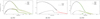 |
Fig. B.1. Spectral shapes of X2, X3, and X4. Here we used the diskbb+relxill model as example. The bins in each figure are plotted that have at least 50 sigma or are grouped in sets of five bins to make the spectral shape easier to see. |
Appendix C: The kerrbb+relxillNS spectra for X2 and X4
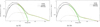 |
Fig. C.1. Spectra fitted with kerrbb+relxillNS model for X2, and X4. The bins in each figure are plotted that have at least 50 sigma or are grouped in sets of five bins to make the spectral shape easier to see. |
Appendix D: HXMT spectra with the kerrbb+reflection+gauss models (a = 0.998)
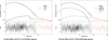 |
Fig. D.1. X3 spectra with the kerrbb+reflection+gauss models. The bins in each figure are plotted that have at least 50 sigma, or are grouped in sets of five bins, to make the goodness of fit easier to compare. |
D.1. Bolometric flux of Index transition
We analyzed the MAXI and Swift data to determine the flux of the transition toward the low-hard state for EXO 1846−031 during its 2019 outburst. For MAXI data, we constructed MAXI spectra using the MAXI on-demand tool5 with a 1 arcmin circle for the source region and a 3 arcmin circle for the background region. During the bright phase before MJD 58775, each MAXI spectrum was extracted with a 5-day time interval. From MJD 58775 to MJD 58860, each MAXI spectrum was extracted with a 10-day time interval. After MJD 58860, the MAXI spectrum was extracted with a 20-day time interval to obtain a reasonable statistic. We also checked the available Swift/XRT data in the later half of the outburst and constructed energy spectrum for each Swift observation ID using the online tool6 with the setting of grade-zero event. We adopted the energy range of 2−20 keV to MAXI spectra and the energy range 1 − 10 keV to Swift spectra. Prior to spectral fittings, the adjacent energy bins in each Swift/XRT spectrum were grouped to satisfy a 30 photon counts threshold. The MAXI and Swift spectra whose statistics are poorer than 50 data points per spectrum were excluded since it is hard to constrain the spectral parameters. All MAXI and Swift spectra were fitted with a tBabs × (diskbb + power-law) model with NH fixed to 6.1 × 1022 cm−2. Figure D.2 shows the fitting results of MAXI and Swift spectra. Although there are considerable uncertainties of MAXI spectral index, the index shows decreasing trend after MJD 58900, which can be assumed as the index transition to the low-hard state. To validate the photon index drop tendency, in the end of the outburst we additionally show the result of one MAXI spectrum (MJD 58915 − MJD58935) fitted with the power-law model, which suggests a smaller photon index ∼1.8. This low photon index more or less supports the assumption of MJD 58900 as the index transition date toward the low-hard state, although the additional MAXI spectrum has a less quality statistic (∼20 data points). Since the Swift data are available during the period of MJD 58900 − MJD 58920, and are able to provide better statistics with comparatively smaller time interval, we employed the bolometric power-law flux estimated from the first Swift spectrum right after MJD 58900 as the transition flux.
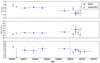 |
Fig. D.2. Spectral parameter variations of inner disk temperature (Tin), disk normalization and photon index (Γ), using the diskbb+power-law model for MAXI and Swift/XRT observations. MAXI data are represented by blue triangles and Swift/XRT data are represented by open circles. The last open triangle in the bottom panel shows the photon index of the MAXI spectrum (MJD 58915− MJD58935) fitted with a simple power-law model. The dashed line indicates the index transition deduced from MAXI and Swift/XRT spectral fittings. |
Appendix E: Tables of the fitting results with reflection models
Fitting results with diskbb+reflection model
Fitting results with kerrbb+reflection model
All Tables
NICER, NuSTAR and HXMT observations of EXO 1846−031 used in reflection model fittings.
All Figures
|
Fig. 1. Light curves and hardness ratios of EXO 1846−031 during its 2019 outburst as functions of MJD. Top panel shows the light curves in the soft bands: 0.3 − 4 keV for NICER/XTI and Swift/XRT; 2 − 4 keV for MAXI/GSC. Middle panel shows the light curves in hard bands: 4 − 6 keV for NICER/XTI, 4 − 10 keV for Swift/XRT and MAXI/GSC. Bottom panel shows the corresponding hardness ratio for NICER/XTI (4 − 6 keV/0.3 − 4 keV), Swift/XRT (4 − 10 keV/0.3 − 4 keV), and MAXI/GSC (4 − 10 keV/2 − 4 keV), respectively. The NICER (black circles) and Swift data (open circles) are depicted on the left y-axis, and the MAXI data (blue triangles) are depicted on the right y-axis. The green and red bars represent the times of the NuSTAR and HXMT observations. |
| In the text | |
|
Fig. 2. Panel (a) shows the NICER spectrum (ID 2200760101) fitted with TBabs*(simpl*diskbb+gauss)*edge. The dotted line represent the Gaussian component. Panel (b) shows the residuals in terms of sigma for the model, TBabs*(simpl*diskbb). Panel (c) shows the residuals for the model, TBabs*(simpl*diskbb)*edge. Panel (d) gives the best-fit model, TBabs*(simpl*diskbb+gauss)*edge. |
| In the text | |
|
Fig. 3. Evolution of fitting parameters of NICER spectra during the 2019 outburst of EXO 1846 − 031. From top to bottom, each panel shows the innermost disk temperature, the normalization of disk, the photon index, and the reduced χ2, respectively. The arrows in the top panel point the simultaneous NuSTAR observations and the dashed arrow points the date of HXMT observation used in this study. |
| In the text | |
|
Fig. 4. Evolution paths of the innermost disk radii. The blue crosses represent the rin estimated from the fitting results with diskbb+NthComp model and the black crosses represent the rin corrected using Equation (1). |
| In the text | |
|
Fig. 5. Simultaneous NuSTAR/FPMA and NICER/XTI spectra at MJD 58698.1 fitted with a complex model of constant*TBabs*(diskbb+power-law). The black data points represent the NICER/XTI (1.3–10 keV) spectrum with observation ID 2200760104. The green data points represent the NuSTAR/FPMA spectrum (4–79 keV) with the observation ID 90501334002. The red data points represent the NuSTAR/FPMA spectrum with the same NuSTAR observation ID as that of green points but having the exactly same observation period as that of NICER spectrum. |
| In the text | |
|
Fig. 6. Joint NICER+NuSTAR spectrum fitted with the diskbb+relxill+cutoff power-law model for X1 observation, where the NICER data is marked in black, NuSTAR/FPMA is marked in red and NuSTAR/FPMB is marked in green. The disk component is represented by dotted line, the nonthermal component is represented by dashed line and the reflection model is represented by solid line. The goodness of fit with diskbb+cutoffpl model is shown in the bottom panel for compassion. The bins in the figure are plotted that have at least 50 sigma, or are grouped in sets of five bins, to make the goodness of fit easier to compare. |
| In the text | |
|
Fig. 7. Black hole masses of EXO 1846−031 obtained from X-ray observations. The black straight lines represent the black hole masses estimated using the RISCO derived from diskbb model fittings with NICER spectra, assuming the inclination range of 40° −74° and a non-spinning black hole. The dark grey region shows the mass range additionally satisfying the empirical condition of index transition luminosity estimated from the Swift/XRT spectrum. Each solid black curve in the bottom region indicates the constraint on black hole mass for different Eddington ratios (0.76%, 1.44%, and 2.75%) of the transition luminosity Ltran. The 90% confidence ranges are shown with accompanying dashed black curves. The solid curve marked with Lpeak/LEdd = 8% indicates the upper limit of mass estimated assuming the peak luminosity occurs at 8%LEdd and a high inclination of 74°. The colored straight lines represent the masses estimated using the RISCO and spin obtained from the diskbb+reflection models for X2, X3 and X4 observations. Their corresponding 90% confidence ranges are shown with accompanying dashed lines in the same colors. The red star mark the black hole masses suggested by the kerrbb+relxillNS model (a = 0.998) for X3. For reference, the masses suggested by the kerrbb+relxillNS+gauss model (a = 0.998) for X3 and X4 are shown with colored diamonds. |
| In the text | |
|
Fig. A.1. Fitting results with reflection models (a = 0.998) using joint NICER+NuSTAR spectra and HXMT spectra. The bins in each figure are plotted that have at least 50 sigma, or are grouped in sets of five bins, to make the goodness of fit easier to compare. |
| In the text | |
|
Fig. B.1. Spectral shapes of X2, X3, and X4. Here we used the diskbb+relxill model as example. The bins in each figure are plotted that have at least 50 sigma or are grouped in sets of five bins to make the spectral shape easier to see. |
| In the text | |
|
Fig. C.1. Spectra fitted with kerrbb+relxillNS model for X2, and X4. The bins in each figure are plotted that have at least 50 sigma or are grouped in sets of five bins to make the spectral shape easier to see. |
| In the text | |
|
Fig. D.1. X3 spectra with the kerrbb+reflection+gauss models. The bins in each figure are plotted that have at least 50 sigma, or are grouped in sets of five bins, to make the goodness of fit easier to compare. |
| In the text | |
|
Fig. D.2. Spectral parameter variations of inner disk temperature (Tin), disk normalization and photon index (Γ), using the diskbb+power-law model for MAXI and Swift/XRT observations. MAXI data are represented by blue triangles and Swift/XRT data are represented by open circles. The last open triangle in the bottom panel shows the photon index of the MAXI spectrum (MJD 58915− MJD58935) fitted with a simple power-law model. The dashed line indicates the index transition deduced from MAXI and Swift/XRT spectral fittings. |
| In the text | |
Current usage metrics show cumulative count of Article Views (full-text article views including HTML views, PDF and ePub downloads, according to the available data) and Abstracts Views on Vision4Press platform.
Data correspond to usage on the plateform after 2015. The current usage metrics is available 48-96 hours after online publication and is updated daily on week days.
Initial download of the metrics may take a while.