| Issue |
A&A
Volume 704, December 2025
|
|
|---|---|---|
| Article Number | A182 | |
| Number of page(s) | 20 | |
| Section | Planets, planetary systems, and small bodies | |
| DOI | https://doi.org/10.1051/0004-6361/202453323 | |
| Published online | 09 December 2025 | |
The mid-infrared spectrum of β Pictoris b
First VLTI/MATISSE interferometric observations of an exoplanet★
1
Univ. Côte d’Azur, Observatoire de la Côte d’Azur, CNRS, Laboratoire Lagrange,
Nice,
France
2
Univ. Grenoble Alpes, CNRS, IPAG,
38000
Grenoble,
France
3
LESIA, Observatoire de Paris, PSL, CNRS, Sorbonne Univ., Univ. de Paris,
5 place Janssen,
92195
Meudon,
France
4
European Southern Observatory,
Karl-Schwarzschild-Straße 2,
85748
Garching,
Germany
5
Max-Planck-Institut für Astronomie,
Königstuhl 17,
69117
Heidelberg,
Germany
6
Institute of Astronomy, Univ. of Cambridge,
Madingley Road,
Cambridge
CB3 0HA,
UK
7
Université Paris-Saclay, Univ. Paris Cité, CEA, CNRS, AIM,
91191
Gif-sur-Yvette,
France
8
Department of Physics & Astronomy, Johns Hopkins Univ.,
3400 N. Charles Street,
Baltimore,
MD
21218,
USA
9
Space Telescope Science Institute,
3700 San Martin Drive,
Baltimore,
MD
21218,
USA
10
Leiden Observatory, Leiden Univ.,
PO Box 9513,
2300
RA
Leiden,
The Netherlands
11
European Southern Observatory,
Alonso de Córdova 3107, Casilla 19, Vitacura,
Santiago,
Chile
12
Univ. of Exeter, Physics Building,
Stocker Road,
Exeter
EX4 4QL,
UK
13
Anton Pannekoek Institute for Astronomy, University of Amsterdam,
Science Park 904,
1098
XH
Amsterdam,
The Netherlands
14
European Space Agency (ESA), ESA Office, Space Telescope Science Institute,
3700 San Martin Drive,
Baltimore,
MD
21218,
USA
15
Konkoly Observatory, Research Centre for Astronomy and Earth Sciences, HUN-REN,
Konkoly-Thege Miklós út 15–17,
1121
Budapest,
Hungary
16
CSFK, MTA Centre of Excellence, Budapest,
Konkoly Thege Miklós út 15–17,
1121
Budapest,
Hungary
17
Aix Marseille Univ., CNRS, CNES, LAM,
Marseille,
France
18
Center for Interdisciplinary Exploration and Research in Astrophysics (CIERA) and Department of Physics and Astronomy, Northwestern Univ.,
Evanston,
IL
60208,
USA
19
Max-Planck-Institut für Radioastronomie,
Auf dem Hügel 69,
53121
Bonn,
Germany
★★ Corresponding author: This email address is being protected from spambots. You need JavaScript enabled to view it.
Received:
6
December
2024
Accepted:
25
August
2025
Abstract
Few spectra of directly imaged exoplanets have been obtained in the mid-infrared (>3 μm). This region is particularly rich in molecular spectral signatures, whose measurements can help recover atmospheric parameters and provide a better understanding of giant planet formation and atmospheric dynamics. In recent years, exoplanet interferometry with the VLTI/GRAVITY instrument has provided medium-resolution spectra of a dozen sub-stellar companions in the near-infrared. The 100 meter interferometric baselines enable the stellar and planetary signals to be efficiently disentangled at close angular separations (<0.3″). We aim to extend this technique to the mid-infrared using MATISSE, the VLTI’s mid-infrared spectro-interferometer. We take advantage of the fringe tracking and off-axis pointing capabilities recently brought by the GRA4MAT upgrade. Using this new mode, we observed the giant planet β Pictoris b in L and M bands (2.75–5 μm) at a spectral resolution of 500. We developed a method to correct chromatic dispersion and non-common path effects in the fringe phase and modelled the planet astrometry and stellar contamination. We obtained a high-signal-to-noise spectrum of β Pictoris b, showing the planet continuum in the L (for the first time) and M bands, which contains broad absorption features of H2O and CO. In conjunction with a new GRAVITY spectrum, we modelled it with the ForMoSA nested sampling tool and the Exo-REM grid of atmospheric models, and found a solar carbon-to-oxygen ratio in the planet atmosphere. This study opens the way to the characterization of fainter and closer-in planets with MATISSE, which could complement the JWST at angular separations too close for it to obtain exoplanet spectra. Starting in 2025, the new adaptive optics system brought by the GRAVITY+ upgrade will further extend the detection limits of MATISSE.
Key words: techniques: interferometric / planets and satellites: atmospheres / planets and satellites: formation / planets and satellites: gaseous planets / infrared: planetary systems
Based on public data released from the MATISSE commissioning observations at the VLT Interferometer under ESO Programme 60.A-9257(H), and NACO observations under ESO Programme 088.C-0196.
© The Authors 2025
 Open Access article, published by EDP Sciences, under the terms of the Creative Commons Attribution License (https://creativecommons.org/licenses/by/4.0), which permits unrestricted use, distribution, and reproduction in any medium, provided the original work is properly cited.
This article is published in open access under the Subscribe to Open model. This email address is being protected from spambots. You need JavaScript enabled to view it. to support open access publication.
1 Introduction
The emission of massive Jovian companions detected by highcontrast imaging can now be characterized in detail from ultraviolet (HST, Zhou et al. 2014; VLT/XSHOOTER, Petrus et al. 2020) to mid-infrared wavelengths (JWST/NIRSpec, 0.70–5.27 μm, Böker et al. 2022; JWST/MIRI, 4.9–27.9 μm, Wells et al. 2015; Argyriou et al. 2023). The mid-infrared is a rich spectral window for exoplanetary atmospheres, as has been hinted at by recent advances in atmospheric modelling: thanks to absorption features of molecules such as CO, CH4, CO2, or H2O, it may encode information about cloud thickness (Charnay et al. 2018), vertical mixing and induced disequilibrium chemistry (Phillips et al. 2020), or the heterogeneity of the cloud cover (Currie et al. 2014). It can help to model the dust environment of young accreting planets, in particular the temperature, radius, and mass of their circumplanetary discs (Wang et al. 2021b; Cugno et al. 2024). Finally, it can possibly hint at auroral signatures in cold planets and brown dwarfs through the detection of CH4 emission (Faherty et al. 2024). The mid-infrared also has technical advantages: the planet-to-star contrast is lower (e.g. ~4× lower in L′ than in K for β Pic b, Lagrange et al. 2009; Bonnefoy et al. 2011); the atmospheric turbulence has longer coherence lengths and timescales; and the Strehl ratio is higher. The sky emission, however, is higher in the mid-infrared.
One of the first direct emission spectra of an unambiguous1 exoplanet was obtained in the L band (HR 8799 c with VLT/NACO, Janson et al. 2010). Since then, although mid-infrared photometry has been obtained for many companions, only a few other mid-infrared spectra of directly imaged planets from ground-based telescopes have been published. The list hereafter is exhaustive to the best of our knowledge. High-resolution spectra (R = λ/Δλ > 15 000) were obtained in the L (HR 8799 c, Wang et al. 2018; β Pic b, Janson et al. 2025) and M bands (β Pic b, Parker et al. 2024). High-resolution spectroscopy gives access to many individual spectral lines that can be cross-correlated with molecular template spectra, but not to the spectral energy distribution (SED) of the planet. At low resolution (R = 35), Doelman et al. (2022) presented L-band spectra of HR 8799 c, d, and e with the LBTI/ALES integral field spectrograph, showing their SEDs including broad absorption features. Low- or medium-resolution L-band spectra were also obtained for three isolated or widely separated planetary-mass objects (Miles et al. 2018; Stone et al. 2020). This low number of mid-infrared spectra obtained from the ground may be due to the scarcity of mid-infrared spectrographs assisted by adaptive optics (AO) on 8 m-class telescopes, as high-contrast instruments with extreme AO systems have been developed in the H and K bands so far (VLT/SPHERE, Gemini/GPI, and Subaru/SCExAO, Beuzit et al. 2019; Macintosh et al. 2014; Jovanovic et al. 2015).
More recently, from space, the JWST provided a broad 1–20 μm spectrum of the widely separated (8″) companion VHS 1256-1257 b (Miles et al. 2023; Petrus et al. 2024) and a 5–7 μm spectrum of β Pic b (Worthen et al. 2024). Simulations using molecular mapping or forward modelling techniques applied to the IFU on board the instruments have shown detection limits down to 0.5″ with MIRI (Patapis et al. 2022; Mâlin et al. 2023) and 0.3″ (at constrasts down to 3 × 10⁻⁵) with NIR-Spec (Ruffio et al. 2024). However, characterization below these separations (<3 spaxels and 3λ/D from the host star) remains untested so far, as does the ability to extract the SED of the companion, which is not recovered in molecular mapping.
A push towards spectroscopy at closer angular separations has recently come from ground-based long-baseline interferometry. A dozen planets have been observed with the near-infrared GRAVITY instrument (GRAVITY Collaboration 2017) on the Very Large Telescope Interferometer (see e.g. GRAVITY Collaboration 2019; GRAVITY Collaboration 2020). This has led to precise astrometric measurements enabling well-constrained orbital fits, as well as near-infrared K-band spectra at R = 500, including for companions at separations <0.2″ unreachable by integral field spectrographs (β Pic c, Nowak et al. 2020; HD 206893 c, Hinkley et al. 2023). The 100 m baselines of the VLTI help to efficiently disentangle stellar and planetary photons, providing spectra at close separations and medium spectral resolutions that retain the planet continuum, while resolving some spectral lines.
To extend this capability to the mid-infrared, a new observing strategy, GRA4MAT (Woillez et al. 2024), has been developed to increase the sensitivity of MATISSE, the VLTI’s mid-infrared spectro-interferometer (Lopez et al. 2022). In GRA4MAT, while MATISSE performs science observations, the GRAVITY fringe tracker (Lacour et al. 2019; Nowak et al. 2024) measures the rapidly varying optical path difference (OPD) between telescope light paths introduced by atmospheric turbulence, and corrects the OPD using the VLTI delay lines (instead of GRAVITY’s internal delay lines in a classical GRAVITY observation, GRAVITY Collaboration 2017). As a result, fringes are stabilized for MATISSE in the L, M, and N bands. The narrow off-axis mode adds the possibility of offsetting MATISSE’s optical axis from the fringe tracking source. These implementations lead to two huge improvements in sensitivity: 1) MATISSE can now expose 90× longer than the short exposure times previously required to freeze the turbulence (10 s vs 111 ms), making MATISSE background-limited instead of detector-limited; and 2) by centring MATISSE on the planet, most of the stellar photons fall outside MATISSE’s spatial filter (a 135 mas pinhole, or 1.5λ/D at 3.5 μm), reducing the stellar contamination. A simulation of this effect for the case of β Pic b, with a planet-to-star contrast of 8 × 10⁻⁴ at a separation of 534 mas, is shown in Fig. 1, assuming no turbulence and perfect telescopes. When centred on the planet, the pinhole reduces the speckle flux to the same level as the planetary flux at the planet position.
To demonstrate this new observing window to exoplanets, we observed the iconic β Pictoris b, a giant planet discovered through L′-band imaging at 8 au from its star (Lagrange et al. 2009) inside an edge-on debris disc (Smith & Terrile 1984; Hobbs et al. 1985). β Pictoris is one of the most studied extrasolar planetary systems, whether through direct imaging (Lagrange et al. 2019a; Kammerer et al. 2024), radial velocities hinting at the inner companion β Pic c at 2.7 au (Lagrange et al. 2019b), high-resolution spectroscopy uncovering the fast spin of β Pic b (~20 km/s, Snellen et al. 2014; Landman et al. 2024; Parker et al. 2024), host star astrometry (Snellen & Brown 2018), low- and medium-resolution spectroscopy in the J, H, and M bands (Chilcote et al. 2017; Worthen et al. 2024), molecular mapping with integral field spectroscopy (Hoeijmakers et al. 2018; Kiefer et al. 2024), or K-band spectro-interferometry directly confirming β Pic c (GRAVITY Collaboration 2020; Nowak et al. 2020). The dynamical mass of β Pic b has been constrained from orbital fits of these numerous observations, first using the host star astrometry (Snellen & Brown 2018; Dupuy et al. 2019), then adding radial velocity measurements and planetary astrometry from imaging and interferometry (GRAVITY Collaboration 2020; Vandal et al. 2020; Lagrange et al. 2020; Lacour et al. 2021; Brandt et al. 2021). Dynamical mass estimates from these studies range from 9 to 13 MJup. With a flux of 8 mJy (Lagrange et al. 2009), β Pic b is the brightest imaged exoplanet in the L band thanks to its proximity (19.44 ± 0.05 pc, Nielsen et al. 2020) and high temperature of ~1500–1700 K (corresponding to an early L spectral type, Bonnefoy et al. 2013; GRAVITY Collaboration 2020). Although it was discovered in the L′ band, it is still missing an SED in this region. This makes it a prime target for a first demonstration of MATISSE capabilities.
We present in Section 2 the outline of the MATISSE observations of β Pic b. We explain our data reduction in Section 3, including additional steps to the standard MATISSE pipeline. The astrometry and spectrum of the planet is extracted from the reduced data in Section 4. We analyse the spectrum with forward modelling in Section 5, discuss our results in Section 6, and conclude in Section 7.
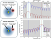 |
Fig. 1 Simulation of the gain in contrast achieved by offsetting the pinhole of MATISSE on β Pic b, separated here by 534 mas from its host star. The upper and lower plots depict the stellar and planetary contribution to the coherent flux (the fringe envelope) as seen through the circular MATISSE pinhole (white area, hence the Airy-like shape of the output flux) centred on the star and on the planet, respectively. They are simulated at a wavelength of 3.5 μm and normalized to the maximal intensity of the star-centred stellar PSF. When the pinhole is centred on the planet, the speckle flux is reduced to the same level as the planetary flux. In each simulation, the asymmetric shape of the PSF of the offset object (relative to the pinhole) is due to imperfect spatial filtering of the Airy rings falling in the pinhole. |
Observing log.
2 Observations
β Pic b was observed with MATISSE during the commissioning of the GRA4MAT narrow off-axis mode (Woillez et al. 2024), on the nights of November 8, 2022 and February 3, 20232. We obtained observations at R = 500 between 2.75 and 5 μm, covering the full L band (2.8–4.2 μm) and the blue side of the M band (4.5–5 μm). The planet position was predicted with whereistheplanet3 (Wang et al. 2021a), which uses orbital fits of archival planet astrometry (Lacour et al. 2021) with the orbitize! package (Blunt et al. 2020). We followed two different observing sequences in November 2022 and February 2023, summarized in Table 1. In November 2022, we alternated for 2 h between two or three cycles targeting the planet and one targeting the star. A cycle consists of four successive exposures using each of MATISSE’s beam commuting device (BCD) configurations. The total exposure time amounts to 44 min on the planet and 16 min on the star. As is explained in Sect. 3.1, the stellar pointings are used to calibrate the telluric contamination and anchor the stellar contribution to the stellar pointing in the planet observations. In February 2023, we added a so-called ‘anti-planet’ pointing at the opposite position of β Pic b with respect to the star, in order to confirm the astrophysical nature of the signal recorded on the planet. This shorter observation amounted to one cycle on the star (4 min), two on the planet (8 min), and one at the anti-planet position (4 min). We show in Appendix A a comparison of coherent flux ratios at the planet and anti-planet positions. As was expected, no planet-like signal is found at the anti-planet position. Given its short exposure time, higher seeing, higher water vapour, and for data homogeneity, we discard the 2023 dataset and focus on the 2022 dataset in the following sections.
3 Data reduction
In interferometry, the quantity of interest is the coherent flux (also known as complex correlated flux), a complex quantity describing the amplitude and phase of the interferometric fringe pattern. It encodes the Fourier transform of the source spatial brightness distribution, and is sampled by the interferometer at given spatial frequencies defined by the baseline length and orientation relative to the source. A general introduction of the technique can be found in, for example, Buscher (2015). The MATISSE pipeline reduces the fringe pattern images and extracts the coherent flux (Sect. 3.1). We developed custom reduction steps to correct for remaining instrumental and atmospheric effects (Sect. 3.2).
3.1 MATISSE and GRA4MAT standard pipeline
We used the standard MATISSE pipeline (version 2.0.24) in ‘correlated flux’ mode (option ––corrFlux=True) to reduce the observations. The fringes recorded by MATISSE are Fourier-transformed, providing the observer with a complex coherent flux for each frame. The frames are then carefully selected: MATISSE frames during which the GRA4MAT fringe tracker experienced a jump from one fringe to another (i.e. a phase jump of a 2π multiple) are discarded. This is necessary as the fringe tracking and science channels of GRA4MAT are in different bands: a 2π jump in K results in a very different jump in L that is generally not a multiple of 2π. Without knowledge of when jumps happen during a frame, this creates a highly variable fringe contrast that cannot be calibrated. It is therefore preferable to simply flag and remove these frames. In the November 2022 dataset, 60 out of the 360 frames had jumps (~17%). This proportion greatly improved after a later update of the fringe tracker (Nowak et al. 2024; Woillez et al. 2024): no frame was rejected in the February 2023 dataset.
After this selection, the MATISSE pipeline fits and removes in the coherent flux any residual phase created by an achromatic OPD, and coherently averages the frames over the duration of an exposure (1 min). After inspection of the final products, we note that the pipeline does not fully remove residual achromatic OPDs in L and M bands. It also does not correct for chromatic dispersion near the telluric absorption bands. For these reasons, we developed our own phase correction method described in the following subsection. This has the additional advantage of providing individual frame products instead of average exposure products. In this custom phase correction, we use the intermediate pipeline products nrjReal and nrjImag. They contain the real and imaginary parts of the coherent flux extracted from the raw interferogram, after correction of the bias, bad pixels and distortion, but before the achromatic OPD removal.
3.2 Custom steps
3.2.1 Phase correction
In interferometry, an OPD δ(λ) generates a shift of 2πδ(λ)/λ in the fringe phase. The GRA4MAT fringe tracker measures and compensates the K-band OPD originating in the line of sight of GRAVITY, i.e. in the common path of GRAVITY and MATISSE. Additional atmospheric and instrumental phase terms remain, however, as is shown in Fig. 2, an example of phase measurements in two on-star and on-planet frames before the pipeline OPD correction. As is explained in Sect. 4, the phase created by the targets should be zero when pointing at the star (characteristic of an unresolved point source), or be modulated by an oscillatory function of 1/λ when pointing at the planet (characteristic of a resolved binary source, here the stellar halo and the planet). As can be seen here, the actual measured phase contains two additional components: a linear term as function of 1/λ, and high-order terms near the telluric absorption bands defining the edges of the L and M bands. Linear terms should in principle be measured and removed by the fringe tracker. As it appears uncorrected by GRA4MAT, it must originate in a ‘non-common path’ achromatic OPD introduced between GRAVITY and MATISSE, which would be left unseen by the fringe tracker. It is so far only partially fitted and subtracted by the last recipe of the MATISSE pipeline. The high-order terms are created by chromatic variations in the air refractive index (i.e. chromatic dispersion) near the main telluric absorption bands (CO2 and H2O bands at ~2.7 μm, CO2 band at ~4.2 μm). We aim to correct both the non-common path (NCP) achromatic OPD and the common-path (CP) chromatic variations. A detailed demonstration of the method is presented in Appendix B. We present here a summary of the main points.
We first defined each of the OPDs introduced in the successive mediums along the common path: vacuum, atmosphere, and delay lines. We simulated these terms and their correction by the fringe tracker using an air refractive index model (Voronin & Zheltikov 2017) and pessimistic assumptions on the differences in ambient conditions between lines of sight. We found that one of these corrected OPDs, originating in the additional length travelled in space and its compensation by the delay lines in air, is more than ten times larger than the other terms in L and M bands, except at the bluer edge of the bands. This leads us to approximate the corrected common-path OPD as follows:
![Mathematical equation: $\[\delta_{\mathrm{CP}}^{\mathrm{corr}}(\lambda) \approx\left(\frac{n_{\mathrm{DL}}(\lambda)}{\left\langle n_{\mathrm{DL}}(\lambda)\right\rangle_K}-1\right) \Delta d,\]$](/articles/aa/full_html/2025/12/aa53323-24/aa53323-24-eq1.png) (1)
(1)
in which nDL(λ) is the air refractive index in the delay lines, ⟨nDL(λ)⟩K is its average in K band, and Δd is the additional length travelled in vacuum, compensated in the delay lines. Overall, our phase model after fringe tracking (Φcorr) is the sum of the target phase (Φobj) and the phases originating in the corrected common-path OPD and the non-common path OPD (δNCP):
![Mathematical equation: $\[\begin{aligned}\Phi^{\mathrm{corr}}(\lambda) & \approx \Phi_{\mathrm{obj}}(\lambda)+\frac{2 \pi}{\lambda}\left[\delta_{\mathrm{CP}}^{\mathrm{corr}}(\lambda)+\delta_{\mathrm{NCP}}\right] \\& \approx \Phi_{\mathrm{obj}}(\lambda)+\frac{2 \pi}{\lambda}\left[\left(\frac{n_{\mathrm{DL}}(\lambda)}{\left\langle n_{\mathrm{DL}}(\lambda)\right\rangle_K}-1\right) \Delta d+\delta_{\mathrm{NCP}}\right].\end{aligned}\]$](/articles/aa/full_html/2025/12/aa53323-24/aa53323-24-eq2.png) (2)
(2)
Before fitting this model to the data, we removed from both of them their mean L-band phase in order to get the differential phase, a standard step in interferometry when the absolute phase reference is lost during fringe tracking:
![Mathematical equation: $\[\Phi^{\mathrm{diff}}(\lambda)=\Phi^{\mathrm{corr}}(\lambda)-\left\langle\Phi^{\mathrm{corr}}(\lambda)\right\rangle_L.\]$](/articles/aa/full_html/2025/12/aa53323-24/aa53323-24-eq3.png) (3)
(3)
During our reduction, only the non-common path term δNCP was fitted. We found that an achromatic constant term per frame and baseline is sufficient to reproduce the data well. This likely stems from the differential dispersion between K and L bands, mostly due to water vapour variations; and from a possible slow instrumental drift between GRAVITY and MATISSE during the night, as the instruments are only aligned once before the observations. The common-path term is not fitted but modelled thanks to the path lengths and ambient conditions (temperature, pressure, and humidity) measured in the delay line tunnel and reported in the FITS header of the MATISSE frames. The ambient conditions are fed into air refractive index models, for which we tested three different ones. The model of Voronin & Zheltikov (2017) presents interesting features in comparison to previous widely used models: it takes into account the contribution of the wings of the main infrared absorption lines, which are not considered in Ciddor (1996), and enables the variation in the CO2 concentration (as well as other gases) contrary to the models of Mathar (2007) tabulated at a fixed value of 370 ppm, which is every year drifting away from the actual CO2 concentration (~417 ppm in 20225) rising from anthropogenic emissions. This is especially important in the L and M bands that are separated by a strong CO2 absorption feature.
We show in Fig. 2 the measured differential phase in two frames, one being centred on the star and the other on the planet. We overlay the fits of our model using the three different air refractive index formulae. The one of Voronin & Zheltikov (2017) is clearly favoured, providing a better fit across the L band including very close to the CO2 line at 4.2 μm. We note that in the planet data, the higher-frequency planet–star modulation does not affect the fit of δNCP, if bounds are provided on this term during the fit. We also note some discrepancies between model and data near the red L-band edge and in M band. They are likely caused by the OPD terms we neglected in Eq. (1), which originate in ambient condition differences between lines of sight in the atmosphere and the delay lines. These discrepancies appear almost constant between successive planet and star pointings. They are thus well removed by subtracting from each planet phase the average of the corrected stellar phases from the next observation block (OB). This step is inherently part of the calibration strategy presented in the next section. For this reason, a fit of the ambient condition differences in addition to δNCP does not seem to be required at the moment. This could nonetheless be the subject of further study if more precision is required. Our final estimate of the object differential phase is the difference between the measured differential phase and the fit, using the air refractive index of Voronin & Zheltikov (2017):
![Mathematical equation: $\[\Phi_{\mathrm{obj}}^{\mathrm{diff}}(\lambda) \approx \arg \left[\mathrm{e}^{\mathrm{i} \Phi^{\mathrm{diff}}(\lambda)} \mathrm{e}^{-\mathrm{i} \frac{2 \pi}{\lambda}\left(\delta_{\mathrm{CP}}^{\text {corr }}(\lambda)+\delta_{\mathrm{NCP}}\right)}\right].\]$](/articles/aa/full_html/2025/12/aa53323-24/aa53323-24-eq4.png) (4)
(4)
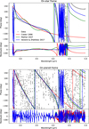 |
Fig. 2 Measured differential phase (grey dots) in two MATISSE frames, one on the star (top) and the other on the planet (bottom). Overlaid are the models presented in this work using the air refractive indices of Voronin & Zheltikov (2017) (blue), Mathar (2007) (green), and Ciddor (1996) (red). In the absence of chromatic or non-common path OPD, the differential phase should be zero on the star or an oscillation on the planet. |
3.2.2 Calibration and binning
Frames on the star and the planet are affected by telluric lines. In addition, the on-planet coherent fluxes are contaminated by the stellar halo leaking into the pinhole. To correct it, we used the on-star frames as a calibrator proxy for the on-planet frames. We divided the complex coherent flux of each on-planet frame by the mean coherent flux of the on-star frames in the next observation block (see Table 1). This removed most of the telluric lines and the high-order variations in the stellar contaminating spectrum, only leaving a low-order function created by the chromatic variation in the stellar speckle halo. This can be seen in the data in Fig. 3, in which the amplitudes of the planet-star modulations vary across wavelengths. This contamination will be modelled in the next section.
The MATISSE LM-band detector oversamples the spectral resolution by a factor of five in the medium-resolution mode (R = 500)6. In order to gain signal-to-noise (S/N) and prevent correlations between spectral pixels, while conserving the spectral resolution, we binned the coherent flux and their errors into blocks of 5 pixels.
4 Astrometry and spectrum extraction
The extraction of the planet’s astrometry and spectrum follows the outline of the method used by the ExoGRAVITY collaboration (see the appendices of GRAVITY Collaboration 2020; Nowak et al. 2020) with some modifications specific to MATISSE and its lack of absolute metrology. On each baseline, assuming the star and planet are point sources, we modelled the complex coherent fluxes obtained when MATISSE is centred on the planet (Fp) and on the star (F⋆) as follows:
![Mathematical equation: $\[F_p\left(\lambda, t_p, \boldsymbol{r}_p\right)=T\left(\lambda, t_p\right)\left[S_p(\lambda)+R\left(\lambda, t_p, \boldsymbol{r}_p\right) S_{\star}(\lambda) \mathrm{e}^{\mathrm{i} \frac{\mathrm{2} \pi \alpha u}{\lambda}}\right] \mathrm{e}^{\mathrm{i} \Phi\left(\lambda, t_p\right)},\]$](/articles/aa/full_html/2025/12/aa53323-24/aa53323-24-eq5.png) (5)
(5)
![Mathematical equation: $\[F_{\star}\left(\lambda, t_{\star}, \boldsymbol{r}_{\star}\right)=T\left(\lambda, t_{\star}\right) S_{\star}(\lambda) \mathrm{e}^{\mathrm{i} \Phi\left(\lambda, t_{\star}\right)},\]$](/articles/aa/full_html/2025/12/aa53323-24/aa53323-24-eq6.png) (6)
(6)
in which the p and ⋆ indices designate the on-planet and on-star frames, respectively. λ, t, and r are the wavelength, the observation time, and the pinhole location on sky; and T, Sp, and S⋆ are the telluric and instrumental transmission, the planet spectrum, and the stellar spectrum, respectively. R is the star-to-speckle contrast, i.e. the wavelength-dependent stellar point spread function (PSF) at the planet location, which depends on the seeing and AO correction. Together, RS⋆ thus models the speckle spectrum at the planet location. α is the (Δα, Δδ) angular offset vector of the planet from the star, and u is the (u, v) baseline vector of the observation. Finally, Φ is a phase component not originating in the targets, i.e. uncorrected atmospheric or instrumental phase components. Given the good correction of the chromatic dispersion and non-common path OPD obtained in Sect. 3.2.1, we assume in the following steps that this residual phase is negligible: Φ(λ) ≈ 0.
We use in our study the ratio between the on-planet and on-star coherent fluxes, ℱ:
![Mathematical equation: $\[\mathcal{F}=\frac{F_p\left(\lambda, t_p, \boldsymbol{r}_p\right)}{F_{\star}\left(\lambda, t_{\star}, \boldsymbol{r}_{\star}\right)} \approx \tau\left(\lambda, t_p, t_{\star}\right)\left[C(\lambda)+R\left(\lambda, t_p, \boldsymbol{r}_p\right) \mathrm{e}^{\mathrm{i} \frac{2 \pi \alpha u}{\lambda}}\right],\]$](/articles/aa/full_html/2025/12/aa53323-24/aa53323-24-eq7.png) (7)
(7)
in which C(λ) = Sp(λ)/S⋆(λ) is the planet-to-star contrast spectrum, and τ(λ, tp, t⋆) = T(λ, tp)/T(λ, t⋆). To calculate this ratio, the coherent flux, Fp, of each planet frame was divided by the average of the stellar coherent fluxes, F⋆, in the next stellar OB. We did not calibrate the telluric transmission with dedicated software such as Molecfit (Smette et al. 2015; Kausch et al. 2015). This would be possible on the on-star data but not on the on-planet data, which is too noisy for such an analysis. We instead relied on the small variations in airmass and water vapour between observation blocks (see Table 1), and assumed that the telluric transmission ratio between on-planet and on-star exposures can be modelled by a simple achromatic factor: τ(λ, tp, t⋆) = τ(tp, t⋆). Following GRAVITY’s two-step extraction procedure, we first extracted the astrometry and the starlight transmission function, and then the contrast spectrum.
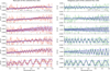 |
Fig. 3 Real (left) and imaginary (right) parts of the measured planet-to-star coherent flux ratio, ℱ, on the six UT baselines, during one 10 s frame. The error range is plotted in the background. The thick lines show the best-fit model as described in Sect. 4.1. It includes the star–planet modulation, the stellar speckle contamination (dashed blue curves), and the planet-to-star contrast assumption (dashed black curve). |
4.1 Astrometry and starlight contamination fitting
To first extract the astrometry, we need to assume a model Cmodel(λ) for the planet-to-star contrast spectrum. We used for this purpose the ratio between a model of stellar spectrum and a model of planetary spectrum. For the planet, we took a BT-Settl (Allard et al. 2013) sub-stellar template close to the known parameters (Teff = 1700 K, log g = 4.0, [M/H] = 0.0). For the star, we used a BT-NextGen (Allard et al. 2012) template interpolated with species7 (Stolker et al. 2020) at Teff = 7890 K and log g = 3.83 (Swastik et al. 2021), and scaled according to archival photometric fluxes from Tycho (Høg et al. 2000), 2MASS (Skrutskie et al. 2006), and Gaia (Gaia Collaboration 2023), as shown in Fig. 4. The fitted scale factor has an uncertainty of ~1.5% stemming from the photometric flux uncertainties. Each template was convolved at R = 500 and resampled on the MATISSE wavelength grid using spectres (Carnall 2017). The ratio was finally scaled according to the reported L′-band contrast (7.7 mag, Lagrange et al. 2009). Based on Eq. (7), our fit is now described by
![Mathematical equation: $\[\mathcal{F}_{\text {model }}(\lambda)=\mathcal{T}\left(t_p, t_{\star}\right) C_{\text {model }}(\lambda)+\mathcal{R}\left(\lambda, t_p, \boldsymbol{r}_p\right) \mathrm{e}^{\mathrm{i} \frac{\mathrm{2} \pi \alpha u}{\lambda}},\]$](/articles/aa/full_html/2025/12/aa53323-24/aa53323-24-eq8.png) (8)
(8)
where 𝒯(tp, t⋆) = γ τ(tp, t⋆) is the product of the telluric and instrumental transmission ratio, τ, with a factor, γ, reflecting possible inaccuracies in the scaling of the contrast template, and ℛ(λ, tp, rp) = τ(tp, t⋆) R(λ, tp, rp) is the product of τ with the stellar contamination R. Following the ExoGRAVITY method, we assume that the stellar contamination varies slowly with wavelength and therefore model ℛ with a low-order polynomial. The fit was performed baseline by baseline (b), frame by frame (tp), and for each point of a grid of tested planet offsets (Δα, Δδ). We minimized the least-square residuals of the real and imaginary parts of the coherent flux ratios (considered independent), using errors propagated from those provided by the MATISSE pipeline:
![Mathematical equation: $\[\begin{aligned}\chi^2\left(t_p, b, \Delta \alpha, \Delta \delta\right)= & \sum_\lambda \frac{\Re \mathrm{e}\left[\mathcal{F}(\lambda)-\mathcal{F}_{\text {model }}(\lambda)\right]^2}{\sigma_{\Re \mathrm{e}[\mathcal{F}(\lambda)]}^2} \\& +\sum_\lambda \frac{\mathfrak{I} \mathrm{m}\left[\mathcal{F}(\lambda)-\mathcal{F}_{\text {model }}(\lambda)\right]^2}{\sigma_{\Im \mathrm{m}[\mathcal{F}(\lambda)]}^2}.\end{aligned}\]$](/articles/aa/full_html/2025/12/aa53323-24/aa53323-24-eq9.png) (9)
(9)
For each of these iterations, we fitted the 𝒯 factor and the polynomial coefficients of ℛ. We tried to fit either the same or two different polynomial functions to the real and imaginary parts of the flux, and tried several polynomial orders. Overall, we found that fitting two different first-order polynomial functions for the real and imaginary parts is slightly favoured in terms of reduced chi-squared (![Mathematical equation: $\[\chi_{r}^{2}\]$](/articles/aa/full_html/2025/12/aa53323-24/aa53323-24-eq13.png) ). In total, we thus have five fitted parameters per fit: one for the transmission factor, 𝒯, and four for the two linear functions, ℛreal and ℛimag. We excluded from the fit the regions of strong telluric absorption below 2.87 μm and between 4.15 and 4.57 μm. We also excluded outliers deviating from the median coherent flux ratio by more than 3σ (computed from the median absolute deviation: σ = 1.4826 MAD) in L and M bands separately, amounting to 3–7% of the data. An example of match between the model and the data of a single frame is shown in Fig. 3.
). In total, we thus have five fitted parameters per fit: one for the transmission factor, 𝒯, and four for the two linear functions, ℛreal and ℛimag. We excluded from the fit the regions of strong telluric absorption below 2.87 μm and between 4.15 and 4.57 μm. We also excluded outliers deviating from the median coherent flux ratio by more than 3σ (computed from the median absolute deviation: σ = 1.4826 MAD) in L and M bands separately, amounting to 3–7% of the data. An example of match between the model and the data of a single frame is shown in Fig. 3.
With a ![Mathematical equation: $\[\chi_{r}^{2}\]$](/articles/aa/full_html/2025/12/aa53323-24/aa53323-24-eq14.png) value for each tested planet offset, we obtained one χ2 map per frame and baseline. We averaged all these maps together to get the total
value for each tested planet offset, we obtained one χ2 map per frame and baseline. We averaged all these maps together to get the total ![Mathematical equation: $\[\chi_{r}^{2}\]$](/articles/aa/full_html/2025/12/aa53323-24/aa53323-24-eq15.png) maps presented in Fig. 5. We ran this procedure on two different grids: a large one the size of MATISSE’s pinhole (130 mas) with a resolution of 1 mas, and a narrow one on a 20 × 20 mas square with a resolution of 0.1 mas. The grid is centred on the telescope pointing during the planet observation. We fitted an ellipse on the lowest peak of the narrow map to extract the best-fitting relative astrometry of β Pic
maps presented in Fig. 5. We ran this procedure on two different grids: a large one the size of MATISSE’s pinhole (130 mas) with a resolution of 1 mas, and a narrow one on a 20 × 20 mas square with a resolution of 0.1 mas. The grid is centred on the telescope pointing during the planet observation. We fitted an ellipse on the lowest peak of the narrow map to extract the best-fitting relative astrometry of β Pic ![Mathematical equation: $\[\mathrm{b}(\hat{\boldsymbol{\alpha}})\]$](/articles/aa/full_html/2025/12/aa53323-24/aa53323-24-eq16.png) , its associated errors, and the correlation coefficient, ρ, between Δα and Δδ measurements8. The values are reported in Table 2, along with the predictions of the orbital fit of Lacour et al. (2021) based on GRAVITY, GPI, and SPHERE data, computed with whereistheplanet at the same epoch as the MATISSE observations.
, its associated errors, and the correlation coefficient, ρ, between Δα and Δδ measurements8. The values are reported in Table 2, along with the predictions of the orbital fit of Lacour et al. (2021) based on GRAVITY, GPI, and SPHERE data, computed with whereistheplanet at the same epoch as the MATISSE observations.
The orbital fitting prediction is located 3.38 mas (~2σ) away from our MATISSE astrometry. The GRAVITY measurements it is based on are obtained by averaging the best-fit astrometries per frame or group of frames, which provides precisions of ~0.1 mas, an order of magnitude below the size of individual peaks in the χ2 maps. This method requires a consistent peak pattern between maps, which we do not get at the moment with MATISSE. We instead rely on the average of all χ2 maps, and are thus limited to a precision of a few milliarcseconds equivalent to the VLTI angular resolution. The stability of the GRAVITY astrometry stems from its internal metrology system (GRAVITY Collaboration 2017), which enables the phases measured on the planet to be anchored to the phases measured on the star, and correcting non-common path aberrations between fringe tracker and science combiner. MATISSE does not have such metrology, and is thus affected by time variations in residual non-common path aberrations between the star and planet pointings. In Figure B.3 we show the OPD drift measured on MATISSE, exhibiting the differential drift between GRA4MAT (fringe tracker) and MATISSE (science instrument). It currently is of the order of one wavelength over one hour. This drift may be reduced to sub-wavelength accuracy by adopting a different observing strategy in the future. To alleviate this issue for the moment, the data reduction is based on self-referenced phases (see Sect. 3.2.1), resulting in an additional astrometric noise of the order of about λ/B, with B the baseline length.
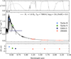 |
Fig. 4 Scaling of the BT-Nextgen stellar model (Teff = 7890 K, log g = 3.83, [Fe/H] = 0.0) with species using Tycho, Gaia, and 2MASS photometry of β Pictoris. The bottom panel shows the residuals of the fit. |
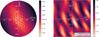 |
Fig. 5 Detection maps of β Pic b with MATISSE. The maps show the reduced χ2 values after fitting the stellar contamination for each tested planet astrometry (Δα, Δδ) in the grid. The grids are centred on MATISSE’s pointing during the planet observations. The left map is the size of the pinhole (1.5λ/D at 3.5 μm) and has a resolution of 1 mas. The right map was generated at higher resolution (0.1 mas) on a smaller 20 × 20 mas grid. The most likely astrometry from the MATISSE observations is shown as a blue ellipse, found by fitting a 2D Gaussian curve on the lowest |
![Mathematical equation: $\[\chi_{r}^{2}\]$](/articles/aa/full_html/2025/12/aa53323-24/aa53323-24-eq10.png)
![Mathematical equation: $\[\chi_{r}^{2}\]$](/articles/aa/full_html/2025/12/aa53323-24/aa53323-24-eq11.png)
![Mathematical equation: $\[\chi_{r}^{2}\]$](/articles/aa/full_html/2025/12/aa53323-24/aa53323-24-eq12.png)
Relative astrometry of β Pic b found in our analysis, and predictions from the orbital fit of Lacour et al. (2021) retrieved with whereistheplanet.
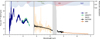 |
Fig. 6 Spectrum of β Pic b with MATISSE (black, this work) compared to other instruments: NACO (yellow, new data), GPI (blue, Chilcote et al. 2017), GRAVITY (green, new data) and MIRI (red, Worthen et al. 2024). Only the slope of the NACO spectrum can be compared to MATISSE as the absolute level was scaled manually. MATISSE data with a S/N < 5, located in strong telluric bands and not used in this work, are shown in grey. The absorption curves of H2O, CO, and CH4, calculated from the best-fitting Exo-REM model presented in Sect. 5, are plotted at the top to visualize their impact on the spectrum. H2O and CO leaves a visible pattern, but not CH4, likely because it is dominated by H2O absorption or buried in noise. |
4.2 Spectrum extraction
Once we had the best-fitting astrometry, ![Mathematical equation: $\[\hat{\boldsymbol{\alpha}}\]$](/articles/aa/full_html/2025/12/aa53323-24/aa53323-24-eq17.png) , we extracted the associated fit of the stellar contamination function,
, we extracted the associated fit of the stellar contamination function, ![Mathematical equation: $\[\hat{\mathcal{R}}\]$](/articles/aa/full_html/2025/12/aa53323-24/aa53323-24-eq18.png) , at this position, for each frame and each baseline. Following Eq. (7), we then estimated the contrast spectrum as follows:
, at this position, for each frame and each baseline. Following Eq. (7), we then estimated the contrast spectrum as follows:
![Mathematical equation: $\[\hat{C}\left(\lambda, t_p, b\right)=\Re \mathfrak{e}\left[\frac{\mathcal{F}\left(\lambda, t_p, b\right)}{\tau\left(\lambda, t_p, t_{\star}\right)}-\hat{\mathcal{R}}\left(\lambda, t_p, b, \hat{\boldsymbol{\alpha}}\right) \mathrm{e}^{\mathrm{i} \frac{2 \pi \hat{\alpha} u}{\lambda}}\right].\]$](/articles/aa/full_html/2025/12/aa53323-24/aa53323-24-eq19.png) (10)
(10)
We neglected the transmission ratio, τ(tp, t⋆), as 𝒯(tp, t⋆) was consistently fitted close to one in the previous section. With this method, we obtained 1308 estimates of the contrast spectrum (218 frames × 6 baselines). Before averaging them, we first excluded points outlying by more than 3σ (estimated from the median absolute deviation) from the median at each wavelength, which removed ~1% of points inside the L and M bands. We finally computed the mean and the covariance of the mean to get our final estimate of the contrast spectrum and its errors. The covariance matrix was computed by considering the 1308 contrast spectra as samples and the wavelengths as variables.
In order to get the planet spectrum, we have to multiply the contrast by a stellar spectrum. We initially used a β Pic spectrum from the Infrared Space Observatory (Pantin et al. 1999) at R = 2000, but the high-resolution archival data is affected by calibration issues in the M band, and it does not fully cover the K-band wavelengths of GRAVITY which we will use in the modelling. For these reasons, we instead use the same BT-NextGen stellar template as computed in Sect. 4.1. The resulting planet spectrum is shown in Fig. 6, covering the full L band and the blue side of the M band. We added several other spectra of β Pic b from different instruments: Gemini/GPI (Chilcote et al. 2017), JWST/MIRI (Worthen et al. 2024), and two original spectra from VLTI/GRAVITY (S. Lacour, private communication) and VLT/NACO (M. Bonnefoy, private communication). The GRAVITY spectrum is a weighted mean of several epochs since the first publication in GRAVITY Collaboration (2020). We used the contrast spectrum and scaled it with the same stellar model as the MATISSE data. The NACO spectrum was obtained in 2011. The acquisition and reduction of these new spectra are described in Appendix C. We note that the NACO spectrum was scaled manually, so only its slope can be compared to the MATISSE spectrum.
The LM-band MATISSE spectrum of β Pic b seems to be affected by broad absorption features. To verify how the main absorbers, H2O, CO, and possibly CH4, impact the SED, we calculated their individual absorption curves as in Palma-Bifani et al. (2024). These curves were obtained from the best-fitting Exo-REM model. This model and the method to generate molecular absorption curves are presented in Sect. 5. The absorption curves are shown at the top of Fig. 6. They show that the L band (2.8–4.2 μm) is shaped by H2O, while the M-band subregion observed by MATISSE (4.5–5 μm) is shaped primarily by CO, and secondarily by H2O. The CH4 band at 3.3 μm does not seem visible, either because H2O absorption dominates it or because it is buried in noise.
Some small-amplitude periodic features also appear in the spectrum, in particular between 3 and 3.5 μm. They seem associated with off-diagonal periodic correlations in the covariance matrix of the spectrum, presented in Fig. 7. This matrix was built by scaling the contrast covariance with the stellar model: σSp (λi, λj) = S⋆(λi) S⋆(λj) σC(λi, λj). We believe these periodic correlations come from the instrument and/or the processing rather than the source itself. Their frequency seems indeed related to the star–planet modulations of the coherent flux, i.e. the phasor term in Eq. (7), whose frequency also decreases with wavelength (∝ 1/λ). We note that even if we cannot distinguish these residuals from spectral features, their presence in the covariance matrix should prevent them from biasing the atmospheric parameters fitted through forward modelling (Sect. 5).
These periodic residuals could come from an imperfect fit of the stellar speckle function (ℛ in Eq. (8)). The planet-to-speckle contrast in our observations is close to one, while it was 3–5% in the GRAVITY observations (GRAVITY Collaboration 2020). This is expected from several factors: the 4× brighter intrinsic planet-to-star contrast in L than in K, the larger separation at the time of our observation (534 vs 144 mas), and the larger spatial filter used in MATISSE (135 vs 60 mas). A planet-to-speckle contrast of order unity means that C (the planet-to-star contrast) and ℛ (the star-to-speckle contrast) are on the same order of magnitude, and might thus be more correlated in our fit than they did in GRAVITY observations. To ensure that the assumed contrast model in Sect. 4.1 does not influence the shape of the final contrast spectrum, we ran the same fit using a flat contrast model at 7 × 10⁻⁴. The contrast spectrum extracted with this simplistic assumption has the same slope and absolute level as the one obtained with the realistic assumption, with only the oscillations below 3.5 μm varying slightly. As is seen in Fig. 3, the large bandwidth of MATISSE provides many periods of the star–planet modulations, likely enabling a good fit of the stellar speckle contamination ℛ without large correlation with the chosen contrast model. Nonetheless, a simultaneous fit of C and ℛ is preferable to improve accuracy. Since C(λ) is defined for hundreds of wavelengths, this fit can only be performed by fitting simultaneously on a large number of DITs, as is done for GRAVITY observations. This supposes that the coherent fluxes of all DITs are cophased. We cannot assume this at the moment for MATISSE due to its lack of metrology, which is why we extracted our spectrum DIT by DIT instead of fitting it simultaneously on all the data. Methods to co-phase MATISSE DITs together are being investigated and will be the subject of a future publication.
The relative errors shown on the MATISSE spectrum were extracted from the covariance diagonal. They range from 1% of the flux in the middle of the L band to ~5% in the M band. The absolute MATISSE flux matches well with the MIRI spectrum in their overlapping region, but seems to have a mismatch of ~10% with the GRAVITY spectrum, as well as with previous photometric measurements. We computed an estimated L′ magnitude by convolving this spectrum with the Paranal/NACO L′ filter available on the SVO Filter Profile Service (Rodrigo et al. 2012; Rodrigo & Solano 2020). We find ![Mathematical equation: $\[L_{\text {MATISSE}}^{\prime}=10.970 \pm 0.005\]$](/articles/aa/full_html/2025/12/aa53323-24/aa53323-24-eq20.png) , which is 23.5% higher but within the error bars of the measurement of Lagrange et al. (2009) (11.2 ± 0.3 mag). Flux discrepancies have been noted in many studies combining different instrument spectra, and can be seen here as well between GPI and GRAVITY. Several reasons may explain them in our case.
, which is 23.5% higher but within the error bars of the measurement of Lagrange et al. (2009) (11.2 ± 0.3 mag). Flux discrepancies have been noted in many studies combining different instrument spectra, and can be seen here as well between GPI and GRAVITY. Several reasons may explain them in our case.
Firstly, the absolute precision is limited by the 1.5% precision on the scaling of the stellar model (see Sect. 4.1), but this cannot explain the mismatch with GRAVITY as the same model was used. Secondly, the star is partly resolved by MATISSE. Priolet et al. (2025) find a visibility decrease of ~5% on the longest baselines on β Pic, interpreted as the resolved star surrounded by an inner disc. This means that the stellar coherent flux is affected by this visibility and is lower than the stellar spectrum. As a result, the planet spectrum is overestimated if we do not take into account the stellar visibility when we multiply the contrast by the stellar template. The inner disc may also add emission in the stellar spectrum, which is not taken into account in the stellar template. The β Pic interferometric data of Priolet et al. (2025) could be used to estimate and correct these effects. Another factor may be the loss of coherent flux induced by phase jittering during a science integration (Colavita 1999; Tatulli et al. 2007). It is taken into account in the GRAVITY pipeline through the calculation of the so-called ‘vFactor’ based on the high-frequency fringe tracker data9. We implemented it in our MATISSE processing by using the simultaneous GRAVITY fringe tracking data, but it results in no substantial difference in the final planet spectrum, possibly because of close vFactors in the on-planet and on-star frames cancelling each other when we take the ratio. Another final possibility is a phase jitter not seen by the fringe tracker when recording on the planet in the narrow VLTI field.
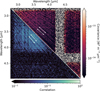 |
Fig. 7 Covariance (upper right triangle) and correlation (lower left triangle) matrices of the MATISSE spectrum of β Pic b. In order to highlight the off-diagonal correlations in the L band, the covariance values are clipped between 3 × 10⁻³⁵ and 3 × 10⁻³³ W2 m−4 μm−2 and the correlation values between 0.01 and 1. Two lines of off-diagonal correlations are further highlighted with arrows for readability. |
5 Forward modelling
To check the physical consistency of the spectrum obtained with MATISSE, we compared it along the new GRAVITY spectrum to the same grid of Exo-REM model spectra (Baudino et al. 2015; Charnay et al. 2018; Blain et al. 2021) that was used in GRAVITY Collaboration (2020). Exo-REM is a self-consistent atmospheric model assuming radiative-convective equilibrium, incorporating simple cloud microphysics that was shown to well reproduce the L-T transition of brown dwarfs and giant planets. For more advanced modelling, we refer to the study of Ravet et al. (2025) which uses all the available archival data of β Pic b (including our MATISSE spectrum) and four different grids of models (Exo-REM, ATMO, SONORA, BT-Settl).
To fit the models, we used the Bayesian inference ForMoSA10 code (Petrus et al. 2021, 2023; Palma-Bifani et al. 2023), which evaluates posterior density functions on each free parameter of the model grid based on a nested sampling algorithm. The code performs an N-dimensional linear interpolation of the precomputed grids of models between the grid nodes on the fly. The Exo-REM grid has four dimensions, corresponding to the set of free parameters of the self-consistent Exo-REM models: effective temperature (Teff), surface gravity (log g), carbon-to-oxygen ratio (C/O), and metallicity ([M/H]). In addition to the grid parameters, ForMoSA fits the companion bolometric luminosity (or radius or distance if one of these is provided as fixed prior), radial velocity, and rotational velocity. Finally, it can fit scale factors (α) to different datasets in order to account for flux calibration issues.
β Pic b is part of a limited sample of directly imaged planets with a dynamical mass constrained from orbital fits of astrometric measurements (see Sect. 1). To take advantage of this knowledge, we implemented in ForMoSA the possibility to fit and use the mass as a prior. This replaces in practice the planet radius, which is now set by the sampled mass and surface gravity through the surface gravity definition:
![Mathematical equation: $\[R=\sqrt{\frac{G M}{10^{\log g}}}.\]$](/articles/aa/full_html/2025/12/aa53323-24/aa53323-24-eq31.png) (11)
(11)
This in turn sets the bolometric luminosity of the model via the dilution factor (R/d)2 applied to the synthetic spectra to convert them to apparent fluxes. The priors of our fits are listed in Table 3. The mass and distance are set with Gaussian priors based on stellar and planetary astrometry from Nielsen et al. (2020) and GRAVITY Collaboration (2020), respectively. All the other parameters are set with uniform priors. The radial and rotational velocities are not fitted, as their effects are negligible at R = 500.
We fitted models successively on MATISSE only, GRAVITY only, and on GRAVITY and MATISSE spectra together, using 500 live points, and taking into account their covariance matrices. For the joint GRAVITY+MATISSE fits, we perform two fits in which we use a scale factor either on GRAVITY or on MATISSE, to account for the discrepancy between spectra noted in Sect. 4. We show in Fig. 8 the best-fit Exo-REM models together with the MATISSE and GRAVITY data. Our estimates on each parameter and their fitting errors (inferred from the 68% confidence intervals on the posteriors) are reported in Table 3. We caution that the uncertainties are only a projection of the observational errors on the model predictions and do not account for systematic deviations of the models that certainly dominate here. A more systematic study of these deviations is explored in Ravet et al. (2025) based on the full collection of spectrophotometry obtained on β Pic b thus far.
The best models for the joint GRAVITY+MATISSE fits are found for Teff = 1529 ± 3 K, log g = 3.83 ± 0.04, [M/H] = 0.30 ± 0.03, and C/O = 0.539 ± 0.003. Scaling either the GRAVITY or MATISSE spectra only changes the fitted mass, which sets the radius and thus the absolute flux level in conjunction with log g. We find masses of 10.5 ± 0.7 and 11.8 ± 0.9 MJup when scaling MATISSE or GRAVITY, respectively. Figure 9 shows the corner plot of the best-fit model (GRAVITY+MATISSE fixed). We finally note that fitting only the GRAVITY data provides posteriors that are very close to the joint fits.
From the best-fitting model, we generated the absorption curves of individual molecules (H2O, CO, and CH4) plotted in Fig. 6. These curves are built in the same way as full Exo-REM spectral models, but only including one molecule at a time. We consider collision-induced absorption (CIA) of H2–H2 and H2-He, Rayleigh scattering, and the cross-section of each molecule. We used the P-T profile and volume-mixing ratios of the best-fitting model, and generated absorption curves for each molecule with the opacity library Exo_k (Leconte 2021). We finally normalized each molecular curve by the CIA-only spectrum for visualization.
Best-fit parameters found with ForMoSA on the Exo-REM model grid.
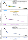 |
Fig. 8 GRAVITY and MATISSE spectra of β Pic b with the best-fit Exo-REM models. The top plot shows the best fits on GRAVITY only, MATISSE only, and GRAVITY+MATISSE, when no scaling is applied on the spectra. The two other plots show the best fits on GRAVITY+MATISSE when a scale factor is applied either on MATISSE (middle) or on GRAVITY (bottom). |
6 Discussion
6.1 Solar C/O
We find C/O ratios compatible with or above solar abundances, varying from 0.524 ± 0.004 (GRAVITY data alone) up to 0.775 ± 0.002 (MATISSE data alone). We adopt here the value of 0.539 ± 0.003 found when jointly fitting both datasets. We note that the errors we get from these fits are an order of magnitude smaller than the errors on the C/O of β Pic b obtained by GRAVITY Collaboration (2020). These errors are likely underestimated for the reasons mentioned in Sect. 5.
This new solar C/O is higher than the subsolar values of 0.43 ± 0.05 and 0.41 ± 0.04 found by GRAVITY Collaboration (2020) and Landman et al. (2024), respectively. The former was obtained by forward modelling (with Exo-REM) and atmospheric retrieval (with petitRADTRANS, Mollière et al. 2020) of JHK-band GRAVITY and GPI spectra. The latter was obtained by petitRADTRANS atmospheric retrieval of a K-band high-resolution (R = 100 000) CRIRES spectrum. The solar C/O is, however, in line with the value of 0.551 ± 0.002 found by Kiefer et al. (2024) with molecular mapping of SINFONI data. A high-resolution K-band survey with KPIC also found solar C/O for eight young sub-stellar companions (Xuan et al. 2024), although at larger orbital separations of 50–360 au, which might not be directly comparable with β Pic b at 8 au.
We note that fitting only the new GRAVITY spectrum also favours a solar C/O. This solar value is within ~2σ of the value of GRAVITY Collaboration (2020). This difference could be arising from the higher quality of the new spectrum, based on several more epochs of GRAVITY observations. This higher quality seems to be reflected in the better fit obtained on GRAVITY in this work using the same Exo-REM grid in both studies. The addition of MATISSE data also brings tighter constraints on the C/O thanks to the presence of broad H2O and CO absorption features.
To examine this issue further, we fitted Exo-REM models with low (0.430 ± 0.001) and high (0.650 ± 0.001) C/O Gaussian priors to our GRAVITY+MATISSE datasets. All the other parameters keep the uniform priors used in Sect. 5, and the scale factor is applied only on GRAVITY. The posteriors of these new fits are listed in Table 4, and the models are plotted in Fig. 10. The solar C/O remains favoured over the low and high C/O both for GRAVITY (![Mathematical equation: $\[\chi_{r}^{2}\]$](/articles/aa/full_html/2025/12/aa53323-24/aa53323-24-eq36.png) = 2.38 over 2.75 and 2.98, respectively) and MATISSE (
= 2.38 over 2.75 and 2.98, respectively) and MATISSE (![Mathematical equation: $\[\chi_{r}^{2}\]$](/articles/aa/full_html/2025/12/aa53323-24/aa53323-24-eq37.png) = 4.28 over 5.07 and 4.45, respectively). Calculating the likelihood ratio as ΔL = Δχ2/2, this means that the solar C/O model is more likely than the low and high C/O models by factors of ~43 and 67 for GRAVITY, respectively, and ~91 and 20 for MATISSE, respectively.
= 4.28 over 5.07 and 4.45, respectively). Calculating the likelihood ratio as ΔL = Δχ2/2, this means that the solar C/O model is more likely than the low and high C/O models by factors of ~43 and 67 for GRAVITY, respectively, and ~91 and 20 for MATISSE, respectively.
GRAVITY Collaboration (2020) modelled the variation in C/O as function of the accreted mass of solid material, assuming a solar C/O value for the star and either a gravitational collapse or a core accretion scenario. A low C/O value makes the gravitational collapse scenario unlikely within the effective time available for efficient accretion of solid planetesimals during the pre-collapse stage, and favours rather a core accretion scenario between the CO2 and H2O icelines. Following their Fig. 6 and 7, if the planetary C/O is solar as found in our study, this would place gravitational collapse back in the possible scenarios with core accretion. Kiefer et al. (2024) notes that a solar C/O could be reached by gravitational instability anywhere in the disc, or by core accretion close to the H2O ice line with a moderate planetesimal accretion followed by an outward migration. They consider the latter scenario more likely considering that core accretion is preferred for most compact planetary systems with terrestrial planets, and that the β Pic system has at least two planets within 8 au and small km-sized icy bodies (Lecavelier des Etangs et al. 2022). The planetesimal accretion is corroborated by the enhanced metallicity we retrieve ([M/H] = 0.30 ± 0.03).
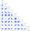 |
Fig. 9 Corner plot of the joint fit of GRAVITY (freely scaled) and MATISSE (fixed) spectra, using ForMoSA and the Exo-REM model grid. |
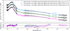 |
Fig. 10 Fit of Exo-REM models using low (pink) and high (blue) C/O priors, compared to the free uniform C/O prior (green) already presented in Fig. 8. |
Best-fit parameters using low (0.430 ± 0.001) and high (0.650 ± 0.001) Gaussian C/O priors, all other priors remaining unchanged.
6.2 Other atmospheric parameters
The Teff (1529 K) and log g (3.84) of our best model are similar to those obtained by previous forward modelling studies that used Exo-REM, while the radius R (~2 RJup) is similar or slightly higher: Baudino et al. (2015) (on photometry: 1550 K, 3.5, 1.76 RJup), GRAVITY Collaboration (2020) (on GRAVITY and GPI spectra: 1590 K, 4.0, 1.79 RJup), Worthen et al. (2024) (on MIRI, GPI, GRAVITY spectra + photometry: 1471 K, 3.71, 1.97 RJup). Studies based on forward modelling of ATMO (Phillips et al. 2020) and DRIFT-PHOENIX (Helling et al. 2008) grids, or on radiative transfer retrieval (petitRADTRANS, Mollière et al. 2019) tend, however, to find temperatures > 1700 K and smaller radii of ~1.4 RJup (Chilcote et al. 2017; GRAVITY Collaboration 2020; Worthen et al. 2024). The modelling study including the most data to this day (Ravet et al. 2025) found close results to ours (Teff ~ 1500–1600 K, log g ~ 4.0–4.5) both using Exo-REM and SONORA, while finding high-Teff (>1800 K) and low-log g (<3.5) solutions using ATMO and BT-Settl. We refer the reader to their paper for a more comprehensive modelling of the SED of β Pic b, and a discussion of the differences between grids of models.
The fitted mass of our best model shifted from an initial prior of 12.7 ± 2.2 MJup (from the dynamical mass of GRAVITY Collaboration 2020) to posteriors of 10.5 ± 0.7 (GRAVITY fixed) or 11.8 ± 0.9 MJup (MATISSE fixed). These posteriors are well in agreement with the latest dynamical mass estimates using GRAVITY, radial velocity and imaging: ![Mathematical equation: $\[9.3_{-2.6}^{+2.5}\]$](/articles/aa/full_html/2025/12/aa53323-24/aa53323-24-eq38.png) (Brandt et al. 2021) and
(Brandt et al. 2021) and ![Mathematical equation: $\[11.90_{-3.04}^{+2.93}\]$](/articles/aa/full_html/2025/12/aa53323-24/aa53323-24-eq39.png) MJup (Lacour et al. 2021). If we can be relatively confident about the mass, the parameters correlated to it, log g and R (the latest being derived from the two others) are off compared to what is expected from evolutionary models. Based on an estimated age of 24 ± 3 Myr and a bolometric luminosity log L/L⊙ = −3.76 ± 0.02, and comparing them to Baraffe et al. (2003) hot-start evolutionary models, Chilcote et al. (2017) found expected log g and R of 4.18 ± 0.01 dex and 1.46 ± 0.01 RJup, respectively. The reasons for this discrepancy could be both on the model and data sides. On the model side, inconsistencies have already been noted between evolutionary and atmospheric models, as explained in Carter et al. (2023). Additionally, model uncertainties are not estimated (both for evolutionary models and spectral grids), which would result in higher uncertainties to the fitted parameters if provided. On the data side, as explained in Sect. 4.2, the flux calibration of our GRAVITY and MATISSE spectra could be too high, either from overestimated stellar flux or interferometric stellar visibility (if the star is actually resolved). The stellar visibilities measured by Priolet et al. (2025) could help us to derive a more accurate flux calibration.
MJup (Lacour et al. 2021). If we can be relatively confident about the mass, the parameters correlated to it, log g and R (the latest being derived from the two others) are off compared to what is expected from evolutionary models. Based on an estimated age of 24 ± 3 Myr and a bolometric luminosity log L/L⊙ = −3.76 ± 0.02, and comparing them to Baraffe et al. (2003) hot-start evolutionary models, Chilcote et al. (2017) found expected log g and R of 4.18 ± 0.01 dex and 1.46 ± 0.01 RJup, respectively. The reasons for this discrepancy could be both on the model and data sides. On the model side, inconsistencies have already been noted between evolutionary and atmospheric models, as explained in Carter et al. (2023). Additionally, model uncertainties are not estimated (both for evolutionary models and spectral grids), which would result in higher uncertainties to the fitted parameters if provided. On the data side, as explained in Sect. 4.2, the flux calibration of our GRAVITY and MATISSE spectra could be too high, either from overestimated stellar flux or interferometric stellar visibility (if the star is actually resolved). The stellar visibilities measured by Priolet et al. (2025) could help us to derive a more accurate flux calibration.
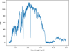 |
Fig. 11 Signal-to-noise ratio calculated on the MATISSE contrast spectrum of β Pic b. |
6.3 The potential of LM-band exoplanet interferometry
We obtain a high median S/N of ~80 in L band, with maximal values peaking at ~120 around 3.5 μm, as shown in Fig. 11. With this high quality, we expect to be able to characterize fainter and closer-in sub-stellar companions in the future. Separation ranges and L-band fluxes of a sample of planets and brown dwarfs are reported in Fig. 12.
The spectrum of β Pic b in L and M bands presents broad absorption bands of CO and H2O that can be used to constrain its atmosphere, but it does not show narrow absorption bands or lines, due to its relatively high temperature of ~1500 K. Colder giant planets and brown dwarfs at the L-T transition or below are expected to have deeper absorption bands, including narrow bands of CH4 at 3.3 μm (seen in early-L to T-type brown dwarfs and young planet analogues, Sorahana & Yamamura 2012; Miles et al. 2023) and CO2 at 4.2 μm (not accessible from the ground). At medium and high resolution (R > 500), these absorption bands and some spectral lines are resolved. Separating them from each other helps them to be matched to line lists and makes the estimation of molecular abundances easier. These abundances are tracers of the planet birthplace and formation scenario, through C/O and other elemental ratios (Öberg et al. 2011). These abundances can also constrain the disequilibrium chemistry at play in these atmospheres, which becomes particularly important for giant planets below the L–T transition (<1200 K, Charnay et al. 2018; Phillips et al. 2020).
Interferometry is so far the only technique that has obtained medium-resolution spectra of directly detected exoplanets at separations shorter than 0.2″. Like GRAVITY, MATISSE has the potential to observe companions at these separations and provide a complementarity to the JWST, which is not equipped with coronagraphy on its spectroscopic modes and may thus have difficulty getting spectra at these close separations. Ruffio et al. (2024) demonstrated a sensitivity of 3 × 10⁻⁵ at 0.3″ (only 3 spaxels away from the star) for JWST/NIRSpec, but contrast limits below this separation are still unknown, as well as the ability to retain the continuum of the planetary spectrum. For now, companions characterized by interferometry have come mainly from the sample of a few dozen sub-stellar companions discovered by direct imaging. A few interferometric targets have been detected first by radial velocity (Nowak et al. 2020; Hinkley et al. 2023) and astrometric surveys (Gaia DR3, Pourré et al. 2024; Winterhalder et al. 2024). With the fourth Gaia Data Release in 2026, based on more than five years of data, potentially several tens of thousands of long-period Jupiter-mass planets are expected to be discovered (Perryman et al. 2014). Among them, several dozens could be accessible to interferometry (GRAVITY+ Collaboration 2022). Obtaining dynamical masses and KLM fluxes on an order of magnitude more planets with GRAVITY and MATISSE could break the current degeneracy between mass, age, and luminosity in planetary evolutionary models, which results from poor constraints on the post-formation luminosity of giant planets (Mordasini et al. 2017). This will be extremely useful for exoplanet imaging as it relies on a planet’s luminosity to estimate its mass through evolutionary models. This should thus improve the precision on the masses of directly imaged planets, which are often poorly constrained at the moment. It will also better constrain the accretion mechanism in forming planets, which is responsible for the heat accumulated by a planet at the end of its formation.
Finally, the new AO system of the VLTI provided by the GRAVITY+ project, GPAO (Millour et al. 2024), will improve the performances of MATISSE even further in the near future. Switching from MACAO to GPAO, the Strehl ratio is expected to increase from 70% to 90% in L band, which will increase the planet flux injection into the spatial filter of MATISSE by 30%. This better AO correction will in addition reduce the stellar speckle background by a factor of 2 to 5 within the AO correction radius. These two improvements should lead to an increase in planetary S/N by a factor ranging from 1.1× (for planet-to-speckle contrasts ≫ 0.5) to 1.8–2.9x (for planet-to-speckle contrasts ≪0.5, depending on the separation) with GPAO compared to MACAO. These two improvements should lead to a 1.2–2.9× increase in the S/N on the planet with GPAO compared to MACAO, depending on the contrast and separation. Furthermore, the frequency of fringe jumps, which was already well reduced by the latest fringe tracker update (Nowak et al. 2024; Woillez et al. 2024), will decrease even more as result of the higher AO stability, increasing the quality of the MATISSE data. In addition, a dark hole observing strategy (an active speckle suppression technique, Malbet et al. 1995) is being developed on GRAVITY (Pourré et al. 2022). Using the new GPAO system, it could bring the GRAVITY detection limits from a current contrast limit of 4 × 10⁻⁵ at 75 mas down to 3 × 10⁻⁶ at 60 mas (Pourré et al. 2024). A similar strategy could be implemented on MATISSE to reach planets at higher contrasts and closer separations.
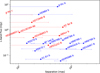 |
Fig. 12 Angular separations and L-band fluxes of a sample of exoplanets and brown dwarfs. Fluxes are either directly taken from the literature (blue points) or computed with ATMO and/or ExoREM models using atmospheric parameters fitted in the literature (red points). Minimal and maximal separations are represented as segments, while the current position of the planet is marked with an asterisk (except for β Pic c and HD 206893 c that are currently well below the MATISSE inner working angle). |
7 Conclusions
We observed an exoplanet for the first time with MATISSE using the newly offered GRA4MAT narrow off-axis mode. We developed a new method of correcting chromatic dispersion and non-common path features in the fringe phase. After extraction, we obtained the spectrum of β Pictoris b in the L and M bands at a spectral resolution of 500, showing broad absorption features of H2O and CO. We used the ForMoSA nested sampling tool and the Exo-REM grid to model the MATISSE spectrum jointly with a new GRAVITY spectrum stacking several years of observations. By imposing a mass prior based on the dynamical mass of β Pic b, we found a best model at Teff = 1529 ± 3 K, log g = 3.83 ± 0.04, [M/H] = 0.30 ± 0.03, and C/O = 0.539 ± 0.003. This solar C/O value was found both on the fits using only the new GRAVITY spectrum, and the ones using GRAVITY and MATISSE jointly. It is higher than the value found by GRAVITY Collaboration (2020) but in line with Kiefer et al. (2024). This solar C/O indicates that gravitational collapse is not excluded as a formation scenario for β Pic b, although core accretion might still remain favoured by other characteristics of the β Pic system.
The high S/N observed in our spectrum (median of 80 per spectral channel in the L band, with values as high as 120 at 3.5 μm) with only 36 min of integration on the planet indicates that fainter and closer-in companions should be accessible to MATISSE, which opens exciting perspectives for this observing technique and for mid-infrared spectroscopy. MATISSE should be able to complement JWST at short separations at which it cannot obtain spectra due to the absence of coronagraphs on its spectroscopic modes. This new window onto exoplanets comes at an exciting time when both the instrument capability and the exoplanet sample should extend in the near future. The new VLTI AO system, GPAO, has been commissioned since the end of 2024 and is already providing much higher performances than MACAO, thus injecting more planetary flux and less stellar contamination into the VLTI instruments. Finally, in 2026, Gaia DR4 is expected to bring potentially thousands of new exoplanet detections, of which dozens should be accessible to GRAVITY and MATISSE. By providing dynamical mass and KLM-band luminosity measurements on these Gaia companions, future large programs with GRAVITY and MATISSE have the potential to break the current mass-age-luminosity degeneracy in planetary evolutionary models. This will prove extremely useful for future observations with Extremely Large Telescope (ELT) instruments (HARMONI, Thatte et al. 2021; Houllé et al. 2021; METIS, Brandl et al. 2021; Bowens et al. 2021), which will require precise mass estimates to properly interpret their exquisite high-resolution spectroscopic data.
Acknowledgements
We thank the referee and the editor for their helpful comments. This work was supported by the French Agence Nationale de la Recherche (ANR), under grants ANR-21-CE31-0017 (EXOVLTI) and ANR-21-CE31-0018 (MASSIF). M. Bonnefoy acknowledges support in France from the French National Research Agency (ANR) through grants ANR-20-CE31-0012 and ANR-23-CE31-0006. This project has received funding from the European Research Council (ERC) under the European Union’s Horizon 2020 research and innovation programme (COBREX; grant agreement 885593). J. Varga is funded from the Hungarian NKFIH OTKA project nos. K-132406 and K-147380, and acknowledges support from the Fizeau exchange visitors program. J. J. Wang is supported by NASA XRP Grant 80NSSC23K0280. The research leading to these results has received funding from the European Union’s Horizon 2020 research and innovation programme under Grant Agreement 101004719 (ORP). This research has made use of the Jean-Marie Mariotti Center Aspro service11, and of the SVO Filter Profile Service “Carlos Rodrigo”, funded by MCIN/AEI/10.13039/501100011033/ through grant PID2020-112949GB-I00.
References
- Allard, F., Homeier, D., & Freytag, B. 2012, Philos. Trans. Roy. Soc. Lond. A, 370, 2765 [NASA ADS] [Google Scholar]
- Allard, F., Homeier, D., Freytag, B., Schaffenberger, W., & Rajpurohit, A. S. 2013, Mem. Soc. Astron. Ital. Suppl., 24, 128 [Google Scholar]
- Argyriou, I., Glasse, A., Law, D. R., et al. 2023, A&A, 675, A111 [NASA ADS] [CrossRef] [EDP Sciences] [Google Scholar]
- Baraffe, I., Chabrier, G., Barman, T. S., Allard, F., & Hauschildt, P. H. 2003, A&A, 402, 701 [NASA ADS] [CrossRef] [EDP Sciences] [Google Scholar]
- Baudino, J. L., Bézard, B., Boccaletti, A., et al. 2015, A&A, 582, A83 [NASA ADS] [CrossRef] [EDP Sciences] [Google Scholar]
- Beuzit, J. L., Vigan, A., Mouillet, D., et al. 2019, A&A, 631, A155 [NASA ADS] [CrossRef] [EDP Sciences] [Google Scholar]
- Blain, D., Charnay, B., & Bézard, B. 2021, A&A, 646, A15 [EDP Sciences] [Google Scholar]
- Blunt, S., Wang, J. J., Angelo, I., et al. 2020, AJ, 159, 89 [NASA ADS] [CrossRef] [Google Scholar]
- Böker, T., Arribas, S., Lützgendorf, N., et al. 2022, A&A, 661, A82 [NASA ADS] [CrossRef] [EDP Sciences] [Google Scholar]
- Bonnefoy, M., Lagrange, A. M., Boccaletti, A., et al. 2011, A&A, 528, L15 [NASA ADS] [CrossRef] [EDP Sciences] [Google Scholar]
- Bonnefoy, M., Boccaletti, A., Lagrange, A. M., et al. 2013, A&A, 555, A107 [NASA ADS] [CrossRef] [EDP Sciences] [Google Scholar]
- Bowens, R., Meyer, M. R., Delacroix, C., et al. 2021, A&A, 653, A8 [NASA ADS] [CrossRef] [EDP Sciences] [Google Scholar]
- Brandl, B., Bettonvil, F., van Boekel, R., et al. 2021, The Messenger, 182, 22 [NASA ADS] [Google Scholar]
- Brandt, G. M., Brandt, T. D., Dupuy, T. J., Li, Y., & Michalik, D. 2021, AJ, 161, 179 [NASA ADS] [CrossRef] [Google Scholar]
- Buscher, D. F. 2015, Practical Optical Interferometry: Imaging at Visible and Infrared Wavelengths, Cambridge Observing Handbooks for Research Astronomers (Cambridge University Press) [Google Scholar]
- Carnall, A. C. 2017, arXiv e-prints [arXiv:1705.05165] [Google Scholar]
- Carter, A. L., Hinkley, S., Kammerer, J., et al. 2023, ApJ, 951, L20 [NASA ADS] [CrossRef] [Google Scholar]
- Charnay, B., Bézard, B., Baudino, J. L., et al. 2018, ApJ, 854, 172 [Google Scholar]
- Chauvin, G., Lagrange, A. M., Dumas, C., et al. 2004, A&A, 425, L29 [NASA ADS] [CrossRef] [EDP Sciences] [Google Scholar]
- Chauvin, G., Lagrange, A. M., Zuckerman, B., et al. 2005, A&A, 438, L29 [NASA ADS] [CrossRef] [EDP Sciences] [Google Scholar]
- Chilcote, J., Pueyo, L., De Rosa, R. J., et al. 2017, AJ, 153, 182 [Google Scholar]
- Ciddor, P. E. 1996, Appl. Opt., 35, 1566 [Google Scholar]
- Colavita, M. M. 1999, PASP, 111, 111 [Google Scholar]
- Cugno, G., Patapis, P., Banzatti, A., et al. 2024, ApJ, 966, L21 [NASA ADS] [CrossRef] [Google Scholar]
- Currie, T., Burrows, A., Girard, J. H., et al. 2014, ApJ, 795, 133 [Google Scholar]
- Doelman, D. S., Stone, J. M., Briesemeister, Z. W., et al. 2022, AJ, 163, 217 [NASA ADS] [CrossRef] [Google Scholar]
- Dupuy, T. J., Brandt, T. D., Kratter, K. M., & Bowler, B. P. 2019, ApJ, 871, L4 [Google Scholar]
- Faherty, J. K., Burningham, B., Gagne, J., et al. 2024, Nature, 628, 511 [NASA ADS] [CrossRef] [Google Scholar]
- Gaia Collaboration (Vallenari, A., et al.) 2023, A&A, 674, A1 [NASA ADS] [CrossRef] [EDP Sciences] [Google Scholar]
- GRAVITY Collaboration (Abuter, R., et al.) 2017, A&A, 602, A94 [NASA ADS] [CrossRef] [EDP Sciences] [Google Scholar]
- GRAVITY Collaboration (Lacour, S., et al.) 2019, A&A, 623, L11 [NASA ADS] [CrossRef] [EDP Sciences] [Google Scholar]
- GRAVITY Collaboration (Nowak, M., et al.) 2020, A&A, 633, A110 [NASA ADS] [CrossRef] [EDP Sciences] [Google Scholar]
- GRAVITY+ Collaboration (Abuter, R., et al.) 2022, The Messenger, 189, 17 [NASA ADS] [Google Scholar]
- Gray, R. O., Corbally, C. J., Garrison, R. F., et al. 2006, AJ, 132, 161 [Google Scholar]
- Helling, C., Dehn, M., Woitke, P., & Hauschildt, P. H. 2008, ApJ, 675, L105 [NASA ADS] [CrossRef] [Google Scholar]
- Hinkley, S., Lacour, S., Marleau, G. D., et al. 2023, A&A, 671, L5 [NASA ADS] [CrossRef] [EDP Sciences] [Google Scholar]
- Hobbs, L. M., Vidal-Madjar, A., Ferlet, R., Albert, C. E., & Gry, C. 1985, ApJ, 293, L29 [NASA ADS] [CrossRef] [Google Scholar]
- Hoeijmakers, H. J., Schwarz, H., Snellen, I. A. G., et al. 2018, A&A, 617, A144 [NASA ADS] [CrossRef] [EDP Sciences] [Google Scholar]
- Høg, E., Fabricius, C., Makarov, V. V., et al. 2000, A&A, 355, L27 [Google Scholar]
- Houllé, M., Vigan, A., Carlotti, A., et al. 2021, A&A, 652, A67 [NASA ADS] [CrossRef] [EDP Sciences] [Google Scholar]
- Janson, M., Bergfors, C., Goto, M., Brandner, W., & Lafrenière, D. 2010, ApJ, 710, L35 [NASA ADS] [CrossRef] [Google Scholar]
- Janson, M., Wehrung-Montpezat, J., Wehrhahn, A., et al. 2025, A&A, 694, A63 [NASA ADS] [CrossRef] [EDP Sciences] [Google Scholar]
- Jovanovic, N., Martinache, F., Guyon, O., et al. 2015, PASP, 127, 890 [NASA ADS] [CrossRef] [Google Scholar]
- Kammerer, J., Lawson, K., Perrin, M. D., et al. 2024, AJ, 168, 51 [NASA ADS] [CrossRef] [Google Scholar]
- Kausch, W., Noll, S., Smette, A., et al. 2015, A&A, 576, A78 [NASA ADS] [CrossRef] [EDP Sciences] [Google Scholar]
- Kiefer, F., Bonnefoy, M., Charnay, B., et al. 2024, A&A, 685, A120 [NASA ADS] [CrossRef] [EDP Sciences] [Google Scholar]
- Lacour, S., Dembet, R., Abuter, R., et al. 2019, A&A, 624, A99 [NASA ADS] [CrossRef] [EDP Sciences] [Google Scholar]
- Lacour, S., Wang, J. J., Rodet, L., et al. 2021, A&A, 654, L2 [NASA ADS] [CrossRef] [EDP Sciences] [Google Scholar]
- Lagrange, A. M., Gratadour, D., Chauvin, G., et al. 2009, A&A, 493, L21 [NASA ADS] [CrossRef] [EDP Sciences] [Google Scholar]
- Lagrange, A. M., Boccaletti, A., Langlois, M., et al. 2019a, A&A, 621, L8 [NASA ADS] [CrossRef] [EDP Sciences] [Google Scholar]
- Lagrange, A. M., Meunier, N., Rubini, P., et al. 2019b, Nat. Astron., 3, 1135 [NASA ADS] [CrossRef] [Google Scholar]
- Lagrange, A. M., Rubini, P., Nowak, M., et al. 2020, A&A, 642, A18 [NASA ADS] [CrossRef] [EDP Sciences] [Google Scholar]
- Landman, R., Stolker, T., Snellen, I. A. G., et al. 2024, A&A, 682, A48 [NASA ADS] [CrossRef] [EDP Sciences] [Google Scholar]
- Lecavelier des Etangs, A., Cros, L., Hébrard, G., et al. 2022, Sci. Rep., 12, 5855 [NASA ADS] [CrossRef] [Google Scholar]
- Leconte, J. 2021, A&A, 645, A20 [NASA ADS] [CrossRef] [EDP Sciences] [Google Scholar]
- Lenzen, R., Hartung, M., Brandner, W., et al. 2003, SPIE Conf. Ser., 4841, 944 [Google Scholar]
- Lopez, B., Lagarde, S., Petrov, R. G., et al. 2022, A&A, 659, A192 [NASA ADS] [CrossRef] [EDP Sciences] [Google Scholar]
- Macintosh, B., Graham, J. R., Ingraham, P., et al. 2014, PNAS, 111, 12661 [NASA ADS] [CrossRef] [Google Scholar]
- Malbet, F., Yu, J. W., & Shao, M. 1995, PASP, 107, 386 [NASA ADS] [CrossRef] [Google Scholar]
- Mâlin, M., Boccaletti, A., Charnay, B., Kiefer, F., & Bézard, B. 2023, A&A, 671, A109 [NASA ADS] [CrossRef] [EDP Sciences] [Google Scholar]
- Martinez, P., Kolb, J., Sarazin, M., & Tokovinin, A. 2010, The Messenger, 141, 5 [NASA ADS] [Google Scholar]
- Mathar, R. J. 2007, J. Opt. A: Pure Appl. Opt., 9, 470 [NASA ADS] [CrossRef] [Google Scholar]
- Miles, B. E., Skemer, A. J., Barman, T. S., Allers, K. N., & Stone, J. M. 2018, ApJ, 869, 18 [Google Scholar]
- Miles, B. E., Biller, B. A., Patapis, P., et al. 2023, ApJ, 946, L6 [NASA ADS] [CrossRef] [Google Scholar]
- Millour, F., Bourdarot, G., Le Bouquin, J.-B., et al. 2024, SPIE Conf. Ser.,. 13095, 1309520 [Google Scholar]
- Mollière, P., Wardenier, J. P., van Boekel, R., et al. 2019, A&A, 627, A67 [Google Scholar]
- Mollière, P., Stolker, T., Lacour, S., et al. 2020, A&A, 640, A131 [Google Scholar]
- Mordasini, C., Marleau, G. D., & Mollière, P. 2017, A&A, 608, A72 [NASA ADS] [CrossRef] [EDP Sciences] [Google Scholar]
- Nielsen, E. L., De Rosa, R. J., Wang, J. J., et al. 2020, AJ, 159, 71 [Google Scholar]
- Nowak, M., Lacour, S., Lagrange, A. M., et al. 2020, A&A, 642, L2 [NASA ADS] [CrossRef] [EDP Sciences] [Google Scholar]
- Nowak, M., Lacour, S., Abuter, R., et al. 2024, A&A, 684, A184 [NASA ADS] [CrossRef] [EDP Sciences] [Google Scholar]
- Öberg, K. I., Murray-Clay, R., & Bergin, E. A. 2011, ApJ, 743, L16 [Google Scholar]
- Palma-Bifani, P., Chauvin, G., Bonnefoy, M., et al. 2023, A&A, 670, A90 [NASA ADS] [CrossRef] [EDP Sciences] [Google Scholar]
- Palma-Bifani, P., Chauvin, G., Borja, D., et al. 2024, A&A, 683, A214 [NASA ADS] [CrossRef] [EDP Sciences] [Google Scholar]
- Pantin, E., Waelkens, C., & Malfait, K. 1999, in ESA Special Publication, 427, The Universe as Seen by ISO, eds. P. Cox, & M. Kessler, 385 [Google Scholar]
- Parker, L. T., Birkby, J. L., Landman, R., et al. 2024, MNRAS, 531, 2356 [Google Scholar]
- Patapis, P., Nasedkin, E., Cugno, G., et al. 2022, A&A, 658, A72 [NASA ADS] [CrossRef] [EDP Sciences] [Google Scholar]
- Perryman, M., Hartman, J., Bakos, G. Á., & Lindegren, L. 2014, ApJ, 797, 14 [Google Scholar]
- Petrus, S., Bonnefoy, M., Chauvin, G., et al. 2020, A&A, 633, A124 [NASA ADS] [CrossRef] [EDP Sciences] [Google Scholar]
- Petrus, S., Bonnefoy, M., Chauvin, G., et al. 2021, A&A, 648, A59 [EDP Sciences] [Google Scholar]
- Petrus, S., Chauvin, G., Bonnefoy, M., et al. 2023, A&A, 670, L9 [NASA ADS] [CrossRef] [EDP Sciences] [Google Scholar]
- Petrus, S., Whiteford, N., Patapis, P., et al. 2024, ApJ, 966, L11 [NASA ADS] [CrossRef] [Google Scholar]
- Phillips, M. W., Tremblin, P., Baraffe, I., et al. 2020, A&A, 637, A38 [NASA ADS] [CrossRef] [EDP Sciences] [Google Scholar]
- Pourré, N., Le Bouquin, J.-B., Woillez, J., et al. 2022, SPIE Conf. Ser.,. 12183, 121830V [Google Scholar]
- Pourré, N., Winterhalder, T. O., Le Bouquin, J. B., et al. 2024, A&A, 686, A258 [NASA ADS] [CrossRef] [EDP Sciences] [Google Scholar]
- Priolet, P., Augereau, J.-C., Milli, J., et al. 2025, A&A, submitted [Google Scholar]
- Ravet, M., Bonnefoy, M., Chauvin, G., et al. 2025, A&A, accepted [arXiv:2509.25338] [Google Scholar]
- Rodrigo, C., & Solano, E. 2020, in XIV.0 Scientific Meeting (virtual) of the Spanish Astronomical Society, 182 [Google Scholar]
- Rodrigo, C., Solano, E., & Bayo, A. 2012, SVO Filter Profile Service Version 1.0, IVOA Working Draft 15 October 2012 [Google Scholar]
- Rousset, G., Lacombe, F., Puget, P., et al. 2003, SPIE Conf. Ser., 4839, 140 [Google Scholar]
- Ruffio, J.-B., Perrin, M. D., Hoch, K. K. W., et al. 2024, AJ, 168, 73 [NASA ADS] [CrossRef] [Google Scholar]
- Skrutskie, M. F., Cutri, R. M., Stiening, R., et al. 2006, AJ, 131, 1163 [NASA ADS] [CrossRef] [Google Scholar]
- Smette, A., Sana, H., Noll, S., et al. 2015, A&A, 576, A77 [NASA ADS] [CrossRef] [EDP Sciences] [Google Scholar]
- Smith, B. A., & Terrile, R. J. 1984, Science, 226, 1421 [Google Scholar]
- Snellen, I. A. G., & Brown, A. G. A. 2018, Nat. Astron., 2, 883 [Google Scholar]
- Snellen, I. A. G., Brandl, B. R., de Kok, R. J., et al. 2014, Nature, 509, 63 [Google Scholar]
- Sorahana, S., & Yamamura, I. 2012, ApJ, 760, 151 [NASA ADS] [CrossRef] [Google Scholar]
- Sparks, W. B., & Ford, H. C. 2002, ApJ, 578, 543 [Google Scholar]
- Stolker, T., Quanz, S. P., Todorov, K. O., et al. 2020, A&A, 635, A182 [EDP Sciences] [Google Scholar]
- Stone, J. M., Barman, T., Skemer, A. J., et al. 2020, AJ, 160, 262 [Google Scholar]
- Swastik, C., Banyal, R. K., Narang, M., et al. 2021, AJ, 161, 114 [Google Scholar]
- Tatulli, E., Millour, F., Chelli, A., et al. 2007, A&A, 464, 29 [NASA ADS] [CrossRef] [EDP Sciences] [Google Scholar]
- Thatte, N., Tecza, M., Schnetler, H., et al. 2021, The Messenger, 182, 7 [NASA ADS] [Google Scholar]
- Vandal, T., Rameau, J., & Doyon, R. 2020, AJ, 160, 243 [NASA ADS] [CrossRef] [Google Scholar]
- Vigan, A., Langlois, M., Moutou, C., & Dohlen, K. 2008, A&A, 489, 1345 [NASA ADS] [CrossRef] [EDP Sciences] [Google Scholar]
- Vigan, A., Bonnefoy, M., Chauvin, G., Moutou, C., & Montagnier, G. 2012, A&A, 540, A131 [NASA ADS] [CrossRef] [EDP Sciences] [Google Scholar]
- Voronin, A. A., & Zheltikov, A. M. 2017, Sci. Rep., 7, 46111 [Google Scholar]
- Wang, J., Mawet, D., Fortney, J. J., et al. 2018, AJ, 156, 272 [Google Scholar]
- Wang, J. J., Kulikauskas, M., & Blunt, S. 2021a, whereistheplanet: Predicting positions of directly imaged companions, Astrophysics Source Code Library [record ascl:2101.003] [Google Scholar]
- Wang, J. J., Vigan, A., Lacour, S., et al. 2021b, AJ, 161, 148 [Google Scholar]
- Wells, M., Pel, J. W., Glasse, A., et al. 2015, PASP, 127, 646 [NASA ADS] [CrossRef] [Google Scholar]
- Winterhalder, T. O., Lacour, S., Mérand, A., et al. 2024, A&A, 688, A44 [NASA ADS] [CrossRef] [EDP Sciences] [Google Scholar]
- Woillez, J., Petrov, R., Abuter, R., et al. 2024, A&A, 688, A190 [NASA ADS] [CrossRef] [EDP Sciences] [Google Scholar]
- Worthen, K., Chen, C. H., Law, D. R., et al. 2024, ApJ, 964, 168 [NASA ADS] [CrossRef] [Google Scholar]
- Xuan, J. W., Hsu, C.-C., Finnerty, L., et al. 2024, ApJ, 970, 71 [CrossRef] [Google Scholar]
- Zhou, Y., Herczeg, G. J., Kraus, A. L., Metchev, S., & Cruz, K. L. 2014, ApJ, 783, L17 [Google Scholar]
Appendix A Planet versus anti-planet coherent flux ratios
In the February 2023 dataset, we acquired 4 min of data on the so-called ‘anti-planet’ position, i.e. the antipodal point at the same angular separation but with a position angle 180° away from the planet with respect to the star. The objective is to compare the planet signal to the background flux level. In Figure A.1, we show for each baseline the modulus of the ratio between the coherent flux on the planet Fp and on the star F⋆ (blue curve), and the modulus of the ratio between the coherent flux on the anti-planet point Fantiplanet and on the star F⋆ (red curve). The complex coherent flux has been averaged over 1 min of exposure time. We expect to see coherent signal from the planet only in the blue curve, and none in the red one. As was expected, coherent flux oscillations typical of a binary target are present at the expected planet position, and absent at its antipodal position.
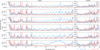 |
Fig. A.1 Planet-to-star (blue line) vs anti-planet-to-star (red line) coherent flux ratios in the L and M bands on the six VLTI-UT baselines. Coherent flux oscillations typical of a binary target are present at the expected planet position, and absent at its antipodal position. |
Appendix B Phase correction
The measured fringe phase, Φ, is composed of the object fringe phase, Φobj, and additional OPD terms produced in the successive mediums along the line of sight:
![Mathematical equation: $\[\Phi(\lambda)=\Phi_{\mathrm{obj}}(\lambda)+\frac{2 \pi}{\lambda}\left[\delta_{\mathrm{vac}}+\delta_{\mathrm{atm}}(\lambda)+\delta_{\mathrm{DL}}(\lambda)+\delta_{\mathrm{NCP}}\right],\]$](/articles/aa/full_html/2025/12/aa53323-24/aa53323-24-eq40.png) (B.1)
(B.1)
in which δvac, δatm, δDL, and δNCP are the OPDs between telescopes in vacuum, the atmosphere, the delay lines, and the non-common path between GRAVITY and MATISSE, respectively. A schematic view is offered in Fig. B.1. Due to the line of sight inclination relative to the telescope baseline, the light along one of the paths travels, in vacuum, an additional distance, Δd, resulting in the following achromatic vacuum OPD:
![Mathematical equation: $\[\delta_{\mathrm{vac}}=d_{\mathrm{vac}}-\left(d_{\mathrm{vac}}+\Delta d\right)=-\Delta d.\]$](/articles/aa/full_html/2025/12/aa53323-24/aa53323-24-eq41.png) (B.2)
(B.2)
This additional travel length is then compensated in air in the VLTI delay lines located in the common path, generating a chromatic common-path OPD:
![Mathematical equation: $\[\begin{aligned}\delta_{\mathrm{DL}} & =n_{\mathrm{DL}, ~1}(\lambda)\left(d_{\mathrm{DL}}+\Delta d\right)-n_{\mathrm{DL}, ~2}(\lambda) d_{\mathrm{DL}} \\& =\Delta n_{\mathrm{DL}}(\lambda) d_{\mathrm{DL}}+n_{\mathrm{DL}, ~1}(\lambda) \Delta d.\end{aligned}\]$](/articles/aa/full_html/2025/12/aa53323-24/aa53323-24-eq42.png) (B.3)
(B.3)
In these equations and the next, the nm,i and dm,i terms designate, respectively, the refractive index and the geometrical length along path i in medium m. Δnm is the difference of refractive indices between two paths in medium, m. In the approximation of a locally plane-parallel atmosphere, we can consider that light travels the same distance along each path in the atmosphere. The chromatic OPD introduced by the atmosphere is therefore:
![Mathematical equation: $\[\delta_{\mathrm{atm}}=\left[n_{\mathrm{atm}, ~1}(\lambda)-n_{\mathrm{atm}, ~2}(\lambda)\right] d_{\mathrm{atm}}=\Delta n_{\mathrm{atm}}(\lambda) d_{\mathrm{atm}}.\]$](/articles/aa/full_html/2025/12/aa53323-24/aa53323-24-eq43.png) (B.4)
(B.4)
The sum of these three OPDs forms the common-path OPD that is seen both by GRAVITY and MATISSE:
![Mathematical equation: $\[\begin{aligned}\delta_{\mathrm{CP}}(\lambda) & =\delta_{\mathrm{vac}}+\delta_{\mathrm{atm}}(\lambda)+\delta_{\mathrm{DL}}(\lambda) \\& =\left(n_{\mathrm{DL}, ~1}(\lambda)-1\right) \Delta d+\Delta n_{\mathrm{DL}}(\lambda) d_{\mathrm{DL}}+\Delta n_{\mathrm{atm}}(\lambda) d_{\mathrm{atm}}.\end{aligned}\]$](/articles/aa/full_html/2025/12/aa53323-24/aa53323-24-eq44.png) (B.5)
(B.5)
The fringe tracker, GRA4MAT, measures the average of δCP(λ) in K band: ⟨δCP(λ)⟩K. It then calculates and sends the according shift to the delay lines to correct the K-band OPD to zero: dFT = ⟨δCP(λ)⟩K/⟨nDL(λ)⟩K. The common-path OPD corrected by the fringe tracker is therefore
![Mathematical equation: $\[\begin{aligned}\delta_{\mathrm{CP}}^{\text {corr }}(\lambda) & =\delta_{\mathrm{CP}}(\lambda)-n_{\mathrm{DL}}(\lambda) d_{\mathrm{FT}} \\& =\delta_{\mathrm{CP}}(\lambda)-\frac{n_{\mathrm{DL}}(\lambda)}{\left\langle n_{\mathrm{DL}}(\lambda)\right\rangle_K}\left\langle\delta_{\mathrm{CP}}(\lambda)\right\rangle_K \\& =\sum_j\left(\delta_j(\lambda)-\frac{n_{\mathrm{DL}}(\lambda)}{\left\langle n_{\mathrm{DL}}(\lambda)\right\rangle_K}\left\langle\delta_j(\lambda)\right\rangle_K\right),\end{aligned}\]$](/articles/aa/full_html/2025/12/aa53323-24/aa53323-24-eq45.png) (B.6)
(B.6)
in which δj is each of the three terms constituting δCP in Eq. (B.5).
In order to evaluate the higher limits of these three terms, we simulated them using an air refractive index model and some pessimistic assumptions on the ambient conditions in the lines of sight. We use the air refractive index description of Voronin & Zheltikov (2017) that provides a compact generalization of the Sellmeier equation from the ultraviolet to the far-infrared. We assumed a pessimistic difference of 2° C in temperature and 5% in humidity between two delay lines; and 5° C and 40% between two telescopes’ lines of sight in the atmosphere. We also assumed a maximal length difference between delay lines. The whole set of parameters is listed in Table B.1. We simulated the three common-path OPD terms of Eq. (B.5), corrected by the fringe tracker as in Eq. (B.6). The results are shown in Fig. B.2. We find that (nDL (λ) − 1) Δd is in general more than 10× larger than the other terms in L and M, except at the beginning of the bands. This term is in addition the easiest and more accurate to model, as sensors are available in the delay line tunnel to get the average delay-line temperature and humidity. The other terms are difficult to model as there is no differential sensing between delay lines and between paths in the atmosphere. We thus neglect them in our corrected common-path OPD model:
![Mathematical equation: $\[\begin{aligned}\delta_{\mathrm{CP}}^{\mathrm{corr}}(\lambda) & \approx\left(n_{\mathrm{DL}}(\lambda)-1\right) \Delta d-\frac{n_{\mathrm{DL}}(\lambda)}{\left\langle n_{\mathrm{DL}}(\lambda)\right\rangle_K}\left\langle\left(n_{\mathrm{DL}}(\lambda)-1\right) \Delta d\right\rangle_K \\& \approx\left(\frac{n_{\mathrm{DL}}(\lambda)}{\left\langle n_{\mathrm{DL}}(\lambda)\right\rangle_K}-1\right) \Delta d.\end{aligned}\]$](/articles/aa/full_html/2025/12/aa53323-24/aa53323-24-eq46.png) (B.7)
(B.7)
Our model for the fringe phase is therefore finally
![Mathematical equation: $\[\Phi^{\mathrm{corr}}(\lambda) \approx \Phi_{\mathrm{obj}}(\lambda)+\frac{2 \pi}{\lambda}\left[\left(\frac{n_{\mathrm{DL}}(\lambda)}{\left\langle n_{\mathrm{DL}}(\lambda)\right\rangle_K}-1\right) \Delta d+\delta_{\mathrm{NCP}}\right].\]$](/articles/aa/full_html/2025/12/aa53323-24/aa53323-24-eq47.png) (B.8)
(B.8)
In our reduction, we only fitted δNCP. The ![Mathematical equation: $\[\delta_{\text {CP}}^{\text {corr}}(\lambda)\]$](/articles/aa/full_html/2025/12/aa53323-24/aa53323-24-eq48.png) was modelled thanks to the path lengths, temperature, pressure, and humidity measured in the delay line tunnel and reported in the FITS header of the MATISSE frames. Before fitting, we additionally remove from the data and model the mean L-band phase to get the differential phase, a standard step in interferometry as the absolute phase reference is lost during fringe tracking:
was modelled thanks to the path lengths, temperature, pressure, and humidity measured in the delay line tunnel and reported in the FITS header of the MATISSE frames. Before fitting, we additionally remove from the data and model the mean L-band phase to get the differential phase, a standard step in interferometry as the absolute phase reference is lost during fringe tracking:
![Mathematical equation: $\[\Phi^{\mathrm{diff}}(\lambda)=\Phi^{\mathrm{corr}}(\lambda)-\left\langle\Phi^{\mathrm{corr}}(\lambda)\right\rangle_L.\]$](/articles/aa/full_html/2025/12/aa53323-24/aa53323-24-eq49.png) (B.9)
(B.9)
The final estimate of the object differential phase is the difference between the differential phase data and the fitted OPD model:
![Mathematical equation: $\[\Phi_{\mathrm{obj}}^{\mathrm{diff}}(\lambda) \approx \arg \left[\mathrm{e}^{\mathrm{i} \Phi^{\mathrm{diff}}(\lambda)} \mathrm{e}^{-\mathrm{i} \frac{2 \pi}{\lambda}\left(\delta_{\mathrm{CP}}^{\text {corr }}(\lambda)+\delta_{\mathrm{NCP}}\right)}\right].\]$](/articles/aa/full_html/2025/12/aa53323-24/aa53323-24-eq50.png) (B.10)
(B.10)
We show in Fig. B.3 the non-common path OPDs fitted in each frame and each baseline. We can see systematic differences between BCD configurations, and a slow linear drift during the two hours, highlighted by the linear fits on one of the BCD configurations. The fitted OPD drifts range from 0.8 to 7.0 μm/h depending on the baseline.
Assumptions in the simulation of the common-path OPD terms introduced in the line of sight.
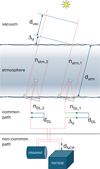 |
Fig. B.1 Schematics of a MATISSE + GRA4MAT observation, with the terms described in equations 1 to 5. |
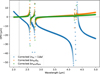 |
Fig. B.2 Simulation of the common-path OPD terms. The vertical dashed line shows the fringe tracking wavelength (2.2 μm), where the OPD is corrected to zero (horizontal dashed line). |
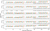 |
Fig. B.3 Temporal evolution of the non-common path OPD fitted on the data. The colours represent different BCD positions. The dashed line shows a linear fit on the frames using the IN-IN BCD position (blue crosses). The fit parameters and coefficient of determination are printed in each subplot. |
Appendix C Additional original datasets
Appendix C.1 GRAVITY
The new GRAVITY spectrum used in this paper has been built by taking the covariance-weighted mean of the contrast spectra of five β Pic b epochs from 2018 to 2022. The data was reduced with the exogravity pipeline (GRAVITY Collaboration 2020). The planet spectra of all epochs are shown in Fig. C.1, as well as the covariance-weighted average spectrum. We scaled the GRAVITY average contrast spectrum with the same stellar model as the one used for MATISSE.
Appendix C.2 NACO
β Pic b was observed on December 5, 2011 (programme 088.C-0196(A), PI S. Quanz) with VLT/NACO (Lenzen et al. 2003; Rousset et al. 2003), using the 172 mas slit, the L27_1_SL spectroscopic mode, the detector cube mode, and the HighDynamic / Double_RDRSTRD readout. These settings provide a wavelength coverage from 2.6 to 4.2 μm at a spectral resolution of ~350.
The slit was oriented so that both the central star and the planet (located at a separation of 450 mas and a position angle of 211.6° at the time of observation) were included. Nodding with an ABBA pattern was used to subtract background, but no extra jitter to ensure a maximum relative positioning stability. Star recentring was employed roughly every 40 minutes. A 180° camera rotation was also employed to reduce further instrumental artifacts such as ghosts. In all exposures the peak flux of the central star was kept below the linearity limit, roughly two thirds of the full dynamic range, including at the longest wavelengths (~4.1 μm) where the background emission dominates.
Each sequence of data was reduced separately using custom-made IDL scripts. A careful frame subtraction and spectrum extraction was then applied to the data cubes, as summarized hereafter. First, cubes for which the AO loop was opened and/or the Strehl ratio was low were rejected using statistical analysis. Then, sub-pixel shifts of the star position due to AO jitter were corrected using cross-correlation and sub-pixel shifts with a tanh interpolation kernel. Finally, positions of 17 telluric absorption features from ESO’s online DR05 Sky model (v1.2.0) were measured on the β Pic spectra and compared to the models to derive a wavelength calibration of the spectra. The result is a data cube containing the star and planet spectra along the slit in a 2D spatial-spectral map.
In order to subtract stellar contamination and extract the planet spectrum, we then applied a custom version of the so-called ‘spectral deconvolution’ algorithm (Sparks & Ford 2002; Vigan et al. 2008, 2012) to suppress most of the flux arising from the star. The algorithm uses the chromatic dependency of the stellar PSF and all its substructures (speckles and quasi-static aberrations) through the slit with respect to the fixed position of a companion to deblend the spectra of the two objects: each spectral channel i is rescaled by a factor λm/λi with λm the longest wavelength covered by the spectrum and λi the processed channel one. The rescaled slit is then composed of a series of nearly identical spectra of the star that can be median-combined to model the star spectrum while the companion spectrum is moving diagonally through the slit. This model spectrum is flux-normalized and subtracted from each stellar spectrum, leaving only the companion spectrum. As a final step, the spectral channels of the residual companion spectrum are scaled back to their original spatial resolution.
The level of residuals is strongly correlated to the position of the star within the slit, as the third Airy ring contaminates the planet spectrum at wavelengths longer than 3.5 μm for some stellar positions. We selected all non-contaminated spectra and extracted separately the planet spectrum in each. Spectra of β Pic b were divided by the stellar spectrum and multiplied by a blackbody function at the temperature of the star (8052 K, Gray et al. 2006) to remove telluric features. The averaged spectrum is shown in Figure 6. We masked zones with strong telluric residuals or where the extraction process left strong residuals.
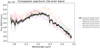 |
Fig. C.1 Compilation of GRAVITY spectra obtained at different epochs on β Pic b. The spectrum used in this paper is the weighted mean of all these spectra. |
Reported as the first direct emission spectrum of an exoplanet in the ESO-1002 press release. Spectra of a planetary-mass companion around a brown dwarf (2M1207 b, Chauvin et al. 2004), and a companion at the planet-brown dwarf mass boundary (AB Pic b, Chauvin et al. 2005), were, however, obtained earlier with NACO in the near-infrared.
Commissioning program 60.A-9257(H), see https://www.eso.org/sci/publications/announcements/sciann17548.html
For error calculation based on ellipses, see: https://simbad.u-strasbg.fr/Pages/guide/errell.htx
See the GRAVITY pipeline manual, v. 1.6.6.
All Tables
Relative astrometry of β Pic b found in our analysis, and predictions from the orbital fit of Lacour et al. (2021) retrieved with whereistheplanet.
Best-fit parameters using low (0.430 ± 0.001) and high (0.650 ± 0.001) Gaussian C/O priors, all other priors remaining unchanged.
Assumptions in the simulation of the common-path OPD terms introduced in the line of sight.
All Figures
|
Fig. 1 Simulation of the gain in contrast achieved by offsetting the pinhole of MATISSE on β Pic b, separated here by 534 mas from its host star. The upper and lower plots depict the stellar and planetary contribution to the coherent flux (the fringe envelope) as seen through the circular MATISSE pinhole (white area, hence the Airy-like shape of the output flux) centred on the star and on the planet, respectively. They are simulated at a wavelength of 3.5 μm and normalized to the maximal intensity of the star-centred stellar PSF. When the pinhole is centred on the planet, the speckle flux is reduced to the same level as the planetary flux. In each simulation, the asymmetric shape of the PSF of the offset object (relative to the pinhole) is due to imperfect spatial filtering of the Airy rings falling in the pinhole. |
| In the text | |
|
Fig. 2 Measured differential phase (grey dots) in two MATISSE frames, one on the star (top) and the other on the planet (bottom). Overlaid are the models presented in this work using the air refractive indices of Voronin & Zheltikov (2017) (blue), Mathar (2007) (green), and Ciddor (1996) (red). In the absence of chromatic or non-common path OPD, the differential phase should be zero on the star or an oscillation on the planet. |
| In the text | |
|
Fig. 3 Real (left) and imaginary (right) parts of the measured planet-to-star coherent flux ratio, ℱ, on the six UT baselines, during one 10 s frame. The error range is plotted in the background. The thick lines show the best-fit model as described in Sect. 4.1. It includes the star–planet modulation, the stellar speckle contamination (dashed blue curves), and the planet-to-star contrast assumption (dashed black curve). |
| In the text | |
|
Fig. 4 Scaling of the BT-Nextgen stellar model (Teff = 7890 K, log g = 3.83, [Fe/H] = 0.0) with species using Tycho, Gaia, and 2MASS photometry of β Pictoris. The bottom panel shows the residuals of the fit. |
| In the text | |
|
Fig. 5 Detection maps of β Pic b with MATISSE. The maps show the reduced χ2 values after fitting the stellar contamination for each tested planet astrometry (Δα, Δδ) in the grid. The grids are centred on MATISSE’s pointing during the planet observations. The left map is the size of the pinhole (1.5λ/D at 3.5 μm) and has a resolution of 1 mas. The right map was generated at higher resolution (0.1 mas) on a smaller 20 × 20 mas grid. The most likely astrometry from the MATISSE observations is shown as a blue ellipse, found by fitting a 2D Gaussian curve on the lowest |
| In the text | |
|
Fig. 6 Spectrum of β Pic b with MATISSE (black, this work) compared to other instruments: NACO (yellow, new data), GPI (blue, Chilcote et al. 2017), GRAVITY (green, new data) and MIRI (red, Worthen et al. 2024). Only the slope of the NACO spectrum can be compared to MATISSE as the absolute level was scaled manually. MATISSE data with a S/N < 5, located in strong telluric bands and not used in this work, are shown in grey. The absorption curves of H2O, CO, and CH4, calculated from the best-fitting Exo-REM model presented in Sect. 5, are plotted at the top to visualize their impact on the spectrum. H2O and CO leaves a visible pattern, but not CH4, likely because it is dominated by H2O absorption or buried in noise. |
| In the text | |
|
Fig. 7 Covariance (upper right triangle) and correlation (lower left triangle) matrices of the MATISSE spectrum of β Pic b. In order to highlight the off-diagonal correlations in the L band, the covariance values are clipped between 3 × 10⁻³⁵ and 3 × 10⁻³³ W2 m−4 μm−2 and the correlation values between 0.01 and 1. Two lines of off-diagonal correlations are further highlighted with arrows for readability. |
| In the text | |
|
Fig. 8 GRAVITY and MATISSE spectra of β Pic b with the best-fit Exo-REM models. The top plot shows the best fits on GRAVITY only, MATISSE only, and GRAVITY+MATISSE, when no scaling is applied on the spectra. The two other plots show the best fits on GRAVITY+MATISSE when a scale factor is applied either on MATISSE (middle) or on GRAVITY (bottom). |
| In the text | |
|
Fig. 9 Corner plot of the joint fit of GRAVITY (freely scaled) and MATISSE (fixed) spectra, using ForMoSA and the Exo-REM model grid. |
| In the text | |
|
Fig. 10 Fit of Exo-REM models using low (pink) and high (blue) C/O priors, compared to the free uniform C/O prior (green) already presented in Fig. 8. |
| In the text | |
|
Fig. 11 Signal-to-noise ratio calculated on the MATISSE contrast spectrum of β Pic b. |
| In the text | |
|
Fig. 12 Angular separations and L-band fluxes of a sample of exoplanets and brown dwarfs. Fluxes are either directly taken from the literature (blue points) or computed with ATMO and/or ExoREM models using atmospheric parameters fitted in the literature (red points). Minimal and maximal separations are represented as segments, while the current position of the planet is marked with an asterisk (except for β Pic c and HD 206893 c that are currently well below the MATISSE inner working angle). |
| In the text | |
|
Fig. A.1 Planet-to-star (blue line) vs anti-planet-to-star (red line) coherent flux ratios in the L and M bands on the six VLTI-UT baselines. Coherent flux oscillations typical of a binary target are present at the expected planet position, and absent at its antipodal position. |
| In the text | |
|
Fig. B.1 Schematics of a MATISSE + GRA4MAT observation, with the terms described in equations 1 to 5. |
| In the text | |
|
Fig. B.2 Simulation of the common-path OPD terms. The vertical dashed line shows the fringe tracking wavelength (2.2 μm), where the OPD is corrected to zero (horizontal dashed line). |
| In the text | |
|
Fig. B.3 Temporal evolution of the non-common path OPD fitted on the data. The colours represent different BCD positions. The dashed line shows a linear fit on the frames using the IN-IN BCD position (blue crosses). The fit parameters and coefficient of determination are printed in each subplot. |
| In the text | |
|
Fig. C.1 Compilation of GRAVITY spectra obtained at different epochs on β Pic b. The spectrum used in this paper is the weighted mean of all these spectra. |
| In the text | |
Current usage metrics show cumulative count of Article Views (full-text article views including HTML views, PDF and ePub downloads, according to the available data) and Abstracts Views on Vision4Press platform.
Data correspond to usage on the plateform after 2015. The current usage metrics is available 48-96 hours after online publication and is updated daily on week days.
Initial download of the metrics may take a while.