| Issue |
A&A
Volume 704, December 2025
|
|
|---|---|---|
| Article Number | A36 | |
| Number of page(s) | 14 | |
| Section | Interstellar and circumstellar matter | |
| DOI | https://doi.org/10.1051/0004-6361/202554308 | |
| Published online | 28 November 2025 | |
The factors that influence protostellar multiplicity
II. Gas temperature and mass in Perseus with APEX
1
Instituto de Astronomía, Universidad Nacional Autónoma de México, AP106, Ensenada CP 22830,
B.C.,
Mexico
2
Star and Planet Formation Laboratory, RIKEN Pioneering Research Institute,
Wako,
Saitama
351-0198,
Japan
3
Fox2Space – FTSCO, The Fault Tolerant Satellite Computer Organization,
Weigunystrasse 4,
4040
Linz,
Austria
4
Institute of Astronomy, Department of Physics, National Tsing Hua University,
Hsinchu,
Taiwan
5
Taiwan Astronomical Research Alliance (TARA),
Taiwan
6
Academia Sinica Institute of Astronomy and Astrophysics,
No. 1, Section 4, Roosevelt Road,
Taipei
10617,
Taiwan
7
NRC Herzberg Astronomy and Astrophysics,
5071 West Saanich Rd,
Victoria,
BC V9E 2E7,
Canada
8
Department of Physics and Astronomy, University of Victoria,
Victoria,
BC V8P 5C2,
Canada
9
Department of Physics, Norwegian University of Science and Technology,
7491
Trondheim,
Norway
10
Independent researcher,
Sagas Väg 5,
43431
Kungsbacka,
Sweden
★ Corresponding author: This email address is being protected from spambots. You need JavaScript enabled to view it.
Received:
27
February
2025
Accepted:
15
October
2025
Abstract
Context. Protostellar multiplicity is a common outcome of the star formation process. To fully understand the formation and evolution of these systems, the physical parameters of the molecular gas together with the dust must be systematically characterized.
Aims. Using observations of molecular gas tracers, we characterize the physical properties of cloud cores in the Perseus molecular cloud (average distance of 295 pc) at envelope scales (5000-8000 AU).
Methods. We used Atacama Pathfinder EXperiment (APEX) and Nobeyama 45m Radio Observatory (NRO) observations of DCO+, H2CO, and c-C3H2 in several transitions to derive the physical parameters of the gas toward 31 protostellar systems in Perseus. The angular resolutions ranged from 18" to 28.7", equivalent to 5000-8000 AU scales at the distance of each subregion in Perseus. The gas kinetic temperature was obtained from DCO+, H2CO, and c-C3H2 line ratios. Column densities and gas masses were then calculated for each species and transition. Gas kinetic temperature and gas masses were compared with bolometric luminosity, envelope dust mass, and multiplicity to search for statistically significant correlations.
Results. Gas kinetic temperature derived from H2CO, DCO+, and c-C3H2 line ratios have average values of 26 K, 14, and 16 K, respectively, with a range of 10-26 K for DCO+ and c-C3H2. The gas kinetic temperature obtained from H2CO line ratios have a range of 13-82 K. Column densities of all three molecular species are on the order of 1011 to 1014 cm−2, resulting in gas masses of 10−11 to 10−9 M⊙. Statistical analysis of the physical parameters finds: i) similar envelope gas and dust masses for single and binary protostellar systems; ii) multiple protostellar systems (>2 components) tend to have slightly higher gas and dust masses than binaries and single protostars; iii) a continuous distribution of gas and dust masses is observed regardless of separation between components in protostellar systems.
Key words: astrochemistry / methods: observational / methods: statistical / stars: formation / stars: low-mass / ISM: molecules
© The Authors 2025
 Open Access article, published by EDP Sciences, under the terms of the Creative Commons Attribution License (https://creativecommons.org/licenses/by/4.0), which permits unrestricted use, distribution, and reproduction in any medium, provided the original work is properly cited.
This article is published in open access under the Subscribe to Open model. This email address is being protected from spambots. You need JavaScript enabled to view it. to support open access publication.
1 Introduction
Most stars are found to be in multiple stellar systems, with companion frequencies increasing with mass (see Offner et al. 2023 and references therein). This demonstrates that multiplicity is a central aspect and general outcome of the star formation process across time. Observations of starless cores in various star-forming regions have sought to identify substructures linked to fragmentation (Perseus: Schnee et al. 2010; Taurus: Hacar & Tafalla 2011; Caselli et al. 2019; Ophiuchus: Kirk et al. 2017; Chamaeleon I: Dunham et al. 2016). These studies have mixed results, with the lack of substructure attributed to the evolutionary stage, mechanism of collapse, or observational limitations. Dust continuum studies have provided information on protostellar multiplicity and companion fractions, and the distribution of components within cloud cores, and speculated on formation
mechanisms (e.g., Looney et al. 2000; Chen et al. 2013; Mairs et al. 2016; Tobin et al. 2016; Sadavoy & Stahler 2017; Encalada et al. 2021; Tobin et al. 2022; Offner et al. 2023). While these studies provide a rough temperature and mass estimate from the dust, they lack detailed information on the physical conditions of the gas. Various key parameters of star formation that are essential ingredients for simulations and that link observations to theoretical studies can only be provided by atomic and molecular gas observations (e.g., Mairs et al. 2014; Luo et al. 2022; Chen et al. 2024; Neralwar et al. 2024).
The Perseus molecular cloud has been extensively studied. A few examples of studies from the last decade have explored cloud structure (e.g., Hacar et al. 2017; Chen et al. 2020), line emission (e.g., Higuchi et al. 2018; Hsieh et al. 2019; Yang et al. 2021; Tafalla et al. 2021; Dame & Lada 2023), multiplicity (e.g., Pineda et al. 2015; Tobin et al. 2016; Murillo et al. 2016; Sadavoy & Stahler 2017; Pokhrel et al. 2018), and polarization (e.g., Doi et al. 2021; Coudé et al. 2019; Choi et al. 2024).
Given this wealth of information, Perseus is an excellent region in which to study the factors that affect multiplicity in star formation. Furthermore, the Perseus molecular cloud presents a range of star-forming environments. Externally irradiated subregions such as IC348 and NGC1333 contrast with isolated environments such as L1455, B1, and L1448. Clustered subregions, such as NGC1333, and non-clustered environments, such as L1448, are also found in the Perseus molecular cloud (Plunkett et al. 2013). The distance to these subregions varies between 279 and 302 pc, with an average distance of 294 pc (Zucker et al. 2018). More recent work using the LAMOST DR8, 2MASS PSC, and Gaia EDR3 data (Cao et al. 2023) find consistent distances for Perseus.
A pilot study of ten protostellar systems in Perseus with the Atacama Pathfinder EXperiment (APEX, Güsten et al. 2006) was carried out with the aim of studying the temperaturemultiplicity relation at envelope scales (~8000 AU, Murillo et al. 2018a, hereafter pilot paper). The observations targeted DCO+, H2CO, c-C3H2, and 13CO in the 230 and 360 GHz APEX bands. This study suggested a lack of correlation between temperature and multiplicity, but instead suggested a mass-multiplicity relation. However, statistically significant conclusions could not be obtained due to the sample size of ten protostellar systems.
Expanding the sample size to 37 protostellar systems observed with on-the-fly (OTF) maps using the Nobeyama 45m Radio Observatory (NRO) and targeting HNC, HCN, N2H+, and HCO+ enabled a more statistically significant study of the temperature and mass relations with respect to protostellar multiplicity at scales of 5000 AU (Murillo et al. 2024, hereafter Paper I). The gas kinetic temperature was derived using the I(HcN)/I(HNC) J =1-0 ratio (Graninger et al. 2014; Hacar et al. 2020), and compared to NH3 temperatures (Friesen et al. 2017) and dust temperatures (Zari et al. 2016). The study was further complemented with APEX HNC J=4-3 single-pointing observations in order to derive H2 volume density from the HNC J=4-3/J =1-0 ratio. No relation between multiplicity and gas kinetic or dust temperature was found in Paper I, as was suggested in the pilot paper. A relation between mass and the degree of multiplicity was found in Paper I, with a continuous mass distribution independent of component separation. This finding suggests a continuum in formation mechanisms for multiple protostellar systems, rather than distinct core and disk mechanisms for close and wide separations in multiple protostellar systems. This result is consistent with the existence of equal mass wide binaries (e.g., El-Badry et al. 2019), outspiraling due to gas accretion causing binaries to widen (e.g., Mignon-Risse et al. 2023), and dynamical capture with efficient inspiraling (e.g., Kuruwita & Haugbølle 2023).
The aim of the present study is to explore the relation between multiplicity, mass, and temperature using molecular species that trace the inner regions and structures of protostellar cores. Different molecular species probe different structures and temperature regimes within protostellar cores (e.g., Tychoniec et al. 2021). In protostellar cloud cores where CO is abundant, formylium (DCO+) is enhanced when CO begins to freeze out onto dust grains. In protostellar envelopes, DCO+ is found between the CO freeze-out temperature (20 to 30 K, Jørgensen et al. 2005) and the desorption density of CO (~104 cm−3). It is useful to note that DCO+ also has a warm formation path at gas temperatures above 30 K, mostly present around the disk for embedded protostars (Favre et al. 2015). Previous observations showed that warm DCO+ is more readily detected in the J=5-4 transition with interferometric data, but is less prominent in single-dish observations (Murillo et al. 2018b). This means that the DCO+ emission in the present study traces the cool regions of the protostellar envelope (e.g., Mathews et al. 2013; Murillo et al. 2015). Formaldehyde (H2CO) is an excellent thermal probe of gas between 30 and 100 K, with the gas kinetic temperature increasing proportional to the line ratio. Irradiated environments (e.g., outflow cavities) are best traced with species such as cyclo-propenylidene (c-C3H2; e.g., Drozdovskaya et al. 2015; Murillo et al. 2018a; Tychoniec et al. 2021). Each set of molecular line emission ratios provides an independent measurement of the gas kinetic temperature averaged over the beam area of the observations. DCO+ J=5-4/J =3-2 provides the gas kinetic temperature of the cold inner envelope. The H2CO and c-C3H2 ratios can provide gas kinetic temperatures of the warm inner envelope and irradiated outflow cavity walls, respectively. The derived temperatures are compared to source parameters (bolometric luminosity, dust mass, and multiplicity) to search for correlations. Because each species traces a different structure within the cloud core, they can be used to probe the amount and distribution of material available for accretion around protostellar sources (envelope versus outflow cavity). The per-species beam-averaged column density and gas mass derived from DCO+, H2CO, and c-C3H2 thus enables the comparison of masses, per species, versus multiplicity in the inner regions of protostellar cores.
This work presents single-dish observations toward five subregions in the Perseus molecular cloud. The observations target 31 protostellar systems using APEX single-pointing observations of DCO+, H2CO and c-C3H2, complemented with NRO OTF maps of DCO+ J =1-0. Observational data details are provided in Sect. 2. Section 3 describes the results of the observations. The derivation of physical parameters and the statistical analysis are explained in detail in Sect. 4. Finally, the discussion and conclusions of this work are provided in Sects. 5 and 6.
2 Observations
2.1 Sample
The source sample included in this work is composed of 31 protostellar systems, selected based on the region overlap between APEX and the NRO OTF maps of DCO+ J=1-0. The sample contains the ten protostellar systems from the pilot paper (hereafter, pilot sample) to complement newer APEX observations (hereafter, extended sample). The mini cluster NGC1333 IRAS4, observed in the NRO OTF map but not in the APEX single pointings, is included in the sample. The sample in this work contains 19 multiple protostellar systems and 12 single protostellar sources distributed in five subregions of Perseus: NGC1333, L1448, L1455, B1, and IC348. Among the 19 multiple protostellar systems, eight systems are close binaries, five systems are wide binaries, and six systems are higher-order multiples (three or more components within a common cloud core). Close and wide binaries are defined following the criteria used in Murillo et al. (2016); namely, that close binaries are those that have separations <7" (2100 AU at d = 300 pc) and that are not resolved in Herschel PACS (Poglitsch et al. 2010) observations. A pointing with APEX was made for each component of a protostellar system that can be resolved in Herschel PACS images. This implies that higher-order multiples and wide binary systems have several pointings per system, while close binaries and single protostars have one pointing per system. Higher-order multiples can have unresolved components; for example, NGC1333 SVS13A and L1448 N-B have components with separations <7,,. Hence, the 31 systems included in the sample were observed with 46 pointings. Table A.1 lists the systems and pointings used in this work.
2.2 Dust continuum parameters: Lbol and Menv
Two parameters obtained from dust continuum observations are used in this work: bolometric luminosity, Lbol, and envelope dust mass, Menv. The Lbol parameter was obtained from the spectral energy distribution (SED) of the source using trapezoidal integration with the equation
 (1)
(1)
where d is the distance and Sν is the flux at a given frequency, ν. The SEDs were taken from Murillo et al. (2016) and include Spitzer, Herschel PACS, and (sub)millimeter fluxes. For any two components that have separations of ≥7″, their Lbol values are for the individual protostars. In contrast, components with separations of <7″ have Lbol values that are the arithmetic average of the luminosity of both protostellar components. The 7″ limit is due to the spatial resolution of Herschel PACS data used in the SEDs. A detailed exploration of bolometric luminosity toward unresolved protostellar component pairs is given in Murillo et al. (2016).
For the envelope dust mass, we used the method from Jørgensen et al. (2004), which is given by
 (2)
(2)
where Menv was calculated from the 850 μm dust continuum peak intensity, S850 μm. The James Clerk Maxwell Telescope (JCMT) Gould Belt Survey SCUBA-2 data release 3 (GBS DR31; Kirk et al. 2018; Chen et al. 2016; Pattle et al. 2025) 850 μm maps were used to obtain the peak fluxes for the sources in our sample. Since previous papers (pilot paper and Paper I) used peak fluxes from the COMPLETE survey (Ridge et al. 2006), a comparison of the envelope dust masses derived from SCUBA-2 and SCUBA peak fluxes is presented in Appendix B.
For both parameters, Lbol and Menv, the adopted distances per subregion are 288 pc for L1448, 299 pc for both NGC1333 and L1455, 301 pc for B1, and 295 pc for IC348 (Zucker et al. 2018). Both Lbol and Menv are listed in Table A.1 and included in the CDS online data for the current work.
2.3 Atacama Pathfinder Experiment (APEX)
The pilot sample of ten protostellar systems was observed with the Swedish Heterodyne Facility Instrument (SHeFI; Nyström et al. 2009; Vassilev et al. 2008) receivers APEX-1 (O-098.F-9320B.2016, NL GTO time) and APEX-2 (M-099.F-9516C-2017) on 1 December 2016 and 7-12 July 2017, respectively. The extended sample was observed using the PI230 and First Light APEX Submillimeter Heterodyne (FLASH+; Klein et al. 2014) receivers in single pointing mode. Observations with PI230 (O-0104.F-9307A) were carried out on three dates: 8 July, 11 July, and 12 October 2019. FLASH+ observations (O-0104.F-9307B) were done on six dates: 11, 15-18, and 20 October 2019. The extended sample targeted 27 protostellar systems, but only 21 are included in this work due to them overlapping with the NRO OTF maps of DCO+.
The receivers APEX-1 and APEX-2 were used to observe the pilot sample in two spectral settings with central frequencies 217.11258 and 361.16978 GHz, and a bandwidth of 4 GHz. Full details are given in the pilot paper and briefly described here. The APEX-1 spectral setup targeted DCO+ J =3-2, three transitions of H2CO, and three transitions of c-C3H2. APEX-2 was used to observe DCO+ J=5-4 and H2CO J=5-4. Typical noise levels range between 15 to 70 mK for APEX-1, and 20 to 100 mK for APEX-2, for a channel width of 0.4 km s−1, and HPBW of 28.7″ and 18″, respectively. The adopted beam efficiencies were ηmb = 0.75 and 0.73, for APEX-1 and APEX-2, respectively.
The central frequency of PI230 was set to 217.11258 GHz, mainly targeting DCO+ J=3-2, three transitions of H2CO, and three transitions of c-C3H2. The 7.5 GHz bandwidth of PI230 also included additional molecular species (DCN J=3-2, C18O J=2-1, 13CO J=2-1, two transitions of SO, and one transition of CH3OH) that will be treated in future work. Typical noise levels for the observations ranged between 10 to 30 mK for a channel width of 0.4 km s−1 and a HPBW of 28.7″. The beam efficiency, ηmb, for PI230 observations at 230 GHz is 0.8.
The spectral setup with FLASH+ targeted DCO+ J=5-4, H2CO J=5-4, DCN J=5-4, and HNC J=4-3, with a central frequency of 361.16978 GHz and a bandwidth of 4 GHz. The HNC J=4-3 data has been reported in Paper I, and DCN J=5-4 will be discussed in a future work. Typical noise levels for the observations ranged between 18 and 145 mK for a channel width of 0.4 km s−1, and a HPBW of 18″. A beam efficiency of ηmb = 0.73 was adopted, based on the APEX-2 beam efficiency at 352 GHz.
The GILDAS/CLASS software package2 (Gildas Team 2013) was used to perform standard calibration. All spectra were averaged to 0.4 km s−1 in order to increase the sensitivity. Sample spectra for three systems are briefly discussed in Appendix C and shown in Fig. C.1. The averaged spectra results in detection in at least two channels for the weakest lines, and three or more channels for stronger line emission. Spectral line parameters (peak, width, root-mean-square, RMS, noise levels) for all APEX data were measured with the GILDAS/CLASS Gaussian fitting routines. Targeted molecular species and their respective parameters are listed in Table 1.
The system Per25, an isolated single protostellar source in L1455, was included in both the pilot and extended samples (Fig. C.2). Hence it is used to compare the quality of both datasets. The extended sample has lower noise (20-60 mK with Δv = 0.4 km s−1) relative to the pilot sample (25-100 mK with Δv = 0.4 km s−1). In the extended sample observations, six molecular lines are detected toward L1455 Per25 with > 3σ DCO+ J=3-2, HNC J=4-3, H2CO J=30,3-20,2, and the three transitions of c-C3H2. In the pilot observations, only two detections were above 3σ for L1455 Per25, DCO+ J=3-2 and HNC J=4-3, while the others were undetected or marginal (< 3σ). Thus, the extended sample observations provide a better constraint for single protostars than the pilot sample observations.
2.4 Nobeyama 45 m Radio Observatory (NRO)
The DCO+ J=1-0 observations of Perseus with the NRO were made using the FOur-beam REceiver System on the 45m Telescope (FOREST; Minamidani et al. 2016) frontend and the Spectral Analysis Machine for the 45 m Telescope (SAM45;Kamazaki et al. 2012) backend. Observations (G22019 PI: N.M. Murillo) were carried out between February and April 2023. The objective of these observations was to make OTF maps similar to those presented in Paper I but targeting the corresponding deuterated species. In the current work, only the DCO+ J =1-0 spectral data averaged over 23″ beams were used. The remaining data will be presented in a future work.
For the DCO+ OTF map, the channel resolution is 30.52 kHz (-0.1 km s−1) with a bandwidth of 125 MHz. The OTF map pixel size is 6″. Noise levels ranged between 0.1 and 0.5 K, with an angular resolution of 23″. We adopted a beam efficiency of ηmb of 0.6 based on the data provided in the NRO website. The value was interpolated from the measurements by NRO for the 20222023 observing season3, since the frequency of DCO+ J=1-0 (72 GHz) is not standard operation for FOREST.
Standard data calibration and imaging for each datacube were done with the NOSTAR software package provided by NRO. Gaussian fitting to extract the spectral line peak, width, and noise level from the map were performed using the bettermoments Python library (Teague & Foreman-Mackey 2018; Teague 2019).
Molecular species in this work.
3 Results
In this work, we focus on three transitions of DCO+ and c-C3H2, and four transitions of H2CO. Transitions, frequencies, and beam sizes for each molecular species are listed in Table 1 along with the range of line peaks, RMS noise levels, and line widths for each species and transition. All the measured and derived values from the data used in this work will be made available online at CDS.
To ensure that the results presented in this work are not biased due to sample selection, the rate of detections per molecular transition was counted. Detection fractions were examined relative to the full sample, system multiplicity, region clustering, and system parameters (bolometric luminosity, Lbol, and envelope dust mass, Menv).
In general, detection rates are inversely proportional to frequency regardless of the sample binning used. For the sample in our work, p-H2CO J=30,3-20,2 is detected in 92% of systems, while J=32,2-22,1 and J=32,1-22,0 are only detected in fewer than 40% of systems. Two transitions of c-C3H2, J=33,0-22,1 and J=6-5, are detected with a rate above 70%, while the J=51,4-42,3 transition is detected in 59% of systems. Similarly, DCO+ J=3-2 is detected in 92% of the full sample, while the J=5-4 transition is detected in 60% of systems. The DCO+ J =1-0 transition is detected in all sources located within the OTF maps.
When considering detection rates versus multiplicity, sources show similar detection rates for the low transitions, while close binaries and single systems show similar detection frequencies for the higher transitions, which are typically about 20% lower than the multiple systems. Region clustering and Lbol does not affect detection frequencies. On the other hand, detection frequencies decrease proportionately with Menv. This is expected as lower mass leads to lower fluxes. Sources with Menv ≥ 1 M⊙ have 100% detection frequencies in most transitions (except H2CO J=32,2-22,1 and J=32,1-22,0, with ~60 and ~80 % detection frequencies, respectively). For sources with Menv < 0.1 M⊙, the detection frequency drops to 33% in the lowest transition of APEX observations, and no detection for higher transitions.
4 Analysis
4.1 Gas kinetic temperature
The availability of two or more transitions per molecular species in the APEX data enables estimates of the gas kinetic temperature through the use of line peak ratios. The 218 and 360 GHz data have spatial resolutions of 28.7″ and 18″, respectively (see Sect. 2.3). To calculate line ratios within a common area of 28.7″, a beam dilution factor of 0.39 was applied to the DCO+ J=5-4 and H2CO J=50,5-40,4 transitions. Applying the above beam dilution factor assumes that each line emission arises from a region that has the size of the corresponding beam, which might not be true for some sources or transitions. However, to determine the relative extent of each species and transition, higher-spatial-resolution data is needed. We then calculated line peak ratios using the peak brightness temperature from the APEX observations for the following transition pairs: DCO+ J=5-4/J =3-2; H2CO J=32,2-22,1/J=30,3-20,2, J=32,1-22,0/J=30,3-20,2, and J=50,5-40,4/J=30,3-20,2; and c-C3H2 J=6-5/J=33,0-22,1 and J=51,4-42,3/J=33,0-22,1. Only ratios for which the lower transition is detected with ≥3σ were considered. If the higher transition was not detected, the RMS noise level was adopted for that transition and the ratio was considered an upper limit. Propagation of uncertainty analysis was used to calculate the line peak ratio error, using the noise level of the respective spectra as the standard deviation and assuming a covariance of zero (uncorrelated variables).
Non-local thermal equilibrium (non-LTE) excitation and radiative transfer calculations using the off-line version of the program RADEX (van der Tak et al. 2007) with uniform sphere geometry together with molecular collisional data from the Leiden Atomic and Molecular Database (LAMDA, Schöier et al. 2005; van der Tak et al. 2020) were used to model the line peak ratios of DCO+, H2CO, and c-C3H2. We assumed that the emission from the different transitions of the same molecular species arise from the same region, and hence assumed that the material traced by the molecular species has a single density and temperature. Given that the Perseus molecular cloud dominates the emission along the line of sight (e.g., Doi et al. 2021), we assumed that there is no significant temperature gradient along the line of sight. The collisional rate coefficients for DCO+ are based on Botschwina et al. (1993) and Flower (1999), while for H2CO and c-C3H2 the collisional rate coefficients are based on Wiesenfeld & Faure (2013) and Chandra & Kegel (2000), respectively. The line peak ratio models consider a temperature range of 10 to 200 K, and a H2 volume density range of 103-1010 cm−3. Column densities of 1012 cm−2 and line widths of 1 km s−1 were adopted in the models. The chosen line width is based on the average line width of all detected species, with broader line widths likely to have contributions from outflow emission (Fig. C.1).
Gas kinetic temperatures, Tkin, were inferred by comparing the observed line peak ratios and known H2 volume densities with the RADEX models. The H2 volumetric densities from Paper I were derived from the HNC J=4-3/J=1-0 ratio and are mean values within ~5000 AU diameter regions, ranging from 105 to 106 cm−3. Increasing the adopted H2 volumetric density by an order of magnitude decreases the estimated Tkin by 5 K, at most, for all three molecular species used in this work. On the other hand, increasing or decreasing by an order of magnitude the adopted column density of a species in the RADEX models produces an average change of 2 K at most. The Tkin adopted in this work were estimated from the APEX line peak ratios and the Paper I H2 volume density values, and their respective uncertainties, without corrections for the 28″ beamsize (~8000 AU) of the APEX observations. This comparison resulted in a list of values for which the average and standard deviation were calculated in order to adopt a single Tkin value and uncertainty for each line peak ratio.
The Tkin values obtained from the three line peak ratios of H2CO vary by about 10 to 20 K. This variation is likely caused by the variety of structures contributing to the emission within the APEX beam. However, analyzing the individual Tkin values separately without spatially resolved maps of the emission would not provide deeper insights into the physical condition of each core. Hence, to avoid analyzing three separate Tkin values obtained from the three H2CO line peak ratios, the values were averaged together and this likely contributes to the spread in the H2CO Tkin values reported in this work. In the case of c-C3H2, the resulting Tkin values from the two line peak ratios differ by 5 K or less, suggesting a common emission source for the three transitions. Hence, the two separate Tkin values were averaged together.
The inferred Tkin are plotted against Lbol and Menv in Fig. 1. Gas kinetic temperatures derived from DCO+ and c-C3H2 show similar values of between 10 and 26 K. These values are consistent with Tkin,nH3 estimates toward Perseus from Rosolowsky et al. (2008), who found an average temperature of 11 K with a spread of 9 to 26 K from NH3 single pointing observations with the Green Bank Telescope (beam 31″), and Tkin from I(HCN)/1(HNC) J=1-0 maps (Paper I), which has an average value of 15 K. By-eye coordinate matching was used to find a common sample between the Rosolowsky et al. (2008) catalog and our sample. The Tkin,nH3 values for the common sample are plotted in Fig. 1 for comparison with the Tkin values derived in this work. On the other hand, H2CO ranges between 10 and 40 K, with one source showing a gas kinetic temperature of 80 K (NGC1333 IRAS5 Per63, outside the plotted range of Fig. 1) and another an upper limit of 54 K (L1455 Per25).
4.2 Column density
Using the observed peak brightness temperature and line width together with the H2 volumetric density (n(H2)) from Paper I, and the gas kinetic temperature (Tkin) derived in this work (Sect. 4.1), we derived the column density of each molecular species and transition from non-LTE calculations. The column density uncertainties were calculated by using the lower and upper limits of n(H2) and Tkin in the non-LTE RADEX calculations, and then taking the average and standard deviation of all three values. Column densities for the different transitions of the same molecular species are found to be similar, varying by up to 50%, with only a few cases varying by a factor of 2. The column density for each transition was calculated in several ways - using two values of Tkin (derived from I(HCN)/1(HNC) J=1-0 or corresponding line ratio) and varying n(H2) by an order of magnitude - the objective being to determine how much the choice of Tkin and n(H2) affects the calculated column density. For all molecular species, upper limits lead to severely under- or overestimated column densities.
The column density of DCO+ is not sensitive to the adopted gas kinetic temperature. Increasing n(H2) by an order of magnitude causes N(DCO+) to increase by a factor of 2 on average for J =3-2 and a factor of 4 on average for J=5-4. In the case of H2CO, increasing Tkin and n(H2) typically generates lower N(H2CO) column densities by a few percent. For c-C3 H2, changing Tkin does not cause significant changes in N(c-C3H2). Overall, the calculated column densities do not vary by one or more orders of magnitude unless one of the parameters is an upper limit.
The calculated column densities used in this work adopt the n(H2) from Paper I, and the Tkin from the corresponding molecular species (see Sect. 4.1). For DCO+ J =1-0, the Tkin from Paper I was adopted instead of the gas kinetic temperature derived from the J=5-4/J=3-2 ratio. All derived column densities are available in the CDS published data. The column densities for the lowest transition of DCO+, H2CO and c-C3H2 are plotted against Lbol and Menv in Fig. 1.
4.3 Gas mass
Different molecular species trace distinct temperature regimes and various physical structures. DCO+ traces the cold inner envelope where gaseous CO starts to freeze out. H2CO traces the inner warm envelope and outflow cavity. c-C3H2 traces the irradiated outflow cavity. In addition, not all sources present emission in all three species and their respective transitions (see Sect. 3). By calculating the gas mass of the three species, we can probe the amount and distribution of material available for the forming protostar and compare this distribution with multiplicity.
The gas mass for a molecular species X, Mgas,x, was derived in the same way as in Paper I, using the expression
 (3)
(3)
where Mr is the mean molecular weight (30.0237, 30.031, and 38.01565 g mol−1 for DCO+, H2CO, and c-C3H2, respectively), NA is Avogadro’s constant, N(X) is the derived gas column density for X molecule, A is the beam area over which the mass is calculated, and Msun,g is the solar mass in grams. Adopted distances per subregion are 288 pc for L1448, 299 pc for NGC1333 and L1455, 301 pc for B1, and 295 pc for IC348 (Zucker et al. 2018). The beam diameters are listed in Table 1. The uncertainty was obtained with the same equation, but with N(X) being the uncertainty of the derived column density and all other parameters assumed to be constant. The derived Mgas,x are plotted against Menv in Fig. 2. All derived gas masses are available in the CDS published data. Derived gas masses are consistent between transitions, showing similar values and trends, in particular the trend of gas mass increasing proportionately to Menv. The gas mass obtained from H2CO shows a larger spread than the gas masses from DCO+ and c-C3H2.
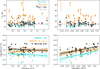 |
Fig. 1 Physical parameters derived from APEX observations. Top row : gas kinetic temperature and corresponding errors obtained from molecular line ratios. Cyan circles show the temperature obtained from DCO+ J=5-4/J=3-2, orange squares show the average temperature obtained from the three H2CO ratios, and black diamonds show the average temperature obtained from the two c-C3H2 ratios. Upper limits are indicated with a downward arrow. The horizontal dash-dotted red line indicates the average gas kinetic temperature (Tkin ~15 K) derived from the I(HCN)∕I(HNC) J =1-0 (Paper I). The gray crosses show the gas kinetic temperature from NH3 observations (Tkin,NH3) obtained from the core catalog of Rosolowsky et al. (2008). The left and right panels plot gas kinetic temperature versus bolometric luminosity (Lbol) and envelope dust mass (Menv), respectively. Bottom row : column density for DCO+ (cyan circles), H2CO (orange squares), and c-C3H2 (black diamonds) obtained from the respective lowest transition in the APEX data. Solid lines and shaded areas show the linear regression for the data with the corresponding color. The left and right panels plot column density versus Lbol and Menv. Error bars are smaller than the symbols. |
4.4 Statistical analysis
To examine the relations between the physical parameters derived in this work and the multiplicity of the sample, a statistical correlation test was performed. The generalized Kendall’s rank correlation (Isobe et al. 1986) was applied to our data using standard Python libraries and following the method used in the pilot paper. This method enables the degree of association between two quantities with censored (upper limit) data to be measured. For this work, Lbol and Menv were tested against gas kinetic temperature and gas mass. The null hypothesis of the generalized Kendall’s rank correlation is that the values are uncorrelated. Hence, p values <0.05 indicate a correlation at a higher than 3σ significance.
Four classification schemes, listed in Table 2, are used for statistical analysis. These classification schemes follow those used in Paper I, except for multiplicity within the beam (Scheme 2 in Paper I), which was not followed due to the different angular resolutions of the APEX and NRO data (Table 1). Bin sizes in each classification scheme vary according to the molecular species used to derive the physical parameter being tested. This occurs because not all sources have detections in all transitions of each molecular species. A system in this work is considered to be all the protostars within a common core, assuming gravitational boundness for simplicity. This definition leads to the gas and dust mass of a system being equal to the sum of the masses of each of its components, while the gas kinetic temperature and column densities are averaged over all components.
Gas kinetic temperatures do not show a correlation to Lbol regardless of the classification scheme. The generalized Kendall’s rank correlation only finds p values <0.05 between Menv and Tkin from DCO+ J=5-4/J =3-2 for the full sample. In the other three classification schemes, the correlation only appears in the single protostar bin. The reason for this result is unclear, and may require data that spatially resolve the molecular line emission to explain. As is expected from Fig. 1, the slope of the Tkin versus Lbol or Menv is flat.
Gas mass, Mgas,x, from the three molecular species is uncorrelated to Lbol in any of the classification schemes. In contrast, Mgas,x from the three molecular species studied shows a correlation to Menv in the four classification schemes.
In Fig. 3, the general trend from Mgas,N2H+ 4 reported in Paper I is shown for reference and comparison. All of the gas masses derived in this work are about two orders of magnitude lower than the Mgas,N2H+ but with a similar slope. Mgas,DCO+, Mgas,H2CO, and Mgas,c-C3H2, are similar to Mgas,HCO+. This is likely produced by the molecular species and transitions used in this work tracing the inner regions of the protostellar cores, which naturally have less material within the beam than N2H+. It is unlikely to stem from chemical processes (e.g., fractionation) due to the lack of correlation between Mgas,x and Tkin or Lbol.
In classification schemes 2 and 4, Mgas,DCO+ and Menv exhibit a correlation for all multiplicity bins, with multiple systems showing slightly higher masses than binary and single protostars (Fig. 3, left column). In classification scheme 3, the multiple systems do not show a significant correlation between Menv and Mgas,DCO+ or Mgas,c-C3H2, which may be due to the bin sample size of five and four systems. For H2CO (Fig. 3, center column), classification schemes 2 and 3 do not show significant correlations between multiple systems and mass (bin sample sizes of 10 and 5, respectively). Binaries in classification scheme 2 (bin sample size of 7) also do not show a significant correlation between Mgas,H2CO and Menv. The spread in values derived from H2CO may also contribute to weakening any correlation if it exists. Finally, Mgas,c-C3H2 (Fig. 3, right column) has a smaller spread than Mgas,H2CO. Single systems in classification schemes 2 to 4 do not show correlations between Mgas,c-C3H2 and Menv, while binary systems do not show a correlation between Mgas,c-C3H2 and Menv in classification scheme 2. Multiple systems show correlations in classification schemes 2 and 4 (bin sample sizes of 9 and 14, respectively) and generally higher Mgas,c-C3H2 and Menv than singles and binaries.
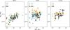 |
Fig. 2 Gas mass (Mgas) versus dust mass (Menv) for all transitions of DCO+ (left panel), H2CO (center panel), and c-C3H2 (right panel). This plot shows that the gas masses from DCO+ and c-C3H2 are consistent between transitions, while H2CO shows a broader spread. In the center panel, the gas mass from H2CO 32,2-22,1 is not shown to avoid a crowded plot, but follows a similar distribution to the other transitions shown in the panel. |
Classification schemes for statistical analysis.
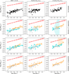 |
Fig. 3 Relations of the DCO+ J =1-0 gas mass (MDCO+, left column), H2CO J=30,3-20,2 gas mass (MH2CO, center column), and c-C3H2 J=33,0-22,1 gas mass (Mc-C3H2, right column) versus envelope dust mass (Menv) for the sample. In all panels the dash-dotted red line shows the N2H+ gas mass versus envelope dust mass from Paper I as reference. The full sample with no differentiation for multiplicity is shown in the top row. In the other three rows, orange stars indicate multiple protostellar systems, cyan diamonds show binary systems, and gray circles indicate single protostellar systems. Each row represents one of four ways of grouping the sample and their corresponding correlations (see Sect. 4.4). Lines and shaded areas show the linear regression for the data with the corresponding color. Solid lines indicate statistically significant correlations in the subsamples (censored Kendall rank correlation p value of <0.05), while the dashed line shows subsamples with p values of >0.05. |
5 Discussion
5.1 Physical parameters
The gas kinetic temperature obtained from all three molecular species presented in this work is uncorrelated to the bolometric luminosity, Lbol, or envelope dust mass, Menv (Fig. 1), consistent with the results from Paper I. For the full sample, Tkin,DCO+ and Tkin,c-C3H2 have average values of 14 and 16 K, respectively, spreading between 10 to 26 K. This is similar to the results from I(HCN)/I(HNC) J =1-0, an average of 15 K and spread of 15-20 K (Paper I). Tkin,H2CO has a higher average value of 26 K, with a much larger spread in gas kinetic temperatures (13-82 K).
While c-C3H2 is typically associated with outflow cavities (e.g., Tychoniec et al. 2021), the average Tkin,c-C3H2 in this work does not change if only the smaller (~8300 AU at d=288 pc) or larger (~8600 AU at d = 301 pc) areas are considered. For Tkin,DCO+ and Tkin,H2CO, the average will change by 3 K and 1 K, respectively, between smaller and larger distances. These results underline the fact that protostellar heating above 30 K is concentrated in small regions (<<1000 AU) around the protostar. This has been demonstrated in previous observational and modeling work (Harsono et al. 2011; Krumholz et al. 2014; Murillo et al. 2016; Friesen et al. 2017; Offner et al. 2023; Mignon-Risse et al. 2021). Furthermore, most of the heating from protostars has been shown to escape mainly through the outflow cavity (Yιldιz et al. 2015; Guszejnov et al. 2021; Mathew & Federrath 2021) and is diluted in the beam of the APEX observations.
Gas masses, Mgas,x, show statistically significant correlations with Menv for all three molecular species studied in this work (Sect. 4.4). Mgas,x calculated for each transition of the same molecular species are quite consistent (Fig. 2, Sect. 4.3). All three molecular species show Mgas,x lower by about two orders of magnitude than Mgas,N2H+ (Paper I), which is consistent with the chemistry of DCO+, c-C3H2, and H2CO. Three trends are found for all classification schemes, which are seen more clearly in DCO+ and c-C3H2 than in H2CO. Multiple systems tend to have slightly higher Mgas,x and Menv than single and binary systems. In contrast, binaries and single protostellar systems show similar Mgas,x and Menv.
A continuous Mgas,x and Menv distribution is observed for binaries and higher-order multiple systems, with no differentiation for small (≤7″) and large (>7″) separations (see Fig. 3, second and fourth rows). This lack of differentiation between small and large separations is worth considering in the context of binary and higher-order multiple protostellar system formation pathways. Traditionally, theory has supported disk fragmentation as the mechanism that produces small separations (<100 AU), while core fragmentation produces larger separations (see Offner et al. 2023 and references therein). Tobin et al. (2016) report a bimodal distribution in separations (peaks at 75 and 3000 AU) of protostellar components from the VANDAM survey toward Perseus. The proposed explanation for the bimodal distribution is the difference in formation mechanisms, as well as the possibility of an inspiral motion of components in the protostellar system. Instead, Kuruwita & Haugbølle (2023) find that separations between 20 to 100 AU can be reproduced through core fragmentation or dynamical capture with efficient inspiraling of protostellar components. The continuous gas and dust mass distributions with no differentiation for separation would further support the results from Kuruwita & Haugbølle (2023), which indicate that separate formation pathways are not necessary to reproduce the different separations observed in dust continuum surveys.
The spread in mass and temperature derived from H2CO using non-LTE assumptions (Figs. 1 and 2) is likely due to the broad range of structures this molecule can trace, from inner envelope to outflow cavities (e.g., Tychoniec et al. 2021). Hence, the H2CO derived parameters need to be considered with caution. Observations that spatially resolve the H2CO emission are needed to fully understand the derived parameters. In the same vein, it would be interesting to explore how the spatial distribution of mass within cloud cores affects the hierarchy of higher-order multiple protostellar systems.
5.2 Filament hubs and magnetic fields
The results of the current work and Paper I indicate that large reservoirs of gas and dust mass are key for higher-order multiple system formation. On the other hand, binaries (regardless of separation) and single sources can form from protostellar cloud cores of a few Jeans masses, as has been pointed out in previous works (e.g., Pon et al. 2011; Mairs et al. 2016; Johnstone et al. 2017). There must then be an additional mechanism that enables a cloud core to have access to large mass reservoirs. Studies on gas kinematics and structure in the Perseus molecular cloud could provide an insight into this question. Observations of B1, both of the main core (where B1-a, B1-b, B1-c, and B1 Per6+Per10 are located) and the ridge (where IRAS 03292+3039 and IRAS 03282+3035 are located), suggest that the main core is more kinematically complex than the ridge (Storm et al. 2014). Protostellar cores show complex kinematics that cannot be explained solely with infall or rotation (Chen et al. 2019). Some studies suggest that the filamentary structure of molecular clouds could arise before protostars form Storm et al. (2016) or be the product of turbulent cells that collide with the cloud and compress the gas (Dhabal et al. 2019). Recent observations with IRAM 30m and NOEMA, tracing scales down to >1400 AU and covering the region between NGC1333 IRAS4 and SVS13, suggest that streamers could deliver gas from the molecular cloud to the inner region of protostellar cores (Valdivia-Mena et al. 2024). Using data from the Green Bank Ammonia Survey (Friesen et al. 2017) toward several Perseus molecular cloud regions, Chen et al. (2024) find that the velocity dispersion and filament mass per unit length correlate with number of cores and embedded protostars. At the same time, Chen et al. (2024) highlight the complex kinematic structures in their data and at smaller scales (<0.02 pc). This is consistent with previous studies, both toward Perseus, as was mentioned above, and regions such as Serpens where a combination of gravitational infall and collapse within filaments was observed (Fernández-López et al. 2014). The analytical model of Hacar et al. (2025) suggests that the efficient merging of filaments can lead to cores forming at the junctions of filaments with high accretion rates. These cores collapse and gain mass from the filament hub, while continuing to fragment. Hacar et al. (2025) note that the fractal nature of the ISM implies that this mechanism is scale-free. If higher-order multiple protostellar systems form at the junction of filament hubs, this would provide an increased mass reservoir (and angular momentum, e.g., Boss & Myhill 1995) available for continued fragmentation and mass accretion. However, given the complexity of the kinematics in the filaments (Fernández-López et al. 2014; Storm et al. 2014; Chen et al. 2024) and at core scales (Chen et al. 2019; Valdivia-Mena et al. 2024), not all protostellar cores would receive the same delivery and distribution of material. Indeed, multiple protostellar systems have been observationally shown to have non-coeval components (protostars at different evolutionary stages within a common core, e.g., Murillo et al. 2016; Luo et al. 2022). This phenomenon could be a product of continued accretion of material from larger scales, leading to further fragmentation, or caused by dynamical evolution (e.g., Kuruwita & Haugbølle 2023).
Magnetic fields could also be a factor in the formation of multiple stars, as has been explored in previous work (Padoan et al. 2014; Mignon-Risse et al. 2021). These studies found that magnetic pressure dominates thermal pressure at the core scale, which is supported by the results of our work. Studies of magnetic field morphology and strength toward sources in Orion indicate that standard hourglass morphology is related to larger field strengths, while other morphologies (e.g., spiral, rotated hourglass, complex) are related to weaker field strengths (Huang et al. 2024, 2025). Considering the field morphology of the multiple protostellar systems included in the sample of Huang et al. (2024), a tendency for weaker magnetic fields strengths toward multiple systems may be a possible scenario. However, there is a considerable uncertainty in deriving the true magnetic field. It is also unclear how the magnetic field strength would contribute to the mass reservoir for a protostellar cloud core. There could be a scenario in which both parameters (mass and magnetization) independently matter.
6 Conclusions
In this paper, we present Atacama Pathfinder Experiment (APEX) and Nobeyama 45 m Radio Observatory (NRO) observations covering five subregions in the Perseus molecular cloud. The observations targeted a sample of 31 protostellar systems. Several transitions of three molecular species, DCO+, H2CO, and c-C3H2, were targeted and used to calculate the gas kinetic temperature, Tkin,x, column density, N(X), and gas mass, Mgas,X. These parameters have been proposed by theory, models, or previous observational studies (e.g., pilot paper and Paper I, and references therein) to be key in determining the multiplicity of low-mass protostellar systems.
The results reported in this work confirm the findings of the pilot paper and Paper I; namely,
Mass is a key factor in determining protostellar multiplicity, especially for higher-order multiple protostellar systems.
A continuum in the formation mechanisms, rather than distinct formation mechanisms for close and wide separations, is suggested based on the continuous gas and dust mass relations found for all molecular species.
The gas kinetic temperature, Tkin, is not related to protostellar multiplicity.
How the gas mass is spatially distributed within the protostellar cloud core at scales below 5000 AU must be explored in future work. The factors that enable a cloud core to accumulate mass and eventually form higher-order multiple protostellar systems, or hinder it from doing so, also need to be further analyzed. The most intriguing question then becomes how the mass accumulation of cloud cores affects the gravitational boundness of higher-order multiple systems, their eventual evolution, and survivability.
Data availability
The source information and corresponding physical parameters derived in this work, listed in Table A.1 and plotted in the figures, is available at the CDS via https://cdsarc.cds.unistra.fr/viz-bin/cat/J/A+A/704/A36.
Acknowledgements
This paper made use of Nobeyama data, and APEX data. The Nobeyama 45-m radio telescope is operated by Nobeyama Radio Observatory, a branch of National Astronomical Observatory of Japan. We are grateful to the APEX staff for support with these observations. Observing time for the APEX data was obtained via Max Planck Institute for Radio Astronomy, Onsala Space Observatory and European Southern Observatory. The authors acknowledge the use of the Canadian Advanced Network for Astronomy Research (CANFAR) Science Platform operated by the Canadian Astronomy Data Centre (CADC) and the Digital Research Alliance of Canada (DRAC), with support from the National Research Council of Canada (NRC), the Canadian Space Agency (CSA), CANARIE, and the Canada Foundation for Innovation (CFI). This study is supported by a grant-in-aid from the Ministry of Education, Culture, Sports, Science, and Technology of Japan (20H05645, 20H05845 and 20H05844) and by a pioneering project in RIKEN Evolution of Matter in the Universe (r-EMU). D.H. is supported by a Center for Informatics and Computation in Astronomy (CICA) grant and grant number 110J0353I9 from the Ministry of Education of Taiwan. D.H. also acknowledges support from the National Science and Technology Council, Taiwan (Grant NSTC111-2112-M-007-014-MY3, NSTC113-2639-M-A49-002-ASP, and NSTC113-2112-M-007-027). D.J. is supported by NRC Canada and by an NSERC Discovery Grant. R.M.R. has received funding from the European Research Concil (ERC) under the European Union Horizon 2020 research and innovation programme (grant agreement number No. 101002352, PI: M. Linares).
References
- Bocquet, R., Demaison, J., Poteau, L., et al. 1996, J. Mol. Spectrosc., 177, 154 [Google Scholar]
- Bogey, M., Demuynck, C., & Destombes, J. L. 1986, Chem. Phys. Lett., 125, 383 [NASA ADS] [CrossRef] [Google Scholar]
- Bogey, M., Demuynck, C., Destombes, J. L., & Dubus, H. 1987, J. Mol. Spectrosc., 122, 313 [NASA ADS] [CrossRef] [Google Scholar]
- Boss, A. P., & Myhill, E. A. 1995, ApJ, 451, 218 [Google Scholar]
- Botschwina, P., Horn, M., Flugge, J., & Seeger, S. 1993, J. Chem. Soc., Faraday Trans., 89, 2219 [NASA ADS] [CrossRef] [Google Scholar]
- Cao, Z., Jiang, B., Zhao, H., & Sun, M. 2023, ApJ, 945, 132 [NASA ADS] [CrossRef] [Google Scholar]
- Caselli, P., & Dore, L. 2005, A&A, 433, 1145 [NASA ADS] [CrossRef] [EDP Sciences] [Google Scholar]
- Caselli, P., Pineda, J. E., Zhao, B., et al. 2019, ApJ, 874, 89 [NASA ADS] [CrossRef] [Google Scholar]
- Chandra, S., & Kegel, W. H. 2000, A&AS, 142, 113 [NASA ADS] [CrossRef] [EDP Sciences] [Google Scholar]
- Chen, X., Arce, H. G., Zhang, Q., et al. 2013, ApJ, 768, 110 [Google Scholar]
- Chen, M. C.-Y., Di Francesco, J., Johnstone, D., et al. 2016, ApJ, 826, 95 [NASA ADS] [CrossRef] [Google Scholar]
- Chen, C.-Y., Storm, S., Li, Z.-Y., et al. 2019, MNRAS, 490, 527 [Google Scholar]
- Chen, M. C.-Y., Di Francesco, J., Rosolowsky, E., et al. 2020, ApJ, 891, 84 [NASA ADS] [CrossRef] [Google Scholar]
- Chen, M. C.-Y., Di Francesco, J., Friesen, R. K., et al. 2024, ApJ, 977, 135 [Google Scholar]
- Choi, Y., Kwon, W., Pattle, K., et al. 2024, ApJ, 977, 32 [Google Scholar]
- Coudé, S., Bastien, P., Houde, M., et al. 2019, ApJ, 877, 88 [Google Scholar]
- Dame, T. M., & Lada, C. J. 2023, ApJ, 944, 197 [NASA ADS] [CrossRef] [Google Scholar]
- Dhabal, A., Mundy, L. G., Chen, C.-y., Teuben, P., & Storm, S. 2019, ApJ, 876, 108 [CrossRef] [Google Scholar]
- Doi, Y., Tomisaka, K., Hasegawa, T., et al. 2021, ApJ, 923, L9 [NASA ADS] [CrossRef] [Google Scholar]
- Drozdovskaya, M. N., Walsh, C., Visser, R., Harsono, D., & van Dishoeck, E. F. 2015, MNRAS, 451, 3836 [NASA ADS] [CrossRef] [Google Scholar]
- Dunham, M. M., Offner, S. S. R., Pineda, J. E., et al. 2016, ApJ, 823, 160 [NASA ADS] [CrossRef] [Google Scholar]
- El-Badry, K., Rix, H.-W., Tian, H., Duchêne, G., & Moe, M. 2019, MNRAS, 489, 5822 [NASA ADS] [CrossRef] [Google Scholar]
- Encalada, F. J., Looney, L. W., Tobin, J. J., et al. 2021, ApJ, 913, 149 [NASA ADS] [CrossRef] [Google Scholar]
- Endres, C. P., Schlemmer, S., Schilke, P., Stutzki, J., & Müller, H. S. P. 2016, J. Mol. Spectrosc., 327, 95 [NASA ADS] [CrossRef] [Google Scholar]
- Favre, C., Bergin, E. A., Cleeves, L. I., et al. 2015, ApJ, 802, L23 [NASA ADS] [CrossRef] [Google Scholar]
- Fernández-López, M., Arce, H. G., Looney, L., et al. 2014, ApJ, 790, L19 [Google Scholar]
- Flower, D. R. 1999, MNRAS, 305, 651 [Google Scholar]
- Friesen, R. K., Pineda, J. E., co-PIs, et al. 2017, ApJ, 843, 63 [NASA ADS] [CrossRef] [Google Scholar]
- Gildas Team 2013, GILDAS: Grenoble Image and Line Data Analysis Software, Astrophysics Source Code Library [record ascl:1305.010] [Google Scholar]
- Graninger, D. M., Herbst, E., Öberg, K. I., & Vasyunin, A. I. 2014, ApJ, 787, 74 [Google Scholar]
- Güsten, R., Nyman, L. Â., Schilke, P., et al. 2006, A&A, 454, L13 [NASA ADS] [CrossRef] [EDP Sciences] [Google Scholar]
- Guszejnov, D., Grudic, M. Y., Hopkins, P. F., Offner, S. S. R., & Faucher-Giguère, C.-A. 2021, MNRAS, 502, 3646 [NASA ADS] [CrossRef] [Google Scholar]
- Hacar, A., & Tafalla, M. 2011, A&A, 533, A34 [NASA ADS] [CrossRef] [EDP Sciences] [Google Scholar]
- Hacar, A., Tafalla, M., & Alves, J. 2017, A&A, 606, A123 [NASA ADS] [CrossRef] [EDP Sciences] [Google Scholar]
- Hacar, A., Bosman, A. D., & van Dishoeck, E. F. 2020, A&A, 635, A4 [NASA ADS] [CrossRef] [EDP Sciences] [Google Scholar]
- Hacar, A., Konietzka, R., Seifried, D., et al. 2025, A&A, 694, A69 [NASA ADS] [CrossRef] [EDP Sciences] [Google Scholar]
- Harsono, D., Alexander, R. D., & Levin, Y. 2011, MNRAS, 413, 423 [NASA ADS] [CrossRef] [Google Scholar]
- Higuchi, A. E., Sakai, N., Watanabe, Y., et al. 2018, ApJS, 236, 52 [Google Scholar]
- Hsieh, T.-H., Murillo, N. M., Belloche, A., et al. 2019, ApJ, 884, 149 [Google Scholar]
- Huang, B., Girart, J. M., Stephens, I. W., et al. 2024, ApJ, 963, L31 [NASA ADS] [CrossRef] [Google Scholar]
- Huang, B., Girart, J. M., Stephens, I. W., et al. 2025, ApJ, 981, 30 [Google Scholar]
- Isobe, T., Feigelson, E. D., & Nelson, P. I. 1986, ApJ, 306, 490 [Google Scholar]
- Johnstone, D., Ciccone, S., Kirk, H., et al. 2017, ApJ, 836, 132 [NASA ADS] [CrossRef] [Google Scholar]
- Jørgensen, J. K., Schöier, F. L., & van Dishoeck, E. F. 2004, A&A, 416, 603 [Google Scholar]
- Jørgensen, J. K., Schöier, F. L., & van Dishoeck, E. F. 2005, A&A, 435, 177 [NASA ADS] [CrossRef] [EDP Sciences] [Google Scholar]
- Kamazaki, T., Okumura, S. K., Chikada, Y., et al. 2012, PASJ, 64, 29 [NASA ADS] [CrossRef] [Google Scholar]
- Kirk, H., Dunham, M. M., Di Francesco, J., et al. 2017, ApJ, 838, 114 [NASA ADS] [CrossRef] [Google Scholar]
- Kirk, H., Hatchell, J., Johnstone, D., et al. 2018, ApJS, 238, 8 [Google Scholar]
- Klein, T., Ciechanowicz, M., Leinz, C., et al. 2014, IEEE Trans. Terahertz Sci. Technol., 4, 588 [CrossRef] [Google Scholar]
- Krumholz, M. R., Bate, M. R., Arce, H. G., et al. 2014, Protostars and Planets VI, 243 [Google Scholar]
- Kuruwita, R. L., & Haugbølle, T. 2023, A&A, 674, A196 [NASA ADS] [CrossRef] [EDP Sciences] [Google Scholar]
- Looney, L. W., Mundy, L. G., & Welch, W. J. 2000, ApJ, 529, 477 [NASA ADS] [CrossRef] [Google Scholar]
- Luo, Q.-y., Liu, T., Tatematsu, K., et al. 2022, ApJ, 931, 158 [NASA ADS] [CrossRef] [Google Scholar]
- Mairs, S., Johnstone, D., Offner, S. S. R., & Schnee, S. 2014, ApJ, 783, 60 [Google Scholar]
- Mairs, S., Johnstone, D., Kirk, H., et al. 2016, MNRAS, 461, 4022 [Google Scholar]
- Mathew, S. S., & Federrath, C. 2021, MNRAS, 507, 2448 [CrossRef] [Google Scholar]
- Mathews, G. S., Klaassen, P. D., Juhász, A., et al. 2013, A&A, 557, A132 [NASA ADS] [CrossRef] [EDP Sciences] [Google Scholar]
- Mignon-Risse, R., González, M., Commerçon, B., & Rosdahl, J. 2021, A&A, 652, A69 [NASA ADS] [CrossRef] [EDP Sciences] [Google Scholar]
- Mignon-Risse, R., González, M., & Commerçon, B. 2023, A&A, 673, A134 [NASA ADS] [CrossRef] [EDP Sciences] [Google Scholar]
- Minamidani, T., Nishimura, A., Miyamoto, Y., et al. 2016, SPIE Conf. Ser., 9914, 99141Z [NASA ADS] [Google Scholar]
- Murillo, N. M., Bruderer, S., van Dishoeck, E. F., et al. 2015, A&A, 579, A114 [NASA ADS] [CrossRef] [EDP Sciences] [Google Scholar]
- Murillo, N. M., van Dishoeck, E. F., Tobin, J. J., & Fedele, D. 2016, A&A, 592, A56 [NASA ADS] [CrossRef] [EDP Sciences] [Google Scholar]
- Murillo, N. M., van Dishoeck, E. F., Tobin, J. J., Mottram, J. C., & Karska, A. 2018a, A&A, 620, A30 [NASA ADS] [CrossRef] [EDP Sciences] [Google Scholar]
- Murillo, N. M., van Dishoeck, E. F., van der Wiel, M. H. D., et al. 2018b, A&A, 617, A120 [NASA ADS] [CrossRef] [EDP Sciences] [Google Scholar]
- Murillo, N. M., Fuchs, C. M., Harsono, D., et al. 2024, A&A, 689, A267 [NASA ADS] [CrossRef] [EDP Sciences] [Google Scholar]
- Neralwar, K. R., Colombo, D., Offner, S., et al. 2024, A&A, 690, A345 [NASA ADS] [CrossRef] [EDP Sciences] [Google Scholar]
- Nyström, O., Lapkin, I., Desmaris, V., et al. 2009, J. Infrared Millimeter Terahertz Waves, 30, 746 [Google Scholar]
- Offner, S. S. R., Moe, M., Kratter, K. M., et al. 2023, in Astronomical Society of the Pacific Conference Series, 534, Protostars and Planets VII, eds. S. Inutsuka, Y. Aikawa, T. Muto, K. Tomida, & M. Tamura, 275 [Google Scholar]
- Padoan, P., Federrath, C., Chabrier, G., et al. 2014, in Protostars and Planets VI, eds. H. Beuther, R. S. Klessen, C. P. Dullemond, & T. Henning, 77 [Google Scholar]
- Pattle, K., Francesco, J. D., Hatchell, J., et al. 2025, MNRAS [arXiv:2509.01483] [Google Scholar]
- Pezzuto, S., Benedettini, M., Di Francesco, J., et al. 2021, A&A, 645, A55 [EDP Sciences] [Google Scholar]
- Pineda, J. E., Offner, S. S. R., Parker, R. J., et al. 2015, Nature, 518, 213 [NASA ADS] [CrossRef] [Google Scholar]
- Plunkett, A. L., Arce, H. G., Corder, S. A., et al. 2013, ApJ, 774, 22 [NASA ADS] [CrossRef] [Google Scholar]
- Poglitsch, A., Waelkens, C., Geis, N., et al. 2010, A&A, 518, L2 [NASA ADS] [CrossRef] [EDP Sciences] [Google Scholar]
- Pokhrel, R., Myers, P. C., Dunham, M. M., et al. 2018, ApJ, 853, 5 [NASA ADS] [CrossRef] [Google Scholar]
- Pon, A., Johnstone, D., & Heitsch, F. 2011, ApJ, 740, 88 [NASA ADS] [CrossRef] [Google Scholar]
- Reynolds, N. K., Tobin, J. J., Sheehan, P. D., et al. 2024, ApJ, 963, 164 [Google Scholar]
- Ridge, N. A., Di Francesco, J., Kirk, H., et al. 2006, AJ, 131, 2921 [Google Scholar]
- Rosolowsky, E. W., Pineda, J. E., Foster, J. B., et al. 2008, ApJS, 175, 509 [Google Scholar]
- Sadavoy, S. I., & Stahler, S. W. 2017, MNRAS, 469, 3881 [NASA ADS] [CrossRef] [Google Scholar]
- Schnee, S., Enoch, M., Johnstone, D., et al. 2010, ApJ, 718, 306 [Google Scholar]
- Schöier, F. L., van der Tak, F. F. S., van Dishoeck, E. F., & Black, J. H. 2005, A&A, 432, 369 [Google Scholar]
- Spezzano, S., Tamassia, F., Thorwirth, S., et al. 2012, ApJS, 200, 1 [Google Scholar]
- Storm, S., Mundy, L. G., Fernández-López, M., et al. 2014, ApJ, 794, 165 [NASA ADS] [CrossRef] [Google Scholar]
- Storm, S., Mundy, L. G., Lee, K. I., et al. 2016, ApJ, 830, 127 [CrossRef] [Google Scholar]
- Tafalla, M., Usero, A., & Hacar, A. 2021, A&A, 646, A97 [NASA ADS] [CrossRef] [EDP Sciences] [Google Scholar]
- Teague, R. 2019, RNAAS, 3, 74 [NASA ADS] [Google Scholar]
- Teague, R., & Foreman-Mackey, D. 2018, RNAAS, 2, 173 [NASA ADS] [Google Scholar]
- Tobin, J. J., Looney, L. W., Li, Z.-Y., et al. 2016, ApJ, 818, 73 [CrossRef] [Google Scholar]
- Tobin, J. J., Offner, S. S. R., Kratter, K. M., et al. 2022, ApJ, 925, 39 [NASA ADS] [CrossRef] [Google Scholar]
- Tychoniec, L., van Dishoeck, E. F., van’t Hoff, M. L. R., et al. 2021, A&A, 655, A65 [NASA ADS] [CrossRef] [EDP Sciences] [Google Scholar]
- Valdivia-Mena, M. T., Pineda, J. E., Caselli, P., et al. 2024, A&A, 687, A71 [NASA ADS] [CrossRef] [EDP Sciences] [Google Scholar]
- van der Tak, F. F. S., Black, J. H., Schöier, F. L., Jansen, D. J., & van Dishoeck, E. F. 2007, A&A, 468, 627 [NASA ADS] [CrossRef] [EDP Sciences] [Google Scholar]
- van der Tak, F. F. S., Lique, F., Faure, A., Black, J. H., & van Dishoeck, E. F. 2020, Atoms, 8, 15 [Google Scholar]
- Vassilev, V., Meledin, D., Lapkin, I., et al. 2008, A&A, 490, 1157 [NASA ADS] [CrossRef] [EDP Sciences] [Google Scholar]
- Wiesenfeld, L., & Faure, A. 2013, MNRAS, 432, 2573 [NASA ADS] [CrossRef] [Google Scholar]
- Yang, Y.-L., Sakai, N., Zhang, Y., et al. 2021, ApJ, 910, 20 [Google Scholar]
- Yιldιz, U. A., Kristensen, L. E., van Dishoeck, E. F., et al. 2015, A&A, 576, A109 [NASA ADS] [CrossRef] [EDP Sciences] [Google Scholar]
- Zari, E., Lombardi, M., Alves, J., Lada, C. J., & Bouy, H. 2016, A&A, 587, A106 [NASA ADS] [CrossRef] [EDP Sciences] [Google Scholar]
- Zucker, C., Schlafly, E. F., Speagle, J. S., et al. 2018, ApJ, 869, 83 [NASA ADS] [CrossRef] [Google Scholar]
The data was downloaded through https://doi.org/10.11570/18.0005
In the CDS published data, N(N2H+), N(HCO+), Mgas,N2H+ and Mgas,HCO+ from Paper I are also included with their corresponding uncertainties. In Paper I, N(HCO+) was erroneously reported at a factor of 16 lower than N(N2H+). Instead, N(HCO+) is a factor of 50 lower than N (N2H+).
Appendix A Sample
Table A.1 lists the source sample discussed in this work and described in Sect. 2.1. Table A.1 lists the system names, right ascension (R.A.) and declination (Dec.) coordinates, projected separation from a reference component, whether they are located in a clustered environment or not, and the bolometric luminosity and envelope dust mass adopted in the current work. The latter two parameters were calculated according to the method described in Sect. 2.2.
Appendix B Envelope dust masses
This appendix shows the comparison of envelope dust masses derived from the SCUBA (COMPLETE survey, Ridge et al. 2006) and SCUBA-2 (JCMT GBS5, Kirk et al. 2018; Chen et al. 2016) 850μm maps. The pilot paper (Murillo et al. 2018a) and Paper I (Murillo et al. 2024) used the SCUBA data to calculate envelope dust masses. For this work, we used the data release 3 (DR3) CO-subtracted fits maps for Perseus West and IC348. The GBS DR3 maps use units of mJy arcsec−2 and have a FWHM beam of 14.4″. The SCUBA maps use units of Jy beam−1 and have a beam of 15″. In order to convert the SCUBA-2 peak fluxes from arcsec2 to beam, we calculated the area of the beam as Abeam = 2 π σ2, where sigma = FWHM/2 √(2ln(2)) for a Gaussian beam. For a FWHM of 14.4″ we used Abeam ≂ 234.96 arcsec2. Envelope dust masses were derived according to the method explained in Sect. 2.2. The calculation shows that the SCUBA-2 masses vary by factors of 0.9-2.6 when compared to the SCUBA masses (Fig. B.1). Despite this variation, the envelope dust mass trend does not change for the individual sources in our sample or for the masses of multiple protostellar systems. The calculated envelope dust masses from SCUBA and SCUBA-2 data are included in the CDS online data for the current work. The envelope dust masses listed in Table A.1 are those derived from SCUBA-2 peak fluxes.
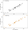 |
Fig. B.1 Comparison of envelope dust masses calculated with SCUBA (x-axis, COMPLETE survey, Ridge et al. 2006) and SCUBA-2 (y-axis, JCMT GBS, Kirk et al. 2018) data. The top panel shows the dust masses per source in our sample (i.e., APEX pointing), while the bottom panel shows the dust masses per system (i.e., summed masses of all components in multiple protostellar systems). |
With the aim to further check that our envelope dust masses are reasonable, we compare our SCUBA calculated values with the dust masses from the core catalog of Pezzuto et al. (2021). The core catalog was filtered to only consider cores classified as protostellar. By-eye coordinate matching was used to find a common sample of 35 cores for 31 systems in our sample. The match is not perfect since our work uses VANDAM survey positions (Tobin et al. 2016), while Pezzuto et al. (2021) used the getsources algorithm on Herschel PACS maps. This leads to different numbers of cores being associated with higher-order multiples in our sample; for example, NGC1333 SVS13 A, B, and C are associated with cores 314, 311, and 303 from Pezzuto et al. (2021), L1448 N A+B is associated with core 69, and L1448 N C is associated with core 68 from Pezzuto et al. (2021). From the matched sample, we find that 21 out of 35 cores have masses differing by a factor of 3 or less. In addition, 24 out of 35 cores present higher envelope dust masses in our sample than in the Pezzuto et al. (2021) core catalog. It should be noted that the core catalog employs SED fitting with a modified black body that is not suitable for protostellar sources (Pezzuto et al. 2021), while we use a method dependent on Lbol, distance and peak flux at 850μm (see Sect. 2.2 and Jørgensen et al. 2004). The largest discrepancies come from the adopted dust temperature in the SED fitting method and the luminosity obtained from integrating the SED LSED (Pezzuto et al. 2021). Core 311, corresponding to NGC1333 SVS13 B, does not have an SED fit in the core catalog. A dust temperature of 10.4 K (average of all reliable starless and prestellar SEDs) and LSED = 0.024 L⊙ is adopted for Core 311. Whereas we adopt a dust temperature of 20.79 K (Zari et al. 2016) and Lbol = 16.6 L⊙ (Murillo et al. 2016) for SVS13 B. For this case, the dust mass from Pezzuto et al. (2021) is 0.186 M⊙, while our dust mass is 2.87 M⊙, a factor of 15 difference and the largest discrepancy.
Appendix C APEX spectra
Samples of the Atacama Pathfinder Experiment (APEX) spectra for the extended sample (Project codes O-0104.F-9307A and O-0104.F-9307B, see Sect. 2.3 for additional details) used in this work are presented in this appendix. Figure C.1 shows spectra from three systems: a wide binary B1 Per6+Per10, a close binary L1455 Per17, and a single protostar NGC1333 RNO 15 FIR. Three molecular species with two transitions each are shown and were used to derive the physical parameters reported in this work: gas kinetic temperature from line peak ratios (see Sect. 4.1), column density (see Sect. 4.2), and gas masses (see Sect. 4.3). The comparison spectra of L1455 Per25 obtained from the observations of the pilot (Murillo et al. 2018a) and extended (this work) samples are shown in Fig. C.2. See Sect. 2.3 for more details.
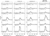 |
Fig. C.1 Sample of APEX spectra toward sources from the extended sample (see Sect. 2). The spectra for DCO+ J=5-4 and p-H2CO J=50,5-40,4 were obtained with APEX-2 with a beam of 18″, the other spectra were obtained with APEX-1 and a beam of 28.7″. From left to right, the first two panels show spectra for the components of the system B1 Per6+Per10. The third panel shows spectra for the close binary L1455 Per17. The fourth panel shows spectra for the single protostellar source NGC1333 RNO 15 FIR. The spectra are averaged to 0.4 km s−1 in order to increase sensitivity. All emission lines shown are found to have S/N ≥5 based on GILDAS/CLASS Gaussian fitting routines. |
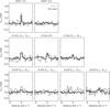 |
Fig. C.2 Comparison of spectra from the pilot (gray) and extended (black) samples for L1455 Per25. Both datasets were processed in the same manner and averaged to 0.4 km s−1. The molecular species shown are the same as listed in Table 1. The extended sample observations provide a better constraint for single protostars than the pilot observations. |
Sample of protostellar systems.
All Tables
All Figures
|
Fig. 1 Physical parameters derived from APEX observations. Top row : gas kinetic temperature and corresponding errors obtained from molecular line ratios. Cyan circles show the temperature obtained from DCO+ J=5-4/J=3-2, orange squares show the average temperature obtained from the three H2CO ratios, and black diamonds show the average temperature obtained from the two c-C3H2 ratios. Upper limits are indicated with a downward arrow. The horizontal dash-dotted red line indicates the average gas kinetic temperature (Tkin ~15 K) derived from the I(HCN)∕I(HNC) J =1-0 (Paper I). The gray crosses show the gas kinetic temperature from NH3 observations (Tkin,NH3) obtained from the core catalog of Rosolowsky et al. (2008). The left and right panels plot gas kinetic temperature versus bolometric luminosity (Lbol) and envelope dust mass (Menv), respectively. Bottom row : column density for DCO+ (cyan circles), H2CO (orange squares), and c-C3H2 (black diamonds) obtained from the respective lowest transition in the APEX data. Solid lines and shaded areas show the linear regression for the data with the corresponding color. The left and right panels plot column density versus Lbol and Menv. Error bars are smaller than the symbols. |
| In the text | |
|
Fig. 2 Gas mass (Mgas) versus dust mass (Menv) for all transitions of DCO+ (left panel), H2CO (center panel), and c-C3H2 (right panel). This plot shows that the gas masses from DCO+ and c-C3H2 are consistent between transitions, while H2CO shows a broader spread. In the center panel, the gas mass from H2CO 32,2-22,1 is not shown to avoid a crowded plot, but follows a similar distribution to the other transitions shown in the panel. |
| In the text | |
|
Fig. 3 Relations of the DCO+ J =1-0 gas mass (MDCO+, left column), H2CO J=30,3-20,2 gas mass (MH2CO, center column), and c-C3H2 J=33,0-22,1 gas mass (Mc-C3H2, right column) versus envelope dust mass (Menv) for the sample. In all panels the dash-dotted red line shows the N2H+ gas mass versus envelope dust mass from Paper I as reference. The full sample with no differentiation for multiplicity is shown in the top row. In the other three rows, orange stars indicate multiple protostellar systems, cyan diamonds show binary systems, and gray circles indicate single protostellar systems. Each row represents one of four ways of grouping the sample and their corresponding correlations (see Sect. 4.4). Lines and shaded areas show the linear regression for the data with the corresponding color. Solid lines indicate statistically significant correlations in the subsamples (censored Kendall rank correlation p value of <0.05), while the dashed line shows subsamples with p values of >0.05. |
| In the text | |
|
Fig. B.1 Comparison of envelope dust masses calculated with SCUBA (x-axis, COMPLETE survey, Ridge et al. 2006) and SCUBA-2 (y-axis, JCMT GBS, Kirk et al. 2018) data. The top panel shows the dust masses per source in our sample (i.e., APEX pointing), while the bottom panel shows the dust masses per system (i.e., summed masses of all components in multiple protostellar systems). |
| In the text | |
|
Fig. C.1 Sample of APEX spectra toward sources from the extended sample (see Sect. 2). The spectra for DCO+ J=5-4 and p-H2CO J=50,5-40,4 were obtained with APEX-2 with a beam of 18″, the other spectra were obtained with APEX-1 and a beam of 28.7″. From left to right, the first two panels show spectra for the components of the system B1 Per6+Per10. The third panel shows spectra for the close binary L1455 Per17. The fourth panel shows spectra for the single protostellar source NGC1333 RNO 15 FIR. The spectra are averaged to 0.4 km s−1 in order to increase sensitivity. All emission lines shown are found to have S/N ≥5 based on GILDAS/CLASS Gaussian fitting routines. |
| In the text | |
|
Fig. C.2 Comparison of spectra from the pilot (gray) and extended (black) samples for L1455 Per25. Both datasets were processed in the same manner and averaged to 0.4 km s−1. The molecular species shown are the same as listed in Table 1. The extended sample observations provide a better constraint for single protostars than the pilot observations. |
| In the text | |
Current usage metrics show cumulative count of Article Views (full-text article views including HTML views, PDF and ePub downloads, according to the available data) and Abstracts Views on Vision4Press platform.
Data correspond to usage on the plateform after 2015. The current usage metrics is available 48-96 hours after online publication and is updated daily on week days.
Initial download of the metrics may take a while.