| Issue |
A&A
Volume 704, December 2025
|
|
|---|---|---|
| Article Number | A154 | |
| Number of page(s) | 12 | |
| Section | Stellar atmospheres | |
| DOI | https://doi.org/10.1051/0004-6361/202554816 | |
| Published online | 12 December 2025 | |
Exploring stellar activity in a sample of active M dwarfs
1
Astronomy & Astrophysics Division, Physical Research Laboratory, Navrangapura,
Ahmedabad
380009,
India
2
I. Physikalisches Institut, Universität zu Köln,
Zülpicher Straße 77,
50937
Köln,
Germany
3
Center for Astrophysics | Harvard & Smithsonian,
60 Garden Street,
Cambridge,
MA
02138,
USA
4
Instituto de Astronomía, Universidad Católica del Norte,
Av. Angamos 0610,
Antofagasta,
Chile,
★ Corresponding authors: arvindr@prl.res.in; jose.fernandez@ucn.cl
Received:
28
March
2025
Accepted:
6
October
2025
Context. Most M dwarfs present high chromospheric activity that can exceed the solar magnetic activity. This can substantially influence planetary, atmospheric, and biological processes and might affect the habitability of orbiting planets. It is therefore important to characterize the magnetic activity of M dwarfs to understand the physical mechanisms that cause it. M dwarfs are the primary targets in the search for exoplanets within the habitable zone.
Aims. We characterize the stellar activity of active M dwarfs by understanding the relations between magnetic activities, stellar parameters, and flare properties.
Methods. We analyzed TESS photometric data combined with spectroscopic observations of active M dwarfs. We examined the relation between the flare occurrence rate, flare energies, rotation period, filling factor, and chromospheric activity indicators. Furthermore, we investigated the correlation between the flare amplitude and duration and the cumulative flare energy frequency distributions to probe the underlying mechanisms driving magnetic activity in flaring M dwarfs.
Results. The distribution of the flare occurrence rate is flat for spectral types M0–M4 (Teff ~ 3900–3200 K) and declines for later types. The flare occurrence rate and flare activity of faster rotators with Prot < 1 day is higher. M dwarfs with a higher flare occurrence rate tend to exhibit lower flare amplitudes, which indicates that the frequent flares in these M dwarfs are generally less energetic. Within the mass range of 0.15–0.76 M⊙, the median of LHα/Lbol in evenly divided mass bins of ~0.1 M⊙ varies by a factor of ~2.5, while ΔEW decreases by 92% across the sample. We derived power-law indexes of the cumulative flare frequency distribution for M dwarf subgroups that indicated a decreasing trend from M0 to M5 dwarfs with a value of α from 1.68 to 1.95, respectively.
Conclusions. We characterized the stellar activity in M dwarfs through chromospheric indicators such as the Hα emission, the starspot coverage, the flare occurrence rates, flare energies, and flare duration. Our results suggest a stellar activity transition near M4. Stronger Hα emission is linked to a higher flare occurrence. The flare occurrence rate of rapid rotators (Prot < 1 day) is significantly higher, which supports the idea that strong magnetic dynamos in fast-rotating M dwarfs sustain a frequent flaring activity. Our analysis confirms that highly active stars dissipate magnetic energy through numerous low-energy flares and not through a few high-energy events. We also show that chromospheric activity and flare activity follow a power-law relation.
Key words: techniques: spectroscopic / stars: activity / stars: atmospheres / stars: chromospheres / stars: flare / stars: low-mass
© The Authors 2025
 Open Access article, published by EDP Sciences, under the terms of the Creative Commons Attribution License (https://creativecommons.org/licenses/by/4.0), which permits unrestricted use, distribution, and reproduction in any medium, provided the original work is properly cited.
This article is published in open access under the Subscribe to Open model. Subscribe to A&A to support open access publication.
1 Introduction
M dwarfs are the coolest stars, with Teff ranging from 2500–4000 K, and the least massive (0.075–0.6M⊙) stellar objects in the Milky Way. They contribute roughly 40% of the total stellar mass (Henry 1998) and account for about 70% of the stellar population (Reid et al. 1995; Reylé et al. 2021). M dwarf populations show a broad range of evolutionary stages and chemical compositions, with young metal-rich M dwarfs in open clusters, while older metal-poor M dwarfs can be found in the Galactic halo (Green & Margon 1994). M dwarfs have gained particular interest in the search for habitable exoplanets. Luque et al. (2022); Kossakowski et al. (2023), and Donati et al. (2023, 2024) reported exoplanets orbiting M dwarfs. Klein et al. (2022) discovered exoplanets around the bright young active M-dwarf AU Mic, and Anglada-Escudé et al. (2016) reported a terrestrial planet around the nearest M dwarfs to the Sun, Proxima Centauri.
Various optical and near-infrared (NIR) observational facilities such as High Accuracy Radial velocity Planet Searcher (HARPS) (Mayor et al. 2003; Cosentino et al. 2012), CRyogenic high-resolution InfraRed Echelle Spectrograph (CRIRES) (Kaeufl et al. 2004), Calar Alto high-Resolution search for M dwarfs with Exoearths with Near-infrared and optical Echelle Spectrographs (CARMENES) (Quirrenbach et al. 2014), SPectropolarimetre InfraROUge (SPIRou) (Cersullo et al. 2017), HPF (Mahadevan et al. 2012), and Near-InfraRed Planet Searcher (NIRPS) (Bouchy et al. 2025) have started to yield high-quality spectra with a high signal-to-noise ratio. These high-quality spectra offer a powerful tool for investigating the properties of M dwarfs, such as their fundamental parameters and radial velocities, which enable the detection of low-mass exoplanets (Astudillo-Defru et al. 2017; Amado et al. 2021). Further, it allows us to determine their elemental abundances, line broadening, and Zeeman splitting in magnetically sensitive lines, which offer constraints on their rotation.
The active nature of M dwarfs substantially affects the atmosphere of planets that orbit them through the high-energy radiation they receive, which in turn affects their potential habitability (Tilley et al. 2019). Compared to hotter stars like our Sun, M dwarfs are known to be more active. West et al. (2004) suggested that the fraction of active M dwarfs increases from M0 to M8 and then in later spectral types, particularly in the brown dwarf (L3-L4) regime. The magnetic activity can generate variability in radial velocity (RV) measurements, often mimicking periodic signals similar to those caused by actual exoplanets. To assess the habitability of exoplanets orbiting these stars, the evolution of planetary systems in general, and to explore various physical mechanisms underlying these signals generated by stellar activity, it is therefore necessary to understand the magnetic activity of M dwarfs.
Spectroscopic and photometric tools have been used quite extensively to study stellar activity in M dwarfs. Various spectral lines such as Mg II, Ca II, Na I, K I, and Hα are widely used to assess the chromospheric activity within the optical spectral range, which covers the temperature minimum region to the upper chromosphere (Cincunegui et al. 2007; Díaz et al. 2007; Cao & Gu 2014). The variations in the mean line-core flux of these lines can then be used to indicate the overall activity level of M dwarfs. Flux variations in these lines provide valuable insights into the different regions within the stellar atmosphere at varying heights. For instance, the Hα emission line forms in the upper chromosphere, Na I lines originate in the lower chromosphere, and Ca II and K I lines span from the middle chromosphere to the upper chromosphere (Mauas & Falchi 1994; Leenaarts et al. 2012; Fontenla et al. 2016).
One method of probing the stellar activity is to investigate flares and to use them as a proxy for magnetic activity. Flares are short-lived but powerful energetic phenomena that occur on main-sequence stars, where magnetic energy is converted into transient emissions spanning a broad spectrum of wavelengths from radio to X-rays. These events also drive plasma heating, particle acceleration, and large-scale plasma motion. (Benz & Güdel 2010; Crowley et al. 2024). Shibayama et al. (2013) suggested that stellar flares follow the power-law relation ![$\[\frac{d N}{d E} \propto E^{-\alpha}\]$](/articles/aa/full_html/2025/12/aa54816-25/aa54816-25-eq1.png) with α ~ 2. These flares are thought to result from a magnetic reconnection event, which produces a beam of charged particles that collide with the stellar photosphere. This interaction triggers intense heating and emits radiation across nearly the entire electromagnetic spectrum (Davenport 2016). During the flare, magnetic reconnection is thought to cause a change in the field line topology that leads to a significant energy release, often on the order of the magnitude of X-class solar flares or even greater (Pettersen & Hawley 1989; Doyle et al. 2018). The flare timescales in stars are also unpredictable. They can range from a few hours to a few days. A systematic sample of flares for an individual star is therefore a highly resource-demanding venture and was performed for only a few particularly active stars.
with α ~ 2. These flares are thought to result from a magnetic reconnection event, which produces a beam of charged particles that collide with the stellar photosphere. This interaction triggers intense heating and emits radiation across nearly the entire electromagnetic spectrum (Davenport 2016). During the flare, magnetic reconnection is thought to cause a change in the field line topology that leads to a significant energy release, often on the order of the magnitude of X-class solar flares or even greater (Pettersen & Hawley 1989; Doyle et al. 2018). The flare timescales in stars are also unpredictable. They can range from a few hours to a few days. A systematic sample of flares for an individual star is therefore a highly resource-demanding venture and was performed for only a few particularly active stars.
Low-mass stars, particularly M dwarfs with the deepest convective zones, flare more frequently than G or K dwarfs (Walkowicz et al. 2011). In mid- to late-M dwarfs, the occurrence rate of flares is nearly 30%, and in early-M dwarfs, it is 5% and lower than 1% for stars with F, G, and K spectral types (Günther et al. 2020). During the flare, the released energy ranges from 1029 to 1032 erg (Parnell & Jupp 2000; Shibayama et al. 2013). Fast-rotating M dwarfs flare more frequently. These fast-rotating M dwarfs with a rotation period (Prot) < 10 days vary significantly in their light curves, possibly due to starspots, which are thought to be imprints of magnetic field lines on their photosphere. Ramsay et al. (2013), Davenport et al. (2014), and Doyle et al. (2018) presented evidence that challenged this view, however. They observed no correlation between the number of flares, their amplitudes, and the rotational phase in M dwarfs that were studied with Kepler and K2. This suggests that flares may occur independently of a large dominant starspot. In slow-rotating M dwarfs, the ratio of X-rays, Hα, and CaH & K flux to the bolometric luminosity also declines rapidly, whereas the activity remains saturated for fast rotators (Raetz et al. 2020). In fast-rotating M dwarfs, large spots might also exist and are probably located randomly on the surface at a very short length scale (Magaudda et al. 2020).
Photometric surveys, including Kepler, its successor K2 (Howell et al. 2014), and the Transiting Exoplanet Survey Satellite (TESS) (Ricker et al. 2015), have significantly increased interest in studying magnetic phenomena in host stars because they affect exoplanets. These surveys observe large samples with high photometric precision, enabling the detection of magnetic activity indicators such as flares, periodic luminosity variations (Reinhold et al. 2017), and starspot variability, which helps us to identify stellar activity cycles. Using the high-precision photometry from the Kepler survey Maehara et al. (2012), we found many energetic superflares, which are even 104 times larger than solar flares. Based on these high-precision photometric data, strong correlations between the flare energy, amplitude, duration, and decay time were reported by Hawley et al. (2014); Raetz et al. (2020), and Yang et al. (2023). The contrast between flares and the quiescent state of a star is also more prominent in M dwarfs, which led to fewer studies on flares in field G dwarfs. For inactive stars like our Sun, the flare rates are highly unconstrained.
The primary objective of this study is to investigate stellar flares and magnetic activity in M dwarfs through combined spectroscopic and photometric observations. In particular, we examine the relation between flare properties such as flare activity (Lflare/Lbol), flare energy ⟨Eflare⟩, flare frequency, and flare occurrence rate (FOR) and various stellar activity indicators, including Hα activity strength (LHα/Lbol), spectral type, Prot, flare frequency distribution (FFD), and starspot-filling factor (fs). Section 2 presents the target sample along with spectroscopic and photometric observations. Section 3 describes the methods we used to analyze the chromospheric activity and flare parameters. The results and their implications are discussed in Section 4, and our conclusions are given in Section 5.
2 Data
2.1 Target sample
In this current study, our sample consisted of bright field active M dwarfs with spectral types ranging from M0 to M8.5. They were selected from the catalog of Kumar et al. (2023). The majority of M dwarf targets in our sample lie on the main sequence, and only a small fraction has pre-main-sequence ages based on the StarHorse ages (Queiroz et al. 2018; Anders et al. 2019) reported by Kumar et al. (2023). The targets in our sample lie at intermediate to high Galactic latitudes (typically |b| ≳ 15–20°), well away from the Galactic plane. This minimizes the likelihood of contamination from young stellar associations. Fig. 1 shows the distance distribution and the TESS magnitude distribution of all the stars in our sample. The distances and TESS magnitudes were taken from Stassun et al. (2018).
2.2 Spectroscopic activity parameters
In our previous work (Kumar et al. 2023), we conducted low-resolution (R~1000) spectroscopic monitoring of active M dwarfs (M0–M6.5) using the Mount-Abu Faint Object Spectrograph and Camera- Pathfinder (MFOSC-P) (Srivastava et al. 2018, 2021; Rajpurohit et al. 2020). The spectrograph covers the spectral range of 4700–6650Å. Kumar et al. (2023) focused on the variability in the Hα and Hβ emission lines over timescales ranging from ~0.7 to 2.3 hours, with a cadence of approximately 3–10 minutes. In this study, we analyzed a total of 126 M dwarfs in the spectral range of M0-M8.5. All the M dwarf sources we used are strongly chromospherically active, as indicated by the Hα equivalent widths, which are shorter than −0.75 Å. This is consistent with prominent Hα emission (Kumar et al. 2023). For further details regarding the data reduction, we refer to Kumar et al. (2023).
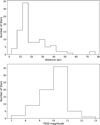 |
Fig. 1 Distance distribution (top panel) of stars in our sample, binned at 5 pc intervals, and the TESS magnitude distribution (bottom panel) of the same sample. |
2.3 TESS photometry
2.3.1 Obtaining high-cadence data
TESS is a dedicated mission to monitor approximately 200 000 bright stars distributed across the sky. NASA launched TESS in April 2018. TESS observes in the spectral interval of 6000–10000 Å, encompassing the blue optical to near-infrared regions. TESS satellites have provided unprecedented data with available 2-minute cadences for various stellar sources (Ricker et al. 2015). We used TESS short-cadence photometric data for the active M dwarfs in our sample. These high-cadence photometric data enabled us to determine the Prot, FOR, flare energies, and fs of the M dwarfs. Using the Python package lightkurve1, we efficiently retrieved the light curves for these stars. The number of sectors per target ranges from one to ten. Complete sector lists along with TESS magnitudes and distances are provided in Appendix A.1. Twelve of 126 M dwarfs from our sample were excluded from this study because 5 lacked TESS data and 7 had no reliable light curves. For further details on the method and the determination of Prot and fs, we refer to Kumar et al. (2023).
2.3.2 Quality checks and contamination
For quality checks and contamination, we analyzed 114 out of 126 M dwarfs from our sample that were observed by TESS between 2018 and 2024 in multiple sectors and epochs. For consistency, we restricted our analysis to the light curves processed by the Science Processing Operations Centre (SPOC) (Jenkins et al. 2016) and TESS-SPOC (Caldwell et al. 2020) pipelines, adopting the presearch data-conditioning simple-aperture photometry (PDCSAP) flux. High-cadence observations with integration times of 20, 120, 200, and 600 seconds are available for subsets of the targets and were used in this study. For each target, we used all available TESS sector light curves for the analysis, as provided in Appendix A.1. To quantify flux contamination from neighboring sources, we employed TESSILATOR2, which computes the total neighbor-to-target flux ratio (Ση) (for more details, see Binks & Günther 2024). Targets with Ση > 0.3 were classified as contaminated and excluded from the flare analysis. Using this criterion, we identified 8 of 114 targets as contaminated and removed them from the final sample.
3 Methods and analysis
3.1 Flare detection using photometric data from TESS
Numerous algorithms for automated flare detection have been developed (Walkowicz et al. 2011; Davenport 2016; Gao et al. 2016), and several methods have been applied to systematically identify and characterize these events in photometric light curves (Feinstein et al. 2020; Yang et al. 2023; Meng et al. 2023). We employed the Altaipony3 Python package (Ilin, Ekaterina et al. 2021; Davenport 2016) for the automated identification and analysis of flares within stellar light curves.
In the Altaipony module, the de-trending of light curves was initially performed with a Savitzky-Golay filter (Savitzky & Golay 1964) to remove long-term trends. Then, the flare detection algorithm was employed using the Altaipony package. As outlined by Chang et al. (2015), flares were identified based on the three key parameters N1, N2, and N3 within the Altaipony package. A candidate event was classified as a flare only when the following criteria were satisfied: (1) it deviated positively from the median quiescent flux of the star, where the flux deviation at a given data point exceeds the local scatter in the light curve by N1=3 times, (2) the combined deviation and flux error exceed the local scatter by N2=3 times, and (3) at least N3=3 consecutive data points satisfied the N1 and N2 thresholds.
Using this approach, we identified 94 flaring objects out of 106 M dwarfs observed with TESS. The complete lists of flaring and nonflaring stars are given in Appendices A. 1 and A.2. To quantify the robustness of our flare detections, using AltaiPony, we performed injection–recovery tests on the 20-s cadence TESS light curve of 2MASSWJ1012065-304926, an M6.0 star with a TESS magnitude of 14.5. We recovered 51 out of 58 injected synthetic flares. This corresponds to an overall completeness of 90%, and the missed detections were confined to the lowest-amplitude events. Our analysis with AltaiPony confirms the reliability of detecting moderate to strong flares, even in cases with the lowest S/N in our sample, with a false-positive rate <5%. During the analysis, a visual inspection was also conducted by generating plots of flare candidates overlaid on the stellar background for each light curve. This provided an additional verification. Figure 2 illustrates the smoothed photometric light curve we obtained during the detrending process, where a Savitzky–Golay filter with a window length of 0.1 days and a second-order polynomial fit was applied. The quasi-sinusoidal brightness variations observed in PM J16170+5516 (M2.0) are visible, and we attribute them to the rotational modulation caused by prominent starspots that come into and rotate out of view, as captured in the TESS data (Ricker et al. 2015).
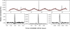 |
Fig. 2 Top panel: TESS light curve of PM J16170+5516 (M2.0) from Sector-25, 2020 (SPOC) with Prot 1.975 days. The black line shows the light curve with a cadence of 2 min, and the red line represents the Savitzky–Golay filtered and smoothed curve. Bottom panels: zoomed views of the detrended flux highlighting multiple flare events of different magnitudes. |
3.2 Estimating the flare energy
M dwarfs are known for their frequent and energetic flaring activity. These transient events are associated with their fully convective envelopes, particularly in late-type stars with spectral types ranging from M3 to M9 (Reiners et al. 2012; Newton et al. 2017). The flare energy is a critical parameter for quantifying the magnetic activity of stars. We calculated the energy of each flare following the method established by Shibayama et al. (2013) and Yang et al. (2017), using stellar luminosity, flare duration, and flare amplitude. Under the assumption that flaring M dwarfs act as blackbody radiators with an effective temperature of Tflare = 9000 K, as proposed by Kretzschmar (2011), the bolometric flare luminosity at a given time during the flaring event Lflare,i was computed as
![$\[L_{\text {flare}, i}=\sigma T_{\text {flare}}^4 A_{\text {flare}, i},\]$](/articles/aa/full_html/2025/12/aa54816-25/aa54816-25-eq2.png)
where σ denotes the Stefan–Boltzmann constant, and Aflare,i represents the flare area and is determined by the relation
![$\[A_{\text {flare}, i}=C_{\text {flare}, i} ~\pi R^2 \frac{\int R_\lambda B_\lambda\left(T_{\text {eff}}\right) \mathrm{d} \lambda}{\int R_\lambda B_\lambda\left(T_{\text {flare}}\right) \mathrm{d} \lambda},\]$](/articles/aa/full_html/2025/12/aa54816-25/aa54816-25-eq3.png)
![$\[C_{\text {flare}, i}=\frac{F_i-F_o}{F_o}.\]$](/articles/aa/full_html/2025/12/aa54816-25/aa54816-25-eq4.png)
In this formulation, Rλ is the TESS response function4, Bλ(T) is the Planck function at temperature T, R is the stellar radius, Fi is the measured flux at a given time during the flare event, and Fo is the quiescent flux (at the same time) of the star. The stellar radii were taken directly from the TESS input catalog (TIC) and candidate target list (CTL) when available (Stassun et al. 2018) and are tabulated in Appendix A.1. The total bolometric energy of a flare was then obtained by integrating Lflare,i over the whole duration of the flare, whereas the flare duration was determined using the Altaipony algorithm. The uncertainties in the flare energy estimations are significant. Shibayama et al. (2013) reported an approximate error margin of ±60%. The estimated stellar radius and the average flare energy ![$\[\left\langle E_{\text {flare }}\right\rangle=\frac{1}{N} \sum_{i=1}^{N} E_{i}\]$](/articles/aa/full_html/2025/12/aa54816-25/aa54816-25-eq5.png) , and Lflare/Lbol are tabulated in Appendix B.1.
, and Lflare/Lbol are tabulated in Appendix B.1.
3.3 Flare occurrence rate, flare duration, and flare amplitude
We also examined the relation between the Prot and the FOR in our sample of M dwarfs. For sources with flare episodes, the FOR was calculated as the ratio of the total duration of all flaring events to the total observing duration defined by Walkowicz et al. (2011),
![$\[\mathrm{FOR}=\frac{\sum t_{\text {flare }}}{\sum t_{\text {star }}} \times 100,\]$](/articles/aa/full_html/2025/12/aa54816-25/aa54816-25-eq6.png)
where ∑tflare is the summation of the flare duration of each star, and ∑tstar is the observation period of each star. The flare duration was determined using the Altaipony algorithm, and the observation period was estimated by multiplying the exposure time of each data point by the total number of data points searched for flare epochs in the detrended light curve.
The flare amplitude is also a key parameter in defining the characteristics of a flare event. To understand the flare amplitude statistics in the spectral range in our sources, the flare amplitude was determined for each flare using the Altaipony algorithm, which measures the difference in flux at the peak of the flare relative to the quiescent stellar flux. The FOR and median flare amplitude for each source are tabulated in Appendix B.1.
Summary of TESS observations, flaring sources, and FFD parameters.
3.4 Flare frequency distribution
As flares span a wide energy range, cumulative flare frequency distributions (FFDs) are commonly used to describe the occurrence of flares as a function of energy (Hawley et al. 2014; Davenport 2016; Ilin, Ekaterina et al. 2021; Jackman et al. 2021). The cumulative flare frequency ν ~ (>E) for a given flare energy E is determined by the total number of flares with flare energy ≥E, divided by the total observation duration of the target. The FFDs follow power-law relations and are written as
![$\[\mathrm{d} N(E)=k E^{-\alpha} \mathrm{d} E,\]$](/articles/aa/full_html/2025/12/aa54816-25/aa54816-25-eq7.png)
where N is the number of flares that occur in the total observation duration, E is the flare energy, k is a proportionality constant, and α is the power-law index. Thus, the flare frequency (ν) can be estimated by integrating the above equation,
![$\[\log~ \nu=\log \left(\frac{k}{1-\alpha}\right)+(1-\alpha) ~\log~ E.\]$](/articles/aa/full_html/2025/12/aa54816-25/aa54816-25-eq8.png)
The parameter α determines the relative occurrence of high-energy flares compared to lower-energy ones and has been found to vary across different spectral types. Previous studies have shown that α is negative, indicating that high-energy flares are less frequent than their low-energy counterparts (Shibayama et al. 2013).
The low-energy regime of FFDs is often incomplete because not all low-energy flares are recovered (Davenport 2016). This incompleteness can be noted as a deviation from the expected power-law behavior and appears as a flattening in log-log space at lower energies. The detection method becomes less sensitive at these low energies, resulting in an underestimation of flare detections. To mitigate this effect, many studies restricted their analysis to flare energies above a certain threshold, well beyond the turnover, to ensure a more reliable power-law fit (Hawley et al. 2014). Following the same approach, we also restricted the data for the power-law fitting to the energy of 1032 ergs (see Table 1 for more details). Section 4.3 examines the FFDs of M dwarfs by categorizing them based on spectral type using this power-law approach.
4 Results and discussion
4.1 Hα variability
Various observable phenomena that occur in the outer stellar atmosphere, such as strong stellar winds, flares, coronal mass ejections, and starspots, are generally used to characterize the magnetic activity in stars. These processes give rise to distinct chromospheric emission lines, among which the Hα emission line is widely used for activity-related studies, particularly in M dwarfs. The investigation of the short-term variability of Hα emission line properties provides valuable insight into these magnetic processes. The statistical properties of Hα equivalent width and LHα/Lbol were previously analyzed by Kumar et al. (2023) by spectroscopic monitoring for a sample of M dwarfs (for a detailed discussion of the estimation methods and statistical analysis of these parameters, we refer to Kumar et al. 2023). We used these properties to determine a plausible relation between chromospheric activities and the flare phenomenon.
Figure 3, as an example, shows various temporal spectra from different observations of the flaring M dwarf PM J12142+0037, which is spectral type M4. The temporal changes in the Hα emission since the beginning of the first exposure are evident. This enhanced emission of Hα is generated through collisional excitation within the relatively dense chromosphere and is the most prominent and commonly used indicator of stellar magnetic activity. This temporal variation in the Hα emission line might be linked to the emergence of active regions on the stellar surface.
4.2 Chromospheric activity as a function of mass
Gomes da Silva et al. (2011) and Robertson et al. (2013) suggested that magnetic activity is higher in massive M dwarfs than in their lower-mass counterparts. Notably, Robertson et al. (2013) proposed that compared to either effective temperature (Teff) or stellar color, the stellar mass serves as a better predictor of the mean Hα activity. The relation between chromospheric activity and mass in M dwarfs is more complex than in massive stars. Some correlation between chromospheric activity and mass might still exist within the M dwarf population, however.
To explore the possibility of any correlation between chromospheric activity strength and stellar mass among flaring M dwarfs in our sample, we adopted the stellar masses provided by Stassun et al. (2018). They were derived using the MKs–mass relation from Mann et al. (2015) and Benedict et al. (2016). In the top panel of Figure 4, we display the distribution of ΔEW = max(EW) – min(EW) for the Hα emission as a function of seven equally spaced mass bins. Our analysis shows that for the lower-mass regime M⊙ < 0.2, the scatter in Hα is larger, but decreases steadily at higher masses M⊙ > 0.35. The bottom panel of Figure 4 shows the distribution of the median values of LHα/Lbol as a function of stellar mass, where the scatter in each bin is quantified using the median absolute deviation (MAD), scaled by 1.48 for consistency (Mazeh et al. 2015). The uncertainty in the median for each bin is estimated as ![$\[\frac{\text {MAD}}{\sqrt{N}}\]$](/articles/aa/full_html/2025/12/aa54816-25/aa54816-25-eq9.png) , where N represents the number of data points within the bin. LHα/Lbol peaks nearly at ~0.2–0.3 (M⊙) and then becomes nearly flat beyond ~0.3 M⊙. The ΔEW decreases by approximately 92%, spanning a factor of about 6.3 times above and below the linear fit. This variation indicates that despite their long activity lifetimes, the chromospheric heating efficiency in the coolest M dwarfs is reduced. This indicates that chromospheric activity across the mass range of ~0.2–0.3 (M⊙) might be attributed to the transition to fully convective interiors Reiners et al. (2012); West et al. (2015); Newton et al. (2017). These changes induce fundamental changes in the processes that generate strong magnetic fields in M dwarfs. The limited sample size prevents us from drawing firm conclusions, however. Nevertheless, we infer that the variability in the chromospheric Hα emission is positively correlated with stellar mass. This is consistent with the findings of Robertson et al. (2013); Lin et al. (2019), and Günther et al. (2020).
, where N represents the number of data points within the bin. LHα/Lbol peaks nearly at ~0.2–0.3 (M⊙) and then becomes nearly flat beyond ~0.3 M⊙. The ΔEW decreases by approximately 92%, spanning a factor of about 6.3 times above and below the linear fit. This variation indicates that despite their long activity lifetimes, the chromospheric heating efficiency in the coolest M dwarfs is reduced. This indicates that chromospheric activity across the mass range of ~0.2–0.3 (M⊙) might be attributed to the transition to fully convective interiors Reiners et al. (2012); West et al. (2015); Newton et al. (2017). These changes induce fundamental changes in the processes that generate strong magnetic fields in M dwarfs. The limited sample size prevents us from drawing firm conclusions, however. Nevertheless, we infer that the variability in the chromospheric Hα emission is positively correlated with stellar mass. This is consistent with the findings of Robertson et al. (2013); Lin et al. (2019), and Günther et al. (2020).
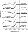 |
Fig. 3 Temporal variation in the Hα line profiles for PM J12142+0037 (M4.0) since the beginning of the first exposure. The dashed lines indicate the pseudo-continuum regions. The equivalent widths are marked to the left of each emission line, and elapsed times since the initial exposure are shown on the right. |
4.3 Flare energies, flare duration, and flare frequency distribution
As discussed in Section 3.1, 95 M dwarfs out of 106 sources observed by TESS exhibit flare episodes. The flare duration, amplitude, and energies were estimated for these sources. In Figure 5 we show the distribution of flare-event duration, suggesting that ~65–86% of the flares last for less than 10 minutes, and only very few (~2–4%) flaring events last more than 60 minutes. Short-duration flares (<10 minutes) are significantly more common in M dwarfs than long-duration flares (>10 minutes). This trend is evident for all spectral subtypes of M dwarfs, and later-type M dwarfs (M4-M6.5) have the highest relative frequency of short-duration flares. The common nature of these rapid flares suggests that magnetic reconnection events in M dwarfs often result in impulsive energy releases, likely affected by their fully convective nature and strong magnetic activity. Additionally, this high incidence of short-duration flares is closely linked to the rapid rotation rates of M dwarfs as it enhances the stellar activity by increasing the dynamo efficiency, which leads to more frequent and shorter-duration flares (Newton et al. 2017; West et al. 2015; Lin et al. 2019; Günther et al. 2020). Observational studies from Kepler, TESS, and K2 showed that the majority of detected flares in M dwarfs are short, and only a small fraction persists beyond ~20 minutes (Davenport et al. 2014; Hilton et al. 2010; Raetz et al. 2020). The decline in longer-duration flares in all subtypes implies that large-scale energy storage and release events are less frequent. Our results are consistent with the fact that magnetic reconnection events in M dwarfs are affected by the stellar structure. Fully convective stars (M4 or later) flare more frequently but shorter than partially convective stars (M0–M3). The details of flaring sources, number of flares, and flare percentage with tflare < 10 minutes are tabulated in Table 1.
Based on TESS, Kepler, and K2 data, various previous studies (Shibayama et al. 2013; Davenport 2016; Lin et al. 2019; Zhang et al. 2020) found that the flare energy ranges between ~1 × 1033 and 1 × 1036 ergs with an upper limit of 1 × 1038. Based on TESS data, the study by Doyle et al. (2019) found that flare energies in M dwarfs range from 6 × 1029 to 2.4 × 1035 ergs, whereas Günther et al. (2020) reported that the flare energy ranges from 1 × 1031 to 1038. As suggested by Yang et al. (2023), we also found that there is a clear boundary at about 1035 erg, and the flare energies of our M dwarf stars are lower than 1035 erg. The estimated average energy, that is, the average energy per flare ⟨Eflare⟩ for each source, is tabulated in Appendix B.1. The relation between the flare energy and flare duration for different M subspectral types is plotted in Figure 6. The dashed lines represent the power-law fit. The value of α lies between approximately 0.505 and 0.621, indicating that higher-energy flares generally last longer. We attribute the variation in α in the spectral types to the different magnetic field structures and their different convective nature. Our findings are consistent with studies that examined the rotation-activity relations and flare characteristics of M dwarfs (Lin et al. 2019; Doyle et al. 2019; Yang et al. 2023).
Based on all the flare energies in our analysis for the stars, the FFDs for the flare energies can better describe the behavior of flare activity in stars. We computed the FFDs for M dwarfs, categorizing them into spectral subgroups, as explained in Section 3.4. In Figure 7 we present the cumulative flare frequency distribution of flaring M dwarfs of different M subspectral types overlaid with a power-law fit (dashed line). For the M6–M6.5 sample (last panel), no power-law fit is shown because there were too few flares. We restricted our power-law fitting for all spectral type bins to flares with energies above 1032 following the approach of Hawley et al. (2014). The coefficient α, as described in Section 3.4, provides insight into the stellar flare activity. α is ~1.68 for M0-M0.5, whereas for M5-M5.5, α is ~1.95. This indicates that the distribution of the flare energies changes systematically from earlier to later spectral types. The figure clearly shows that low-energy flares dominate the overall distribution, while high-energy flares become progressively rarer. The slightly steeper slopes for M dwarfs M4 to M5 might also be due to a larger contribution from low-energy flares. The dependence of α in the spectral subtypes suggests that the underlying flare generation mechanism is broadly coherent (Lin et al. 2019).
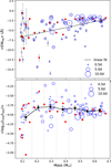 |
Fig. 4 Variability and activity indicators as a function of stellar mass. Top panel: Distribution of ΔEW = max(EW) – min(EW) for Hα emission. The dashed black line shows a linear fit, ΔEWHα = a(M*) + b, with a = 7.71 ± 1.55, b = −7.38 ± 0.64. Bottom panel: Median values of log10(LHα/Lbol) for Hα emission as a function of stellar mass. The black squares mark the medians in seven equally spaced bins with scatter quantified using the median absolute deviation. The blue circles are scaled by Prot, and larger circles correspond to longer Prot. The filled red circles indicate stars without a measured rotation period. The vertical gray lines show the bin sizes. |
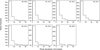 |
Fig. 5 Distribution of flare durations for M dwarfs (in minutes) shown for spectral subtypes M0–M6.5. |
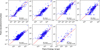 |
Fig. 6 Flare energy–duration relation for M dwarfs. The dashed red line shows the power-law fit (see Section 3.4). |
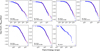 |
Fig. 7 Cumulative flare frequency distribution for M dwarfs plotted as a function of flare energy for the spectral types. The dashed red line shows the power-law fit (see Section 3.4). For the M6–M6.5 sample, no fit is shown because there were too few flares. |
4.4 Relation of FOR with Teff, Prot, and flare amplitude
Stellar flares occur spontaneously and are difficult to predict. In M dwarfs, the detection of flares is very challenging because of their sporadic nature and the observational limitations of ground-based telescopes. The FOR values vary in the spectral types, reach their peak in stars with strong magnetic dynamos, and decrease in those with weaker magnetic fields. Compared to G and K dwarfs, cooler M dwarfs sustain more active dynamos, leading to a higher FOR during their early fast-rotation stages.
Figure 8 presents the relation between Teff and FOR. Our analysis shows that FOR increases with Teff up to ~3200 K, above which it increases slowly. This observed rise in FOR in M dwarfs with Teff is consistent with the fact that hotter M dwarfs (M0-M4) have stronger magnetic and chromospheric activity than cooler M dwarfs (M4 or later). As suggested by Meng et al. (2023), lower-intensity flares are also more easily detected against the lower continuum of cooler M dwarfs. Our results might not be statistically significant because the number of flaring stars in the spectral range M5-M9 is limited, and we need more M dwarfs in this spectral range. Nevertheless, our findings agree with previous studies by Lin et al. (2019); Stelzer et al. (2022) and Yang et al. (2023).
Stellar rotation plays a critical role in determining the flaring activity of M dwarfs. It is one of the essential parameters that affect flare events. In general, faster-rotating M dwarfs exhibit significantly higher FOR than slower rotators (Wright et al. 2011; Notsu et al. 2013; Candelaresi et al. 2014; Yang et al. 2023). Since all M dwarfs in this study have measurable starspots indicative of strong magnetic activity, they were observed to produce flares from TESS light curves. We used the Prot derived by Kumar et al. (2023). The sample comprises fast-rotating M dwarfs with Prot < 10 days. The Prot were grouped into bins, and Prot of each bin was used for the analysis. The uncertainty in the median was calculated as explained in Section 4.2. It is important to note that individual TESS sectors span approximately 27 days, which limits the sensitivity of the period detection to roughly 10 days or shorter.
In Figures 9 and 10, we explore the relation between the Prot with FOR and flare amplitude. The Prot of M dwarfs in our sample range from 0.12 to 10.5 days. Figure 9 shows that FOR remains constant across the Prot < 10 days. Although the individual stars show larger scatter, in the binned averages, FOR does not depend significantly on Prot. We infer that this behavior might arise from their efficient dynamos, which can sustain frequent flaring activity in the fast-rotating (Prot < 10 days) M dwarfs. While our findings agree with previous studies, including Lin et al. (2019) and Yang et al. (2023), we note that our sample is limited to fast-rotating M dwarfs with Prot < 10 days. Further investigation is needed to explore whether this behavior persists in M dwarfs with FOR in M dwarfs with Prot > 10 days.
In Figure 10 we show the median of the peak flare amplitudes (AMed) of all flare events for each source versus FOR. The flare median amplitudes are usually found to be smaller and in the range of 0.01–1.0, and the flare amplitudes are independent of stellar rotations. We also found a negative correlation between FOR and flare amplitude. The reason might be that M dwarfs with higher FOR tend to exhibit lower flare amplitudes, indicating that frequent flares in these M dwarfs are generally less energetic (Raetz et al. 2020). More active stars might also release their magnetic energy in smaller frequent bursts, whereas less active stars accumulate magnetic energy over longer periods, which leads to rarer but more powerful flares (Stelzer et al. 2016; Yang et al. 2023; Günther et al. 2020).
Several theoretical models and observational studies have established a strong correlation between stellar flares and chromospheric activity. The Hα emission line, which is highly sensitive to magnetic field strength and Prot, is a key diagnostic of chromospheric activity and is closely linked to flare mechanisms (Chang et al. 2017; Zhang et al. 2020). We examined the connection between FOR and chromospheric activity indicators to explore this relation further, specifically, the Hα equivalent width (EW) and its variability, Δ(Hα EW), as illustrated in Figure 11. Our analysis revealed a slightly negative correlation between Hα EW and Δ(Hα EW) as a function of FOR, with M dwarfs exhibiting larger Hα EW and Δ(Hα EW) tending to have higher FOR. Strong and variable Hα emission suggests an actively heated chromosphere, driven by underlying magnetic fields, which contributes to frequent and energetic flaring activity (Doyle et al. 2019; Lin et al. 2019). The M dwarfs in this study predominantly exhibit Prot < 10 days, and their high FOR can therefore be attributed to rapid rotation, which amplifies their magnetic dynamo efficiency and sustains heightened magnetic activity (Newton et al. 2017).
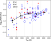 |
Fig. 8 FOR vs. Teff for M dwarfs. The black squares show the median values in five equally spaced bins. The symbols have the same meaning as in Fig. 4. |
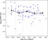 |
Fig. 9 FOR as a function of Prot. The blue circles represent individual stars. The black square marks the median values in five equally spaced bins on a log scale. The error bars on the medians are discussed in Section 4.2. |
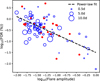 |
Fig. 10 Flare amplitude vs. FOR. The dashed line shows the best-fit power law, FOR = k (flare amplitude)α, where k = 0.032 ± 0.01 and α = −0.8 ± 0.09. The symbols have the same meaning as in Fig. 4. |
4.5 Flare activity. Quantification
According to the stellar dynamo theory, the interaction between stellar rotation and convection drives the generation of magnetic fields. The stellar chromospheric activity is closely linked to the rotation period. Noyes et al. (1984) studied the effect of these two factors on magnetic dynamo efficiency and combined them into a single parameter known as the Rossby number.
In Figure 12 we present the relation between Lflare/Lbol and the Prot. As expected for M dwarfs, the trend is similar, where there is a decline in Lflare/Lbol as Prot increases. In our analysis, unlike traditional saturation observed in other activity indicators as shown by Yang et al. (2017), this saturation is not observed because we lack M dwarfs with Prot > 10 days.
The relation between Lflare/Lbol and Teff is depicted in Figure 13. The flare activity for early-type M dwarfs (M0-M4) with Teff > 3200 K remains relatively stable at ~5 × 10⁻³. In contrast, a rapid increase of nearly an order of magnitude in the average flare activity is observed for M dwarfs with Teff < 3200 K, indicating the disappearance of low-activity flaring stars at cooler Teff. At the same Teff, stars with shorter Prot generally exhibit stronger flare activities. We would like to mention, however, that the overall number of M dwarfs with Teff < 3200 K is much smaller than in other warmer Teff bins.
In active stars, the Hα emission line is highly affected by the magnetic fields and Prot, which play a crucial role in the flare mechanism. As LHα/Lbol and Lflare/Lbol also serve as a proxy for stellar activity, it is very useful to examine the relation between them. We therefore also attempted to examine the relation between LHα/Lbol and Lflare/Lbol. Figure 14 illustrates that LHα/Lbol generally follows a power-law dependence on flare activity. The Hα activity strength of long-period stars (Prot > 5 days) is low on average. There are also short-period stars with low Hα activity strength. The figure also suggests that flare activity might depend more strongly on the rotation period than on chromospheric activity, as observed by Yang et al. (2017). This relation is important as it reveals the connection between chromospheric activity and energy release from the photosphere.
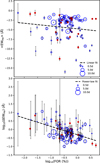 |
Fig. 11 FOR vs. Hα activity indicator. Upper panel: linear fit as ⟨EWHα⟩ = a [log10(FOR)] + b, where a = −0.72 ± 0.63 and b = −4.75 ± 0.42. Lower panel: power-law fit as ΔEWHα = k (FOR)α, where k = 0.485 ± 0.058 and α = −0.492 ± 0.076. The symbols have the same meaning as in Fig. 4. |
4.6 Starspot filling factor (fs)
It is well known that the observed brightness variation in the light curve arises from starspots in the stellar photosphere (Fang et al. 2016). Because of their unstable nature, these starspots can move across the stellar surface; their amplitudes fluctuate significantly within each rotation period. This variability might contribute to the fact that the observed radii of young low-mass active stars are larger than predicted by theories (Stauffer et al. 2007; Jackson et al. 2009).
Kumar et al. (2023) used the relation by (Jackson & Jeffries 2013) and calculated the starspot filling factor (fs), which gives the fractional area covered by starspots (Aspot/A⋆). In Figure 15 we show the correlation between fs and Teff. The fs of M dwarfs in our sample is spread over a wide range, indicating potential effects from other parameters on stellar spot coverage. More interestingly, fs decreases from cooler M dwarfs to hotter M dwarfs, with a plateau in the spot coverage at ~4% over the Teff interval from ~2900 to ~3600 K, indicating a saturation-like phase similar to chromospheric and coronal activities observed in fast-rotating stars. In Figure 16 we show the correlation between fs and flare activity. The weak positive trend (dashed black line) suggests that higher flare activity is associated with a larger coverage of active regions on M dwarfs. This is expected because strong magnetic activity is often associated with large starspot coverage on active M dwarfs (Yang et al. 2017; Medina et al. 2022).
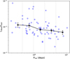 |
Fig. 12 Distribution of Lflare/Lbol with Prot for M dwarfs. The blue circles represent individual stars. The black squares represent the median values in five equally spaced bins (log scale). The error bars in the median values are discussed in Section 4.2. |
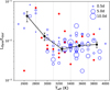 |
Fig. 13 Distribution of Teff with Lflare/Lbol. The black squares represent the median values in five equally spaced bins. The symbols have the same meaning as in Fig. 4. |
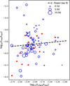 |
Fig. 14 Lflare/Lbol vs. LHα/Lbol. The dashed black line shows the power-law fitting as LHα/Lbol = k (Lflare/Lbol)α, where k=(1.83±0.63)×10−4 and α=0.053±0.072. The symbols have the same meaning as in Fig. 4. |
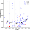 |
Fig. 15 Distribution of the derived fs with Teff. The black squares represent the median values within five equally spaced bins. The symbols have the same meaning as in Fig. 4. |
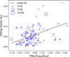 |
Fig. 16 Distribution of the derived fs with Lflare/Lbol. The dashed black line shows the linear fitting as |
![$\[f_{s}=a ~\log _{10}\left(\frac{L_{\text {flare}}}{L_{\text {bol}}}\right)+b\]$](/articles/aa/full_html/2025/12/aa54816-25/aa54816-25-eq10.png)
5 Conclusion
We used photometric data from TESS and spectroscopic data from the MFOSC-P spectrograph. We characterized the stellar activity through FOR, flare energies, starspot-filling factors, chromospheric activity indicators such as Hα emission, and their dependence on stellar mass, spectral type, and rotation period. For a convective M dwarf, the magnitude of the stellar activity is known to be linked to the magnetic properties and to the state of the star.
Our study demonstrated that the flaring in M dwarfs is linked to their spectral type, mass, and rotation. For early- to mid-type M dwarfs (M0–M4), we found that FOR exhibits a nearly flat distribution that starts to decline for later spectral types. This suggests that a transition in magnetic activity occurs near M4, possibly due to the transition to fully convective interiors. Rapid rotators (Prot < 1 day) exhibit significantly higher FOR, which supports the idea that strong magnetic dynamos in fast-rotating M dwarfs sustain frequent flaring activity.
The negative correlation between FOR and flare amplitude indicates that more frequently, flaring M dwarfs tend to produce less energetic flares. Our results agree with previous findings, which suggested that highly active stars dissipate magnetic energy through numerous low-energy flares rather than fewer high-energy events. Furthermore, our analysis of FFDs for different spectral types revealed that α systematically increases from M0 (α ~ 1.68) to M5 (α ~ 1.95). This trend suggests that flare frequency distributions become steeper for later-type M dwarfs, meaning that high-energy flares become even rarer.
Chromospheric activity, traced using the Hα EW and LHα/Lbol, shows that M dwarfs with stronger Hα activity tend to exhibit higher FOR. Our spectroscopic analysis revealed a 92% decrease in ΔEW for the studied stellar mass range, which may be attributed to fundamental changes in the magnetic field generation process as M dwarfs transition to fully convective interiors.
We also found that the fs decreases with increasing temperature and exhibits a saturation-like behavior in stars with Teff ~ 2900–3600 K. This suggests that strong magnetic activity in fast-rotating M dwarfs results in substantial spot coverage, which might affect their observed stellar radii and rotational evolution.
Our analysis also confirmed the strong correlation between LHα/Lbol and Lflare/Lbol, following a power-law relation. Even a small increase in chromospheric activity can lead to a significant rise in flare energy. This supports the idea that superflares in M dwarfs do not necessarily require an additional energy-generation mechanism. Instead, they might result naturally from enhanced magnetic activity.
Our study of flaring M dwarfs contributes to the broader understanding of stellar magnetic activity in these fast-rotating cool objects. High-cadence photometric and spectroscopic observations in the future are crucial to refine these relations further and extend our understanding of activity trends in slowly rotating M dwarfs (Prot > 10 days).
Data availability
Tables A.1, A.2 and B.1 are available at the CDS via https://cdsarc.cds.unistra.fr/viz-bin/cat/J/A+A/704/A154.
Acknowledgements
A.S.R. is thankful to the staff at the Mount Abu Observatory for their invaluable assistance during the observations. The MFOSC-P instrument is funded by the Department of Space, Government of India, through the Physical Research Laboratory. M.K.S. thanks the Director, PRL, for supporting the MFOSC-P development program. V.K. thanks the German Federal Department for Education and Research (Bundesministerium für Bildung und Forschung - BMBF) under grant agreement (Verbundforschung) number 05A23PK1 for partially supporting this research. L.L. gratefully acknowledges the Collaborative Research Centre 1601 funded by the Deutsche Forschungsgemeinschaft (DFG, German Research Foundation)—SFB 1601 [sub-project A3]— 500700252. J.G.F-T gratefully acknowledges the grant support provided by ANID Fondecyt Postdoc No. 3230001(Sponsoring researcher), and from the Joint Committee ESO-Government of Chile under the agreement 2023 ORP 062/2023. The data from the Transiting Exoplanet Survey Satellite (TESS) was acquired using the tessilator software package. This research has made use of the Exoplanet Follow-up Observation Program (ExoFOP; DOI: 10.26134/ExoFOP5) website, which is operated by the California Institute of Technology, under contract with the National Aeronautics and Space Administration under the Exoplanet Exploration Program.
References
- Amado, P. J., Bauer, F. F., Rodríguez López, C., et al. 2021, A&A, 650, A188 [NASA ADS] [CrossRef] [EDP Sciences] [Google Scholar]
- Anders, F., Khalatyan, A., Chiappini, C., et al. 2019, A&A, 628, A94 [NASA ADS] [CrossRef] [EDP Sciences] [Google Scholar]
- Anglada-Escudé, G., Amado, P. J., Barnes, J., et al. 2016, Nature, 536, 437 [Google Scholar]
- Astudillo-Defru, N., Forveille, T., Bonfils, X., et al. 2017, A&A, 602, A88 [NASA ADS] [CrossRef] [EDP Sciences] [Google Scholar]
- Benedict, G. F., Henry, T. J., Franz, O. G., et al. 2016, AJ, 152, 141 [Google Scholar]
- Benz, A. O., & Güdel, M. 2010, ARA&A, 48, 241 [NASA ADS] [CrossRef] [Google Scholar]
- Binks, A. S., & Günther, H. M. 2024, MNRAS, 533, 2162 [Google Scholar]
- Bouchy, F., Doyon, R., Pepe, F., et al. 2025, A&A, 700, A10 [NASA ADS] [CrossRef] [EDP Sciences] [Google Scholar]
- Caldwell, D. A., Tenenbaum, P., Twicken, J. D., et al. 2020, Res. Notes Am. Astron. Soc., 4, 201 [Google Scholar]
- Candelaresi, S., Hillier, A., Maehara, H., Brandenburg, A., & Shibata, K. 2014, ApJ, 792, 67 [NASA ADS] [CrossRef] [Google Scholar]
- Cao, D.-t., & Gu, S.-h. 2014, AJ, 147, 38 [NASA ADS] [CrossRef] [Google Scholar]
- Cersullo, F., Wildi, F., Chazelas, B., & Pepe, F. 2017, A&A, 601, A102 [NASA ADS] [CrossRef] [EDP Sciences] [Google Scholar]
- Chang, S.-W., Byun, Y.-I., & Hartman, J. D. 2015, ApJ, 814, 35 [NASA ADS] [CrossRef] [Google Scholar]
- Chang, H. Y., Song, Y. H., Luo, A. L., et al. 2017, ApJ, 834, 92 [NASA ADS] [CrossRef] [Google Scholar]
- Cincunegui, C., Díaz, R. F., & Mauas, P. J. D. 2007, A&A, 469, 309 [NASA ADS] [CrossRef] [EDP Sciences] [Google Scholar]
- Cosentino, R., Lovis, C., Pepe, F., et al. 2012, Proc. SPIE, 8446, 84461V [Google Scholar]
- Crowley, J., Wheatland, M. S., & Yang, K. 2024, MNRAS, 530, 457 [Google Scholar]
- Davenport, J. R. A. 2016, ApJ, 829, 23 [Google Scholar]
- Davenport, J. R. A., Hawley, S. L., Hebb, L., et al. 2014, ApJ, 797, 122 [Google Scholar]
- Díaz, R. F., González, J. F., Cincunegui, C., & Mauas, P. J. D. 2007, A&A, 474, 345 [NASA ADS] [CrossRef] [EDP Sciences] [Google Scholar]
- Donati, J. F., Cristofari, P. I., Finociety, B., et al. 2023, MNRAS, 525, 455 [NASA ADS] [CrossRef] [Google Scholar]
- Donati, J. F., Cristofari, P. I., Lehmann, L. T., et al. 2024, MNRAS, 531, 3256 [Google Scholar]
- Doyle, L., Ramsay, G., Doyle, J. G., Wu, K., & Scullion, E. 2018, MNRAS, 480, 2153 [Google Scholar]
- Doyle, L., Ramsay, G., Doyle, J. G., & Wu, K. 2019, MNRAS, 489, 437 [Google Scholar]
- Fang, X.-S., Zhao, G., Zhao, J.-K., Chen, Y.-Q., & Bharat Kumar, Y. 2016, MNRAS, 463, 2494 [NASA ADS] [CrossRef] [Google Scholar]
- Feinstein, A. D., Montet, B. T., Ansdell, M., et al. 2020, AJ, 160, 219 [Google Scholar]
- Fontenla, J. M., Linsky, J. L., Garrison, J., et al. 2016, ApJ, 830, 154 [NASA ADS] [CrossRef] [Google Scholar]
- Gao, Q., Xin, Y., Liu, J.-F., Zhang, X.-B., & Gao, S. 2016, ApJS, 224, 37 [NASA ADS] [CrossRef] [Google Scholar]
- Gomes da Silva, J., Santos, N. C., Bonfils, X., et al. 2011, A&A, 534, A30 [NASA ADS] [CrossRef] [EDP Sciences] [Google Scholar]
- Green, P. J., & Margon, B. 1994, ApJ, 423, 723 [Google Scholar]
- Günther, M. N., Zhan, Z., Seager, S., et al. 2020, AJ, 159, 60 [Google Scholar]
- Hawley, S. L., Davenport, J. R. A., Kowalski, A. F., et al. 2014, ApJ, 797, 121 [Google Scholar]
- Henry, T. J. 1998, ASP Conf. Ser., 134, 28 [Google Scholar]
- Hilton, E. J., West, A. A., Hawley, S. L., & Kowalski, A. F. 2010, AJ, 140, 1402 [Google Scholar]
- Howell, S. B., Sobeck, C., Haas, M., et al. 2014, PASP, 126, 398 [Google Scholar]
- Ilin, E., Schmidt, S. J., Poppenhäger, K., et al. 2021, A&A, 645, A42 [NASA ADS] [CrossRef] [EDP Sciences] [Google Scholar]
- Jackman, J. A. G., Wheatley, P. J., Acton, J. S., et al. 2021, MNRAS, 504, 3246 [NASA ADS] [CrossRef] [Google Scholar]
- Jackson, R. J., & Jeffries, R. D. 2013, MNRAS, 431, 1883 [Google Scholar]
- Jackson, R. J., Jeffries, R. D., & Maxted, P. F. L. 2009, MNRAS, 399, L89 [NASA ADS] [CrossRef] [Google Scholar]
- Jenkins, J. M., Twicken, J. D., McCauliff, S., et al. 2016, SPIE Conf. Ser., 9913, 99133E [Google Scholar]
- Kaeufl, H.-U., Ballester, P., Biereichel, P., et al. 2004, Proc. SPIE, 5492, 1218 [CrossRef] [Google Scholar]
- Klein, B., Zicher, N., Kavanagh, R. D., et al. 2022, MNRAS, 512, 5067 [NASA ADS] [CrossRef] [Google Scholar]
- Kossakowski, D., Kürster, M., Trifonov, T., et al. 2023, A&A, 670, A84 [NASA ADS] [CrossRef] [EDP Sciences] [Google Scholar]
- Kretzschmar, M. 2011, A&A, 530, A84 [NASA ADS] [CrossRef] [EDP Sciences] [Google Scholar]
- Kumar, V., Rajpurohit, A. S., Srivastava, M. K., Fernández-Trincado, J. G., & Queiroz, A. B. A. 2023, MNRAS, 524, 6085 [Google Scholar]
- Leenaarts, J., Carlsson, M., & Rouppe van der Voort, L. 2012, ApJ, 749, 136 [NASA ADS] [CrossRef] [Google Scholar]
- Lin, C. L., Ip, W. H., Hou, W. C., Huang, L. C., & Chang, H. Y. 2019, ApJ, 873, 97 [NASA ADS] [CrossRef] [Google Scholar]
- Luque, R., Fulton, B. J., Kunimoto, M., et al. 2022, A&A, 664, A199 [NASA ADS] [CrossRef] [EDP Sciences] [Google Scholar]
- Maehara, H., Shibayama, T., Notsu, S., et al. 2012, Nature, 485, 478 [NASA ADS] [Google Scholar]
- Magaudda, E., Stelzer, B., Covey, K. R., et al. 2020, A&A, 638, A20 [NASA ADS] [CrossRef] [EDP Sciences] [Google Scholar]
- Mahadevan, S., Ramsey, L., Bender, C., et al. 2012, Proc. SPIE, 8446, 84461S [Google Scholar]
- Mann, A. W., Feiden, G. A., Gaidos, E., Boyajian, T., & von Braun, K. 2015, ApJ, 804, 64 [Google Scholar]
- Mauas, P. J. D., & Falchi, A. 1994, A&A, 281, 129 [NASA ADS] [Google Scholar]
- Mayor, M., Pepe, F., Queloz, D., et al. 2003, The Messenger, 114, 20 [NASA ADS] [Google Scholar]
- Mazeh, T., Perets, H. B., McQuillan, A., & Goldstein, E. S. 2015, ApJ, 801, 3 [Google Scholar]
- Medina, A. A., Charbonneau, D., Winters, J. G., Irwin, J., & Mink, J. 2022, ApJ, 928, 185 [NASA ADS] [CrossRef] [Google Scholar]
- Meng, G., Zhang, L.-Y., Su, T., et al. 2023, Res. Astron. Astrophys., 23, 055001 [CrossRef] [Google Scholar]
- Newton, E. R., Irwin, J., Charbonneau, D., et al. 2017, ApJ, 834, 85 [Google Scholar]
- Notsu, Y., Shibayama, T., Maehara, H., et al. 2013, ApJ, 771, 127 [NASA ADS] [CrossRef] [Google Scholar]
- Noyes, R. W., Hartmann, L. W., Baliunas, S. L., Duncan, D. K., & Vaughan, A. H. 1984, ApJ, 279, 763 [Google Scholar]
- Parnell, C. E., & Jupp, P. E. 2000, ApJ, 529, 554 [Google Scholar]
- Pettersen, B. R., & Hawley, S. L. 1989, A&A, 217, 187 [NASA ADS] [Google Scholar]
- Queiroz, A. B. A., Anders, F., Santiago, B. X., et al. 2018, MNRAS, 476, 2556 [Google Scholar]
- Quirrenbach, A., Amado, P. J., Caballero, J. A., et al. 2014, Proc. SPIE, 9147, 91471F [Google Scholar]
- Raetz, S., Stelzer, B., Damasso, M., & Scholz, A. 2020, A&A, 637, A22 [NASA ADS] [CrossRef] [EDP Sciences] [Google Scholar]
- Rajpurohit, A. S., Kumar, V., Srivastava, M. K., et al. 2020, MNRAS, 492, 5844 [Google Scholar]
- Ramsay, G., Doyle, J. G., Hakala, P., et al. 2013, MNRAS, 434, 2451 [Google Scholar]
- Reid, I. N., Hawley, S. L., & Gizis, J. E. 1995, AJ, 110, 1838 [Google Scholar]
- Reiners, A., Joshi, N., & Goldman, B. 2012, AJ, 143, 93 [Google Scholar]
- Reinhold, T., Cameron, R. H., & Gizon, L. 2017, A&A, 603, A52 [NASA ADS] [CrossRef] [EDP Sciences] [Google Scholar]
- Reylé, C., Jardine, K., Fouqué, P., et al. 2021, A&A, 650, A201 [Google Scholar]
- Ricker, G. R., Winn, J. N., Vanderspek, R., et al. 2015, J. Astron. Telesc. Instrum. Syst., 1, 014003 [Google Scholar]
- Robertson, P., Endl, M., Cochran, W. D., & Dodson-Robinson, S. E. 2013, ApJ, 764, 3 [Google Scholar]
- Savitzky, A., & Golay, M. J. E. 1964, Anal. Chem., 36, 1627 [Google Scholar]
- Shibayama, T., Maehara, H., Notsu, S., et al. 2013, ApJS, 209, 5 [Google Scholar]
- Srivastava, M. K., Jangra, M., Dixit, V., et al. 2018, SPIE Conf. Ser., 10702, 107024I [Google Scholar]
- Srivastava, M. K., Kumar, V., Dixit, V., et al. 2021, Exp. Astron. [arXiv:2104.00314] [Google Scholar]
- Stassun, K. G., Oelkers, R. J., Pepper, J., et al. 2018, AJ, 156, 102 [Google Scholar]
- Stauffer, J. R., Hartmann, L. W., Fazio, G. G., et al. 2007, ApJS, 172, 663 [NASA ADS] [CrossRef] [Google Scholar]
- Stelzer, B., Damasso, M., Scholz, A., & Matt, S. P. 2016, MNRAS, 463, 1844 [NASA ADS] [CrossRef] [Google Scholar]
- Stelzer, B., Bogner, M., Magaudda, E., & Raetz, S. 2022, A&A, 665, A30 [NASA ADS] [CrossRef] [EDP Sciences] [Google Scholar]
- Tilley, M. A., Segura, A., Meadows, V., Hawley, S., & Davenport, J. 2019, Astrobiology, 19, 64 [Google Scholar]
- Walkowicz, L. M., Basri, G., Batalha, N., et al. 2011, AJ, 141, 50 [NASA ADS] [CrossRef] [Google Scholar]
- West, A. A., Hawley, S. L., Walkowicz, L. M., et al. 2004, AJ, 128, 426 [NASA ADS] [CrossRef] [Google Scholar]
- West, A. A., Weisenburger, K. L., Irwin, J., et al. 2015, ApJ, 812, 3 [NASA ADS] [CrossRef] [Google Scholar]
- Wright, N. J., Drake, J. J., Mamajek, E. E., & Henry, G. W. 2011, ApJ, 743, 48 [Google Scholar]
- Yang, H., Liu, J., Gao, Q., et al. 2017, ApJ, 849, 36 [NASA ADS] [CrossRef] [Google Scholar]
- Yang, Z., Zhang, L., Meng, G., et al. 2023, A&A, 669, A15 [NASA ADS] [CrossRef] [EDP Sciences] [Google Scholar]
- Zhang, L.-Y., Long, L., Shi, J., et al. 2020, MNRAS, 495, 1252 [NASA ADS] [CrossRef] [Google Scholar]
All Tables
All Figures
|
Fig. 1 Distance distribution (top panel) of stars in our sample, binned at 5 pc intervals, and the TESS magnitude distribution (bottom panel) of the same sample. |
| In the text | |
|
Fig. 2 Top panel: TESS light curve of PM J16170+5516 (M2.0) from Sector-25, 2020 (SPOC) with Prot 1.975 days. The black line shows the light curve with a cadence of 2 min, and the red line represents the Savitzky–Golay filtered and smoothed curve. Bottom panels: zoomed views of the detrended flux highlighting multiple flare events of different magnitudes. |
| In the text | |
|
Fig. 3 Temporal variation in the Hα line profiles for PM J12142+0037 (M4.0) since the beginning of the first exposure. The dashed lines indicate the pseudo-continuum regions. The equivalent widths are marked to the left of each emission line, and elapsed times since the initial exposure are shown on the right. |
| In the text | |
|
Fig. 4 Variability and activity indicators as a function of stellar mass. Top panel: Distribution of ΔEW = max(EW) – min(EW) for Hα emission. The dashed black line shows a linear fit, ΔEWHα = a(M*) + b, with a = 7.71 ± 1.55, b = −7.38 ± 0.64. Bottom panel: Median values of log10(LHα/Lbol) for Hα emission as a function of stellar mass. The black squares mark the medians in seven equally spaced bins with scatter quantified using the median absolute deviation. The blue circles are scaled by Prot, and larger circles correspond to longer Prot. The filled red circles indicate stars without a measured rotation period. The vertical gray lines show the bin sizes. |
| In the text | |
|
Fig. 5 Distribution of flare durations for M dwarfs (in minutes) shown for spectral subtypes M0–M6.5. |
| In the text | |
|
Fig. 6 Flare energy–duration relation for M dwarfs. The dashed red line shows the power-law fit (see Section 3.4). |
| In the text | |
|
Fig. 7 Cumulative flare frequency distribution for M dwarfs plotted as a function of flare energy for the spectral types. The dashed red line shows the power-law fit (see Section 3.4). For the M6–M6.5 sample, no fit is shown because there were too few flares. |
| In the text | |
|
Fig. 8 FOR vs. Teff for M dwarfs. The black squares show the median values in five equally spaced bins. The symbols have the same meaning as in Fig. 4. |
| In the text | |
|
Fig. 9 FOR as a function of Prot. The blue circles represent individual stars. The black square marks the median values in five equally spaced bins on a log scale. The error bars on the medians are discussed in Section 4.2. |
| In the text | |
|
Fig. 10 Flare amplitude vs. FOR. The dashed line shows the best-fit power law, FOR = k (flare amplitude)α, where k = 0.032 ± 0.01 and α = −0.8 ± 0.09. The symbols have the same meaning as in Fig. 4. |
| In the text | |
|
Fig. 11 FOR vs. Hα activity indicator. Upper panel: linear fit as ⟨EWHα⟩ = a [log10(FOR)] + b, where a = −0.72 ± 0.63 and b = −4.75 ± 0.42. Lower panel: power-law fit as ΔEWHα = k (FOR)α, where k = 0.485 ± 0.058 and α = −0.492 ± 0.076. The symbols have the same meaning as in Fig. 4. |
| In the text | |
|
Fig. 12 Distribution of Lflare/Lbol with Prot for M dwarfs. The blue circles represent individual stars. The black squares represent the median values in five equally spaced bins (log scale). The error bars in the median values are discussed in Section 4.2. |
| In the text | |
|
Fig. 13 Distribution of Teff with Lflare/Lbol. The black squares represent the median values in five equally spaced bins. The symbols have the same meaning as in Fig. 4. |
| In the text | |
|
Fig. 14 Lflare/Lbol vs. LHα/Lbol. The dashed black line shows the power-law fitting as LHα/Lbol = k (Lflare/Lbol)α, where k=(1.83±0.63)×10−4 and α=0.053±0.072. The symbols have the same meaning as in Fig. 4. |
| In the text | |
|
Fig. 15 Distribution of the derived fs with Teff. The black squares represent the median values within five equally spaced bins. The symbols have the same meaning as in Fig. 4. |
| In the text | |
|
Fig. 16 Distribution of the derived fs with Lflare/Lbol. The dashed black line shows the linear fitting as |
| In the text | |
Current usage metrics show cumulative count of Article Views (full-text article views including HTML views, PDF and ePub downloads, according to the available data) and Abstracts Views on Vision4Press platform.
Data correspond to usage on the plateform after 2015. The current usage metrics is available 48-96 hours after online publication and is updated daily on week days.
Initial download of the metrics may take a while.