| Issue |
A&A
Volume 704, December 2025
|
|
|---|---|---|
| Article Number | A219 | |
| Number of page(s) | 29 | |
| Section | Stellar structure and evolution | |
| DOI | https://doi.org/10.1051/0004-6361/202554874 | |
| Published online | 12 December 2025 | |
Populations of evolved massive binary stars in the Small Magellanic Cloud
II. Predictions from rapid binary evolution
1
Argelander-Institut für Astronomie, Universität Bonn, Auf dem Hügel 71, 53121 Bonn, Germany
2
Max-Planck-Institut für Radioastronomie, Auf dem Hügel 69, 53121 Bonn, Germany
3
Instituto de Astrofísica de Canarias, 38200 La Laguna, Tenerife, Spain
4
Departamento de Astrofísica, Universidad de La Laguna, 38205 La Laguna, Tenerife, Spain
5
Département d’Astronomie, Université de Genève, Chemin Pegasi 51, CH-1290 Versoix, Switzerland
6
Gravitational Wave Science Center (GWSC), Université de Genève, 24 Quai E. Ansermet, CH-1211 Geneva, Switzerland
7
Institute of Astrophysics, Foundation for Research & Technology Hellas (FORTH), GR-70013 Heraklion, Greece
8
Max-Planck-Institut für Extraterrestrische Physik, Gießenbachstraße 1, 85748 Garching, Germany
9
Tel Aviv University, The School of Physics and Astronomy, Tel Aviv 6997801, Israel
10
Department of Materials and Production, Aalborg University, Fibigerstræde 16, 9220 Aalborg, Denmark
11
School of Astronomy and Space Science, Nanjing University, Nanjing 210023, People’s Republic of China
12
Key Laboratory of Modern Astronomy and Astrophysics, Nanjing University, Ministry of Education, Nanjing 210023, People’s Republic of China
13
Max-Planck-Institut für Astrophysik, Karl-Schwarzschild-Straße 1, 85748 Garching, Germany
★ Corresponding authors: This email address is being protected from spambots. You need JavaScript enabled to view it.
; This email address is being protected from spambots. You need JavaScript enabled to view it.
Received:
30
March
2025
Accepted:
14
August
2025
Abstract
Context. Massive star evolution plays a crucial role in astrophysics; however, its study is subject to large uncertainties. This problem becomes more severe by the majority of massive stars being born in close binary systems, whose evolution is affected by interactions among their components.
Aims. We want to constrain major uncertainties in massive binary star evolution, particularly with respect to the efficiency and the stability of the first mass-transfer phase.
Methods. We used the rapid population synthesis code COMBINE to generate synthetic populations of post-interaction binaries, assuming constant mass-transfer efficiency. We employed a new merger criterion that adjusts self-consistently to any prescribed mass-transfer efficiency. We tailored our synthetic populations to be comparable to the expected binary populations in the Small Magellanic Cloud (SMC).
Results. We find that the observed populations of evolved massive binaries cannot be reproduced with a single mass-transfer efficiency. Instead, a rather high efficiency (≳50%) is needed to reproduce the number of Be stars and Be/X-ray (BeXB) binaries in the SMC, while a low efficiency (∼10%) leads to a better agreement with the observed number of Wolf-Rayet (WR) stars. We constructed a corresponding mass-dependent mass-transfer efficiency recipe to produce our fiducial synthetic SMC post-interaction binary population. It reproduces the observed number and properties of the BeXBs and WR binaries rather well; furthermore, it is not in stark disagreement with the observed OBe star population. It predicts around 170 massive stars with neutron star companion, of which 140 are Be stars, and about 170 systems disrupted by the supernova, of which 150 are Be stars. Overall, 20% of all post-interaction systems contain a helium star. It also predicts two large, as-yet-unobserved populations of OB + BH binaries: about 100 OB + BH systems with rather small orbital periods (≲20 d) and around 40 longer period OBe + BH systems.
Conclusions. Continued searches for massive binary systems will strongly advance our understanding of their evolution.
Key words: stars: black holes / stars: emission-line, Be / stars: massive / stars: neutron / Magellanic Clouds / X-rays: binaries
© The Authors 2025
 Open Access article, published by EDP Sciences, under the terms of the Creative Commons Attribution License (https://creativecommons.org/licenses/by/4.0), which permits unrestricted use, distribution, and reproduction in any medium, provided the original work is properly cited.
This article is published in open access under the Subscribe to Open model. This email address is being protected from spambots. You need JavaScript enabled to view it. to support open access publication.
1. Introduction
Massive stars are powerful cosmic engines. They produce spectacular events such as supernovae (SNe) and gamma-ray bursts, drive the chemical evolution of galaxies (Timmes et al. 1995) and shape their interstellar medium (Hopkins et al. 2014). Massive stars are preferentially born in close binary systems (Sana et al. 2012), which produce X-ray binaries and gravitational wave mergers (Tauris & van den Heuvel 2006, 2023). However, our understanding of their evolution is far from complete (Langer 2012, 2024).
The different types of massive binaries can be ordered in a simplified evolution scheme (e.g. Tauris & van den Heuvel 2006) from zero-age main-sequence (ZAMS) binaries up to compact object mergers (Fig. 1). However, the vast majority of massive binary stars will exit the evolutionary path, either by breaking up as a consequence of core collapse (Tauris & Takens 1998) or by merging into a single object due to the interaction between the two stellar components (Podsiadlowski et al. 1992; Langer 2012; de Mink et al. 2014). A critical step in this evolutionary scheme is the Roche-lobe overflow (RLO), where matter is transferred from one star (donor) to the other (accretor) (Kippenhahn & Weigert 1967). In the first RLO, it is usually the heavier star that is the donor as it burns its fuel faster and expands first. This process can either take place during its main-sequence phase (Case A) or during shell burning (Case B; Kippenhahn & Weigert 1967). The physics of the RLO is not well understood, especially with respect to the conditions that determine whether we are dealing with a case of donor stripping or a merger (Ivanova et al. 2013), what fraction of material lost by the donor is deposited on the accretor (de Mink et al. 2007), and how much angular momentum the ejected material removes from the system (Marchant & Bodensteiner 2024).
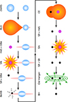 |
Fig. 1. Schematic evolutionary path from ZAMS to gravitational wave merger, adapted from Kruckow et al. (2018). We focus on the BH + OBe phase. |
Stable mass transfer is expected to lead to an almost complete removal of the hydrogen-rich envelope of the donor. While this stripped star may retain a thin hydrogen layer (Gilkis et al. 2019; Laplace et al. 2020) or may only partially strip (Ercolino et al. 2024), it is commonly referred to as a helium star (HeS). The accretor receives mass, which may rejuvenate the star (Braun & Langer 1995), and gains spin angular momentum. Packet (1981) showed that only a small amount of accreted material is enough to bring the accretor to rotate close to critical rotation.
Rotating near critical rotation, such a star expels matter from its surface, forming a decretion disk around its equator. This disk causes broad emission lines to appear in the spectrum. These lines, along with the rotationally broadened absorption lines of the star serve as an explanation for the Be star phenomenon (Porter & Rivinius 2003; Rivinius et al. 2013). It is, however, possible that either the mass loss (and thus angular momentum loss) or tidal forces brake stellar rotation; alternatively, strong stellar winds could remove the disk so that the OBe star becomes a usual OB star again. On the other hand, it could be the case that the HeS expands so much that it initiates a second mass transfer (Case BB/BC; Tauris et al. 2015). The HeS terminates its life shortly after and becomes a stellar remnant (SR), namely a white dwarf (WD), neutron star (NS), or a black hole (BH). The following phase (OB + SR) is the focus of this work, as it is the second best observable one, since it features a long-living main-sequence star and an inert SR.
This formation channel of OBe stars by binary interaction is supported by the fact that no OBe stars with main-sequence companions have been observed (Bodensteiner et al. 2020) and, on the other hand, OBe stars with hot subdwarf (sdOB; the observational counterpart to light HeSs; Wang et al. 2021), WD (Zhu et al. 2023), and NS (Coe & Kirk 2015) companions are well known. However, only a few Be + sdOB and Be + WD systems have been discovered since the light and faint companion is hard to detect (Coe et al. 2020; Kennea et al. 2021; Gaudin et al. 2024; Marino et al. 2025). However, they can be very X-ray bright (Eddington luminosity) when they show nova-like outbursts. Several of these systems have been discovered recently (Marino et al. 2025, and references therein). Be + NS systems often appear as BeXBs as the NS accretes material from the disk and releases X-ray emission. Another proposed formation process of OBe stars is single-star evolution, which was recently studied by Ekström et al. (2008) and Hastings et al. (2020).
The success of this picture gives rise to questions around configurations that have not yet been observed. In particular, as many massive stars with NS companions are known, we would assume that OBe star systems with BH companions exist as well. Today, only one system of that kind has been proposed (MWC 656; Casares et al. 2014), but its nature was recently disputed by two independent studies (Rivinius et al. 2024; Janssens et al. 2023). On the other hand, three super-giant/X-ray binaries with BHs (Cyg X-1, LMC X-1, and M33 X-7) are well observed (Orosz et al. 2007, 2009, 2011; Miller-Jones et al. 2021; Ramachandran et al. 2022) and even one source with an X-ray quiet BH is known (VFTS 243, Shenar et al. 2022a). Therefore, an objective of this study is to answer whether it is possible to form OBe + BH systems and to predict their properties. After the OBe + SR phase, the system can evolve through a common envelope ejection to a binary SR, which may undergo a gravitational wave merger (Fig. 1). Thus, the OB + SR phase is an important intermediate step in understanding binary stellar evolution as a whole.
In this study, we focus on stars in the Small Magellanic Cloud (SMC). As a low-metallicity satellite galaxy of the Milky Way, it is a distinctive environment. Its metallicity of about one-fifth of the solar value (Venn 1999; Korn et al. 2000; Hunter et al. 2008) corresponds to the average metallicity of a redshift of about 3 (Kewley & Kobulnicky 2007). Low metallicities are interesting, as the aforementioned events (SNe, gamma-ray bursts, and gravitational waves) originate predominately in low metallicity environments (Abbott et al. 2019, 2023); thus, they have been recently studied extensively (e.g. Ge et al. 2023, and references therein). Being located at a distance of about 60 kpc, observing individual stars is still possible, as currently carried out by the ‘Binarity at LOw Metallicity’ (BLOeM) campaign (Shenar et al. 2024), which should yield robust constraints on many of the predictions presented in this work. Another advantage of SMC is the weaker stellar winds caused by low metallicity (Abbott 1982; Kudritzki et al. 1987; Mokiem et al. 2007). Lower winds imply a lower loss of angular momentum and, thus, we expect OBe stars to be more numerous and exhibit higher masses as well as, hence, a higher success rate in finding OBe + BH systems.
This study is closely related to Xu et al. (2025, hereafter Paper I), who investigated the same types of objects using detailed stellar models, whereas we used rapid binary evolution, which requires significantly fewer computational resources. This gives us the opportunity to investigate an alternative approach to treating the RLO phase that involves conducting a comprehensive study of the unconstrained parameters. Our work is structured as follows. Sect. 2 describes our methods to simulate systems consisting of a hydrogen-burning star with an SR. In Sect. 3, we describe how the outcome of binary evolution code depends on the initial parameters of the binary. In Sect. 4, we use different physical assumptions to generate artificial populations and compare them to observational characteristics to determine a fiducial set of assumptions. The population based on these assumptions is analysed in detail in Sect. 5. In Sect. 6, we compare our results to observations and previous work. A summary of our conclusions is given in Sect. 7.
2. Method
We investigated the OB + SR population of the SMC with the Monte Carlo based rapid binary population synthesis code COMBINE, which was first introduced by Kruckow et al. (2018). In this section, we describe how this code operates and how we adjusted it for this study.
2.1. The rapid binary population synthesis code COMBINE
Evolving both binary components simultaneously, COMBINE is based on tabulated detailed single-star models, in contrast to other binary population synthesis codes, which treat stellar evolution using fitting formulae. This allows for a fast exchange and modular use of the underlying stellar models. Compared to detailed codes such as MESA (Paxton et al. 2019, and references therein), COMBINE is much faster and enables the user to generate large model populations of different underlying binary physics in a small amount of time. Also, in contrast to MESA, it follows a system’s evolution through a SN event and it is able to treat a common envelope phase; also, in contrast to other rapid binary population synthesis codes, it uses envelope binding energies calculated self consistently from stellar models (Kruckow et al. 2016), rather than constant values of the envelope’s binding energy or mixing results of different 1D stellar evolution codes.
The dense grid of detailed stellar models is currently available for Milky Way, Large Magellanic Cloud (LMC), SMC, and I Zwicky 18 metallicity, featuring both hydrogen-rich and HeS models. The models were calculated with BEC (Yoon et al. 2010, and references therein) using the same stellar physics as Brott et al. (2011) with initial masses from 0.5 to 100 M⊙. For the application in COMBINE, the following quantities were extracted and tabulated: total stellar mass, age, photospheric radius, core mass (see Sect. 2.2 for the updated definition), luminosity, effective temperature, two versions of the λ-parameter describing the binding energy of the envelope, and (new to this version of COMBINE, see Sect. 2.2) the carbon core mass and the moment of inertia factor. For hydrogen-rich models, the time of central hydrogen exhaustion is saved, too. Using initial mass and age as independent quantities, the current values of the remaining eight dependent quantities are interpolated linearly. The same HeS tracks are used for all metallicities, but their masses were rescaled by the wind mass loss rate, according to Hainich et al. (2015). While we are aware that detailed stellar models predict a small hydrogen layer to remain on the HeS and that the size of this layer has a large impact on the stellar radius (Laplace et al. 2020), we neglected it for simplicity.
To initialise a binary star model, COMBINE draws the initial primary mass M1 from an initial mass function (IMF). We used a Kroupa-like function, expressed as
 (1)
(1)
with a high mass slope of α = 2.3 (Salpeter 1955; Massey et al. 1995) within the range of 3–100 M⊙. The lower limit ensures that we consider all relevant stars to meaningfully compare the companions of NS to stars of similar mass and the upper limit is the mass of the most massive stellar model we have. The mass of the secondary is derived from a mass ratio distribution,
 (2)
(2)
and the initial separation from an orbital period distribution,
 (3)
(3)
To model the binary star population in the SMC, we relied on four sets of observationally inferred values of κ and π: Sana et al. (2012), based on Galactic O-type stars (κ = −0.1, π = −0.55); Sana et al. (2013), based on LMC O-type stars (κ = −1.0, π = −0.45); Dunstall et al. (2015), based on LMC early B-type stars (κ = −2.8, π = 0.0); and flat distributions, which were observed by Kobulnicky et al. (2014) in the Cygnus OB2 association (as well as Almeida et al. (2017, π = −0.1)) and Shenar et al. (2022b, with κ consistent with 0) (but we treated this mostly as an academic example). We note that these distributions might not be independent (Moe & Di Stefano 2017). While the lower orbital period limit is given naturally by RLO at ZAMS, we need to be careful about the upper limit. We chose to only consider orbital periods up to 103.5 d ≈ 3162 d, as this is the range considered by Sana et al. (2012), Sana et al. (2013), and Dunstall et al. (2015). As they noted that 50–70% of massive stars have orbital periods below that value and this upper limit coincides roughly with the maximum orbital period for RLO (see Sect. 3), the remaining fraction of stars is either single or in wide non-interacting binaries, rendering them effectively single for our purposes. We assumed a binary fraction of 100% and circular initial orbits, as tidal effects will circularise the orbit before the onset of RLO (Zahn 1977). As we implemented stellar rotation (see Sect. 2.3), it is also possible to choose the initial rotation of the models. We assumed no rotation, a bimodal distribution as in Dufton et al. (2013), synchronised (as in Langer et al. 2020), and a flat equatorial rotation distribution between zero and a user-determined value. We restricted the present study to initially synchronised stars, as tidal interaction predicts this to be archived during evolution towards RLO (Zahn 1977). We used the same stellar models for all rotation rates, which is justified for stars not too close to critical rotation (Brott et al. 2011).
After a system is initialised, it is evolved by COMBINE until only SRs remain. In practice, this means the code determines the time until the radius of one model becomes larger than the Roche radius according to the formula of Eggleton (1983), which marks the onset of an RLO or the end of the stellar evolution. For the intermediate time, the orbital period is adjusted to account for mass loss and the rotational velocity evolves as described in Sect. 2.3.
If one of the two stars is destined to overfill its Roche lobe, COMBINE evaluates whether the donor is stripped by stable mass transfer, a common envelope ejection occurs or the two stars merge. The criteria for that are discussed in Sect. 2.2. In case of stable mass transfer, COMBINE employs the analytical descriptions of Soberman et al. (1997) to describe the change in the orbital period. For this study, we assume that all ejected mass carries the same specific orbital angular momentum as the accretor. We assumed that the mass-transfer efficiency is constant throughout the RLO and treated it as a free parameter, whose value we chose to vary in this study. After the end of the mass transfer, COMBINE searches the stellar model grid for a new model for the accretor with matching core mass and total mass. Since the envelope mass increased, the new model appeared to be younger compared to the old model (rejuvenation). The donor was assumed to become a HeS and a matching model was determined from the HeS model grid. In case of a Case BB/BC RLO, when the donor is already a HeS, we assume an instant SN after the RLO. The duration of a Case B mass transfer was assumed to be of the order of a thermal timescale of the donor. For the duration of the Case A mass transfer and the donor mass thereafter see Sect. 2.2. All unstable RLOs were checked to determine whether a common envelope ejection is possible. We assumed, however, that all unstable RLOs lead to a merger (described in Sect. 2.2), as common envelope ejection is expected to take a very small fraction of the population considered in this study.
When the end of stellar evolution is reached, an SR is formed. Depending on the structure of the final stellar model, this is a WD, NS, or BH. If the helium core mass exceeds 6.6 M⊙, we assume a BH is formed (Sukhbold et al. 2018). The complete carbon core and 80% of the helium layer above it collapse into the BH, and we reduced that mass by 20% to account for the release of gravitational energy (Kruckow et al. 2018, and references therein). If the mass of the carbon core is above 1.435 M⊙, a NS is formed by a core collapse SN (CCSN); if it is between 1.37 M⊙ and 1.435 M⊙, we assume an electron capture SN (ECSN) as calculated by Tauris et al. (2015). The NS masses are around 1.3 M⊙ with the detailed formulae given in Kruckow et al. (2018). If the carbon core is lighter than 1.37 M⊙, a WD is formed, which inherits the progenitor’s carbon core mass as its total mass.
From the velocity distribution of young pulsars (Hobbs et al. 2005; Verbunt et al. 2017) it is known that a SN imposes a natal kick on the NSs. For ECSNe, our standard assumption is a uniformly distributed kick between 0 and 50 km/s (Podsiadlowski et al. 2004; Dessart et al. 2006; Kitaura et al. 2006). For the CCSN, we used a Maxwell-Boltzmann distribution for the kick velocity, w,
 (4)
(4)
with a 3D root-mean-square velocity (wrms) of  for H-rich progenitors (Hobbs et al. 2005),
  for HeS (Tauris & Bailes 1996; Tauris et al. 2017; Coleiro & Chaty 2013), and
  for SNe after Case BB/BC (Kruckow et al. 2018). Following Tauris et al. (2017) and Kruckow et al. (2018), we assumed that 20% of the systems with stripped stars receive a kick of
  . We varied these assumptions by running one scenario without SN kicks and one with only 3D root-mean-square velocities of
  . We refer to these scenarios as ‘fiducial’, ‘no kick’, and ‘Hobbs’. It is unknown whether BHs receive a natal kick (Nelemans et al. 1999; Janka 2013; Repetto & Nelemans 2015; Mandel 2016) and so, we used two extreme scenarios: either no kick or a flat kick distribution between 0 and 200 km/s (Kruckow et al. 2018). Table 1 summarises the SN kicks. We used the results of Tauris & Takens (1998) to calculate the post-SN orbit or (if the binary ends up breaking up) the centre-of-mass velocities of the two components.
SN properties for the fiducial scenario.
To generate a stellar model population, we need a large number of binaries for the calculations. Each system is assigned an age according to a predefined distribution function and the parameters of each system at its assigned age are evaluated. For this study, we restricted ourselves to a flat age distribution, equivalent to a constant star-formation rate. We assumed a value in the SMC of 0.05 M⊙/a (Harris & Zaritsky 2004; Rubele et al. 2015, 2018; Hagen et al. 2017; Schootemeijer et al. 2021) and scaled our Monte Carlo results by it to determine the expected number of binary systems. To do so, we summed the total simulated stellar mass (accounting for the additional stars below 3 M⊙), using this result and the age distribution to calculate the simulated star-formation rate, and compare this number to the assumed star-formation rate. The effects of a varying star-formation rate are discussed in Paper I.
2.2. Updates to ComBinE: Single stars, mergers, and Case A
We implemented several updates to COMBINE. This section deals with the minor ones. Compared to Kruckow et al. (2018), we used a new definition for the core mass, Mc, which is expressed as Mc = M − MH/Xenv, where M is the total mass of the model, MH is the model’s hydrogen mass, and Xenv is the average hydrogen mass fraction of the stellar profile with X > 0.1. In the previous version, the mass coordinate for X = 0.1 was used, leading to inconsistencies for hydrogen burning models. The new definition turned out to be a better predictor for the stripped stellar mass. Additionally, it helps numerical stability as it causes Mc to be more monotonically increasing with time. This is important when finding a stellar model based on mass and core mass in the grids. Another change is that the carbon core mass of the hydrogen-rich models is now considered as well to better predict the SN properties and the remaining lifetime of the HeS.
A notable fraction of binary stars merge to a single star throughout their lives (Podsiadlowski et al. 1992; de Mink et al. 2014). While the true nature of a stellar merger is complicated, we simplified the process by assuming that 10% of the stellar mass is lost in the process (de Mink et al. 2013) and use ordinary single-star models to describe the merger product. The model of the merger process is rejuvenated according to its central helium content. We assumed that the merger process lasts one thermal timescale. Following Schneider et al. (2019), we set the rotation rate of the product to 10% of the critical rotation. COMBINE is not able to model the changed surface abundance patterns, nor the expected magnetic fields of the merger product.
In the previous version, it was assumed that the duration of Case A mass transfer and the final mass of the donor star could be modelled in the same manner as for Case B. We improved the treatment by adopting the results of Schürmann et al. (2024); namely, implementing fit formulae for these two quantities depending on the initial donor mass and the initial orbital period.
To determine whether the RLO leads to donor stripping, we used the results of Schürmann & Langer (2024) by modelling the evolution of the size of the L2 sphere and the radius evolution of the accretor, which depends on the mass-dependent ratio of the accretor’s thermal timescale and the mass-transfer timescale of the system modelled by the donor’s thermal timescale and the mass-transfer efficiency. If the accretor grows larger than the L2 sphere, we assumed unstable mass transfer, which leads, in general, to a merger.
There are further conditions under which we assume the RLO leads to a common envelope phase or merger. If accretion onto a hydrogen-rich model after central hydrogen exhaustion occurs, the accretor expands fast. Thus, a contact system forms, which is believed to be unstable and to merge quickly. We can assume a similar fate if the mass is transferred onto a HeS, since a hydrogen envelope of 10–50% of the stellar mass produces a bloated star (Kippenhahn et al. 2012), leading to a contact configuration, as described above. This fate can be challenged, if the mass-transfer efficiency is small enough to keep the accretor within its Roche lobe. We assume that mass transfer is not stable if the donor has developed a convective envelope. However this approach has been challenged by Ge et al. (2010, 2015, 2020a) for binaries with mass ratios close to unity (see also Quast et al. 2019; Marchant et al. 2021; Ercolino et al. 2024). The donor might lose mass through its outer Lagrange point and could trigger a common envelope evolution (Ge et al. 2020b). Lastly, it is assumed that systems with mass rations smaller than 0.1 merge immediately.
In case of a HeS donor, we employed the same criteria and, additionally, the orbital period limit from Tauris et al. (2015). We did not use the criterion of Dewi & Pols (2003) by which the donor is assumed to become convective if it is lighter than some threshold mass leading to a merger. However it turns out (see Sect. 3) that if a merger is avoided during the first RLO, it is also avoided in a subsequent RLO Case BB/BC.
2.3. Updates to ComBinE: Rotation
We implemented stellar rotation into COMBINE. For that purpose, we added the stellar moment of inertia, I, to the tabulated non-rotating single-star models COMBINE relies on in form of the moment of inertia factor, α = I/MR2. A homogeneous sphere would have α = 0.4 and if its density increases towards the centre, we would find α < 0.4. We show the moment of inertia factor of our stellar models in Fig. 2. Even though a rotating star deforms, leading to a change of moment of inertia, we assume this effect is of second order and use the single star moment of inertia in this work.
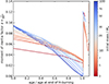 |
Fig. 2. Evolution of the moment of inertia factor of our SMC models. The abscissa is scaled in units of hydrogen burning times. |
Knowing a star’s rotational angular velocity, ω, we can calculate its rotational velocity at the equator, vrot, by multiplication with the star’s equatorial radius, Req, (de Mink et al. 2013). Since the star deforms due to rotation, the equatorial radius can be up to 1.5 times larger than the polar radius, Rp, which remains almost equal to the non-rotating radius. The ratio of the equatorial radius to the polar radius is a function of ω/ωcr ∈ [0, 1), where ωcr is the critical angular velocity of the model before it breaks up due to the centrifugal forces at the equator being larger than gravity. Thus, we have
 (5)
(5)
where  is the Eddington factor with the electron scattering opacity κ = 0.2 (1 + X) cm2/g (Kippenhahn et al. 2012). Following Rivinius et al. (2013), the radius ratio is
 (6)
(6)
Here, we simplified their expression. The critical rotational velocity is then given as vcr = ωcrReq. The rotational deformation does not lead to an earlier RLO, since we assume that before Roche-lobe filling the model’s rotation synchronises to the orbit, which leads to only mild radius ratios of a factor of about 1.1.
With this expression, we can trace the rotation of a stellar model over its evolution given an initial rotation and assume the same nuclear evolution as for a non-rotating single-star model. If the spin angular momentum, S = Iω, of the star is conserved (neither mass loss nor tidal torques), the angular velocity of the next time step is given by
 (7)
(7)
where we mark the quantities of the next time step with a prime and left those of the previous time step unmarked. We assume a rigid rotation, which is sufficiently fulfilled for main-sequence models, but after central hydrogen exhaustion stellar models clearly rotate differentially (e.g. Yoon et al. 2010; Schürmann et al. 2022). We were not able to trace differential rotation meaningfully with our means and, thus, we resigned from computing it thereon. In addition, the rotational decoupling process between core and envelope is not trivial, as Schürmann et al. (2022) showed.
If stellar winds become important, the change of spin angular momentum is
 (8)
(8)
neglecting deformation and assuming isotropic winds (Georgy et al. 2011, see however Hastings et al. 2023). The wind mass loss rate, Ṁ, can be calculated from our tabulated stellar models. Following Langer (1998), wind mass loss is amplified by rotation in form of Ṁamp = x Ṁ with
 (9)
(9)
for vrot/vcr ∈ [0,0.8]. Since this expression diverges for vrot/vcr → 1, we extrapolated it linearly by assuming the slope of Eq. (9) at x = 0.8, giving
 (10)
(10)
With this, we can write
 (11)
(11)
leading to
 (12)
(12)
In a binary system, the stars are subject to tides. To account for this we calculate the synchronisation time scales, τsync, of the models as Eq. (44) in Hurley et al. (2002) for hydrogen burning models with radiative envelopes (M > 1.2 M⊙) and Eq. (27) for hydrogen burning models with convective envelopes (M < 1.2 M⊙), see also Hut (1981). This gives us
 (13)
(13)
with Ω as the angular velocity of the orbit (e.g. Detmers et al. 2008). Recently, Sciarini et al. (2024) pointed out possible inconsistencies in this formalism. Equations (12) and (13) were applied one after another to yield the models’s angular velocity at the next time step. Since the orbital angular momentum of a model is much larger than its spin angular momentum, we can neglect changes of the orbit.
If this scheme leads to a model spinning over-critically, namely, ω > ωcr, we let the model lose additional mass at its equator. As the specific spin angular momentum there is ωR2 (noticing that in contrast to Eq. (8) the factor  disappears) and thus ΔS = ΔMωR2. We can assume that the mass loss to bring the model down to critical rotation is small, as Packet (1981) showed that large changes in stellar rotation require only small changes in mass, and therefore the change of radius is small, too, so we write ΔS = αMR2Δω. Equating these two expressions gives the additional mass loss to bring a model from rotating over-critically back to sub-critical rotation as
 (14)
(14)
It is generally assumed that accretion leads to the spin-up of stars. We calculated the accreted angular momentum depending on whether or not an accretion disk forms by calculating
 (15)
(15)
where a is the semi-major axis (Lubow & Shu 1975; Ulrich & Burger 1976; Paxton et al. 2015). If the accretor radius is larger than this value, we assumed ballistic accretion with a specific angular momentum of  and otherwise accretion from a Keplerian rotating disk at its equator and thus with a specific angular momentum of
  , where M and R refer to the accretor’s mass and radius. We assumed that a critically rotating accretor can keep accreting mass but limited its rotation to the critical value as the viscosity inside the disk transports mass inwards but transports angular momentum outwards (see Paczynski 1991; Popham & Narayan 1991; de Mink et al. 2013, for a discussion). An alternative view, where the accretion is limited by the accretors spin-up (Petrovic et al. 2005; Marchant Campos 2018), is investigated in Paper I.
3. Dependence of binary evolution on mass ratio, orbital period, and mass-transfer efficiency
Before we construct synthetic populations from our binary models, we need to understand how different initial masses, initial mass ratios, initial orbital periods and mass-transfer efficiencies affect the evolution of a binary in our code. Therefore we drew 104 binary models with uniform distribution in initial mass ratio, qi, (mass of the initially less massive star divided by the mass of the initially more massive star) and logarithmic initial orbital period, log Pi, for several fixed primary masses and mass-transfer efficiencies (with the non-accreted material carrying the same specific angular momentum as the accretor), and evolved them. We classified the evolutionary path either by the first SR that is produced or by a merger that happens before that, and colour the log Pi-qi plane according to the nearest model. For merging systems, we differentiated between the different reasons for that. In Fig. 3, we assumed an initial mass of 10 M⊙ and the online material contains similar diagrams for other masses. For simplicity, we assumed no SN kick.
In Fig. 3 we find that for low mass-transfer efficiencies most binaries can evolve to OB + NS systems (yellow) and, in case of high mass-transfer efficiencies, mergers dominate because of accretor swelling and subsequent L2 overflow (blue). At high orbital periods, we expect mergers due to the donor star developing a convective envelope (red) and at even wider orbits no RLO takes place at all (white). A large fraction of systems experience a Case BB/BC mass transfer (+-like pink hatching) except for wide systems, as the HeS is not able to fill such a large Roche lobe. Very close systems, which undergo Case A mass transfer, end up as OB + WD systems (green) since the mass of the stripped donor decreases with decreasing initial orbital period for Case A. If the initial mass ratio for Case A is too close to unity (orange) the slow phase of the mass transfer lasts so long that the accretor ends hydrogen burning, expands and fills its Roche lobe. So, a contact system is formed, which we assumed will merge fast. We discuss systems of initial mass ratios close to unity in Sect. A.
If we consider higher donor masses, we find that Case BB/BC RLOs soon disappear from the evolution as the HeSs do not grow to large radii for higher masses. The regions where mergers occur only shift slightly. Around masses of 20 M⊙ (online material) the donor becomes a BH (dark grey). For even higher masses we find that the Case A/B boundary shifts to higher orbital periods and that the merger region at q ≈ 1 becomes larger as the mass-lifetime exponent decreases.
Comparing these diagrams to the predictions by Schürmann & Langer (2024), we find about the same boundary between donor stripping and merger, as expected. In contrast to them, we find that our models merge at very low periods and high mass ratios and strip the donor (for high mass-transfer efficiencies) at high periods and high mass ratios. The differences arise, as Schürmann & Langer (2024) already predicted, since they neglected the evolution of the accretor, which we consider in the work presented here and which leads to the formation of contact systems as described above. Compared to Paper I, we predict mergers only at mass ratios far from unity if the mass-transfer efficiency is not too high. Only for very high mass-transfer efficiency, systems at intermediate mass ratios and high periods merge. The models of Paper I merge for intermediate mass ratios at low periods (independently for Case A and B), as the non-accreted material is gravitationally stronger bound, when the stars are close and the Roche radii are small, which makes the ejection of that material by their energy criterion harder. With our criterion, in close systems the donor radius is small when the RLO starts, which causes the thermal mass-transfer rate to be small and so the accretors do not swell and a contact is avoided. As we show in Sect. 5, this leads to strong differences for the period distributions of BeXB and OB + BH systems.
4. Influence of the mass-transfer efficiency on the synthetic populations
In this section, we generate synthetic binary populations, where the probability of drawing systems depends on the initial mass, initial mass ratio and initial orbital period distributions described in Sect. 2. We also employed the different kick scenarios and varied the mass-transfer efficiency from 10% to 100% in steps of 10% with additional values of 5%, 3%, 2%, and 1%. Each simulation contains 107 binary models and is scaled to a constant star-formation rate of 0.05 M⊙/a. We extracted the number of selected types of stars and binary systems (O-type stars, OB stars, OBe stars, BeXBs, and WR + O systems) and compare them to the observed numbers in Fig. 4.
The four panels in Fig. 4 are ordered in such a way that we can easily identify the impact of the initial binary parameters. The two panels on the left side have rather flat mass ratio distributions (κ ≈ 0.0) but those of the panels to the right are skewed towards more unequal systems (κ = −2.8 and −1.0). The upper panels both have a flat period distribution (π = 0), while for the two lower panels, close systems are preferred (π ≈ −0.5).
We calculated the number of systems with O-type stars by classifying all models with an effective temperature greater than 31 600 K as such. A margin of error can be derived from varying this number by one spectral class, namely, 30 350 K and 32 900 K (Schootemeijer et al. 2021), which is about 30%. The observed number of about 400 is the estimate corrected by completeness from Schootemeijer et al. (2021) and Shenar et al. (2024). The numbers of OB (hydrogen-burning model above 104 K) and OBe stars only includes stars with an absolute Gbp magnitude brighter than −3 (M ≳ 8 M⊙Schootemeijer et al. 2021), which is the completion limit of Schootemeijer et al. (2022). We used a distance modulus of 18.91 (Hilditch et al. 2005) and calculated the absolute Gbp magnitude following Schootemeijer et al. (2021). We classified all hydrogen-burning models as OBe stars if they spin faster than 0.95 times their critical rotational velocity (Townsend et al. 2004) and varied this number by including slow rotator and/or merger products. The observed numbers of OB and OBe stars are from Schootemeijer et al. (2022). We classified a model as a WR star if it is a HeS with a luminosity larger than 105.6 L⊙ (Shenar et al. 2020) and compared them to the four WR + O systems in the SMC (Shenar et al. 2016, 2018). (The other seven, seemingly single WR stars might have been formed through single-star evolution or in a later phase of binary evolution, and thus are disregarded in our analysis.) The margin of error is the Poisson counting uncertainty (i.e. ±2). Finally, we classified a model as BeXB, if it contains an OBe star according to the definition from above and an NS. 107 BeXBs are known in the SMC (Haberl & Sturm 2016)1 and the dimmest has a magnitude of 16.9.
For all initial distributions in Fig. 4, we identify a clear overproduction of O-type stars. This is not unexpected as this dearth was already discussed by Schootemeijer et al. (2021). The total number of bright OB stars is consistent with the observations and deviates by less than a factor of 1.5. Both quantities are almost independent of the mass-transfer efficiency. The predicted number of WR + O stars agrees with the distributions in Fig. 4 (top left, bottom left, and bottom right) in a wide range of mass-transfer efficiencies with the best match at low mass-transfer efficiencies. For the distribution in the top right, only mass-transfer efficiencies below 5% yield an agreement between simulations and observations. Thus, the number of WR + O systems is unaffected by reasonable variation of the initial period distribution but depends more on the initial mass ratio distribution. More extreme initial mass ratios lead to more mergers, reducing the number of systems. For all initial distributions, we find that the WR + O number decreases with increasing mass-transfer efficiencies. This comes from the larger merger area in Fig. 3 and the reduced lifetime of the accretor.
For the same reasons, we find fewer BeXBs at high mass-transfer efficiencies. It is only for very small mass-transfer efficiencies that we observe the opposite trend; in this case there is not enough mass transferred to the accretor, which then does not spin fast enough to become an OBe star. We predict most BeXBs for the no-kick scenario and least for the Hobbs scenario, as stronger kicks break up the systems more easily. An initial mass ratio distribution favouring low mass ratios (κ = −0.1 → −1, lower left to lower right panel in Fig. 4) decreases the number of BeXBs due to more systems merging and a period distribution favouring low periods (π = 0 → 0.5, top panels to bottom panels) increases the number of systems especially at high mass-transfer efficiencies as wide systems merge there more often than close systems (Fig. 3). A higher mass-transfer efficiency causes the magnitude of the dimmest BeXB to be smaller, as expected for a heavier accretor. This behaviour is independent of the initial mass ratio and initial orbital period distribution as it does not consider the number but only the occurrence of such systems.
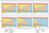 |
Fig. 3. Evolutionary outcome of our binary models with a primary mass of 10 M⊙ at the time when the first SR has formed, or when the system merges, as a function of initial orbital period (Pi) and initial mass ratio (qi) for six different mass-transfer efficiencies (ε). Each black dot represents one model system, and their total number in each plot is 104. We coloured the plane according to the result of the closest model (Voronoi diagram). We mark the boundary between RLO Case A and B by a black line. The occurrence of a later RLO with a HeS donor (i.e. Case BB or BC) is indicated by pink hatches. If the companion to a SR is not a MS star but a post-MS star, we mark it by orange cross-hatches in case it is H-rich (BSG/RSG), or by pink cross-hatches if it is H-poor (HeS). White regions are those with no RLO (top) or RLO at ZAMS (bottom). In grey areas, the outcome is not none of the above (often two SNe immediately after each other due to the final temporal resolution). |
For OBe stars, we find that their number increases with larger mass-transfer efficiency. While a lifetime effect might be present, here the assumed magnitude limit comes into play. A larger mass-transfer efficiency pushed more binaries with lower initial primary mass, which are preferred by the IMF, over the magnitude threshold than a lower mass-transfer efficiency. We find more OBe stars for steeper period distributions and flatter mass ratio distributions. For the Dunstall et al. (2015) distribution (top right) the curve showing the number of OBe stars is outside the range of the plot, meaning that this distribution underestimates the number of OBe stars by more than a factor of 10. Only the Sana et al. (2012) distribution (bottom left) reproduces the observed number of OBe stars when only considering fast rotators and only at very high mass-transfer efficiencies. When slow rotators are included, the two left panels of Fig. 4 produce the observed number of OBe stars with intermediate mass-transfer efficiencies. However, when doing this, one should also consider all OB + NS systems as BeXBs, which would lead to an overproduction of BeXBs. Another approach would be to vary the star-formation rate in such a way that it takes a higher value when the OBe star progenitors are born. However, it turns out that this is at the same age when the BeXB progenitors were born, so their number would be lifted, too. Figuratively speaking, both approaches mean that we cannot lift the OBe star curve without lifting the BeXB curve. Possible solutions could be to reduce the number of BeXBs again by assuming less reduced SN kicks or considering either merger products or single-star evolution as a channel for OBe star production. The above mentioned overproduction of OB stars simultaneous with the underproduction of OBe stars supports this finding.
In all figures, except Fig. 4 (top right), the line for the number of BeXBs and for the magnitude of the dimmest one meet at a mass-transfer efficiencies of 60–75%, close to the desired observed level. This suggests that during the formation of BeXBs the mass-transfer efficiency was rather high. The number of WR + O systems is best reproduced with low mass-transfer efficiencies, but only with a very large uncertainty, as indicated by the shading in Fig. 4. However, as we discuss in Sect. 6.3, there seem to be a preferences for low mass-transfer efficiencies at high stellar masses. This means that the mass-transfer efficiency might be a function of stellar mass. We assume in the following that the mass to be considered is the accretor mass, as we assume that this is the place in the system where the material is ejected. LMC stars are probably a better proxy for SMC stars than Milky Way stars, and so we choose the distributions of Sana et al. (2013, bottom right) as our fiducial set. In our model, the median initial mass of the accretor in WR + O systems is 35 M⊙, while it is 7 M⊙ for BeXBs. So, we varied the mass-transfer efficiency linearly between these two accretor masses, MA, which yields
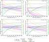 |
Fig. 4. Predicted number of selected types of stars and binary systems relative to the observed number (given in parentheses in the legend) as a function of mass-transfer efficiency. We show four different assumptions about the stars that become OBe stars – fast rotating accretors (solid line), fast and slow rotating accretors (dashed), fast rotating accretors and merger products (dotted), fast and slow rotating accretors and merger products (dash-dotted) – and three different assumptions about the SN kick – reduced kicks (solid), Hobbs kicks (dashed), and no kicks (dotted). The green line with labelling on the right side of the diagram shows the magnitude of the dimmest synthetic BeXB relative to the dimmest observed one (16.9). The pink shading indicated the uncertainty due to the low number of WR + O systems. The initial binary parameter distributions are flat (top left), according to Sana et al. (2012, bottom left), Sana et al. (2013, bottom right), and Dunstall et al. (2015, top right). |
 (16)
(16)
and we took the boundary values of 0.6 and 0.1 outside that range. The median mass of accretors in OB + BH progenitors turns out to lie with 15 M⊙ somewhere in between causing a typical mass-transfer efficiency of about 35% in such systems.
In Fig. 5 (top), we present the absolute number of OBe stars with HeS, NS and BH companions including those that were unbound from their NS in the SN. We assume the initial distributions from Sana et al. (2013). (See Fig. B.1 for other initial distributions.) We only consider HeS heavier than 2.55 M⊙, which is a rough limit between WD and NS formation. The numbers reach a maximum at mass-transfer efficiencies of 3%, since for larger values the accretors become heavier and thus live shorter and the lowest mass-transfer efficiencies depose not enough angular momentum on the accretor to become an OBe star. The number of of OBe + HeS does not drop as steeply as the others as it is, in general, the HeS, which evolved faster and ends the OBe + HeS phase. A stronger (weaker) SN kick reduces the number of OBe + NS = BeXB systems, while the number of unbound systems is increased (decreased). We find that the BH kick can unbind a substantial number of systems, reducing their number by a factor of two. We predict 10–200 OBe + BH systems. For a mass-transfer efficiency of 30%, which is the typical values one finds with Eq. (16), we predict 50 of them.
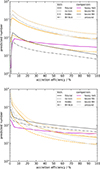 |
Fig. 5. Predicted number of OBe star (top) and regular OB star (bottom) companions indicated by colour and different kick scenarios indicated by line style as a function of mass-transfer efficiency for the initial distributions of Sana et al. (2013). |
In Fig. 5 (bottom), we show those OB-star models that are not rotating fast enough to be classified as emission-line stars. Again, the numbers shrink with larger mass-transfer efficiency. Towards low mass-transfer efficiencies, we find a sharp increase in the number of regular OB stars. This is because accretors are no longer spun up enough to become OBe stars. The OB + BH systems show a different slope than the other species. This may be due to the lower exponent of the mass-lifetime relation for massive stars. Furthermore the SN kicks affect these systems less than the OBe systems since non-OBe stars originate generally from closer and more strongly bound systems. We expect about 150 normal OB + BH systems.
5. The fiducial model with mass-dependent mass-transfer efficiency
In this section we present the properties of our fiducial simulation, namely, where the mass-transfer efficiency is a function of accretor mass according to Eq. (16), with the initial mass ratio and orbital period distributions of Sana et al. (2013) and the SN kicks as in Table 1. In the following, we often differentiate between OBe stars (main-sequence OB stars with Balmer emission lines) and regular or normal OB stars (main-sequence OB stars without emission lines). For this analysis, we rerun our fiducial model with 108 binary models.
5.1. Companions of OB stars after mass transfer in the SMC
In Fig. 6 we show the predicted fractions of companion types to our core-hydrogen-burning SMC models after mass transfer, as a function of their mass. This figure includes systems that become unbound during the SN event, but excludes merger products, single stars, and binary stars before interaction. We found four types of companions in such systems as well as systems unbound by the SN explosion, each occurring typically in a certain mass range. HeSs can be found over the whole mass spectrum. This is not surprising, as they are the immediate outcome of stable mass transfer. They make up about 20% of OB-star companions. For the lowest and the highest considered masses, this fraction reaches up to 30%. Fewer than half of their OB star companions are expected to be emission-line stars with a shrinking fraction towards higher masses.
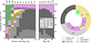 |
Fig. 6. Left: Predicted companion fraction of massive (M > 8 M⊙) main-sequence SMC stars in post-mass transfer binaries as function of their mass, including system in which the companion (in general a NS) was unbound during the SN, and excluding merger products. Models that we assumed to appear as emission-line stars are marked with black or white dots (depending on the background colour). Above each mass bin we give the total number of system in that bin. The total number of each companion type is given in the legend distinguishing between emission-line star (first number) and normal OB star (second number). Right: Absolute number of compact companions of OB stars (outer pie chart), and the assumed SN type of the NS progenitor (inner pie chart), predicted by our fiducial SMC population. |
Up to an OB-star mass of 14 M⊙, WDs can be found as companions, where most OB stars are expected to be emission-line stars. This is corroborated by the fact that most of these systems undergo a Case BB/BC RLO after core helium-exhaustion of the primary, during which the accretor is spun up a second time. NSs appear as companions for OB-star masses above about 8 M⊙ and dominate above about 12 M⊙. The NS companion fraction is largest around 15 M⊙ and drops to zero above about 24 M⊙. The ratio of normal OB + NS systems to OBe + NS systems increases towards higher masses. In contrast to the WDs, we predict a notable number of normal OB stars with NS companions, as the higher mass stripped stars avoid a mass transfer after core helium exhaustion. Many OBe stars spin down during core-helium burning of the stripped stars, which can be seen from the synthetic OB + HeS systems, as they are all assumed to rotate critically after mass transfer. Unbound systems have been found for the same OB-star masses as NS companions, as they share the same evolutionary past. Unbound OB stars have a larger OBe fraction than systems with NSs, which is probably caused by a larger probability of systems with high orbital periods, where tidal breaking does not play a role, to unbind during the SN explosion. We predicted 138 NS + OBe systems which we expect to appear as BeXBs, in good agreement with the observations. Additionally, we found 35 normal OB stars with NS companions.
Lastly, for OB stars above about 14 M⊙, we expect BH companions to start forming. They become the dominant companion type above around 18 M⊙ and reach a nearly constant fraction of around 80% for OB-star masses above 22 M⊙. Only for the highest considered OB-star masses (> 70 M⊙), the fraction of BHs decreases slightly. About 30% of BHs have an OBe companion and this number decreases with OB-star mass. The reasons are angular momentum loss by the stellar wind and the tides imposed by the BH and its HeS progenitor on to the star, which can be seen from their period distribution (see Sects. 5.3 and C). At such high masses, angular momentum loss by wind also becomes important, which can be seen by the decreasing number of OBe + BH systems for increasing OB mass. We predict for the SMC a total number of 142 OB + BH binaries for the scenario without a BH kick. 36 of them should have emission line companions. Additionally, we expect 106 normal OB + BH systems. This means that about 3% of all OB stars with an absolute magnitude brighter than −3, including pre-interaction systems, contain a BH, and around 6% of all OBe stars do. If we consider O-type stars only, these numbers become 10% and 50%.
Figure 6 (right) shows that bound OB + NS systems, unbound OB + NS systems, and OB + BH systems occur with roughly the same numbers. The dominant SN mode is CCSNe from a HeS progenitor (pink), which make up about 60% of all events. About 3/4 of them unbind the NS from the system. Systems with small helium core masses undergo an RLO Case BB/BC after core helium exhaustion and produce almost naked CO cores. As we assume that they experience smaller kicks, most of them remain bound. ECSNe, which have the smallest kicks (Table 1). In general, they do not lead to disruption and make up fewer than 1% of the unbound systems. In this scenario, without a BH kick, no BH is unbound from its companion star, and so all unbound systems released an NS. We discuss the effect of BH kicks in Sect. D.
5.2. Masses of OB stars and their companions
In Fig. 7 we show the predicted masses of the components of bound and unbound OB + NS systems and OB + BH systems. We find stellar masses (top row) from 9 to 100 M⊙. In different mass ranges, different companion types dominate. We find NS companions for stars with 9 to 22 M⊙ and BHs from 14 to 100 M⊙. Systems which broke up due to the SN kick follow the same patterns as NS systems, with slightly heavier OB stars as the former peak around 13 M⊙, while the latter reach their maximum at 12 M⊙. OB stars with BH companions have their mode at 20 M⊙.
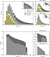 |
Fig. 7. Predicted masses of the components of massive binary systems after RLO and the formation of a SR. Top row: OB star masses coloured according to their companion type and marked with dots if we expect an emission-line star. The inlays in the upper right corners focus on the upper mass end. Bottom row: BH masses with dots in case of a OBe companion. Note: the vertical axis is logarithmic. Left: Total numbers. Right: Case A RLO (top) and B (bottom) separately. |
We can understand the mass distributions considering the assumed binary physics. We find the lightest NS progenitors to have an initial mass of about 10 M⊙, corresponding to a 3 M⊙ helium core at core hydrogen exhaustion. Thus, 7 M⊙ are lost from the donor during the mass transfer. The mass transfer efficiency is around 60% in this mass range and the minimum mass ratio for stable mass transfer is about 0.5 (see Fig. 3), which yields a lower limit of 5 M⊙ for the initial mass of the accretor, and therefore a minimum mass of 9 M⊙ for the OB star as seen in Fig. 7 (top). Similarly, the upper limit and the ranges of the BH companions can be understood.
Figure 7 (top right) shows Case A and B systems separately. We find that almost all regular OB stars evolved through Case A since in close orbits tidal forces are more efficient in braking the star. Systems tend to disrupt more frequently in Case B, which is due to the lower binding energy in wide orbits. In Case A systems, the mass distributions are slightly wider. This is caused by orbital-period-dependent donor mass after RLO (see Schürmann et al. 2024). Since the main-sequence models expand stronger for larger mass in our stellar model grid, the preference for BH systems to evolve through Case A is not surprising.
The lower panels of Fig. 7 show the mass distribution of the BH companions. They range from 4 to 32 M⊙ and show a slope dlog N/dMBH of about −0.05. The minimum BH mass derives from the minimum mass of a HeS to form a BH, which is 6.6 M⊙, and the BH formation prescription (Sect. 2) and thus it is 4.8 M⊙. The upper mass limit, about 30 M⊙, can be found similarly by taking away 50% of the initial mass of a 100 M⊙ star, our upper limit, to get the mass of the collapsing HeS.
The BH masses depict interesting differences between RLO Case A and B (Fig. 7, bottom right). While the mass distribution of Case A BHs shows the same slope as the total population, for Case B dlog N/dMBH is with −0.1 twice as large. We attribute this to the widening of the main sequence for increasing stellar mass. As already mentioned, BHs whose progenitor evolved through Case B prefer to have OBe companions, while those are rare for Case A BHs. For those, we find a large dip of OBe companions around 12 M⊙. It is unclear to us what causes it, but we expect it to have a limited effect as it would increase the number of emission line companions only by 4–5, if one would remove the dip by drawing a straight line over it. BHs that formed after a Case B RLO do not reach the same maximum mass as those from Case A because our stellar models above 80 M⊙ did not evolve beyond central hydrogen exhaustion.
In Fig. 8 (second row left), we show the combined mass distributions for OB + BH systems (see also Sect. C). This distribution can be described as being framed by four lines. At first, there are the upper and lower BH masses, as discussed previously. As we have shown in this section, we can divide the BH mass by 0.36 to estimate its initial stellar mass. Secondly, the population is limited to the left by a diagonal line following q ≈ 1. These systems stem from those with the initially most extreme mass ratios of about 0.3. Take for instance the upper left corner with MBH ≈ 30 M⊙ and MOB ≈ 30 M⊙. The initial BH progenitor mass was about 100 M⊙ and the initial accretor mass about 25 M⊙, since the mass-transfer efficiency is small at high masses. The systems in the lower left corner on the other hand (MBH ≈ 6 M⊙ and MOB ≈ 10 M⊙) had initial masses of about 15 M⊙ and 6 M⊙ due to the higher mass-transfer efficiency.
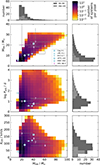 |
Fig. 8. Predicted properties of OB + BH systems. The left panels shows the number of systems in the OB mass–BH mass plane (second row), OB mass–orbital period plane (third row), and OB mass–OB velocity semi-amplitude plane (fourth row) in logarithmic colouring and the other panels are projections of that onto one axis, i.e. the distribution of OB masses (first row left), BH masses (second row right), orbital periods (third row right), and OB star velocity semi-amplitudes (fourth row right), where emission-line stars are marked by white dots. We also show the properties of all dynamically confirmed OB + BH systems in the local group and of the WR + O systems in the SMC with WR masses as BH masses. |
The systems at the right side of Fig. 8 (second row left) are bounded by a line of q ≈ 0.2…0.3 and come from systems with a mass ratio initially close to unity. Here, however, effects of Case A mass transfer come into play. Take, for example, a system with initial masses of 15 M⊙ and 14 M⊙. If the donor loses half of its mass of which about a third (Eq. (16)) is gained by the accretor, the OB star would have 16 M⊙, but the diagram shows accretors as heavy as 22 M⊙ in the lower right corner of the population. This is due to the fact, that donors which evolve through Case A mass-transfer can lose more than half of their mass, especially if a Case ABC mass transfer strips them even further, reducing the mass of the BH and increasing the mass of the OB star. For the density of systems per pixel in Fig. 8 (second row left) we note, that the number of systems decreases for larger BH masses, but is fairly constant for varying OB-star masses. The former derives from the IMF and the latter from the near flat initial mass ratio distribution. This means it is more likely to find a 30 M⊙ OB star with a 15 M⊙ BH than with a 30 M⊙ BH, but it is about equally likely for a 20 M⊙ BH to have a 30 M⊙ and a 50 M⊙ OB companion.
Figure 9 shows the predicted OB + BH population in the Hertzsprung-Russell diagram (HRD). It is expected that fast-rotating stars will redden due to the von Zeipel-theorem. We are not able to include this effect in our analysis as our models are fixed and rather show the non-rotational effective temperature. The OB stars have luminosities from 104.5 L⊙ to 106.5 L⊙ and display temperatures from 25 kK to 50 kK corresponding to O- and the earliest B-type stars. For the most massive companions, the main-sequence broadens a lot leading to a lowest effective temperature of 10 kK. Their contribution is, as we can see in the upper panels, negligible. The HRDs for the predicted OB + NS systems are provided in Sect. C.
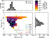 |
Fig. 9. Predicted HRD positions of OB stars with a BH companions in logarithmic colouring together with selected model tracks and the ZAMS. We include values of all observed OB + BH systems and the O-type star of SMC WR + O systems (see Fig. 8 for the symbols). The panels on top and on the right show the temperature and luminosity distributions with predicted emission-line stars highlighted by dotting. |
To make a meaningful comparison of our simulations with the observations, we estimate the V-band magnitudes of our OB-star models by using the recipe from Schootemeijer et al. (2021), which is based on Dotter (2016) and Choi et al. (2016), to calculate magnitudes from luminosity and effective temperature. We show the results in Fig. 10. There, the slope of the expected OBe stars dlog N/dmV of about 0.55 until a magnitude of 12, where their number drops significantly, while the number of all post-RLO systems continues to follow the same slope. A difference already appears around mV = 14. The magnitudes we found for OB + NS binaries reach from 13 to 17 with a maximum of around 15.5. The distribution is skewed towards dimmer stars. BeXBs are slightly more common at larger magnitudes. BHs can be found around stars brighter than mV = 16. Their distribution is flatter and less skewed than the OB + NS distribution.
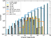 |
Fig. 10. Predicted and observed distribution of V-band magnitudes. The blue bars show the magnitudes of all OB star models (i.e. with HeS, WD, NS, and BH companion and unbound systems) after stable mass transfer. OBe candidates are marked with dots. As observations we show the SMC OBe magnitudes distribution (blue line) from Schootemeijer et al. (2022), the magnitudes of BeXBs (orange line) from Haberl & Sturm (2016)2, SMC X-1 (grey dashed line) and J0045-7319 (brown line). |
Living version: https://www.mpe.mpg.de/heg/SMC
5.3. Orbital parameters
For the systems that remain bound after the formation of the SR, we can analyse their orbital properties, namely, the orbital period, Porb, eccentricity, e, and orbital velocity semi-amplitude of the OB star, expressed as
 (17)
(17)
Here, a is the semi-major axis. Figures 8 and 11 show these orbital properties of our OB + BH binaries. In the bottom left panel of Fig. 8, we can see that systems with masses around 20 M⊙ and velocity semi-amplitudes from 25 to 150 km/s are preferred. Only the widest systems, those with low orbit velocities, become OBe stars. The upper right corner is empty as their progenitors would have initially overfilled their Roche lobe. No systems can be found at high velocities and low masses because the donor after Case A is too light to form a BH. The centre right panel of Fig. 11 shows a somewhat narrow relation between orbital period and velocity semi-amplitude, which is due to Kepler’s law. In the centre left panel of Fig. 8 the combined distribution of orbital period and OB-star mass is shown. Both quantities are highly skewed and peak at low values. Towards high masses and periods a wide plane can be found. The upper right corner is empty because such systems are very rare due to the initial distributions. Systems with low periods and high masses are avoided as such systems would overfill their Roche lobe initially. Finally, the bottom centre panel of Fig. 11 depicts orbital period and eccentricity. The eccentricity only assumes values between 0.05 and 0.2 and strongly peaks at 0.1. The reason is our BH formation formalism. As 20% of the helium envelope is lost, the BH progenitor loses some of its momentum, which translates to a non-zero eccentricity (Tauris & Takens 1998). Varying the mass loss or imposing a kick on the BH would change the resulting eccentricity dramatically. We note, however, that our prescription does not account for the continuous circularisation of the orbit due to tides after the SN, so the real eccentricity may be lower. Nevertheless, the eccentricity distribution of wide OB + BH systems could be a probe for BH kicks.
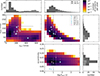 |
Fig. 11. Predicted properties of OB stars that have BH companions with measurements of all dynamically confirmed OB + BH systems in the local group and of the WR + O systems in the SMC. The main panels shows the number of systems in the rotational velocity-velocity semi-amplitude plane (first column, second row), orbital period-velocity semi-amplitude plane (second column, second row), and eccentricity-velocity semi-amplitude plane (second column, third row) in logarithmic colouring and the other panels are projections of that onto one axis, i.e. the distribution of OB rotational velocities (top left), orbital periods (top centre), OB star velocity semi-amplitudes (centre right), and eccentricities (bottom right), where emission-lines stars are marked by white dots. |
We show a combined histogram of rotational and orbital velocity of OB + BH systems in Fig. 11 (centre left). We find that the OB + BH populations divides clearly in two sub-groups. The somewhat larger group can be found at low rotational (< 200 km/s) and medium to high orbital (> 50 km/s) velocities. These systems evolved through Case A RLO and are normal OB stars. Systems with high rotational (> 300 km/s) and low orbital (∼50 km/s) velocities form the second group and are in general emission-line stars. This has an important implication for the observational search for BHs, namely that on one hand high radial velocity variations in SB1 systems and on the other hand that OBe stars are a predictor of BH companions.
The orbital properties period and eccentricity of OB + NS binaries are shown in Fig. 12. We do not treat mass ratio and orbital velocity here because the NS mass is strongly confined and the OB stars’ velocities are very low due to the low NS mass, see however Fig. C.1. The centre panel shows a 2D histogram of orbital period and eccentricity. The eccentricities follow a very broad distribution covering all values from 0 to 1 and the periods’ mode is, as discussed above, between 10 and 100 d. The combined distribution has accordingly a large main feature at these values. A notable exception is a preference for large orbital periods at high eccentricities and an avoidance of high eccentricities at low orbital periods. This is not surprising as this would lead to Roche-lobe overfilling periastron distances. While emission-line stars are more frequent at large orbital periods, we find no dependence on eccentricity.
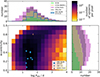 |
Fig. 12. Predicted orbital properties of OB + NS systems with observations of the SMC BeXBs, SMC X-1, and J0045-7319. Centre: Orbital period-eccentricity plane. Top: Orbital period coloured by SN type. Right: Eccentricity coloured by SN type. |
In the top and right panels of Fig. 12, we show the period and eccentricity distributions coloured according to the SN type. CCSNe from a HeS, CCSNe after a Case BB/BC RLO, and ECSNe have slightly different typical orbital periods, increasing in that order. This means systems with a stronger kick end up with lower orbital periods, which may sound counter-intuitive but can be explained by wider orbits being more likely to unbind than close orbits or by the different initial parameter spaces of different SN types. Furthermore, CCSNe from HeS progenitors are the only species that yield a notable amount of regular OB stars as tidal breaking before the SN is only possible here. In the case of a CCSN after Case BB/BC RLO, the OB star was just spun-up again, and systems that undergo an ECSN and are close enough for effective tidal braking also experience such a mass transfer. The eccentricities of systems that evolved through ECSNe show the smallest eccentricities and those which experienced a CCSN from a HeS the largest. This also reflects the magnitude of the SN kick as higher kick velocities lead to more eccentric systems. As mentioned above we did not employ continuous tidal induced circularisation of the orbit which may affect the eccentricity distribution.
5.4. Systemic velocity
Because a SN kick changes the momentum of the system, we are able to predict the space (centre of mass) velocity  of our OB-star systems and ejected OB stars as we do in Figs. 13 and C.5. We find that NS systems (yellow) have the broadest distribution from 0 to up to 100 km/s. Even more striking is that this distribution is bimodal with one narrow maximum at 10 km/s and a wide one at 40 km/s. Inspecting the upper left panel we see that the first peak comes from ECSNe and CCSNe of a Case BB/BC donor. The second peak comes exclusively from CCSNe with a HeS progenitor, as they have the highest kick velocities, which lead to high space velocities. CCSNe preceded by Case BB/BC RLO and ECSNe end up with lower space velocities, which is in agreement with the strength of their kicks. NS systems with the largest space velocities do not tend to be OBe stars. This is due to the fact that the pre-SN orbital velocity leaves an imprint on the space velocity (Tauris & Takens 1998). Thus, we can assume that they come from initially close binaries which explains the absence of fast rotation. The panel on the top right of Fig. C.5 supports that Case A produces faster systems.
For unbound systems (grey contour in Fig. 13) we find the most common space velocity of the OB star just above 10 km/s. They again reach up to almost 100 km/s but do not have the bimodality of their bound counterparts. BH systems also show a unimodal distribution, but with lower velocities (peak at 20 km/s), since we do not assume any BH kicks. Their velocities are, as well as the eccentricities, caused by the mass loss during BH formation. With our adopted assumptions, BH systems do not break up.
In the centre of Fig. 13, we show a 2D histogram of spacial and rotational velocities of all OB + SR systems, whether bound or unbound. We find similarly to Fig. 11 (centre left) two populations. First, there are systems with high rotational (> 300 km/s) and relatively low spatial velocity (peak at 10 km/s), which are the Case B and wide Case A systems. Then there are systems with low rotational (∼100 km/s) and higher spacial velocities (mode at 20 km/s). These are the narrow Case A systems where tidal locking is relevant, which inherited their fast orbital velocity as systemic velocity.
6. Discussion
In this section, we compare our results with observations (Sect. 6.1), with Paper I (Sect. 6.2) and previous works (Sect. 6.3). The main uncertainties of our simulations are discussed in Sect. D.
6.1. Comparison with observations
In this section, we compare our predicted distribution to observations of SMC systems and suitable proxies. We focus mostly on systems with BH or NS companions and their directly observable properties.
6.1.1. BH systems
No OB + BH system has been observed thus far in the SMC. Therefore, we relied on OB + BH systems observed in the local group and WR + OB systems, which are believed to evolve to OB + BH systems (Langer 2012), as proxies. The OB + BH systems in question are Cyg X-1 (Orosz et al. 2011; Miller-Jones et al. 2021), LMC X-1 (Orosz et al. 2009), M33 X-7 (Orosz et al. 2007; Ramachandran et al. 2022), VFTS 243 (Shenar et al. 2022a), and MWC 656 (Casares et al. 2014, the true nature is under debate, see Rivinius et al. 2024 and Janssens et al. 2023). For the WR + O systems, we rely on Shenar et al. (2016) and Shenar et al. (2018) and references therein. We aligned all analysed quantities by considering their inclination. The BH systems exist in environments with higher metallicities than the SMC, which has effects on the mass limit for BH formation, the BH mass, and the OB star mass and rotation by wind mass loss and wind angular momentum loss (Langer 2012; Tauris & van den Heuvel 2023).
In Fig. 8, we can see that our predictions and the observed masses cover the same ranges. We treated the WR mass (Schootemeijer & Langer 2018) as BH mass assuming the WR collapses completely to a BH. It is possible that some material is ejected and the total mass is reduced by gravitational binding energy, see Sect. 2. MWC 656 is at the extremely low mass end of both components, assuming it is a BH system. However, we find that the observations are roughly equally distributed over the predicted area. This is not surprising as the selected observations are biased towards higher masses. First, massive stars are brighter and more likely to observe, and second WR + O systems are the OB + BH progenitors with the highest masses and far more likely to identify observationally than HeS + OB systems, where the HeS is not a WR.
In Fig. 8 (bottom), we find the observed systems to cluster around a velocity semi-amplitude of 100 to 150 km/s. The reason may be the difficulty in observing systems with lower values. In the top centre panel of Fig. 11, we find that the observations follow the shape of the predicted population. Only MWC 656 lies in the region where we expect OBe stars (high period, low orbital velocity) and it is the only known BH + OBe candidate. As predicted, we found a typical orbital period of around 10 d.
The bottom centre panel of Fig. 11 shows the predicted the OB + BH systems’ eccentricities to range from 0.05 to 0.20 but the observed OB + BH systems have values clearly below this, with the sole exception of MWC 656. The reason may be tidal circularisation in close orbits, no mass and energy loss during the BH formation, a kick, as post-SN eccentricities below about 0.06 can only be produced by a kick (Tauris & Takens 1998), or our BH formation scheme overestimates the mass ejection during BH formation process. Even more interesting is that the WR + O systems from the SMC have small, but non-zero eccentricities (Foellmi et al. 2003; Shenar et al. 2016, 2018), while we would expect a perfectly circular orbit after RLO.
All observed BH/WR + OB systems (but MWC 656) are observed to have relatively similar orbital (∼120 km/s) and rotational velocities (∼200 km/s) of the OB star (Fig. 11, centre left). These observations are close to the our predicted subpopulation of BH + OB systems with slow rotation. However our synthetic population rather has with about 100 km/s a most likely rotational velocity that is half as large as observed. This may be due to an overestimate of tidal, wind braking in our models or due to a different stellar structure. We can conclude that these systems likely evolved through Case A mass transfer. MWC 656 however seems to belong to the OB + BH sub-population at high rotation. Indeed this system harbours an emission-line star matching the predictions. Thus MWC 656 might be the tip of the iceberg of yet undiscovered BH + OBe systems.
While all other BH/WR + OB systems can be observed with temperatures and luminosities in good agreement with our predictions, our model cannot explain the location of MWC 656 in the HRD (Fig. 9). This is because the Be star in MWC 656 is about 8 M⊙ but the predicted lightest OB star with a BH companion is about 12 M⊙. This may be due to uncertainties in our BH formation criterion or an overestimate of the mass-transfer efficiency in long-period BH-forming systems. On the other hand, as already mentioned above, the BH nature of MWC 656 is challenged by Rivinius et al. (2024) and Janssens et al. (2023), who find that MWC 656 harbours a subdwarf instead of a BH.
6.1.2. BeXBs, SMC X-1 and J0045–7319
Haberl & Sturm (2016)2 reported 107 BeXBs in the SMC. They give V-band magnitudes for 102 and orbital periods for 54 of them. Townsend et al. (2011), Coe & Kirk (2015), and Townsend et al. (2017) listed the eccentricities for eight BeXBs. Next to the BeXBs two other systems with a NS are found in the SMC. These are the super-giant X-ray binary SMC X-1 (van der Meer et al. 2007) and the pulsar/B-type star binary J0045–7319 (Bell et al. 1995; Kaspi et al. 1996; Manchester et al. 2005). Magnitude, orbital period and eccentricity are well known for them, which we show in Figs. 10 and 12.
The V-band magnitudes of BeXBs cover the same range as our simulation (Fig. 10), but the distributions have slightly different shapes. SMC X-1 lies at the bright end of our distribution and J0045–7319 at the dim end, while we would have rather expected such systems without emission lines over the whole range of magnitudes.
The orbital period distribution of BeXBs behaves with values above 10 d like the synthetic one (Fig. 12). Both samples spread out over several decades and show a clear maximum. The differences, especially the large number of BeXBs with periods between 56 and 100 d may be due to sampling. The period of J0045–7319 is close to the mode of the model’s; however it is not an OBe star like almost all of our systems at such a period. SMC X-1 has with 3.89 d the shortest orbital period. At such short periods we predict that the OB star does not show emission lines. Indeed, SMC X-1 is a super-giant X-ray binary.
If we consider eccentricities, we find a notable difference between our work and the observations. While we predict an almost flat distribution for the BeXB, the observations range only up to 0.5. This may be due to an observational bias against high eccentricities. The high eccentricity of J0045–7319 and the near zero one of SMC X-1 fit our model. In Fig. 12 (centre) we find that all observations lie where we predict the largest density of systems. The only exception is SMC X-1, which may be explained by our ignorance towards tidal circularisation. The mass ratios of SMC X-1 (0.068 ± 0.010) and J0045–7319 (0.16 ± 0.03) are at the edges of our predictions (Fig. C.1). The deprojected rotational velocity of the optical counterpart of J0045–7319 is 163 ± 21 km/s and fits to the predictions for normal OB star in Fig. C.2. The LMC BeXB system A0538-66 (Porb = 16.6 d, e = 0.72 Rajoelimanana et al. 2017; Ducci et al. 2022) is covered by our synthetic systems in Fig. 12.
6.1.3. Be and Oe stars
Schootemeijer et al. (2022) photometrically identified the complete population of massive OBe stars in the SMC. We show their magnitude distribution in Fig. 10. When compared with our synthetic OBe star population (the blue bars with black dots) we find that the two slopes agree well for intermediate apparent magnitudes (13–16). However, we underestimate the number of OBe stars by a factor of about two for each magnitude bin, as discussed in Sect. 4. Similarly, our models predict an OBe fraction  (apparent magnitude brighter than 16) of about 13% (Fig. 4, bottom left panel), whereas Schootemeijer et al. (2022) find 31% and Dallas et al. (2022) report 34%.
Shenar et al. (2024) found that 20 out of the 159 O-type stars that they analysed were Oe stars (13%). The value of Dallas et al. (2022) is similar (17%) This suggests that there are approximately 50–60 Oe stars in the entire SMC based on 400 O-type stars in total (Sect. 4). Our models predict about 70 such stars, however with an Oe fraction of about 5%. While the discrepancy for OB(e) stars stems from the underproduction of OBe stars, the mismatch for O(e) stars comes from the overestimation of O-type stars (see Sect. 4).
6.1.4. Spatial velocities
In Fig. 13, we have added local transverse velocities of 163 isolated SMC OBe stars from Dorigo Jones et al. (2020) and Phillips et al. (2024). For most of these observations the binary status is unknown, but since Bodensteiner et al. (2020) and Dallas et al. (2022) found evidence that such systems are post-interaction systems, we assume this and compare them with our OB + SR systems (including unbound accretors). The observations likely also contain OB + HeS systems for which we expect no local spatial velocity as they did not undergo a SN. 17 of them have a counterpart in the BeXB table of Haberl & Sturm (2016) wherefore we highlight them as well as SMC X-1. Dorigo Jones et al. (2020) and Phillips et al. (2024) also provide rotational velocities for 63 of their systems. Notice that the observations are projected velocities but our simulations are not.
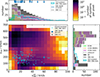 |
Fig. 13. Predicted space velocities and rotational velocities of OB stars with bound and unbound NS and BH companions with observations of the transverse velocities of isolated SMC OBe stars (blue line and small dots), BeXBs (large blue dots), and SMC X-1 (grey). The median error of the transverse velocities is 23 km/s. Centre: space velocity–rotational velocity plane. Top: space velocities coloured by SN type. The part of the histogram within the grey line indicates the unbound systems. Right: rotational velocities coloured by SN type. |
The velocity range of observed and simulated systems agree well, while the shapes of the distributions are different (Fig. 13 top). Our data are more strongly skewed towards lower velocities, which one would rather expect from the observations due to projection effects. A possible explanation is an observational bias against slow-moving systems and the relatively large uncertainties. (The median error of the local transverse velocity is 15 km/s.) The BeXBs on the other hand seem to follow the simulated distribution more closely as they cluster between 10 and 20 km/s. However, the system with the largest observed projected velocity is already moving as fast as the fastest (not projected) synthetic BeXBs. SMC X-1 is with 27 ± 26 km/s in agreement with our OBs + NS systems.
In the centre panel of Fig. 13 we find that the bulk of the observations show lower rotational velocities than we predict. All of the observed OBe stars lie in the part of the diagram where we predict normal OB stars. The not considered inclination of the observed system is not able to account for this. However, the observations may underestimate the rotational velocity at the equator as this region cools by the von Zeipel-theorem and thus dims (Townsend et al. 2004). We also may have underestimated the effects of tidal and wind braking.
6.2. Comparison with detailed binary models
In this section we compare our results to Paper I, which is a companion study with the same aims but a different approach. While we use a rapid binary population synthesis code to generate a large range of model populations, Paper I uses a given set of detailed MESA binary models. In addition, the major differences between the two works are, first, that our models accretion during RLO is not limited to the achievement of critical rotation of the accretor but is normalised to the observed number of BeXBs and WR + O systems. Second, Paper I uses a luminosity criterion to decide whether an RLO is stable or leads to a stellar merger, while we rely on the occurrence of an L2 overflow due to the swelling of the accretor. The major consequence is that the qi-log Pi-diagram of the two approaches look very different (our Fig. 3 and online material and their Figs. 2, A.1, and A.2). While in Paper I, the region where donor stripping occurs has the shape of two triangles with stable mass transfer up to smaller mass ratios at high orbital periods, in our work the transition between Case A and B is continuous and if systems merge they tend to be those at high orbital periods and mass ratios away from unity. These two mass transfer criteria end up producing very different OB + BH populations. Paper I predicts a large fraction of long-period binaries associated with fast-rotating main-sequence companions, but our predicted OB + BH binaries are dominated by close systems with normal OB stars
Thanks to a direct comparison of our Fig. 6 and Fig. 6 of Paper I, we can see that those authors predicted an overall smaller number of OB + SR systems. Also, their number in each mass bin is smaller than ours. The different companion types are also differently distributed over the OB-star masses. Their OB stars up to 8 M⊙ and 30 M⊙ have WD and NS companions, respectively. The NSs with such massive companions had to have evolved via Case A mass transfer, which can cause differences in its final fate, based on MESA models of the internal structure of the stripped star in detail. On the other hand, stars as light as 6 M⊙ harbour NSs and BHs in their study, while our lowest masses are 8 M⊙ and 14 M⊙ due to the difference in the mass-transfer efficiency and mass-transfer stability3. The ratio of OB + NS to OB + BH systems of Paper I is lower than ours because their merger fraction for NS-forming systems is much higher than ours. Furthermore, we predict more Case B mergers and fewer Case A mergers, resulting in a lower ratio of OBe to normal OB stars than that in Paper I and a weaker dependence of the OBe-to-OB fraction on OB mass for OB + BH and OB + HeS systems, which is probably due to the treatment of wind angular momentum loss (see Sect. D).
An important consequence of the merger criterion of Paper I is the bi-modality of the orbital period (their Fig. 8), which is not present in our Fig. 12. The range of orbital periods is similar, nevertheless. While the systems at low orbital periods may not appear as BeXB and are rather X-ray quiet (Paper I), this prediction could be tested. The current data seem to support our approach.
In our model, the mass-transfer efficiency is only a function of accretor mass; however, in Paper I, we found that it can depend on both masses and the orbital period. This may be the cause of several differences between our results, such as the larger spread of OB-star masses for a fixed BH mass (our Fig. 8 and their Fig. 11) and the larger range of luminosities of NS and BH companions and stronger overlap of the populations (our Fig. 9 and their Fig. 4) in Paper I. Overall, Paper I predicts fewer massive stars in OB + BH systems due to their lower mass-transfer efficiency. This also causes that our predicted mass ratios of OB + BH systems to be smaller than in Paper I.
An interesting and testable difference can be found in our Fig. 8 and Fig. 11 of Paper I. We predict the lower left corner in the MOB-Porb diagram to be much stronger populated than Paper I does. In our Fig. C.4 and Fig. G.5 of Paper I, we can identify, accordingly, the lack of close normal OB + BH systems. It may be explained by the fact that our merger criterion lets more systems with initially short periods and extreme mass ratios survive at low (∼15 M⊙, the lowest BH progenitor initial mass) initial donor masses. If these close and light OB + BH binaries exist, they may produce observable X-ray emission (Sen et al. 2024).
There are also differences in the rotational velocities of OB stars predicted by the two studies as can be seen in our Fig. C.2 and Fig. G.7 of Paper I. The population at low rotational velocities is missing in Paper I, which could either be due to the different implementation of stellar rotation and angular momentum loss by tides and winds (see also Sect. D) or due to the merger criteria. We also find that the high rotation peak is broader in Paper I, which is probably due to the implementation of rotational evolution. In our work this peak is only very weak for the BH companions. Paper I also has a smaller number of normal OB + NS systems and Case B systems do not have vrot/vcr below 0.8 in general.
For the OB + NS systems, we find that Paper I predicts a slightly flatter eccentricity distribution but the tendency to have higher eccentricities for the largest periods remains (our Fig. 12 and their Fig. 9). For the SN types, we find about the same tendencies with fewer CCSNe preceded by Case BB/BC in Paper I; this might be caused by the ability of the HeS to expand due to the presence of a hydrogen shell. It is also interesting to note that Paper I finds much fewer OB + NS systems with velocity semi-amplitudes above 40 km/s (our Fig. C.4 and their Fig. G.6).
6.3. Comparison with earlier work
Over the last three decades, many population synthesis studies of X-ray binaries and/or OBe stars (e.g. Meurs & van den Heuvel 1989; Waters et al. 1989; Pols et al. 1991; Tutukov & Yungelson 1993; Iben et al. 1995; Dalton & Sarazin 1995; Portegies Zwart 1995; Portegies Zwart & Verbunt 1996; van Bever & Vanbeveren 1997; Terman et al. 1998; Raguzova & Lipunov 1998; Van Bever & Vanbeveren 2000; Raguzova 2001; Lü et al. 2011; Shao & Li 2014; Zuo et al. 2014; Renzo et al. 2019; Vinciguerra et al. 2020; Schootemeijer et al. 2022; Misra et al. 2023; Liu et al. 2024; Rocha et al. 2024; Ge et al. 2024; Vargas-Salazar et al. 2025) have been conducted. While many of them have focussed on the X-ray output, we discuss those focussed on aspects of binary evolution in the present work.
A popular approach in the past was to use a mass ratio dependent mass-transfer efficiency, as Pols et al. (1991), Portegies Zwart (1995) or Portegies Zwart & Verbunt (1996) did. Typical assumptions are a high efficiency for systems with mass ratios close to unity and low values for rather unequal systems with a narrow transition zone. This description is in general not able to reproduce the mass (or spectral type) distribution of BeXBs, as B-type stars as light as 2 M⊙ are predicted. SN kicks are not able to regulate that sufficiently (Portegies Zwart 1995). Rephrasing this criterion into a thermally limited accretion (Portegies Zwart & Verbunt 1996) leads to the same problem. Numerous studies (e.g. Pols et al. 1991) have introduced an ad hoc minimal mass ratio for stable mass transfer of about 0.3 to 0.5 to remove systems with light companions. Portegies Zwart (1995) identified with the specific angular momentum of the ejected material a further key parameter, which they used to regulate which binaries evolved to BeXBs. They found that the larger the specific orbital angular momentum of the ejected material, the larger is the minimal mass ratio for donor stripping. This was confirmed by van Bever & Vanbeveren (1997) and Terman et al. (1998). More recently, Shao & Li (2014) tested three models within the stable RLO channel to examine the formation of OBe stars by binary interaction. They could best explain the observed mass and orbital period distribution of OB + NS systems neither with the rotation-limited accretion model nor with the thermally limited accretion model but only with the model with 50% mass-transfer efficiency, for which the authors found in contrast to the other two models no physical motivation. Lastly, Vinciguerra et al. (2020) studied a combination of three fixed mass transfer efficiencies and three models for the loss of angular momentum. Each combination resulted in a certain minimal mass ratio for successful donor stripping. With that, they confirmed the earlier findings about the minimum mass ratio, the need for a moderate mass-transfer efficiency and notable angular momentum loss from the system. All these findings are in line with the results of our study, and furthermore, we are able to connect the minimal mass ratio for stable mass transfer with the mass-transfer efficiency by a physical mechanism. In general, our results for distribution functions of parameters of BeXBs agree with previous works and differences can easily be explained by the underlying physics.
Several studies address the number of BeXBs. Vinciguerra et al. (2020) found that their mechanism under-predicts their number and needs to invoke a time-dependent star formation rate. They need to do this since many of their systems were disrupted during the SN because the authors do not use reduced SN kicks for stripped stars as we do. Shao & Li (2014) and Renzo et al. (2019) report that for the same reason there is a larger ratio between unbound and bound NS than we do. That SN kicks regulate the number of BeXBs was also found by Portegies Zwart & Verbunt (1996), Raguzova & Lipunov (1998) and Renzo et al. (2019). Raguzova & Lipunov (1998) further showed that the magnitude of the kick does not change the shape of the orbital period distribution and only slightly changes the shape of the eccentricity distribution.
In Sect. 4 we report evidence that binary evolution alone cannot account for the large number of OBe stars in the SMC. The literature shows no consensus on the question of how important this channel is for their formation. While, for instance, Pols et al. (1991) found that no more than 60% of them can come from the binary channel, Shao & Li (2014) can explain all OBe stars by binary evolution. Hastings et al. (2020) found that single-star evolution is not able to explain the observed number of OBe stars in open clusters, but binary evolution might be able to (Hastings et al. 2021). At this point, neither single star evolution nor binary evolution alone can explain the observed amount of OBe stars.
We identified further characteristics shared by our and previous studies. In general, 20% of mass gainers of all masses are predicted to have a HeS companion (Portegies Zwart 1995; van Bever & Vanbeveren 1997). Several further studies (e.g. Tutukov & Yungelson 1993; Terman et al. 1998; Shao & Li 2014) found that the common envelope channel is not relevant for the formation of BeXBs. Tides are the reason why systems with small orbital periods do not evolve to BeXBs (Raguzova & Lipunov 1998) and circularise close systems, which we neglected (Terman et al. 1998; Shao & Li 2014). Renzo et al. (2019) identified that the minimum mass ratio for successful donor stripping and the mass-transfer efficiency impact the velocity distribution of unbound stars.
Several studies have made predictions about the yet unobserved OBe + BH population. Raguzova & Lipunov (1999) predicted orbital period and eccentricities in agreement with our results, even though they require the BH progenitors to have initial masses of at least 50 M⊙. Shao & Li (2014) predicted OB(e) + BH binaries for their rotationally limited and their semi-conservative model but not for their thermally limited accretion model as in the latter the OBe stars become too massive. In the former two models, the OBe + BH populations have different OB-star masses. They offer a good agreement with our model (e.g. Fig. 8) as our effective mass-transfer efficiency for BHs lies in between their two models. Their ratio of OBe + NS and OBe + BH systems is larger than ours as they do not consider O-type stars as emission-line stars. Shao & Li (2019) predict the Galactic population of BHs with normal star companions assuming a rotationally limited mass-transfer efficiency. Their model B, which is similar to our scenario with BH kicks, yields relatively similar results, while differences in the companion masses are smaller by a factor of 2 (probably due to the lower mass-transfer efficiency) and the period distribution appears to be flatter than ours. While they did not consider whether the accretor becomes an OBe star, they predicted a large number of OB + BH systems. Their follow-up study (Shao & Li 2020) treats the possibility of these systems to become X-ray binaries. They predict a large number of OBe + BH systems in the Galaxy. Their orbital periods are as in our results roughly larger than 10 d and the OB-star masses are lower for the mentioned reasons. Their ratio of normal OB + BH to OBe + BH systems is about 1:4 in contrast with our result of 4:1. Langer et al. (2020) predicted the LMC’s OB + BH population with a MESA binary grid similar to Paper I with rotation-limited accretion and the same luminosity limit for stable mass transfer. Thus, their OB stars are lighter than in our study, and the period distribution is bimodal due to the same reason as for Paper I. Therefore, we refer to our discussion about the work of Paper I in Sect. 6.2.
On the other hand, the lack of BeXBs with BH accretors is an open question in the literature, and several mechanisms are proposed, why such systems are not observed. Raguzova (2001) proposed that the BH progenitor evolves through a luminous blue variable phase before the RLO. By the strong winds of that phase the BH progenitor loses so much mass before collapse that an RLO is prevented and its companion does not become an emission-line star. This idea breaks apart if the companion can evolve to an OBe star by single star evolution, which however is difficult (Hastings et al. 2020). Zhang et al. (2004) argue that these BHs would not accrete material from the disk (see also Sen et al. 2024). Their argument is based on the results from Podsiadlowski et al. (2003) that BH binaries prefer short orbital periods, which is challenged by our and other results. Belczynski & Ziolkowski (2009) find, in addition to suppression by the IMF, evolutionary arguments, why BeXBs with BHs are suppressed. This study however relies heavily on a common envelope ejection, which was found to be unrealistic for the formation of BeXBs (Shao & Li 2014). Langer et al. (2020) suggest that the BH progenitor is a WR star whose wind has removed the OBe star disk. Finally, we compare our WR + O population to those of Pauli et al. (2022), even though their study focuses on the LMC. Compared to their Figs. 5–7, we find a larger period range but our mass ratio distribution is narrower. We share the preference for systems with a period of 10 d and O-type stars as massive or up to 50% heavier than the WR star with them.
In Sect. 4, we report evidence of a mass-dependent mass-transfer efficiency with more massive accretors ending up accreting a smaller fraction of the lost donor mass than less massive accretors. Throughout the literature, we have found evidence supporting this claim, both from theoretical and observational studies. Bodensteiner et al. (2018) found evidence of non-conservative evolution through infrared nebulae for O- to A-type stars. Sarna (1993) reports a mass-transfer efficiency for the late B-type star β Per of 60% and Dervişoğlu et al. (2018) find that the late B-type star δ Lib must have gone through near-conservative mass transfer. For the early B-type star ϕ Per, Raguzova (2001) states that the mass-transfer efficiency during its formation could not have been non-conservative. Similarly, Pols (2007) and Schootemeijer et al. (2018) report a mass-transfer efficiency for that object of more than 70% and more than 75%, respectively. For LB-1, an object at a similar stellar mass, Shao & Li (2021) and Schürmann et al. (2022) report a moderately non-conservative evolution, and for β Lyr A, Brož et al. (2021) found close to conservative mass transfer. Wang et al. (2021) state that the mass-transfer efficiency in their Be + sdOB systems was close to 100%. For G0- to B1-type Algols, Nelson & Eggleton (2001) find conservative mass transfer fitting and hints that OB-type Algols may be non-conservative. Figueiredo et al. (1994), de Mink et al. (2007), van Rensbergen et al. (2006) and van Rensbergen et al. (2008) confirmed that. For HMXBs, Dalton & Sarazin (1995) found a mass-transfer efficiency of about 30%, and for BeXBs, Vinciguerra et al. (2020) found a mass-transfer efficiency of at least 30% while Shao & Li (2014) found an mass-transfer efficiency of 50% to agree with observations. On the other hand, Hastings et al. (2021) derived from OBe stars in coeval populations a highly non-conservative mass transfer. At higher masses, Renzo & Götberg (2021) find a mass-transfer efficiency for the late O-type star ζ Oph of about 30%. For even more massive stars, namely O + WR systems, in agreement with each other, Petrovic et al. (2005), Shao & Li (2016) and Schürmann & Langer (2024) identified these systems to be highly non-conservative (mass-transfer efficiency of 10...25%). While certainly a period dependence for the mass-transfer efficiency is reported (de Mink et al. 2007; Sen et al. 2022) which occults the picture, a trend for lower mass-transfer efficiency at higher mass seems to emerge. This is in agreement with our findings from Sect. 3. We can only speculate about its origin. Maybe winds or luminosity play a role. As a last remark, our mass dependent mass-transfer efficiency implies a mass dependent minimal mass ratio for donor stripping. Such an effect was also found by Hastings et al. (2021) from OBe stars in star clusters.
7. Conclusions
We used the rapid binary population synthesis code COMBINE to investigate the properties of evolved massive binary systems in the SMC. Compared to an analogous effort using detailed binary evolution calculations (Paper I), the present approach allowed us to vary the mass-transfer efficiency and merger fraction during the first mass transfer. We based our merger criterion on the condition that contact is avoided (Schürmann & Langer 2024) and we did not consider the energy requirement for removing the non-accreted matter from the binary systems (as done in Paper I). This leads to the coupling of both properties, such that a higher mass-transfer efficiency leads to more mergers, due to the stronger radius increase of the accretors (Fig. 3 and online material). This trend is in agreement with several earlier studies (Sect. 6.3).
With our self-adjusting merger condition, the mass-transfer efficiency remains the key parameter in our approach. We computed synthetic SMC binary populations with various fixed mass-transfer efficiencies. We then compared the result with the observed different populations of evolved massive binaries. We found that in the lower mass range considered here, which produces most of the observed OBe stars and BeXBs, a rather high mass-transfer efficiency (∼50%) is required to reproduce these populations. For the higher mass systems, which evolve into WR + O star and possibly into WR + BH systems, a low mass-transfer efficiency (∼10%) gives a better agreement. Based on these results, we developed a heuristic relation between accretion efficiency and accretor mass (Eq. (16)), which we used to build our fiducial synthetic SMC binary population (Fig. 6).
This method yields a good agreement with the observed number of WR + O systems and with the number of observed BeXBs, without assuming an enhanced recent star-formation rate (e.g. Vinciguerra et al. 2020), as well as their magnitude and orbital period distribution. Reproducing the number of observed OBe stars appears feasible, but this process is affected by uncertainties in the wind-induced spin-down (Sect. D)
We find that the SMC may harbour about 140 OB + BH systems, that is roughly the same number as OB + NS systems. The OB star in about 40 of these systems may appear as an OBe star. We predicted two sub-populations of OB + BH systems; namely, close systems with small OB star rotation velocities, but medium to large orbital velocities (which might appear as single-lined spectroscopic binaries), as well as wide systems with small orbital velocities, but large rotational velocities (which could appear as OBe stars).
Our fiducial population contains fewer OB + WR and OB + BH binaries with orbital periods above 20 d than predicted by Paper I. However, the long-period tail of the period distributions still contains about 1/3rd of the expected population. While their absence in recent surveys (Shenar et al. 2016, 2018; Neugent et al. 2018; Schootemeijer et al. 2024) remains unexplained by our models, the properties of the shorter-period systems agree well with the observations.
The prediction of a large number of undiscovered OB + BH systems is also supported by Paper I. Even given the uncertainties in the physics of NS and BH formation, detecting these OB + BH systems, or excluding their existence, either as spectroscopic binaries or OBe systems (e.g. by multi-epoch spectroscopy) will greatly help to reduce the uncertainties in massive binary evolution. Future works based on this will be able to more accurately predict the contribution of binary evolution to the properties of pulsars in binary systems, WR + SR systems, and gravitational wave mergers.
Data availability
We provide further digrams such as Fig. 3, which show the evolutionary outcome of binary models as functions of initial mass ratio, initial orbital period, and mass-transfer efficiency, for initial donor masses of 8, 9, 10, 12, 15, 20, 25, 30, 40, 50, 70, and 100 M⊙ online at https://zenodo.org/records/16568452
Living version: https://www.mpe.mpg.de/heg/SMC
Living version: https://www.mpe.mpg.de/heg/SMC
In Paper I, this 6 M⊙ companion corresponds to an initial primary star of 10 M⊙ and an initial mass ratio of 0.6 with zero mass-transfer efficiency.
We converted the  of Rivinius et al. (2013) to
  according to their Eq. (8) and (11).
Acknowledgments
TS acknowledges support from the Israel Science Foundation (ISF) under grant number 0603225041 and from the European Research Council (ERC) under the European Union’s Horizon 2020 research and innovation programme (grant agreement 101164755/METAL).
References
- Abbott, D. C. 1982, ApJ, 259, 282 [Google Scholar]
- Abbott, B. P., Abbott, R., Abbott, T. D., et al. 2019, Phys. Rev. X, 9, 031040 [Google Scholar]
- Abbott, R., Abbott, T. D., Acernese, F., et al. 2023, Phys. Rev. X, 13, 011048 [NASA ADS] [Google Scholar]
- Almeida, L. A., Sana, H., Taylor, W., et al. 2017, A&A, 598, A84 [NASA ADS] [CrossRef] [EDP Sciences] [Google Scholar]
- Balona, L. A., & Ozuyar, D. 2020, MNRAS, 493, 2528 [NASA ADS] [CrossRef] [Google Scholar]
- Belczynski, K., & Ziolkowski, J. 2009, ApJ, 707, 870 [NASA ADS] [CrossRef] [Google Scholar]
- Bell, J. F., Bessell, M. S., Stappers, B. W., Bailes, M., & Kaspi, V. M. 1995, ApJ, 447, L117 [NASA ADS] [CrossRef] [Google Scholar]
- Bodensteiner, J., Baade, D., Greiner, J., & Langer, N. 2018, A&A, 618, A110 [NASA ADS] [CrossRef] [EDP Sciences] [Google Scholar]
- Bodensteiner, J., Shenar, T., & Sana, H. 2020, A&A, 641, A42 [NASA ADS] [CrossRef] [EDP Sciences] [Google Scholar]
- Braun, H., & Langer, N. 1995, A&A, 297, 483 [NASA ADS] [Google Scholar]
- Brott, I., de Mink, S. E., Cantiello, M., et al. 2011, A&A, 530, A115 [NASA ADS] [CrossRef] [EDP Sciences] [Google Scholar]
- Brož, M., Mourard, D., Budaj, J., et al. 2021, A&A, 645, A51 [EDP Sciences] [Google Scholar]
- Casares, J., Negueruela, I., Ribó, M., et al. 2014, Nature, 505, 378 [Google Scholar]
- Chan, C., Müller, B., & Heger, A. 2020, MNRAS, 495, 3751 [NASA ADS] [CrossRef] [Google Scholar]
- Choi, J., Dotter, A., Conroy, C., et al. 2016, ApJ, 823, 102 [Google Scholar]
- Claeys, J. S. W., Pols, O. R., Izzard, R. G., Vink, J., & Verbunt, F. W. M. 2014, A&A, 563, A83 [NASA ADS] [CrossRef] [EDP Sciences] [Google Scholar]
- Coe, M. J., & Kirk, J. 2015, MNRAS, 452, 969 [NASA ADS] [CrossRef] [Google Scholar]
- Coe, M. J., Kennea, J. A., Evans, P. A., & Udalski, A. 2020, MNRAS, 497, L50 [NASA ADS] [CrossRef] [Google Scholar]
- Coleiro, A., & Chaty, S. 2013, ApJ, 764, 185 [NASA ADS] [CrossRef] [Google Scholar]
- Dallas, M. M., Oey, M. S., & Castro, N. 2022, ApJ, 936, 112 [NASA ADS] [CrossRef] [Google Scholar]
- Dalton, W. W., & Sarazin, C. L. 1995, ApJ, 440, 280 [Google Scholar]
- de Mink, S. E., Pols, O. R., & Hilditch, R. W. 2007, A&A, 467, 1181 [NASA ADS] [CrossRef] [EDP Sciences] [Google Scholar]
- de Mink, S. E., Langer, N., Izzard, R. G., Sana, H., & de Koter, A. 2013, ApJ, 764, 166 [Google Scholar]
- de Mink, S. E., Sana, H., Langer, N., Izzard, R. G., & Schneider, F. R. N. 2014, ApJ, 782, 7 [Google Scholar]
- Dervişoğlu, A., Pavlovski, K., Lehmann, H., Southworth, J., & Bewsher, D. 2018, MNRAS, 481, 5660 [CrossRef] [Google Scholar]
- Dessart, L., Burrows, A., Ott, C. D., et al. 2006, ApJ, 644, 1063 [NASA ADS] [CrossRef] [Google Scholar]
- Detmers, R. G., Langer, N., Podsiadlowski, P., & Izzard, R. G. 2008, A&A, 484, 831 [NASA ADS] [CrossRef] [EDP Sciences] [Google Scholar]
- Dewi, J. D. M., & Pols, O. R. 2003, MNRAS, 344, 629 [NASA ADS] [CrossRef] [Google Scholar]
- Domiciano de Souza, A., Kervella, P., Jankov, S., et al. 2003, A&A, 407, L47 [CrossRef] [EDP Sciences] [Google Scholar]
- Domiciano de Souza, A., Hadjara, M., Vakili, F., et al. 2012, A&A, 545, A130 [NASA ADS] [CrossRef] [EDP Sciences] [Google Scholar]
- Dorigo Jones, J., Oey, M. S., Paggeot, K., Castro, N., & Moe, M. 2020, ApJ, 903, 43 [NASA ADS] [CrossRef] [Google Scholar]
- Dotter, A. 2016, ApJS, 222, 8 [Google Scholar]
- Ducci, L., Mereghetti, S., Santangelo, A., et al. 2022, A&A, 661, A22 [NASA ADS] [CrossRef] [EDP Sciences] [Google Scholar]
- Dufton, P. L., Langer, N., Dunstall, P. R., et al. 2013, A&A, 550, A109 [NASA ADS] [CrossRef] [EDP Sciences] [Google Scholar]
- Dufton, P. L., Lennon, D. J., Villaseñor, J. I., et al. 2022, MNRAS, 512, 3331 [NASA ADS] [CrossRef] [Google Scholar]
- Dunstall, P. R., Dufton, P. L., Sana, H., et al. 2015, A&A, 580, A93 [NASA ADS] [CrossRef] [EDP Sciences] [Google Scholar]
- Eggleton, P. P. 1983, ApJ, 268, 368 [Google Scholar]
- Ekström, S., Meynet, G., Maeder, A., & Barblan, F. 2008, A&A, 478, 467 [Google Scholar]
- El-Badry, K., Conroy, C., Quataert, E., et al. 2022, MNRAS, 516, 3602 [NASA ADS] [CrossRef] [Google Scholar]
- Ercolino, A., Jin, H., Langer, N., & Dessart, L. 2024, A&A, 685, A58 [NASA ADS] [CrossRef] [EDP Sciences] [Google Scholar]
- Figueiredo, J., De Greve, J. P., & Hilditch, R. W. 1994, A&A, 283, 144 [Google Scholar]
- Foellmi, C., Moffat, A. F. J., & Guerrero, M. A. 2003, MNRAS, 338, 360 [NASA ADS] [CrossRef] [Google Scholar]
- Fragos, T., Willems, B., Kalogera, V., et al. 2009, ApJ, 697, 1057 [NASA ADS] [CrossRef] [Google Scholar]
- Fryer, C. L., Belczynski, K., Wiktorowicz, G., et al. 2012, ApJ, 749, 91 [Google Scholar]
- Gaudin, T. M., Coe, M. J., Kennea, J. A., et al. 2024, MNRAS, 534, 1937 [Google Scholar]
- Ge, H., Hjellming, M. S., Webbink, R. F., Chen, X., & Han, Z. 2010, ApJ, 717, 724 [NASA ADS] [CrossRef] [Google Scholar]
- Ge, H., Webbink, R. F., Chen, X., & Han, Z. 2015, ApJ, 812, 40 [Google Scholar]
- Ge, H., Webbink, R. F., Chen, X., & Han, Z. 2020a, ApJ, 899, 132 [NASA ADS] [CrossRef] [Google Scholar]
- Ge, H., Webbink, R. F., & Han, Z. 2020b, ApJS, 249, 9 [NASA ADS] [CrossRef] [Google Scholar]
- Ge, H., Tout, C. A., Chen, X., et al. 2023, ApJ, 945, 7 [NASA ADS] [CrossRef] [Google Scholar]
- Ge, H., Tout, C. A., Chen, X., et al. 2024, ApJ, 975, 254 [NASA ADS] [CrossRef] [Google Scholar]
- Georgy, C., Meynet, G., & Maeder, A. 2011, A&A, 527, A52 [NASA ADS] [CrossRef] [EDP Sciences] [Google Scholar]
- Gilkis, A., Vink, J. S., Eldridge, J. J., & Tout, C. A. 2019, MNRAS, 486, 4451 [CrossRef] [Google Scholar]
- Gualandris, A., Colpi, M., Portegies Zwart, S., & Possenti, A. 2005, ApJ, 618, 845 [Google Scholar]
- Haberl, F., & Sturm, R. 2016, A&A, 586, A81 [NASA ADS] [CrossRef] [EDP Sciences] [Google Scholar]
- Hagen, L. M. Z., Siegel, M. H., Hoversten, E. A., et al. 2017, MNRAS, 466, 4540 [NASA ADS] [Google Scholar]
- Hainich, R., Pasemann, D., Todt, H., et al. 2015, A&A, 581, A21 [NASA ADS] [CrossRef] [EDP Sciences] [Google Scholar]
- Harris, J., & Zaritsky, D. 2004, AJ, 127, 1531 [NASA ADS] [CrossRef] [Google Scholar]
- Hastings, B., Wang, C., & Langer, N. 2020, A&A, 633, A165 [NASA ADS] [CrossRef] [EDP Sciences] [Google Scholar]
- Hastings, B., Langer, N., Wang, C., Schootemeijer, A., & Milone, A. P. 2021, A&A, 653, A144 [NASA ADS] [CrossRef] [EDP Sciences] [Google Scholar]
- Hastings, B., Langer, N., & Puls, J. 2023, A&A, 672, A60 [NASA ADS] [CrossRef] [EDP Sciences] [Google Scholar]
- Hilditch, R. W., Howarth, I. D., & Harries, T. J. 2005, MNRAS, 357, 304 [NASA ADS] [CrossRef] [Google Scholar]
- Hobbs, G., Lorimer, D. R., Lyne, A. G., & Kramer, M. 2005, MNRAS, 360, 974 [Google Scholar]
- Hopkins, P. F., Kereš, D., Oñorbe, J., et al. 2014, MNRAS, 445, 581 [NASA ADS] [CrossRef] [Google Scholar]
- Hunter, I., Lennon, D. J., Dufton, P. L., et al. 2008, A&A, 479, 541 [NASA ADS] [CrossRef] [EDP Sciences] [Google Scholar]
- Hurley, J. R., Tout, C. A., & Pols, O. R. 2002, MNRAS, 329, 897 [Google Scholar]
- Hut, P. 1981, A&A, 99, 126 [NASA ADS] [Google Scholar]
- Iben, I., Jr., Tutukov, A. V., & Yungelson, L. R. 1995, ApJS, 100, 217 [NASA ADS] [CrossRef] [Google Scholar]
- Ivanova, N., Justham, S., Chen, X., et al. 2013, A&ARv, 21, 59 [Google Scholar]
- Janka, H.-T. 2013, MNRAS, 434, 1355 [Google Scholar]
- Janka, H.-T., Wongwathanarat, A., & Kramer, M. 2022, ApJ, 926, 9 [NASA ADS] [CrossRef] [Google Scholar]
- Janssens, S., Shenar, T., Degenaar, N., et al. 2023, A&A, 677, L9 [NASA ADS] [CrossRef] [EDP Sciences] [Google Scholar]
- Kaspi, V. M., Bailes, M., Manchester, R. N., Stappers, B. W., & Bell, J. F. 1996, Nature, 381, 584 [NASA ADS] [CrossRef] [Google Scholar]
- Kennea, J. A., Coe, M. J., Evans, P. A., et al. 2021, MNRAS, 508, 781 [NASA ADS] [CrossRef] [Google Scholar]
- Kewley, L., & Kobulnicky, H. A. 2007, Ap&SS, 3, 435 [Google Scholar]
- Kippenhahn, R., & Weigert, A. 1967, Z. Astrophys., 65, 251 [NASA ADS] [Google Scholar]
- Kippenhahn, R., Weigert, A., & Weiss, A. 2012, Stellar Structure and Evolution (Berlin, Heidelberg: Springer) [Google Scholar]
- Kitaura, F. S., Janka, H. T., & Hillebrandt, W. 2006, A&A, 450, 345 [NASA ADS] [CrossRef] [EDP Sciences] [Google Scholar]
- Kobulnicky, H. A., Kiminki, D. C., Lundquist, M. J., et al. 2014, ApJS, 213, 34 [Google Scholar]
- Korn, A. J., Becker, S. R., Gummersbach, C. A., & Wolf, B. 2000, A&A, 353, 655 [NASA ADS] [Google Scholar]
- Kruckow, M. U., Tauris, T. M., Langer, N., et al. 2016, A&A, 596, A58 [NASA ADS] [CrossRef] [EDP Sciences] [Google Scholar]
- Kruckow, M. U., Tauris, T. M., Langer, N., Kramer, M., & Izzard, R. G. 2018, MNRAS, 481, 1908 [CrossRef] [Google Scholar]
- Kudritzki, R. P., Pauldrach, A., & Puls, J. 1987, A&A, 173, 293 [NASA ADS] [Google Scholar]
- Langer, N. 1998, A&A, 329, 551 [NASA ADS] [Google Scholar]
- Langer, N. 2012, ARA&A, 50, 107 [CrossRef] [Google Scholar]
- Langer, N. 2024, in Massive Stars Near and Far, eds. J. Mackey, J. S. Vink, & N. St-Louis, IAU Symp., 361, 1 [Google Scholar]
- Langer, N., Schürmann, C., Stoll, K., et al. 2020, A&A, 638, A39 [NASA ADS] [CrossRef] [EDP Sciences] [Google Scholar]
- Laplace, E., Götberg, Y., de Mink, S. E., Justham, S., & Farmer, R. 2020, A&A, 637, A6 [NASA ADS] [CrossRef] [EDP Sciences] [Google Scholar]
- Liu, B., Sartorio, N. S., Izzard, R. G., & Fialkov, A. 2024, MNRAS, 527, 5023 [Google Scholar]
- Lü, G.-L., Zhu, C.-H., & Wang, Z.-J. 2011, Res. Astron. Astrophys., 11, 327 [Google Scholar]
- Lubow, S. H., & Shu, F. H. 1975, ApJ, 198, 383 [NASA ADS] [CrossRef] [Google Scholar]
- Manchester, R. N., Hobbs, G. B., Teoh, A., & Hobbs, M. 2005, AJ, 129, 1993 [Google Scholar]
- Mandel, I. 2016, MNRAS, 456, 578 [Google Scholar]
- Marchant Campos, P. 2018, Ph.D. Thesis, Rheinische Friedrich-Wilhelms-Universität Bonn [Google Scholar]
- Marchant, P., & Bodensteiner, J. 2024, ARA&A, 62, 21 [NASA ADS] [CrossRef] [Google Scholar]
- Marchant, P., Pappas, K. M. W., Gallegos-Garcia, M., et al. 2021, A&A, 650, A107 [NASA ADS] [CrossRef] [EDP Sciences] [Google Scholar]
- Marino, A., Yang, H. N., Coti Zelati, F., et al. 2025, ApJ, 980, L36 [Google Scholar]
- Massey, P., Lang, C. C., Degioia-Eastwood, K., & Garmany, C. D. 1995, ApJ, 438, 188 [NASA ADS] [CrossRef] [Google Scholar]
- McAlister, H. A., ten Brummelaar, T. A., Gies, D. R., et al. 2005, ApJ, 628, 439 [NASA ADS] [CrossRef] [Google Scholar]
- Meurs, E. J. A., & van den Heuvel, E. P. J. 1989, A&A, 226, 88 [NASA ADS] [Google Scholar]
- Miller-Jones, J. C. A., Bahramian, A., Orosz, J. A., et al. 2021, Science, 371, 1046 [Google Scholar]
- Misra, D., Kovlakas, K., Fragos, T., et al. 2023, A&A, 672, A99 [NASA ADS] [CrossRef] [EDP Sciences] [Google Scholar]
- Moe, M., & Di Stefano, R. 2017, ApJS, 230, 15 [Google Scholar]
- Mokiem, M. R., de Koter, A., Vink, J. S., et al. 2007, A&A, 473, 603 [NASA ADS] [CrossRef] [EDP Sciences] [Google Scholar]
- Nathaniel, K., Langer, N., Simón-Díaz, S., et al. 2025, A&A, 702, A197 [NASA ADS] [CrossRef] [EDP Sciences] [Google Scholar]
- Nelemans, G., Tauris, T. M., & van den Heuvel, E. P. J. 1999, A&A, 352, L87 [NASA ADS] [Google Scholar]
- Nelson, C. A., & Eggleton, P. P. 2001, ApJ, 552, 664 [NASA ADS] [CrossRef] [Google Scholar]
- Neugent, K. F., Massey, P., & Morrell, N. 2018, ApJ, 863, 181 [NASA ADS] [CrossRef] [Google Scholar]
- Orosz, J. A., McClintock, J. E., Bailyn, C. D., et al. 2007, ATel, 977, 1 [Google Scholar]
- Orosz, J. A., Steeghs, D., McClintock, J. E., et al. 2009, ApJ, 697, 573 [NASA ADS] [CrossRef] [Google Scholar]
- Orosz, J. A., McClintock, J. E., Aufdenberg, J. P., et al. 2011, ApJ, 742, 84 [NASA ADS] [CrossRef] [Google Scholar]
- Packet, W. 1981, A&A, 102, 17 [NASA ADS] [Google Scholar]
- Paczynski, B. 1991, ApJ, 370, 597 [Google Scholar]
- Pauli, D., Langer, N., Aguilera-Dena, D. R., Wang, C., & Marchant, P. 2022, A&A, 667, A58 [NASA ADS] [CrossRef] [EDP Sciences] [Google Scholar]
- Paxton, B., Marchant, P., Schwab, J., et al. 2015, ApJS, 220, 15 [Google Scholar]
- Paxton, B., Smolec, R., Schwab, J., et al. 2019, ApJS, 243, 10 [Google Scholar]
- Petrovic, J., Langer, N., & van der Hucht, K. A. 2005, A&A, 435, 1013 [NASA ADS] [CrossRef] [EDP Sciences] [Google Scholar]
- Phillips, G. D., Oey, M. S., Cuevas, M., Castro, N., & Kothari, R. 2024, ApJ, 966, 243 [Google Scholar]
- Podsiadlowski, P., Joss, P. C., & Hsu, J. J. L. 1992, ApJ, 391, 246 [Google Scholar]
- Podsiadlowski, P., Nomoto, K., Maeda, K., et al. 2002, ApJ, 567, 491 [Google Scholar]
- Podsiadlowski, P., Rappaport, S., & Han, Z. 2003, MNRAS, 341, 385 [NASA ADS] [CrossRef] [Google Scholar]
- Podsiadlowski, P., Langer, N., Poelarends, A. J. T., et al. 2004, ApJ, 612, 1044 [NASA ADS] [CrossRef] [Google Scholar]
- Pols, O. R. 2007, in Massive Stars in Interactive Binaries, eds. N. St.-Louis, & A. F. J. Moffat, ASP Conf. Ser., 367, 387 [NASA ADS] [Google Scholar]
- Pols, O. R., Cote, J., Waters, L. B. F. M., & Heise, J. 1991, A&A, 241, 419 [NASA ADS] [Google Scholar]
- Popham, R., & Narayan, R. 1991, ApJ, 370, 604 [Google Scholar]
- Portegies Zwart, S. F. 1995, A&A, 296, 691 [NASA ADS] [Google Scholar]
- Portegies Zwart, S. F., & Verbunt, F. 1996, A&A, 309, 179 [NASA ADS] [Google Scholar]
- Porter, J. M., & Rivinius, T. 2003, PASP, 115, 1153 [Google Scholar]
- Quast, M., Langer, N., & Tauris, T. M. 2019, A&A, 628, A19 [NASA ADS] [CrossRef] [EDP Sciences] [Google Scholar]
- Raguzova, N. V. 2001, A&A, 367, 848 [NASA ADS] [CrossRef] [EDP Sciences] [Google Scholar]
- Raguzova, N. V., & Lipunov, V. M. 1998, A&A, 340, 85 [NASA ADS] [Google Scholar]
- Raguzova, N. V., & Lipunov, V. M. 1999, A&A, 349, 505 [NASA ADS] [Google Scholar]
- Rahman, N., Janka, H. T., Stockinger, G., & Woosley, S. E. 2022, MNRAS, 512, 4503 [NASA ADS] [CrossRef] [Google Scholar]
- Rajoelimanana, A. F., Charles, P. A., Meintjes, P. J., et al. 2017, MNRAS, 464, 4133 [NASA ADS] [CrossRef] [Google Scholar]
- Ramachandran, V., Oskinova, L. M., Hamann, W. R., et al. 2022, A&A, 667, A77 [NASA ADS] [CrossRef] [EDP Sciences] [Google Scholar]
- Renzo, M., & Götberg, Y. 2021, ApJ, 923, 277 [NASA ADS] [CrossRef] [Google Scholar]
- Renzo, M., Zapartas, E., de Mink, S. E., et al. 2019, A&A, 624, A66 [NASA ADS] [CrossRef] [EDP Sciences] [Google Scholar]
- Repetto, S., & Nelemans, G. 2015, MNRAS, 453, 3341 [Google Scholar]
- Repetto, S., Davies, M. B., & Sigurdsson, S. 2012, MNRAS, 425, 2799 [Google Scholar]
- Rivinius, T., Carciofi, A. C., & Martayan, C. 2013, A&ARv, 21, 69 [Google Scholar]
- Rivinius, T., Klement, R., Chojnowski, S. D., et al. 2024, in Massive Stars Near and Far, eds. J. Mackey, J. S. Vink, & N. St-Louis, IAU Symp., 361, 332 [Google Scholar]
- Rocha, K. A., Kalogera, V., Doctor, Z., et al. 2024, ApJ, 971, 133 [Google Scholar]
- Rubele, S., Girardi, L., Kerber, L., et al. 2015, MNRAS, 449, 639 [NASA ADS] [CrossRef] [Google Scholar]
- Rubele, S., Pastorelli, G., Girardi, L., et al. 2018, MNRAS, 478, 5017 [NASA ADS] [CrossRef] [Google Scholar]
- Salpeter, E. E. 1955, ApJ, 121, 161 [Google Scholar]
- Sana, H., de Mink, S. E., de Koter, A., et al. 2012, Science, 337, 444 [Google Scholar]
- Sana, H., de Koter, A., de Mink, S. E., et al. 2013, A&A, 550, A107 [NASA ADS] [CrossRef] [EDP Sciences] [Google Scholar]
- Sanyal, D., Grassitelli, L., Langer, N., & Bestenlehner, J. M. 2015, A&A, 580, A20 [NASA ADS] [CrossRef] [EDP Sciences] [Google Scholar]
- Sarna, M. J. 1993, MNRAS, 262, 534 [Google Scholar]
- Schneider, F. R. N., Izzard, R. G., Langer, N., & de Mink, S. E. 2015, ApJ, 805, 20 [Google Scholar]
- Schneider, F. R. N., Ohlmann, S. T., Podsiadlowski, P., et al. 2019, Nature, 574, 211 [Google Scholar]
- Schootemeijer, A., & Langer, N. 2018, A&A, 611, A75 [NASA ADS] [CrossRef] [EDP Sciences] [Google Scholar]
- Schootemeijer, A., Götberg, Y., de Mink, S. E., Gies, D., & Zapartas, E. 2018, A&A, 615, A30 [NASA ADS] [CrossRef] [EDP Sciences] [Google Scholar]
- Schootemeijer, A., Langer, N., Grin, N. J., & Wang, C. 2019, A&A, 625, A132 [NASA ADS] [CrossRef] [EDP Sciences] [Google Scholar]
- Schootemeijer, A., Langer, N., Lennon, D., et al. 2021, A&A, 646, A106 [NASA ADS] [CrossRef] [EDP Sciences] [Google Scholar]
- Schootemeijer, A., Lennon, D. J., Garcia, M., et al. 2022, A&A, 667, A100 [NASA ADS] [CrossRef] [EDP Sciences] [Google Scholar]
- Schootemeijer, A., Shenar, T., Langer, N., et al. 2024, A&A, 689, A157 [NASA ADS] [CrossRef] [EDP Sciences] [Google Scholar]
- Schürmann, C., & Langer, N. 2024, A&A, 691, A174 [NASA ADS] [CrossRef] [EDP Sciences] [Google Scholar]
- Schürmann, C., Langer, N., Xu, X., & Wang, C. 2022, A&A, 667, A122 [NASA ADS] [CrossRef] [EDP Sciences] [Google Scholar]
- Schürmann, C., Langer, N., Kramer, J. A., et al. 2024, A&A, 690, A282 [NASA ADS] [CrossRef] [EDP Sciences] [Google Scholar]
- Sciarini, L., Ekström, S., Eggenberger, P., et al. 2024, A&A, 681, L1 [NASA ADS] [CrossRef] [EDP Sciences] [Google Scholar]
- Sen, K., Langer, N., Marchant, P., et al. 2022, A&A, 659, A98 [NASA ADS] [CrossRef] [EDP Sciences] [Google Scholar]
- Sen, K., El Mellah, I., Langer, N., et al. 2024, A&A, 690, A256 [NASA ADS] [CrossRef] [EDP Sciences] [Google Scholar]
- Shao, Y., & Li, X.-D. 2014, ApJ, 796, 37 [Google Scholar]
- Shao, Y., & Li, X.-D. 2016, ApJ, 833, 108 [NASA ADS] [CrossRef] [Google Scholar]
- Shao, Y., & Li, X.-D. 2019, ApJ, 885, 151 [NASA ADS] [CrossRef] [Google Scholar]
- Shao, Y., & Li, X.-D. 2020, ApJ, 898, 143 [NASA ADS] [CrossRef] [Google Scholar]
- Shao, Y., & Li, X.-D. 2021, ApJ, 908, 67 [NASA ADS] [CrossRef] [Google Scholar]
- Shenar, T., Hainich, R., Todt, H., et al. 2016, A&A, 591, A22 [NASA ADS] [CrossRef] [EDP Sciences] [Google Scholar]
- Shenar, T., Hainich, R., Todt, H., et al. 2018, A&A, 616, A103 [NASA ADS] [CrossRef] [EDP Sciences] [Google Scholar]
- Shenar, T., Gilkis, A., Vink, J. S., Sana, H., & Sander, A. A. C. 2020, A&A, 634, A79 [NASA ADS] [CrossRef] [EDP Sciences] [Google Scholar]
- Shenar, T., Sana, H., Mahy, L., et al. 2022a, Nat. Astron., 6, 1085 [NASA ADS] [CrossRef] [Google Scholar]
- Shenar, T., Sana, H., Mahy, L., et al. 2022b, A&A, 665, A148 [NASA ADS] [CrossRef] [EDP Sciences] [Google Scholar]
- Shenar, T., Bodensteiner, J., Sana, H., et al. 2024, A&A, 690, A289 [NASA ADS] [CrossRef] [EDP Sciences] [Google Scholar]
- Soberman, G. E., Phinney, E. S., & van den Heuvel, E. P. J. 1997, A&A, 327, 620 [NASA ADS] [Google Scholar]
- Stevenson, S., Vigna-Gómez, A., Mandel, I., et al. 2017, Nat. Commun., 8, 14906 [Google Scholar]
- Sukhbold, T., Woosley, S. E., & Heger, A. 2018, ApJ, 860, 93 [NASA ADS] [CrossRef] [Google Scholar]
- Tauris, T. M., & Bailes, M. 1996, A&A, 315, 432 [NASA ADS] [Google Scholar]
- Tauris, T. M., & Takens, R. J. 1998, A&A, 330, 1047 [NASA ADS] [Google Scholar]
- Tauris, T. M., & van den Heuvel, E. P. J. 2006, Formation and Evolution of Compact Stellar X-ray Sources, 39, 623 [NASA ADS] [CrossRef] [Google Scholar]
- Tauris, T. M., & van den Heuvel, E. P. J. 2023, Physics of Binary Star Evolution. From Stars to X-ray Binaries and Gravitational Wave Sources [Google Scholar]
- Tauris, T. M., Langer, N., & Podsiadlowski, P. 2015, MNRAS, 451, 2123 [NASA ADS] [CrossRef] [Google Scholar]
- Tauris, T. M., Kramer, M., Freire, P. C. C., et al. 2017, ApJ, 846, 170 [Google Scholar]
- Terman, J. L., Taam, R. E., & Savage, C. O. 1998, MNRAS, 293, 113 [Google Scholar]
- Timmes, F. X., Woosley, S. E., & Weaver, T. A. 1995, ApJS, 98, 617 [NASA ADS] [CrossRef] [Google Scholar]
- Townsend, R. H. D., Owocki, S. P., & Howarth, I. D. 2004, MNRAS, 350, 189 [Google Scholar]
- Townsend, L. J., Coe, M. J., Corbet, R. H. D., & Hill, A. B. 2011, MNRAS, 416, 1556 [NASA ADS] [CrossRef] [Google Scholar]
- Townsend, L. J., Kennea, J. A., Coe, M. J., et al. 2017, MNRAS, 471, 3878 [NASA ADS] [CrossRef] [Google Scholar]
- Tutukov, A. V., & Yungelson, L. R. 1993, Astron. Rep., 37, 411 [NASA ADS] [Google Scholar]
- Ulrich, R. K., & Burger, H. L. 1976, ApJ, 206, 509 [NASA ADS] [CrossRef] [Google Scholar]
- van Bever, J., & Vanbeveren, D. 1997, A&A, 322, 116 [NASA ADS] [Google Scholar]
- Van Bever, J., & Vanbeveren, D. 2000, A&A, 358, 462 [NASA ADS] [Google Scholar]
- van der Meer, A., Kaper, L., van Kerkwijk, M. H., Heemskerk, M. H. M., & van den Heuvel, E. P. J. 2007, A&A, 473, 523 [NASA ADS] [CrossRef] [EDP Sciences] [Google Scholar]
- van Rensbergen, W., De Loore, C., & Jansen, K. 2006, A&A, 446, 1071 [NASA ADS] [CrossRef] [EDP Sciences] [Google Scholar]
- van Rensbergen, W., De Greve, J. P., De Loore, C., & Mennekens, N. 2008, A&A, 487, 1129 [NASA ADS] [CrossRef] [EDP Sciences] [Google Scholar]
- Vargas-Salazar, I., Oey, M. S., Eldridge, J. J., et al. 2025, ApJ, 988, 146 [Google Scholar]
- Venn, K. A. 1999, ApJ, 518, 405 [Google Scholar]
- Verbunt, F., Igoshev, A., & Cator, E. 2017, A&A, 608, A57 [NASA ADS] [CrossRef] [EDP Sciences] [Google Scholar]
- Vinciguerra, S., Neijssel, C. J., Vigna-Gómez, A., et al. 2020, MNRAS, 498, 4705 [NASA ADS] [CrossRef] [Google Scholar]
- Wang, L., Gies, D. R., Peters, G. J., et al. 2021, AJ, 161, 248 [Google Scholar]
- Waters, L. B. F. M., Pols, O. R., Hogeveen, S. J., Cote, J., & van den Heuvel, E. P. J. 1989, A&A, 220, L1 [NASA ADS] [Google Scholar]
- Wellstein, S., Langer, N., & Braun, H. 2001, A&A, 369, 939 [NASA ADS] [CrossRef] [EDP Sciences] [Google Scholar]
- Willems, B., Henninger, M., Levin, T., et al. 2005, ApJ, 625, 324 [NASA ADS] [CrossRef] [Google Scholar]
- Xu, X.-T., Schürmann, C., Langer, N., et al. 2025, A&A, 704, A218 [NASA ADS] [CrossRef] [EDP Sciences] [Google Scholar]
- Yanes-Rizo, I. V., Torres, M. A. P., Casares, J., et al. 2025, A&A, 694, A119 [NASA ADS] [CrossRef] [EDP Sciences] [Google Scholar]
- Yoon, S. C., Woosley, S. E., & Langer, N. 2010, ApJ, 725, 940 [NASA ADS] [CrossRef] [Google Scholar]
- Zahn, J. P. 1977, A&A, 57, 383 [Google Scholar]
- Zhang, F., Li, X. D., & Wang, Z. R. 2004, ApJ, 603, 663 [Google Scholar]
- Zhu, C.-H., Lü, G.-L., Lu, X.-Z., & He, J. 2023, Res. Astron. Astrophys., 23, 025021 [Google Scholar]
- Zorec, J., Frémat, Y., Domiciano de Souza, A., et al. 2016, A&A, 595, A132 [NASA ADS] [CrossRef] [EDP Sciences] [Google Scholar]
- Zuo, Z.-Y., Li, X.-D., & Gu, Q.-S. 2014, MNRAS, 437, 1187 [NASA ADS] [CrossRef] [Google Scholar]
Appendix A: Binary evolution for mass ratios close to unity
Systems with mass ratios close to unity show a large variety of fates depending on the precise value of the mass ratio as visible in Fig. 3 and the online material. Those closest to q = 1 merge due to mass transfer on a post main-sequence star as for Case A mentioned in Sect. 3 (orange). Here, the accretor ends hydrogen burning while accreting. For slightly lower mass ratios the system merges due to mass transfer onto a HeS (pink). In this case, the donor was able to lose its complete envelope but the former accretor initiated a reverse RLO shortly after that and before the HeS can end its life. This fate is only present for orbital periods below about 101.7 d ∼ 50 d as for wider orbits the initially less massive star cannot fill its Roche lobe any more. This initially more massive star rather becomes a SR while its companion is beyond hydrogen burning (×-like orange hatching). In some models (light grey), both SNe happen at the same time (due to the finite temporal resolution of the code). For even lower mass ratios (+-like pink hatching on orange) we find mergers due to mass transfer on hydrogen-rich core hydrogen exhausted models again as now the accretor has ended hydrogen burning when a Case BB/BC mass transfer happens. This fate happens only for periods below about 101.3 d ∼ 20 d as above the HeS cannot fill its Roche lobe, so the companion of the SR will be a hydrogen-exhausted model again. This behaviour is most prominent for low mass transfer efficiencies as rejuvenation is weak.
The region with mergers due to accretion on a HeS is very interesting as there may be the possibility of stable mass transfer. If the accretion efficiency is high, the initially less massive star transfers its envelope onto the initially more massive one, swapping the two stars’ roles of OB star and HeS. However Kippenhahn et al. (2012) predict that HeS with a hydrogen layer with mass fraction from about 0.1 to 0.5 should expand to become red giants. So, this channel would probably lead to a merger. However, if the accretion efficiency is low, the initially less massive model loses its envelope becoming a HeS while the initially more massive one does not accrete and expand remaining being a HeS. So a wide system of two HeS can be formed. Even if the mass transfer is unstable, we found that it is possible that a common envelope is ejected by the HeS yielding a system consisting of two close HeSs. The analysis of these evolutionary paths is unfortunately beyond the scope of this work, but may be the origin of the double WR star SMC AB 5. If we assume a current mass of 50 M⊙ for both components (Schootemeijer & Langer 2018, their actual mass ratio is 0.935) and initial masses of 80 M⊙ (using the models from Schootemeijer et al. 2019), then we have an initial mass ratio of almost 1, after the first mass transfer q ≈ 1.6 and after the second one q ≈ 1 (completely non-conservative mass transfer). Following Soberman et al. (1997), the first mass transfer increases the period by a factor of 2.014 and the second one by 1.144. Thus with the current orbital period of 19.6 d, the initial period would have been 8.51 d = 100.93 d, which is a value at the lower end of this behaviour in our models (online material, 80 M⊙).
Appendix B: More predicted numbers for different initial binary distributions
Fig. B.1 shows the number of OB(e) stars for two further initial distributions similar to Fig. 5.
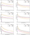 |
Fig. B.1. Predicted number of OBe (left) and normal OB star (right) companions (colour) and different kick scenarios (line style) as a function of mass-transfer efficiency for initially flat binary distributions (top), Sana et al. (2012, middle), and Dunstall et al. (2015, bottom). |
Appendix C: More details of the fiducial model
Appendix C.1: Mass ratios
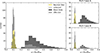 |
Fig. C.1. Predicted mass ratios (MSR/MOB) of massive binary systems after RLO and SN, including systems which became unbound due to the SN (the step size for NSs is 0.01 and for BHs it is 0.05). Left: Total numbers. Right: Case A RLO (top) and B (bottom) separately. |
In Fig. C.1 we show the mass ratio, q = MSR/MOB, of our OB+SR systems. We find values from 0.05 to 0.15 for NS companions and 0.2 to 0.8 for BH companions. As expected, NSs dominate the lower mass ratio regime and BHs the higher mass ratios. BHs whose progenitors evolved through Case A mass transfer reach masses almost as great as their companions star. The distributions for NS can be understood with the values of Fig. 7 and a typical NS mass of 1.3 M⊙. For OB+BH systems this is more complex, as the BH mass is a function of initial stellar mass and the mass of the OB star depends on the accretion efficiency, which is a function of the accretor mass (Eq. (16)). Most features can be derived from Fig. 8.
Appendix C.2: Rotation
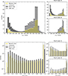 |
Fig. C.2. Same as Fig. 7 but for the equatorial rotational velocity of the OB star (top row) and the ratio of rotational and critical velocity of the OB star (bottom row). Our criterion for an emission-line star is indicated by the dotted line. |
Fig. C.2 shows two different measures for the rotation of the OB star. The upper panel shows the equatorial rotational velocity, vrot, in km/s and the lower panel that relative to the critical velocity, vcr. Form the former we find velocities from 25 up to almost 700 km/s in a bimodal distribution. The first peak is near 50 km/s and the second one is around 550 km/s, which is much broader for BH companions than for NS and unbound systems. Similarly the low vrot/vcr-peak is stronger for BHs than the high velocity peak while for the other two species the high velocity peak is clearly the dominant one. At 350 km/s the velocity distribution has a discontinuity, especially for NS and unbound systems, coinciding with the occurrence of the formation of emission-line stars. This becomes much clearer in the bottom panel. All potential OBe stars lie on the right side of vrot/vcr = 0.95 and form an extremely strong peak. Due to the variance of the critical velocity it was broadened in the upper diagram. The low velocity peak remains broad and also a clear gap between the two modes is present (0.6 to 0.95).
The panels on the right of Fig. C.2 indicate Case A and B. Systems which evolved through Case B only belong to the high velocity peak and are OBe stars. Only a negligible fraction of them has vrot/vcr < 0.95. Thus we can understand this peak as those stars that were spun up by accretion unaffected by tides. The Case A systems are more complex. While one group exists at high velocities, which corresponds to wide Case A evaluations similar to Case B, the low rotational velocity peak is only produced through Case A RLO. It is due to synchronising tides that the peak is so broad as the range of orbital periods after RLO leads to a range of synchronous rotational velocities. BH systems are more strongly affected by this as BHs are more massive and thus induce stronger tides than NSs.
Appendix C.3: Luminosities and temperatures
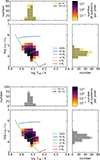 |
Fig. C.3. Predicted HRD positions of OB stars with a NS companions (top) and unbound companions (bottom) in logarithmic colouring together with selected model tracks and the ZAMS. The panels on top and on the right show the temperature and luminosity distributions with predicted emission-line stars highlighted by dotting. |
The HRDs for the companions of NSs (Fig. C.3 top) and those stars which became unbound during the SN (bottom) are very similar as expected. Their luminosities are between 104 L⊙ and 105 L⊙ and their temperatures range from 20 kK to 40 kK which may appear as late O- and early B-type stars. Comparing the population the model tracks, we can see that they lie between the 8 M⊙- and the 20 M⊙-track in agreement with the results of Sect. 5.2.
Appendix C.4: Orbital periods and velocities
Fig. C.4 (top) shows the orbital period. For both BH and NS systems we find orbital periods ranging from 1 d up to 1000 d. Most NS systems have orbital periods of about 30 d while BH systems orbit slightly faster with the mode at 10 d. Both populations’ numbers decrease towards higher periods because of the initial period distribution which prefers close systems and, in case for the NS systems where the accretion efficiency was higher, the reduced stability of mass transfer at greater periods. Main-sequence mass gainers are rapidly spun up during mass transfer. Whether they can appear as OBe stars depends on tidal interaction, which is significant in close binaries. Hence in our synthetic population, normal OB stars dominate the low-period systems. The transition from normal OB to OBe stars occurs around 10 d for NS and 30 d for BH due to difference in masses. As expected, Case A systems tend to show lower and Case B system tend to show larger orbital periods.
The orbital velocity semi-amplitude of the OB star KOB is given by Eq. (17). We show a histogram in Fig. C.4 (bottom). Note that we show the maximally possible semi-amplitude and not the projection onto the celestial sphere, equivalent to an inclination of 90° and with an argument of periastron of 90°. OB stars with NS companions reach velocities up to 100 km/s, but peak at 20 km/s. The companions of BHs show a much broader distribution between 10 km/s and 250 km/s. OB stars in BH systems are typically faster than in NS systems, because of the high BH mass compared to NSs, and are so diverse in velocity semi-amplitude because of the broad mass distribution of BHs. Again, OB stars with a large semi-amplitude tend to be normal OB stars as their orbits are close and tides are braking the stellar rotation. While the distributions for Case A and B look similar for the NS, they clearly differ for the BHs, as the high velocity contribution comes from the Case A systems.
Appendix C.5: Wolf-Rayet stars
We assume, following Shenar et al. (2020), that a HeS with a luminosity above 105.6 L⊙ appears as a WR-star. We show the properties of our simulated O+WR systems in Fig. C.6. As usual we label O-type stars that rotate faster than 95% than their critical rotation as OBe stars, even though the WR or O-type star wind may prevent the formation of a disk or slow the O-type star’s rotation. WR+WR and WR+SR systems are beyond the scope of this work.
The bottom panel shows the luminosities of the two components. While the number of WRs decreases towards higher values as expected from the IMF, the luminosities of the O-type stars are more symmetrical, but still skewed. In the 2D histogram, the population forms a rough triangle since more luminous and thus more massive WRs have more massive and luminous companions. The KOB-KWR diagram (upper left panel of Fig. C.6) shows that the orbital velocity semi-amplitudes correlate tightly. This is not surprising as both stars have mass ratios between 0.5 and 2. Low velocities, especially for the OB stars are somewhat preferred but a notable amount of stars still show values above 200 km/s.
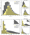 |
Fig. C.4. Same as Fig. 7 but for the orbital period (top row) and orbital velocity semi-amplitude of the OB star (bottom row) |
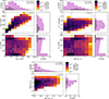 |
Fig. C.6. Predicted properties of WR+O systems with observations of the SMC WR+O systems (Foellmi et al. 2003; Shenar et al. 2016, 2018). Top left: orbital velocity semi-amplitude plane. Middle left: orbital velocity semi-amplitude–rotational velocity plane. Top right: orbital period–mass ratio plane. Middle right: orbital period–rotational velocity plane. Bottom: luminosity-luminosity plane. |
In the two middle panels of Fig. C.6 we investigate the relation between the OB star’s rotational velocity to the orbital properties. We expect orbital periods from 1 d to 1000 d with a preference for short periods around 10 d. Velocity semi-amplitudes range up to 450 km/s, but most common are values of about 100 km/s. As for the OB+BH systems we find a bimodality in the rotation rate of the OB star, but a less pronounced one. The two 2D histograms show again a distribution with two peaks, one for the close systems where tidal braking slowed the OB star down and one for the wide systems where the OB star could keep most of its spin angular momentum.
To compare the synthetic WR+O system to observations, we consider the WR+O binares in the SMC of which four are known (Shenar et al. 2016, 2018). Additionally, there are seven single WR stars. Recently, observations suggest they are truly single (Schootemeijer et al. 2024), which have strong implications on massive binary evolution (Schootemeijer et al. 2024, Paper I) as well as the WR+WR system AB 5 (see however Sect. 3). The WR population in the SMC is thought to be complete (Shenar et al. 2016; Neugent et al. 2018). We use the values given by Shenar et al. (2016) for AB 3, AB 7, and AB 8 and by Shenar et al. (2018) for AB 6.
Fig. C.6 (bottom) shows that AB 6, 7, and 8 have luminosities as predicted, while the OB-luminosity of AB 3 does not match. In the other three panels we find the observations only cover a certain subspace of our simulations. While the orbital periods align with the peak of the simulations (about 10 d), the observations are not distributed as broadly as the models. The same is true for the velocity semi-amplitude distribution (top left panel). We find also a mismatch in the rotational velocities of the OB stars. The observations lie closely together in the brought trough between the two expected maxima (middle panels in Fig. C.6). This mismatch could have a similar origin as for the OB+BH systems, because perhaps the synthetic subpopulation at low rotation velocities corresponds to the observations, but our model overestimates the braking by tides, winds or structural evolution. The top-right panel shows that our synthetic population underestimates the mass of the O-type star compared to the WR star, which indicates that the mass-transfer efficiency might be higher than assumed.
Lastly, we compare our synthetic WR+O systems to Paper I. Both studies reported a similar WR luminosity function; however, differences in the orbital properties did emerge. Our WR velocity semi-amplitude distribution is almost flat, but Paper I prefers low values. Similarly, our period distribution shows a clear maximum while theirs is rather flat even though it has a maximum at low periods. These differences are unexpected since at such high masses we have assumed a low accretion efficiency (10%), relatively close to typical values (5%) of Paper I. However, our model allows for donor stripping at high initial masses for smaller initial mass ratios at low periods than the models of Paper I. Our 30 M⊙ models (online material) results in more low-period WR binaries than their Fig. A.2 (top right). This may explain the lack of WR+O systems with large orbital periods (Schootemeijer et al. 2024).
Appendix D: Discussion: Uncertainties
In this section, we discuss the main uncertainties of our results as well as the alternative model with BH kicks.
Appendix D.1: Stability of mass transfer and mass-transfer efficiency
The key uncertainty of this study is the condition under which a RLO leads to a donor stripping and, in contrast, under which conditions the system mergers. We used the proposition of Schürmann & Langer (2024) to link that to the swelling of the accretor star to the mass-transfer efficiency, which forms the second key uncertainty. Several other conditions have been proposed in the literature. Most prominent is the comparison of the radius evolution of the Roche lobe under mass loss with the adiabatic radius evolution of the donor, most recently investigated by Ge et al. (2010, 2015, 2020a). These studies find a period dependent minimum mass ratio for donor stripping, which itself has a minimum for a 10 M⊙ donor around q = 0.15 and decreases for higher masses. Schürmann & Langer (2024) discussed that their condition is in general more restrictive than the one of Ge et al. (2010, 2015, 2020a). While we assume that donors with a deep convective envelope always result in an unstable mass transfer, aforementioned studies find that mass transfer might be stable for systems close to a mass ratio of unity (see also Quast et al. 2019; Marchant et al. 2021; Ercolino et al. 2024). Finally, Ge et al. (2020b) studied how mass loss from the donor star through its outer Lagrange point could lead to unstable mass transfer and Ge et al. (2024) applied that to HMXBs. They found that non-conservative mass-transfer leads to less stable systems than the conservative case (see their Fig. 7, which can be compared with our Fig. 3), but again our model appears to be more restrictive, as their critical mass-ratio curves always tend to lie within the region where we predict merger by accretor swelling.
An other physically motivated approach was undertaken by Marchant Campos (2018), whose method was also used by Paper I. They stop the deposition of material onto the accretor if it starts to rotate critically. If then the combined luminosity of the two stars is large enough to drive the non-accreted material out of the system, the mass transfer is regarded as stable. The comparison of our Fig. 3 and online material with their Fig. 2, A.1 and A.2 shows drastic differences of the parameter space of mass transfer survivors (see Sect. 6.2 for details). Other studies (e.g. Pols et al. 1991; Hurley et al. 2002; Schneider et al. 2015; Renzo et al. 2019) use fixed minimal mass ratios for stable mass transfer for each Case A and B to decide as the merger criterion, but limit the accretion by the thermal timescale of the accretor, whereby the mass-transfer efficiency becomes a function of period and mass ratio. These mass ratio limits sometimes in tension (e.g. 0.65 for Case A, see de Mink et al. (2007, 2013), Claeys et al. (2014)) and sometimes in agreement (0.25 for Case B, see Schneider et al. (2015), Stevenson et al. (2017)) with our models (see Fig. 3 and Sect. 3).
For this study, we assumed a low mass-transfer efficiency for more massive stars. However according to Fig. 4 also larger values are in agreement with the observed number of WR+O systems within the uncertainties. In Sect. C we found that we under-predict the O-type star mass compared to that of its WR companion, which again suggests mass-transfer efficiencies larger than assumed. In addition to this there are uncertainties in IMF, binary fraction, initial mass ratio and initial orbital period distributions, upper stellar mass limit, size of stable mass-transfer window and recent star-formation rate, which affect the synthetic WR+O population.
Appendix D.2: Case A RLO
Case A mass transfer takes place on the nuclear timescale of the donor and comprises three phases of different structure, which determine the evolution of the stellar masses (Wellstein et al. 2001). The adopted scheme based on the results of Schürmann et al. (2024) might be too simplistic as their underlying models are restricted to a certain set of assumptions of binary physics. Furthermore, we do not resolve the mass-transfer phases in detail but jump after a reasonable amount of time directly to the OB+HeS phase. While we are not interested at the models’ configuration as an Algol system during the mass transfer (e.g. Sen et al. 2022), the detailed evolution may have an imprint on the outcome and the subsequent OB+SR phase, especially at initial mass ratios smaller than about 0.5, where the orbit shirks a lot during RLO (Schürmann et al. 2024).
Appendix D.3: Stellar models
Our predictions rely on the assumed underlying stellar models. A key uncertainty lies in the HeS models. They influence the evolution of our systems firstly through their lifetimes, which determines when an SR forms. This can have an influence on whether a reverse mass transfer occurs. Secondly, their radius evolution determines whether and when a Case BB/BC RLO takes place. This is important as the assumed SMC HeS models are extrapolated from models with solar metallicity (Kruckow et al. 2018) and, most importantly, any thin remaining hydrogen layer was not considered in modelling these stars. As shown by Laplace et al. (2020), the radius evolution of stripped stars has a noticeable effect on the final fate of the system. Furthermore, Ercolino et al. (2024) demonstrated that also a partial removal of the envelope can happen. The occurrence of Case BB/BC mass transfer changes not only the orbital period of the system (Soberman et al. 1997), but also impacts the SN kick (Sect. 2) and determines the final mass of the SR.
Also the calculation of the wind-induced spin-down of our mass gainers bears some uncertainty. Nathaniel et al. (2025) have shown that the numerical treatment of wind angular momentum loss affects the evolution of stellar rotation if stellar winds carry away a significant fraction of the stellar mass. Our approach (Sect. 2.3) leads to a stronger angular momentum loss compared to the scheme used by Paper I, and thus to a somewhat smaller fraction of OBe stars, which spin down during core helium-burning of the stripped star. Although under the assumption of rigid rotation, our approach is more physically correct, it appears not to be favoured when compared to the spin rates of Galactic OB stars (Nathaniel et al. 2025).
Another uncertainty of the stellar models lies in the occurrence of envelope inflation. Sanyal et al. (2015) showed that stellar models heavier than about 40 M⊙ can exceed the local Eddington limit in their envelope, which leads to a large increase in radius and to a convective envelope. As we assume unstable mass transfer for a donor with a deep convective envelope, including this effect into our models could drastically reduce the production of massive HeS by binary stripping and consequently the formation of WR+O and BH+OB systems.
Appendix D.4: Formation of OBe stars
In this study we followed Townsend et al. (2004) and assumed that models with vrot/vcr > 0.95 appear as OBe stars. However, it is not clear whether this is the correct value, nor whether a condition in terms of vrot/vcr would be appropriate overall. Rivinius et al. (2013) summarises that the average vrot/vcr of OBe stars is around 0.854 and the minimum vrot/vcr around 0.77. More recent studies confirmed that OBe stars can rotate substantially sub-critical (Zorec et al. 2016; Balona & Ozuyar 2020; El-Badry et al. 2022; Dufton et al. 2022). On the other hand, interferometric observations of α Eri (Domiciano de Souza et al. 2003, 2012) obtained near-critical rotation.
While fast rotation is likely a necessary criterion for a star to become an OBe star it seems not to be a sufficient condition, as the example of α Leo shows (McAlister et al. 2005). It rotates with vrot/vcr = 0.86 faster than the aforementioned minimum while it is not an OBe star but only of spectral type Bn. Several other condition for a rotating star to become an OBe star such as pulsations and magnetic fields are discussed by Rivinius et al. (2013).
Our simulations yielded that almost all accretors, which rotated faster than vrot/vcr = 0.5 after mass transfer, rotated with at least vrot/vcr = 0.95. Thus the number of OBe stars will change only weakly if we would change our limit from 0.95 (Townsend et al. 2004) to a lower value as 0.77 (Rivinius et al. 2013). A further condition which might need to be fulfilled by a star to become an OBe star may reduce the number of OBe stars in our study. This is problematic as our predicted total number is just about in agreement with the observations (see Sect. 4).
Appendix D.5: BH kick
In Sect. 5, we assumed that the BH receives no birth kick, and thus we find that BH+OB systems do not unbind in our study. In the scenario with flat distribution between 0 km/s and 200 km/s (Fig. 5) we find that their number was reduced by a factor of about two. No consensus about the natal kick has been reached in the literature. Many observational works analysing the position and kinematics of low-mass X-ray binaries argue in favour of a high kick scenario (Podsiadlowski et al. 2002; Gualandris et al. 2005; Willems et al. 2005; Fragos et al. 2009; Repetto et al. 2012; Yanes-Rizo et al. 2025), while others argue for a low kick (Nelemans et al. 1999; Mandel 2016). Repetto & Nelemans (2015) even finds clues for both scenarios depending on the systems. Fryer et al. (2012) and Shao & Li (2014, 2019, 2020, 2021) use for their population syntheses an approach by which the kick of the initially formed NS is reduced by fallback prior to the BH formation. From the detailed modelling site, Janka (2013) is able to explain high BH kicks by an asymmetric SN with fallback. Rahman et al. (2022) on the other hand proposes a mechanism for a low BH kick based on hydrodynamical simulations while Chan et al. (2020) can produce, also with hydrodynamical simulations, both low and high kicks depending on the explosion energy. See Janka et al. (2022) for a recent discussion.
The BH kick does not only affect the total number of OB+BH systems, but also the distributions of orbital parameters such as orbital period and 3D velocity (Tauris & Takens 1998). We reproduced Fig. 6, 8 (lower right), and 13 (top) with a strong BH kick in Fig. D.1. About a third of the BH systems unbinds and we only expect 15 OBe+BH systems and 69 regular OB+BH systems. Especially the systems with OBe stars break apart as they are wider then those with regular OB stars. The eccentricity distribution of the unbound systems is flat (like that of the NS systems, Fig. 12), but avoids values below 0.1. The distribution of orbital periods appears similar to the scenario without kicks, but their number decreases not that much towards larger periods. The combined eccentricity-period distribution is similar to that of the NS systems, but appears to correlate more tightly. The distribution of space velocities with BH kicks also allows for values below 5 km/s. Systems with values above 15 km/s do now contain a emission-line stars. It is quite likely that close OB+BH systems circularise and so the current observations within both eccentricity-period diagrams would allow for both a weak (or no) kick and a large kick at BH formation.
All Tables
All Figures
|
Fig. 1. Schematic evolutionary path from ZAMS to gravitational wave merger, adapted from Kruckow et al. (2018). We focus on the BH + OBe phase. |
| In the text | |
|
Fig. 2. Evolution of the moment of inertia factor of our SMC models. The abscissa is scaled in units of hydrogen burning times. |
| In the text | |
|
Fig. 3. Evolutionary outcome of our binary models with a primary mass of 10 M⊙ at the time when the first SR has formed, or when the system merges, as a function of initial orbital period (Pi) and initial mass ratio (qi) for six different mass-transfer efficiencies (ε). Each black dot represents one model system, and their total number in each plot is 104. We coloured the plane according to the result of the closest model (Voronoi diagram). We mark the boundary between RLO Case A and B by a black line. The occurrence of a later RLO with a HeS donor (i.e. Case BB or BC) is indicated by pink hatches. If the companion to a SR is not a MS star but a post-MS star, we mark it by orange cross-hatches in case it is H-rich (BSG/RSG), or by pink cross-hatches if it is H-poor (HeS). White regions are those with no RLO (top) or RLO at ZAMS (bottom). In grey areas, the outcome is not none of the above (often two SNe immediately after each other due to the final temporal resolution). |
| In the text | |
|
Fig. 4. Predicted number of selected types of stars and binary systems relative to the observed number (given in parentheses in the legend) as a function of mass-transfer efficiency. We show four different assumptions about the stars that become OBe stars – fast rotating accretors (solid line), fast and slow rotating accretors (dashed), fast rotating accretors and merger products (dotted), fast and slow rotating accretors and merger products (dash-dotted) – and three different assumptions about the SN kick – reduced kicks (solid), Hobbs kicks (dashed), and no kicks (dotted). The green line with labelling on the right side of the diagram shows the magnitude of the dimmest synthetic BeXB relative to the dimmest observed one (16.9). The pink shading indicated the uncertainty due to the low number of WR + O systems. The initial binary parameter distributions are flat (top left), according to Sana et al. (2012, bottom left), Sana et al. (2013, bottom right), and Dunstall et al. (2015, top right). |
| In the text | |
|
Fig. 5. Predicted number of OBe star (top) and regular OB star (bottom) companions indicated by colour and different kick scenarios indicated by line style as a function of mass-transfer efficiency for the initial distributions of Sana et al. (2013). |
| In the text | |
|
Fig. 6. Left: Predicted companion fraction of massive (M > 8 M⊙) main-sequence SMC stars in post-mass transfer binaries as function of their mass, including system in which the companion (in general a NS) was unbound during the SN, and excluding merger products. Models that we assumed to appear as emission-line stars are marked with black or white dots (depending on the background colour). Above each mass bin we give the total number of system in that bin. The total number of each companion type is given in the legend distinguishing between emission-line star (first number) and normal OB star (second number). Right: Absolute number of compact companions of OB stars (outer pie chart), and the assumed SN type of the NS progenitor (inner pie chart), predicted by our fiducial SMC population. |
| In the text | |
|
Fig. 7. Predicted masses of the components of massive binary systems after RLO and the formation of a SR. Top row: OB star masses coloured according to their companion type and marked with dots if we expect an emission-line star. The inlays in the upper right corners focus on the upper mass end. Bottom row: BH masses with dots in case of a OBe companion. Note: the vertical axis is logarithmic. Left: Total numbers. Right: Case A RLO (top) and B (bottom) separately. |
| In the text | |
|
Fig. 8. Predicted properties of OB + BH systems. The left panels shows the number of systems in the OB mass–BH mass plane (second row), OB mass–orbital period plane (third row), and OB mass–OB velocity semi-amplitude plane (fourth row) in logarithmic colouring and the other panels are projections of that onto one axis, i.e. the distribution of OB masses (first row left), BH masses (second row right), orbital periods (third row right), and OB star velocity semi-amplitudes (fourth row right), where emission-line stars are marked by white dots. We also show the properties of all dynamically confirmed OB + BH systems in the local group and of the WR + O systems in the SMC with WR masses as BH masses. |
| In the text | |
|
Fig. 9. Predicted HRD positions of OB stars with a BH companions in logarithmic colouring together with selected model tracks and the ZAMS. We include values of all observed OB + BH systems and the O-type star of SMC WR + O systems (see Fig. 8 for the symbols). The panels on top and on the right show the temperature and luminosity distributions with predicted emission-line stars highlighted by dotting. |
| In the text | |
|
Fig. 10. Predicted and observed distribution of V-band magnitudes. The blue bars show the magnitudes of all OB star models (i.e. with HeS, WD, NS, and BH companion and unbound systems) after stable mass transfer. OBe candidates are marked with dots. As observations we show the SMC OBe magnitudes distribution (blue line) from Schootemeijer et al. (2022), the magnitudes of BeXBs (orange line) from Haberl & Sturm (2016)2, SMC X-1 (grey dashed line) and J0045-7319 (brown line). |
| In the text | |
|
Fig. 11. Predicted properties of OB stars that have BH companions with measurements of all dynamically confirmed OB + BH systems in the local group and of the WR + O systems in the SMC. The main panels shows the number of systems in the rotational velocity-velocity semi-amplitude plane (first column, second row), orbital period-velocity semi-amplitude plane (second column, second row), and eccentricity-velocity semi-amplitude plane (second column, third row) in logarithmic colouring and the other panels are projections of that onto one axis, i.e. the distribution of OB rotational velocities (top left), orbital periods (top centre), OB star velocity semi-amplitudes (centre right), and eccentricities (bottom right), where emission-lines stars are marked by white dots. |
| In the text | |
|
Fig. 12. Predicted orbital properties of OB + NS systems with observations of the SMC BeXBs, SMC X-1, and J0045-7319. Centre: Orbital period-eccentricity plane. Top: Orbital period coloured by SN type. Right: Eccentricity coloured by SN type. |
| In the text | |
|
Fig. 13. Predicted space velocities and rotational velocities of OB stars with bound and unbound NS and BH companions with observations of the transverse velocities of isolated SMC OBe stars (blue line and small dots), BeXBs (large blue dots), and SMC X-1 (grey). The median error of the transverse velocities is 23 km/s. Centre: space velocity–rotational velocity plane. Top: space velocities coloured by SN type. The part of the histogram within the grey line indicates the unbound systems. Right: rotational velocities coloured by SN type. |
| In the text | |
|
Fig. B.1. Predicted number of OBe (left) and normal OB star (right) companions (colour) and different kick scenarios (line style) as a function of mass-transfer efficiency for initially flat binary distributions (top), Sana et al. (2012, middle), and Dunstall et al. (2015, bottom). |
| In the text | |
|
Fig. C.1. Predicted mass ratios (MSR/MOB) of massive binary systems after RLO and SN, including systems which became unbound due to the SN (the step size for NSs is 0.01 and for BHs it is 0.05). Left: Total numbers. Right: Case A RLO (top) and B (bottom) separately. |
| In the text | |
|
Fig. C.2. Same as Fig. 7 but for the equatorial rotational velocity of the OB star (top row) and the ratio of rotational and critical velocity of the OB star (bottom row). Our criterion for an emission-line star is indicated by the dotted line. |
| In the text | |
|
Fig. C.3. Predicted HRD positions of OB stars with a NS companions (top) and unbound companions (bottom) in logarithmic colouring together with selected model tracks and the ZAMS. The panels on top and on the right show the temperature and luminosity distributions with predicted emission-line stars highlighted by dotting. |
| In the text | |
|
Fig. C.4. Same as Fig. 7 but for the orbital period (top row) and orbital velocity semi-amplitude of the OB star (bottom row) |
| In the text | |
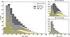 |
Fig. C.5. Same as Fig. 7 but for the space velocity of the OB star. |
| In the text | |
|
Fig. C.6. Predicted properties of WR+O systems with observations of the SMC WR+O systems (Foellmi et al. 2003; Shenar et al. 2016, 2018). Top left: orbital velocity semi-amplitude plane. Middle left: orbital velocity semi-amplitude–rotational velocity plane. Top right: orbital period–mass ratio plane. Middle right: orbital period–rotational velocity plane. Bottom: luminosity-luminosity plane. |
| In the text | |
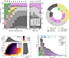 |
Fig. D.1. Same as Fig. 6, 11 (lower right), and 13 (top), but with a BH kick. |
| In the text | |
Current usage metrics show cumulative count of Article Views (full-text article views including HTML views, PDF and ePub downloads, according to the available data) and Abstracts Views on Vision4Press platform.
Data correspond to usage on the plateform after 2015. The current usage metrics is available 48-96 hours after online publication and is updated daily on week days.
Initial download of the metrics may take a while.