© The Authors 2025

1. Introduction

Binaries are common in nature, with some estimates of stellar multiplicity being close to unity based on modern astrometric surveys (Duchêne & Kraus 2013; El-Badry 2024). Tidal forces play an important role in the rotational and orbital evolution of close systems, such as binary stars (e.g., Zahn 2013; Barker 2022, and references therein), exoplanetary hot-Jupiter systems (e.g., Jackson et al. 2008; Bolmont & Mathis 2016; Lazovik et al. 2024), planet-satellite systems (Counselman 1973; Fuller et al. 2024, for a review), and merging neutron stars (NSs; Damour & Nagar 2009; Taniguchi & Shibata 2010). Their impact can generally be quantified in terms of two components, these being the equilibrium and dynamical tides. The former exists even in the zero-frequency limit and describes bulk geometric large-scale deformations, while the latter relates to the excitation of internal (damped) waves (e.g., Ogilvie 2014; Hinderer et al. 2016; Andersson & Pnigouras 2020).

A perturbative and often even linear treatment of tides provides an excellent approximation in many astrophysical systems of interest. There are cases, however, where the validity of a linear approximation is less certain (see Sect. 4 of Ogilvie 2014, for a review). One such scenario – central to this paper – involves resonances in NS mergers. As the binary shrinks due to gravitational-wave (GW) radiation-reaction, the orbital frequency “chirps” upward toward coalescence (e.g., Peters 1964). When the tidal driving frequency approaches the oscillation frequency of a mode inside one of the stars, that mode’s amplitude grows rapidly. The amplitude may peak at a value that depends on the degree of orthogonality between its eigenfunction and the appropriate multipole component of the tidal field (“overlap”; Press & Teukolsky 1977; Alexander 1987), or if the resonance window lags behind the ever-increasing tidal forcing frequency, at a value that depends on how rapidly the frequency evolves away from the resonant frequency. For some mode classes, the amplitude could theoretically grow beyond the linear regime, necessitating nonlinear corrections (e.g., Yu et al. 2023; Kwon et al. 2024, 2025) or tidal nonlinearities (Pitre & Poisson 2025) to be taken into account to more accurately assess how tides affect GW or electromagnetic observables.

Numerical relativity simulations have highlighted the impact of nonlinearities on GW dephasing for the fundamental (f-) mode (Kuan et al. 2025). Though subdominant, gravity (g-) modes – supported by internal composition and/or entropy gradients – may also non-negligibly accelerate inspiral in mergers as their eigenfrequencies are sufficiently low (∼10² Hz) to be excited approximately a few seconds prior to coalescence while maintaining sizeable overlaps (Kokkotas & Schafer 1995; Kuan et al. 2021a; Passamonti et al. 2021; Hegade 2024). Since these modes offer valuable microphysical information and it is hoped that templates will be matched to GW data in the future, it is important that their nonlinear saturation be quantified. For stars retaining a high angular frequency into old age (Ω ≳ 10² Hz; “recycled pulsars”) the inertial class of modes (restored by Coriolis acceleration) may also be relevant (Lai & Wu 2006; Suvorov & Kokkotas 2020). With both buoyancy and rotation present, the two branches merge to some degree and go under a “gravito-inertial” label (see, e.g., Aerts & Tkachenko 2024). Here we present a method for modeling the nonlinear saturation of such hybrid modes. In particular, nonlinearities are treated at the level of the magnetohydrodynamic (MHD) equations of motion, rather than via secondary couplings between linear modes as studied previously (e.g., Weinberg et al. 2013; Pnigouras & Kokkotas 2015; Zhou & Zhang 2017). This marks the first time, therefore, that this class and their saturation have been modeled consistently at a nonlinear level for rotating, tidally forced NSs.

Nonlinear, tidally forced inertial modes have been studied in numerical simulations modeling convective envelopes of giant gaseous planets and low-mass stars in close binary systems (Favier et al. 2014; Barker 2016; Astoul & Barker 2022). Due to the generation of differential rotation, transfer rates of tidal energy (i.e., tidal dissipation) can be either higher or lower by up to ∼3 orders of magnitude relative to linear-theory predictions at some frequencies (especially for thin shells, large tidal amplitudes, and low viscosities; Astoul & Barker 2023). In radiative regions, differential rotation can also arise from the deposition of gravity wave angular momentum at corotation resonances – when the horizontal velocity of the wave matches the local speed of the fluid – as predicted by Goldreich & Nicholson (1989) in the envelopes of early-type stars. This result has been confirmed for the radiative cores of solar-like stars in 2D and 3D spherical nonlinear simulations, where the core is progressively spun up from inside out by tidal gravity wave breaking (or weakly nonlinear damping) near the center of the star (Barker & Ogilvie 2010; Barker 2011; Guo et al. 2023). Here, we also study such nonlinear effects but in the context of gravito-inertial modes in NSs by building on the formulation used in Astoul & Barker (2022) to split tides into equilibrium and dynamical components while adding buoyancy and thermal diffusion.

Based on this “split formulation”, accounting for the fact that the Brunt-Väisälä (BV) frequency of a cold NS is typically much lower than its dynamical (hydrostatic) response frequency, we ignored surface waves and assumed impermeable and stress-free boundaries. We used the pseudo-spectral MagIC¹ code (Wicht 2002; Gastine & Wicht 2012; Schaeffer 2013) to solve the hydrodynamical equations in a spherical shell under the Boussinesq approximation (Spiegel & Veronis 1960). The equations were coupled to the leading-order (ℓ = m = 2) tidal potential for frequencies relevant to the late-stages of inspiral, with (effective) viscosity included in anticipation of damping and turbulence. Magnetic effects may be especially relevant in some mergers, as there is evidence to suggest that those systems, which release nonthermal gamma-ray burst (GRB) precursor flares (≲5% of mergers; Wang et al. 2020; Coppin et al. 2020), contain magnetars with near-surface fields of B ≳ 10¹³ G (e.g., Xiao et al. 2024). Fields of this strength can influence mode spectra (e.g., Suvorov et al. 2022; Kuan et al. 2021a) or merger dynamics directly (e.g., Ciolfi 2020). A thorough comparison with a linear scheme, using the Dedalus3 code (Burns et al. 2020), is also provided to explore the direct impact of nonlinearities.

Although this is primarily a “methods” paper where the above-described strategy is presented in detail and then integrated numerically for a variety of setups, we also explore some astrophysical applications. For example, incorporating magnetic fields naturally allows for the investigation of dynamo action, namely the magnetorotational instability (MRI; Balbus & Hawley 1998; Astoul & Barker 2025), sourced by the differential rotation induced by non-axisymmetric mode activity. The nonlinear scheme allows, in principle, for us to compare with the idea suggested by Suvorov et al. (2024a) that magnetar-level fields are generated on the verge of coalescence rather than preserved over cosmological timescales. As such, longevity appears difficult to reconcile with magnetothermal evolutions (Pons & Viganò 2019).

This paper is organized as follows: Section 2 introduces the neutron-star hybrid modes and the equations governing both the linear (Sect. 2.2.1) and new nonlinear (Sect. 2.2.2) schemes used throughout, with details on numerical implementation provided in Sect. 2.4. Results for both g- and more general gravito-inertial modes in cases with rotation are given in Sect. 3 for the linear and Sect. 4 for the nonlinear cases, respectively. Astrophysical implications are briefly explored in Sect. 5, with discussion provided in Sect. 6. Key results are summarized in Sect. 7.

2. Modeling of the tidal resonance of gravito-inertial modes in a neutron star binary

2.1. Simplified neutron star model

In this work, we studied the tidal forcing of gravito-inertial modes in the late stages of a binary neutron-star inspiral. To do this, we used methods and formulations from the stellar and planetary community, where linear codes and, more recently, nonlinear simulations are developed following the split methodology mentioned earlier. As a first study in the context of binary NSs, we adopted the idealized Boussinesq approximation that allows us to study the impact of stable entropy and/or composition stratification while keeping the simulations computationally efficient so that the parameter space can be efficiently explored. This approximation corresponds to assuming that variations in mass density can be neglected except as they contribute to buoyancy, i.e., the fluid is otherwise incompressible and sound waves are filtered (Spiegel & Veronis 1960). This approximation is partly justified because the velocities of resonant modes are strictly subsonic, as found in previous studies (Kuan et al. 2021a; Passamonti et al. 2021; Suvorov et al. 2024a), while the constant density assumption is made for simplification (see Sect. 6.2). We used the Newtonian Navier-Stokes equations throughout and neglected the effects of general relativity, as the Boussinesq approximation is already a more restrictive approximation. Note that we also assumed the neutron-star interior to contain only a normal fluid, ignoring superfluidity and superconductivity.

The fluid stratification is characterized by the background BV frequency,

$$\begin{array}{c}\hfill N^2\equiv -\frac{g}{{\rho }_0}({\frac{\partial \rho }{\partial S}|}_{P,Y_e}\frac{\mathit{dS}}{\mathit{dr}}+{\frac{\partial \rho }{\partial Y_e}|}_{P,S}\frac{d{Y}_e}{\mathit{dr}}),\end{array}$$(1)

where g,  ρ₀,  ρ, S,  P and Y_e are background quantities, respectively, the gravitational acceleration, background uniform density (see below), density, entropy, pressure, and electron fraction. As a simplification, we assumed that the BV frequency depends only on one dimensionless background buoyancy variable, chosen here as $\stackrel{\sim }{b}=-\frac{\rho }{{\rho }_0}$. In our model, we assumed that the background density and BV frequency stay constant in time. The latter condition amounts to assuming that (nuclear) weak interaction timescales are much longer than internal hydrodynamical timescales and that the entropy entrained by fluid motions is negligible. As a result, the background flow is adiabatic and the frozen compositional gradient gives rise to buoyancy. We evolved density perturbations through the buoyancy variable $b=-\frac{\delta \rho }{{\rho }_0}$, where δρ is the perturbed density. In this work, we refer to the diffusion process associated with this buoyancy variable as the thermal diffusivity, κ_th. This does not reduce the (numerical) generality of the problem as the buoyancy variable could be entropy or composition and would play exactly the same role in either case (ignoring double-diffusive effects). We used an explicit dissipation and nonadiabatic processes for the perturbations for numerical stability reasons, as the numerical dissipation is not enough to stabilize the simulation with (pseudo-)spectral methods. For dissipation processes, we adopted uniform profiles of viscosity ν and thermal κ_th (or compositional κ_comp) diffusivities with ν = κ_th for the sake of simplicity².

The model for the NS used is that of a spherical shell with a uniform density ρ₀. This quantity is determined by the mass of the primary, given as $M_1=\frac{4}{3}\pi {\rho }_0{R}_o^3$, where R_o is the stellar radius of the primary and depends on the equation of state (EOS). For tests of the new formulation, we first assumed that the shell has an inner radius R_i, whose ratio to the stellar radius (R_o) is set as α ≡ R_i/R_o = 0.5. This value has been used in previous studies of (gravito-)inertial waves in planets and stars as a standard (e.g., Ogilvie 2009; Favier et al. 2014; Astoul & Barker 2022; Pontin et al. 2023) and it reduces the numerical costs as a lower resolution can be taken. However, a thin shell with α = 0.5 is a bad approximation for NSs as changing the size of the shell also changes the resonant frequencies and the mode amplitudes. Therefore, for astrophysical applications to NSs, we instead took α = 0.1 to approximate a whole NS without substantially increasing numerical costs. In addition, g-mode eigenfunctions in NSs peak away from the region $\frac{R}{R_o}<\alpha$ (Kuan et al. 2021a) so this approximation is reasonable (see Sect. 5.1 for a direct comparison of the linear modes).

2.2. Governing equations

We placed ourselves in a frame rotating with the star and assumed an initial hydrostatic balance, i.e., ${\rho }_{0}g=-\frac{d\stackrel{\sim }{P}}{\mathit{dr}}$ where g is the gravitational acceleration and $\stackrel{\sim }{P}$ is the background pressure. The equations for the perturbed velocity components can then be written as

$$\begin{array}{cc}\hfill \mathbf{\nabla }·\mathit{u}& =0,\hfill \end{array}$$(2)

$$\begin{array}{cc}\hfill \frac{\partial \mathit{u}}{\partial t}+(\mathit{u}·\mathbf{\nabla })\mathit{u}& =-\frac{\mathbf{\nabla }p}{{\rho }_0}-2{\mathbf{\Omega }}_{\mathit{s}}\times \mathit{u}-b\mathit{g}-\mathbf{\nabla }\mathbf{\Psi }+\mathbf{\nabla }·{\mathit{\tau }}_{\nu },\hfill \end{array}$$(3)

where u,  p and b are velocity, pressure, and buoyancy perturbations, Ω_s is the (constant) stellar angular frequency of the background star, Ψ is the tidal potential, and τ_ν is the viscous stress tensor. Note that the components of velocity are designated by u_i with spherical polar components i ∈ [r, θ, ϕ] instead of the contravariant equivalent uⁱ in GR calculations. Centrifugal and other forces that may lead to a nonspherical cavity are neglected. We chose to neglect perturbations in the gravitational potential for the sake of simplicity and because they are not expected to play a significant role in the context of our Boussinesq system (Ogilvie & Lin 2004, though for quantitative predictions of resonances they may need to be included). This hypothesis is discussed in detail in Sect. 6.4. This makes it easier to compare between formulations as we neglected the contributions of the gravitational potential perturbations due to the equilibrium tides characterized by the Love number k₂ (see Sect. 6.4).

In our Boussinesq model, the heat equation thus takes the form

$$\begin{array}{c}\hfill \frac{\partial b}{\partial t}+(\mathit{u}·\mathbf{\nabla })b+u_r\frac{d\stackrel{\sim }{b}}{\mathit{dr}}={\kappa }_{\mathrm{th}}{\mathbf{\nabla }}^{2}b,\end{array}$$(4)

where the global gradient of the buoyancy variable $\frac{d\stackrel{\sim }{b}}{\mathit{dr}}$ is linked to the radially dependent BV frequency through

$$\begin{array}{c}\hfill N^2=-\frac{g}{{\rho }_0}\frac{d\stackrel{\sim }{b}}{\mathit{dr}}·\end{array}$$(5)

In the case of pure entropy or composition stratification, we would obtain $\frac{d\stackrel{\sim }{b}}{\mathit{dr}}={\frac{\partial \rho }{\partial S}|}_{P,Y_e}\frac{\mathit{dS}}{\mathit{dr}}$ or $\frac{d\stackrel{\sim }{b}}{\mathit{dr}}={\frac{\partial \rho }{\partial Y_e}|}_{P,S}\frac{d{Y}_e}{\mathit{dr}}$, respectively.

Leaving aside events involving dynamical capture, orbital eccentricity is expected to be erased long before coalescence in a neutron-star binary merger (e.g., Peters 1964). Because of this and for simplicity, we considered a circular but asynchronous orbit with no spin-orbit misalignment (though cf. Kuan et al. 2023). The dominant (quadrupolar) component of the tidal potential can be written as (e.g., Zahn 1966)

$$\begin{array}{c}\hfill \mathrm{\Psi }={\mathrm{\Psi }}_0{r}^2{Y}_2^2(\theta ,\varphi )e^{-i\widehat{\omega }t},\end{array}$$(6)

where Y_l^m is a spherical harmonic of degree ℓ and order m, and the strength of the potential is (see, for instance, Eq. (3) and Table 1 in Ogilvie 2014)

$$\begin{array}{c}\hfill {\mathrm{\Psi }}_0=\sqrt{\frac{6\pi }{5}}\frac{M_2}{M_1}{\omega }_d^2{\left(\frac{R_o}{a}\right)}^3,\end{array}$$(7)

where M₂ is the companion mass, a is the orbital semimajor axis, and ${\omega }_d=\sqrt{G{M}_1/R_o^3}$ is the dynamical frequency with G being the gravitational constant. In the rotating frame introduced earlier, the tidal forcing frequency reads $\widehat{\omega }=2({\mathrm{\Omega }}_o-{\mathrm{\Omega }}_s)$, where Ω_o is the orbital frequency, and we note that $\widehat{\omega }$ can be negative. Equations (2)–(4) constitute the full nonlinear equations considered here. The reader who is less interested in details and tests regarding the new formulation and numerical implementations may skip ahead to Sect. 4 for discussions on nonlinear saturation amplitudes or Sect. 5 for the astrophysical application of binary NSs mergers.

2.2.1. Linear equations

To have a point of comparison with previous literature, we first derived the equations describing linear gravito-inertial modes. These are similar to those from Pontin et al. (2024), which read

$$\begin{array}{cc}\hfill \mathbf{\nabla }·\mathit{u}& =0,\hfill \end{array}$$(8)

$$\begin{array}{cc}\hfill \frac{\partial \mathit{u}}{\partial t}& =-\frac{\mathbf{\nabla }p}{{\rho }_0}-2{\mathbf{\Omega }}_{\mathit{s}}\times \mathit{u}-b\mathit{g}-\mathbf{\nabla }\mathbf{\Psi }+\nu {\mathbf{\nabla }}^2\mathit{u},\hfill \end{array}$$(9)

$$\begin{array}{cc}\hfill \frac{\partial b}{\partial t}+u_r\frac{d\stackrel{\sim }{b}}{\mathit{dr}}& ={\kappa }_{\mathrm{th}}{\mathrm{\nabla }}^{2}b.\hfill \end{array}$$(10)

In this study, we considered three distinct BV profiles: a uniform BV frequency in Sect. 3, a uniform buoyancy variable gradient, which leads to a BV frequency varying radially and linearly with the gravitational acceleration of a homogeneous body, g = −ge_r = −g₀re_r in Sect. 4, and a realistic profile from Suvorov et al. (2024a) in Sect. 5. To solve the linear system, we took a non-penetrating boundary condition for the radial velocity at the inner boundary and a free surface where normal stress vanishes at the outer boundary following Pontin et al. (2023, 2024). We further imposed stress-free conditions (no tangential stress) at the two boundaries, with either the buoyancy variable fixed (b = 0) or its gradient $(\frac{\partial b}{\partial r}=0)$ at the two boundaries, since this has little impact on the resonances (Pontin et al. 2023). This setup will be referred to as a “full formulation” hereafter as it encompasses both the equilibrium and dynamical tides. However, the implementation of a free surface in a fully nonlinear code is prohibitively costly, as surface oscillations would occur at frequencies of ∼ω_d, while the rotation rate and (gravito-inertial or BV frequency) mode frequencies are much lower for NSs.

2.2.2. A new formulation to excite gravito-inertial modes

A derivation for separating equilibrium and dynamical tides, especially for inertial modes, can be found in numerous studies (see, for example, Ogilvie & Lin 2004; Zahn 2013; Ogilvie 2013; Astoul & Barker 2022, and references therein). For the treatment of the gravito-inertial modes, we took a slightly different approach to the one used in Dhouib et al. (2024): as the equilibrium tide corresponds to the instantaneous hydrostatic response to the tidal force, we assumed that reequilibration between pressure and gravity is reached instantaneously compared to the buoyancy variables (i.e., p and g evolve much faster than b in the current context). Another way of describing this treatment is to assume that the advection of the background gradient of the buoyancy variables by the equilibrium tide is part of the heat equation, Eq. (4), for the dynamical tides. It acts as an effective (“heating” or buoyancy driving) forcing of the waves by the equilibrium tide (see Eq. (16)). Then the heat equation for the equilibrium buoyancy variable (i.e., b_e) would be

$$\begin{array}{c}\hfill \frac{\partial b_e}{\partial t}={\kappa }_{\mathrm{th}}{\mathbf{\nabla }}^2{b}_e,\end{array}$$(11)

which gives b_e = 0 as there are no source terms. This corresponds to assuming that the equilibrium tide flow u_e is fully incompressible, and thus we adopted the expression valid for ℓ = m = 2 inertial modes (Ogilvie 2013; Lin & Ogilvie 2018; Astoul & Barker 2022, 2023)

$$\begin{array}{c}\hfill {\mathit{u}}_{\mathit{e}}=\text{Re}[i\widehat{\omega }\mathbf{\nabla }X{e}^{-i\widehat{\omega }t}],\end{array}$$(12)

with

$$\begin{array}{c}\hfill X(r,\theta ,\varphi )=\frac{C_t}{2(1-{\alpha }^5)}[r^2+\frac{2}{3}{\alpha }^5{r}^{-3}]Y_2^2(\theta ,\varphi ),\end{array}$$(13)

where u is satisfying the free-surface boundary condition at the top and impenetrability at the bottom. Here C_t = (1+Re[k₂²])ϵ is the tidal force amplitude related to the real part of the quadrupolar Love number Re[k₂²] and the tidal amplitude parameter ϵ = (M₂/M₁)(R_o/a)³.

Equation (12) leads to a static pressure perturbation p_e that, in addition to u_e, compensates the tidal force in the Navier-Stokes equations. With this equilibrium tide, the linear equations for the leftover velocity u′ = u − u_e, pressure p′ = p − p_e and b′ = b − b_e become

$$\begin{array}{cc}\hfill \mathbf{\nabla }·\mathit{u}\mathbf{\prime }& =0,\hfill \end{array}$$(14)

$$\begin{array}{cc}\hfill \frac{\partial \mathit{u}\mathbf{\prime }}{\partial t}& =-\frac{\mathbf{\nabla }p\prime }{{\rho }_0}-2{\mathbf{\Omega }}_{\mathit{s}}\times \mathit{u}\mathbf{\prime }-2{\mathbf{\Omega }}_{\mathit{s}}\times {\mathit{u}}_{\mathit{e}}-b\prime \mathit{g}+\nu {\mathbf{\nabla }}^{2}u\prime ,\hfill \end{array}$$(15)

$$\begin{array}{cc}\hfill \frac{\partial b\prime }{\partial t}+u_r^{\prime }\frac{d\stackrel{\sim }{b}}{\mathit{dr}}& =-u_{e,r}\frac{d\stackrel{\sim }{b}}{\mathit{dr}}+{\kappa }_{\mathrm{th}}{\mathbf{\nabla }}^{2}b\prime .\hfill \end{array}$$(16)

This system has two effective tidal forcing: f_t = −2Ω_s × u_e, the Coriolis acceleration on the equilibrium tidal flow u_e in the momentum equation, and $f_N=-{\mathit{u}}_{\mathit{e}}·\mathbf{\nabla }\stackrel{\sim }{b}$, the advection of the background entropy gradient by the equilibrium tide in the heat equation. This second term allows us to excite g-modes even in a nonrotating case. It is usually not included in more general split formulations, where background density is not uniform (Ogilvie & Lin 2004; Dhouib et al. 2024), as it is considered as part of an equilibrium tidal buoyancy variable (i.e., entropy/temperature) term. This approach may lead to issues for g-modes in an uniform density star that may not be present with a nonuniform density, depending on the definition of the equilibrium tide. Indeed, in the Boussinesq approximation, we consider that density perturbations are only due to entropy and/or composition perturbations but, as described by Ogilvie (2013), such a density perturbation corresponds to a delta spike at the surface with radial displacement. The heat equation would then force the radial displacement to be zero, yielding a contradiction. Our formalism is a workaround to avoid this issue. A comparison between formalisms with a nonuniform density ρ₀ is planned for a future study. The use of a fixed surface also means we cannot have surface modes and, therefore, our formalism is valid for Ω_s², N² ≪ ω_d², which is the case for NSs and some gas giants (Dewberry 2023; Lin 2023; Suvorov et al. 2024a).

In the following, we omit primes when using the above-introduced formulation, hereafter called the “split formulation”, where the nonlinear equations read

$$\begin{array}{cc}\hfill \mathbf{\nabla }·\mathit{u}& =0,\hfill \end{array}$$(17)

$$\begin{array}{cc}\hfill \frac{\partial \mathit{u}}{\partial t}+(\mathit{u}·\mathbf{\nabla })\mathit{u}& =-\frac{\mathbf{\nabla }p}{{\rho }_0}-2{\mathbf{\Omega }}_{\mathit{s}}\times \mathit{u}+{\mathit{f}}_{\mathit{t}}-b\mathit{g}+\mathbf{\nabla }·{\mathit{\tau }}_{\nu },\hfill \end{array}$$(18)

$$\begin{array}{cc}\hfill \frac{\partial b}{\partial t}+(\mathit{u}·\mathbf{\nabla })b+u_r\frac{d\stackrel{\sim }{b}}{\mathit{dr}}& =-u_{e,r}\frac{d\stackrel{\sim }{b}}{\mathit{dr}}+{\kappa }_{\mathrm{th}}{\mathbf{\nabla }}^{2}b.\hfill \end{array}$$(19)

With this split formulation, we used non-penetrating boundary conditions for the velocity at both outer and inner boundaries. We also kept the stress-free boundary conditions as in the previous formulations. For both formulations, we tested that the buoyancy variable boundary conditions did not impact significantly the results and chose, therefore, the one that gave the strongest mode amplitudes, setting the gradient of the buoyancy variable to zero, i.e., $\frac{\mathit{db}}{\mathit{dr}}=0$.

2.2.3. Energy equations

As we have a new forcing term in the equations, we focus on deriving the new energy balance to understand the dissipation and saturation of tidally forced modes. The dissipation terms correspond to the volume integrated viscous D_ν and thermal D_κ dissipation rates given by

$$\begin{array}{c}\hfill D_{\nu }=-{\displaystyle {\int }_V}{\rho }_0\nu \mathit{u}·{\mathbf{\nabla }}^2\mathit{u}\mathrm{d}V,D_{\kappa }=-{\displaystyle {\int }_V}{\rho }_0{\kappa }_{\mathrm{th}}\frac{g^2}{N^2}b{\mathbf{\nabla }}^{2}b\mathrm{d}V.\end{array}$$(20)

By the standard definition of work, the power injected by the tidal force in the full formulation is

$$\begin{array}{c}\hfill P_{\mathrm{\Psi }}={\displaystyle {\int }_V}{\rho }_0\mathit{u}·(-\mathbf{\nabla }\mathrm{\Psi })\mathrm{d}V.\end{array}$$(21)

In this formulation, the energy balance has already been derived by Pontin et al. (2023, 2024) and is given by

$$\begin{array}{c}\hfill P_{\mathrm{\Psi }}=\frac{d{E}_K}{\mathit{dt}}+\frac{d{E}_{\mathit{PE}}}{\mathit{dt}}+D_{\nu }+D_{\kappa },\end{array}$$(22)

where E_K and E_PE are respectively the kinetic and potential energy of the star. Their respective rates of change are

$$\begin{array}{c}\hfill \frac{d{E}_K}{\mathit{dt}}={\displaystyle {\int }_V}\frac{{\rho }_0}{2}\frac{{\partial |u|}^2}{\partial t}dV,\frac{d{E}_{\mathit{PE}}}{\mathit{dt}}={\displaystyle {\int }_V}\frac{g^2}{2N^2}\frac{\partial b^2}{\partial t}dV,\end{array}$$(23)

except for N² = 0 where one has $\frac{d{E}_{\mathit{PE}}}{\mathit{dt}}=0$. At saturation and averaged over a forcing period of $2\pi /\widehat{\omega }$, energy conservation implies

$$\begin{array}{c}\hfill P_{\mathrm{\Psi }}=D_{\nu }+D_{\kappa }.\end{array}$$(24)

For the split formulation, the power injected by the effective body force f_t due to Coriolis force of the equilibrium tide is given by

$$\begin{array}{c}\hfill P_{\mathrm{Cor}}={\displaystyle {\int }_V}{\rho }_0\mathit{u}·{\mathit{f}}_{\mathit{t}}\mathrm{d}V.\end{array}$$(25)

To obtain the power for the effective forcing f_N in the heat equation, it is easier to use the buoyancy power in the Navier-Stokes equation that is defined by

$$\begin{array}{c}\hfill P_{\mathrm{buoy}}=-{\displaystyle {\int }_V}{\rho }_0{u}_{r}bg\mathrm{d}V.\end{array}$$(26)

By substituting u_r using the heat equation, we obtain the buoyancy power due to the tidal entropy forcing

$$\begin{array}{c}\hfill P_{\mathrm{buoy},e}={\displaystyle {\int }_V}{\rho }_0{u}_{e,r}bg\mathrm{d}V.\end{array}$$(27)

This gives the global balance of energy in the split formulation

$$\begin{array}{c}\hfill P_{\mathrm{Cor}}+P_{\mathrm{buoy},e}=D_{\nu }+D_{\kappa }.\end{array}$$(28)

Note that this final balance is obtained by substituting the buoyancy power, P_buoy, by its saturation balance in the heat equation, P_buoy = P_buoy, e − D_κ, which accounts for the impact of thermal dissipation on the available power for the tidal flows.

2.3. Parameter space corresponding to resonant g-modes for a neutron star binary

Previous linear studies have shown that g-modes could be resonantly excited in a NS binary. We build on the study by Suvorov et al. (2024a) for our NS models constructed with the APR4 EOS (Akmal et al. 1998) coupled to a Douchin and Haensel (DH) crust (Douchin & Haensel 2001). For our tests of both linear (Sect. 3) and nonlinear calculations (Sect. 4), we studied the resonance of g-modes in a 2.0 M_⊙ NS, where the frequency of the first g-mode is N = 102.89 Hz. We also considered an equal mass binary, so that the characteristic frequency is ω_d = 2288 Hz for both stars. We varied the rotation rate Ω_s and rate Ω_s = 2πΩ_s in this study with ${\mathrm{\Omega }}_s=\frac{100}{\pi }$ Hz being a “standard” value. The resonant gravity, inertial, or mixed gravito-inertial modes are well-separated from ω_d and lie in the low-frequency regime. It should be noted that we express frequencies throughout in units of Hz: the reader should be aware, however, that many of these are angular frequencies (e.g., the spin frequency Ω_s) and thus are 2 π times the value of the frequency in these units. In addition, the tidal amplitude is as small as ϵ ∼ 10⁻³ near the g-mode resonance when 2Ω_o ∼ N. According to previous studies on inertial modes (Astoul & Barker 2022, 2023), this places us firmly in the linear regime but this could change for a lower viscosity, higher aspect ratio (α > 0.5), or for the resonant gravito-inertial modes with the highest kinetic energy.

With respect to dissipation, we chose our standard viscosity and thermal diffusivity to be ν = κ = 10⁻⁶R_o²ω_d ≈ 1.7 × 10¹⁰ cm² s⁻¹, similar to Pontin et al. (2023, 2024). This value is many orders of magnitude higher than the microphysical viscosity expected in NSs (Thompson & Duncan 1993) but is chosen to prevent numerical issues. These choices give an Ekman number of

$$\begin{array}{c}\hfill Ek\equiv \frac{\nu }{R_o^2{\mathrm{\Omega }}_s}\approx 7.2\times {10}^{-5}.\end{array}$$(29)

The control parameter for the BV frequency in the simulations is the Rayleigh number, defined as

$$\begin{array}{c}\hfill Ra\equiv -\frac{N^2{R}_o^4}{\kappa \nu }\approx -2.02\times {10}^9.\end{array}$$(30)

As an astrophysical application, we study a more standard equal-mass NS binary of 1.6 M_⊙ in Sect. 5. The characteristic frequency is then ω_d = 1941 Hz. We also used a “realistic” BV frequency and its value at the outer boundary to define the Rayleigh number. The dimensionless numbers are Ra = −5.1 × 10¹⁰ and Ek = 6.2 × 10⁻⁵ − 1.99 × 10⁻⁵ with rotation rates of ${\mathrm{\Omega }}_s=\frac{100}{\pi }-100$ Hz, respectively.

2.4. Numerical methods

To solve the linear equations, we used the spectral MHD code Dedalus3 (Burns et al. 2020). Dedalus has been used to handle different types of hydrodynamical and MHD problems, including convection, waves, and magnetic fields in an unstratified or stratified medium in many studies (Lecoanet et al. 2017; Couston et al. 2018; Ji et al. 2023). Using the full formulation, we benchmarked the code results against the study by Pontin et al. (2023) and are therefore confident in the results for when using the split formulation. The number of grid points used for the linear problem was (n_r, n_θ) = (200 − 400, 200 − 400) depending on the parameters.

In order to integrate the nonlinear equations in time, Eqs. (17)–(19), we used the benchmarked pseudo-spectral code MagIC (Wicht 2002; Gastine & Wicht 2012; Schaeffer 2013). MagIC solves the 3D MHD equations in a spherical shell using a poloidal-toroidal decomposition for the velocity and the magnetic field (made possible by the solenoidal assumption on u),

$$\begin{array}{cc}\hfill {\rho }_0\mathit{u}& =\mathbf{\nabla }\times \mathbf{\nabla }\times \left(W{\mathit{e}}_{\mathit{r}}\right)+\mathbf{\nabla }\times \left(Z{\mathit{e}}_{\mathit{r}}\right),\hfill \end{array}$$(31)

$$\begin{array}{cc}\hfill \mathit{B}& =\mathbf{\nabla }\times \mathbf{\nabla }\times \left(b{\mathit{e}}_{\mathit{r}}\right)+\mathbf{\nabla }\times \left(a_j{\mathit{e}}_{\mathit{r}}\right),\hfill \end{array}$$(32)

where W and Z are the poloidal and toroidal kinetic scalar potentials, respectively, while b and a_j are the magnetic potentials. The scalar potentials and the pressure P are decomposed on spherical harmonics for the colatitude (θ) and the azimuthal (ϕ) angles, together with Chebyshev polynomials in the radial direction. For more detailed descriptions of the associated spectral transforms and the numerical method, we refer to Gilman & Glatzmaier (1981), Tilgner & Busse (1997), and Christensen & Wicht (2015).

The nonlinear simulations presented in this paper were performed using a standard grid resolution of (n_r, n_θ, n_ϕ) = (257, 256, 512). Some of the simulations have a cutoff m_max in the spherical harmonics to speed up the simulations; for simulations in Sect. 4, m_max = 85 is enough to ensure convergence as the dominant mode corresponds to m = 2. The code uses an adaptive timestep where we added a maximum value of $d{t}_{\max }=1/(10\widehat{\omega })$ to ensure the resolution of the forced frequency.

3. Linear tests of the formulation

In this section we discuss how we tested the new split formulation. As a first step, we demonstrate how we successfully reproduced the properties of g-modes obtained with the “full” formulation (Sect. 3.1). This set us up for studying gravito-inertial modes to check whether the two effective tidal forcings give the correct geometry (i.e., structure) and amplitude of the gravito-inertial modes (Sect. 3.2). In order to compare more easily with Pontin et al. (2023), we adopt in this section the same units as that study: R_o = 1, ω_d = 1 and ρ₀ = 1.

3.1. Pure g-modes

As a benchmark of the Dedalus code and the full and split formulations, we first considered nonrotating stars (Ω_s = 0) and also fix N² = 1 and Ψ₀ = 1. For the split formulation, we further used a dimensionless tidal amplitude, $C_t={\mathrm{\Psi }}_0/{\omega }_d^2=\sqrt{6\pi /5}ϵ=1$, in this section. We then solved the linear system for both the full formulation and split formulation. In order to verify that mode resonances behave the same, we first plotted the kinetic energy as a function of the tidal forcing frequency $\widehat{\omega }=2{\mathrm{\Omega }}_o$. Figure 1 shows that the dissipation peaks reside at the same frequencies until the tidal forcing frequency becomes close to the f-mode frequency, ω_d = 1. This shift was found in Pontin et al. (2023), where the pure g-mode frequencies computed were slightly off the resonant frequencies, with disagreement growing as one approaches ω_d because of the boundary conditions assumed in the g-mode analytical derivation. The split formulation recovers, with high accuracy (< 0.4%), the theoretical frequencies of ℓ = m = 2 g-modes (_ng₂² for radial node-number n); in a cavity for a constant BV frequency N with impermeable boundaries, these are given by Pontin et al. (2023)

$$\begin{array}{c}\hfill {\omega }_{{}_n{g}_2^{\ell }}^2=\frac{4\ell (\ell +1)N^2{(ln(\alpha R_o))}^2}{{(2\ell +1)}^2{(ln(\alpha R_o))}^2+4{\pi }^2{n}^2}·\end{array}$$(33)

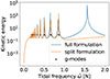Fig. 1. Kinetic energy as a function of the tidal frequency, $\widehat{\omega }$, depending on the formulation used (see plot legends). Crosses correspond to the g-mode frequencies in a cavity (Eq. (B9) of Pontin et al. 2023). Code units are used such that Ro = 1, ωd = 1, and ρ0 = 1.

In addition to the characteristic frequencies of g-modes, the split formulation in the regime where $\widehat{\omega }$ is far from ω_d is similarly able to reproduce the eigenfunction of the resonant mode obtained by the full formulation to very high accuracy, within < 0.01% (left panels of Fig. 2). However, when the tidal forcing frequency $\widehat{\omega }$ is of the same order of magnitude as ω_d, the split formulation cannot reproduce the resonance as it is expected. Indeed, the split formulation cannot reproduce f-modes as the surface needs to be free to capture these.

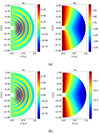Fig. 2. Comparison of the toroidal velocity uϕ for resonant modes in the full formulation (Panel a) and the split formulation (Panel b) for two representative tidal frequencies $\widehat{\omega }=0.1$ (left) and $\widehat{\omega }=1.56$ (right).

3.2. Gravito-inertial modes

We applied the split formulation to the tidal resonance problem for low-frequency modes in rotating NSs, where inertial modes and gravito-inertial modes also come into play. We are therefore in the regime where $\widehat{\omega }\ll {\omega }_d$ and Ω_s, N ≪ ω_d. For our second test, we aimed at probing the impact of the rotation on the gravity modes (i.e., to compare g-modes with gravito-inertial modes) in the right parameter regime. We set Ω_s = 0.0139 ω_d and N = 0.0450 ω_d, respectively.

With these parameters, we computed the kinetic energy of the tidal response (including the equilibrium tide) depending on the tidal frequency for the two formulations. Since we are far from the respective f-mode frequencies, we find that the peak kinetic energy frequencies are identical for both formulations (Fig. 3). We also find that the range of frequency for the gravito-inertial modes is roughly [ − 2Ω_s, N] (that is why the frequency range in Fig. 3 is not symmetrical about 0), which is consistent with the limit ${\widehat{\omega }}_{\max }=N\sqrt{1+4{\mathrm{\Omega }}_s^2/N^2}\approx 1.18N$ found in previous studies (Rieutord 2009; Pontin et al. 2024). By looking at their radial wavelengths, we identify the gravito-inertial modes corresponding to the pure g-modes ₄g to ₁g with slightly smaller frequencies compared to Eq. (33) in the positive frequencies and from ₃g to ₂g modes in the negative frequencies. We find that these negative modes corresponding to n = 2 and n = 3 seem to be roughly at frequencies corresponding to ${\widehat{\omega }}_{{}_n{g}_{-2}^2}\approx -{\omega }_{{}_n{g}_2^2}-\frac{3}{5}{\mathrm{\Omega }}_s$ (i.e., rotation breaks symmetry; in the nonrotating case, negative g-modes are perfectly symmetrical to the positive as in Pontin et al. 2023). The peak at the lower limit of frequencies $\widehat{\omega }=-2{\mathrm{\Omega }}_s$ is related to the negative ₁g mode, but the resonance peak seems not to be reached (not shown here). We also identify a resonant mode close to the frequency of a resonant Rossby mode at $\widehat{\omega }=-0.9\frac{{\mathrm{\Omega }}_s}{3}$. The usual frequency for this resonance is $\widehat{\omega }=-{\mathrm{\Omega }}_s/3$, but it is expected to decrease with α (Ogilvie 2009; Pontin et al. 2024). The identification of the resonant modes with $\widehat{\omega }>{\omega }_{{}_1{g}_2^2}\approx 0.47$ is not straightforward since they cannot be predicted from Eq. (33) and thus are not slightly shifted g-modes. For these other modes, the presence of stratification, which has the effect of shifting resonant peaks (compared to neutrally stratified studies), does not allow clear comparison with any of the regular or singular inertial modes of Ogilvie (2013) or Astoul & Barker (2023). The next resonant peak corresponding to $\widehat{\omega }\approx 0.51$ seems to be a gravito-inertial mode as it has some mixed g-mode and inertial mode features and the n = 1 radial wavelength. This mode is still in the sub-inertial range $\widehat{\omega }<2{\mathrm{\Omega }}_s$ where we expect to find equatorially trapped hyperbolic gravito-inertial modes (as described in Dintrans et al. 1999; Dintrans & Rieutord 2000; Mathis 2009). The higher frequency peaks with $\widehat{\omega }>2{\mathrm{\Omega }}_s$ (in the super-inertial regime) presumably belong to the elliptic gravito-inertial mode family, as described in the aforementioned studies.

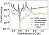Fig. 3. Kinetic energies of tidally excited fluid motions as functions of the tidal forcing frequency, $\widehat{\omega }$, when the full tidal potential is taken into account (blue) and when the tidal forcing is effectively described using the equilibrium tidal flow (orange). The dashed orange line also corresponds to the split formulation but with different boundary conditions (see text), while the solid green line corresponds to the modes obtained only with the effective tidal forcing, ft, due to Coriolis force. Pure g-modes frequencies (black, Eq. (33)) and negative g-modes (red) are designated by a cross. A Rossby mode resonance is highlighted at $\widehat{\omega }=-0.9{\mathrm{\Omega }}_s/3$.

We also compared the kinetic energy to the split formulation but without the forcing term, f_N, in the heat equation; that is, only with f_t, which we call inertial forcing (green line on Fig. 3). Some of the peaks linked to the stable stratification and g-modes cannot be seen anymore, are strongly mitigated (especially for low frequency), or change geometry completely as shown on the ₁g mode (left panel of Fig. 4). Without it, it corresponds to having gravito-inertial modes with the gravity component only secondarily excited by the effective Coriolis forcing. For example, the mode at $\widehat{\omega }=0.777N$ is well recovered with only the effective Coriolis forcing although the amplitude is divided by two (right panel of Fig. 4 but at the frequency of the ₁g mode the mode is completely different (left panel of Fig. 4).

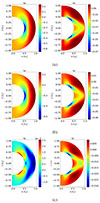Fig. 4. Comparison of two gravito-inertial modes along ϕ = 0 for the different formulations. The first mode, with $\widehat{\omega }=0.421N$, corresponds to the 1g22 mode impacted by the rotation, while the second one is closer to an inertial or gravito-inertial mode, $\widehat{\omega }=0.777N$. Velocities are given in units such that Roωd = 1.56 × 1010 cm s−1. Left: Toroidal velocity uϕ at ϕ = 0 for $\widehat{\omega }=0.421N$ in the full formulation (Panel a), split formulation (Panel b) and with only effective Coriolis forcing (Panel c). Right: Toroidal velocity uϕ at ϕ = 0 for $\widehat{\omega }=0.777N$ in the full formulation (Panel a), split formulation (Panel b) and with only effective Coriolis forcing (Panel c).

For all the peaks below $\widehat{\omega }<0.5N$, the kinetic energy for both formulations agrees within < 1%, but there are some differences with the full formulation as the amplitude of the velocity becomes lower in the split formulation for the tidal frequencies, $\widehat{\omega }$, higher than the BV frequency. This means that some tidal response seems to not be captured by the split formalism when further away from the g-mode or gravito-inertial mode frequencies. In order to investigate this effect, we looked at the resonant mode for two different tidal forcing frequencies. For $\widehat{\omega }<N$, the gravito-inertial mode velocity is reproduced within 0.5% by the split formulation (two upper left panels of Fig. 4). We can also see the impact of the rotation, which makes the mode more cylindrical than the spherical symmetry of pure g-modes. For $\widehat{\omega }\approx N$, the toroidal velocity is not exactly reproduced by the split formalism, and the kinetic energy seems to decrease with increasing tidal frequency, since we left the allowed frequency range for gravito-inertial waves to be excited, and the equilibrium tide is no longer negligible. This behavior can be explained by differences in the boundary conditions. Indeed, when outside of the resonant peaks, the amplitude of the equilibrium tide u_e cannot be neglected compared to those of the dynamical tide u. This leads to a difference in boundary conditions as the full formulation solves the equations for both tides u + u_e, while the split formulation solves the equation for the dynamical tide u. In order to compare the two formalisms, we artificially accounted for the impact of the equilibrium tide by changing our boundary conditions for the viscous rate tensor to τ_ν, rθ(u) =  − τ_ν, rθ(u_e) and τ_ν, rϕ(u) =  − τ_ν, rϕ(u_e). Applying these changes, we recovered the results from the full formulation within < 0.05% (Fig. 5).

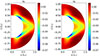Fig. 5. Toroidal velocity, uϕ, with $\widehat{\omega }=0.777N$ in the full formulation (left), and in the split formulation (right) with modified non stress-free boundary conditions (see text).

Since the split formulation has two effective forcing terms, f_t and f_N, we can compute the power associated with both to assess their importance. Figure 6 shows the different components of the power of the forcings and the thermal and viscous dissipation due to the tidal flows. We first verified that the balance of Eq. (28) is verified and the error that depends on resolution is around 10⁻⁷%. For almost all the modes, the power of the forcing, f_N, due to the advection of the buoyancy variable gradient dominates, which is expected since we are in the regime N > Ω_s. For large Pr, this statement may be even more true since thermal dissipation will be less important. The power of the forcing f_N also dominates at a resonant Rossby frequency $\widehat{\omega }=-{\mathrm{\Omega }}_s/3$ where the contribution of the effective Coriolis forcing is the strongest for negative frequencies and is around P_Cor ≈ 0.4P_buoy. The only exception is of the gravito-inertial modes found for $\widehat{\omega }=0.777N$, described before. We also find that the power due to the Coriolis effective forcing f_t alternates between negative and positive values, while the total power is always positive. This might be linked to the splitting due to rotation of the gravity modes m = ±2.

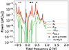Fig. 6. Power and dissipation balance of the tidally excited fluid motions as a function of the tidal forcing frequency, $\widehat{\omega }$, with the split formulation of the tidal forcing with N/Ωs = 3.24. Similar to Fig. 3, the pure g-mode frequency (Eq. (33)) is designated by crosses.

The case of pure inertial modes with the effective body force f_t has been well studied and therefore needs no testing. Overall, these tests show that the split formulation with the two forcing terms is able to obtain well the resonant gravito-inertial modes without having a free surface implemented, as long as the mode frequency is much smaller than ω_d.

4. Nonlinear simulations of gravito-inertial modes

As the orbital separation a shrinks with time due to the emission of GWs, the tidal forcing frequency and amplitude increase, and nonlinear effects can start to be important for the dynamics of the resonance. In this section, we discuss how we tested and studied the importance of nonlinear effects for binary NSs. In particular, we look at the nonlinear saturation of the gravito-inertial modes (i.e., when the nonlinear simulation reaches an average steady state).

We implemented the split formulation in the code MagIC with the stress-free boundary conditions applied to the dynamical tide u, since it does not change results for resonant modes compared to stress-free boundary conditions applied to both equilibrium and dynamical tides. In a similar fashion to Astoul & Barker (2023), we also chose to neglect some nonlinear interactions between the equilibrium and dynamical tides. Indeed, our model uses a non-deformed spherical shell, which in the presence of mixed (equilibrium-dynamical) nonlinear terms would lead to a nonvanishing equilibrium tide at the surface u_e ⋅ n ≠ 0. In this case, the advection of the dynamical flow by the equilibrium flow can artificially generate angular momentum and spin up the star. We, therefore, neglected this advection term to avoid this setup artifact and because it is justified in the astrophysical regime (see discussion of Astoul & Barker 2022). For the saturation of the flow, we only considered the nonlinear effects of the dynamical tide on itself (u ⋅ ∇)u. This can be justified in cases where mode wavelengths are much smaller than the radius of the cavity.

We used this implementation to run several simulations for a NS binary of two solar masses, adopting an initial rotation of Ω_s = 100/π Hz to continue the comparison as in the previous section. One notable difference is that, in this section, the gradient of the buoyancy variable $\frac{d\stackrel{\sim }{b}}{\mathit{dr}}\propto \frac{N}{g}$ is constant instead of the BV frequency for the sake of simplicity. The BV frequency in this case depends on the radius, and N(r) = Nr and g = g_or. This leads the linear g-modes to have smaller amplitudes and smaller resonant frequencies compared to the pure g-modes case shown in Sect. 3.1 with constant BV frequency.

For the amplitude of the tidal force, we chose the tidal parameter to reflect the situation of having $\widehat{\omega }\approx N$ so as to study the resonance of gravito-inertial modes, which gives a tidal amplitude of C_t ≈ 10⁻³ for N = 102.87 Hz, Ω_s = 100/π Hz, and ω_d = N/0.0450. In order to investigate differences in nonlinear effects between the different modes, we kept the tidal amplitude constant for all simulations in this section. Note that we would have $C_t=\sqrt{6\pi /5}ϵ\propto {({\mathrm{\Omega }}_o/{\omega }_d)}^2$ (neglecting the real part of the Love number) in the realistic case (see Sect. 5).

4.1. Linear and nonlinear comparison

To be confident in our nonlinear simulations, we first compared the MagIC simulation results to the linear results. We ran the linear code for $\widehat{\omega }\in [-2{\mathrm{\Omega }}_s,2N]$ with a frequency resolution N_freq = 500, while N_freq = 100 for the nonlinear simulations. Figure 7 shows the total kinetic energy of the different modes for both the linear code and the nonlinear code MagIC. Overall, we find a good agreement between the two codes for many resonant modes, and the comparison of one of these cases can be seen for the structure and amplitude of the ₃g mode (first mark furthest to the left on Fig. 7) in Fig. 8. The mode is deformed by rotation and becomes more cylindrical compared to a pure g-mode (see left panels of Fig. 2 for a pure g-mode at a different frequency). We still notice small differences for some resonance modes, but such effects may stem from the two different frequency resolutions or due to small nonlinear effects.

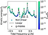Fig. 7. Kinetic energy along the tidal frequency, $\widehat{\omega }$, for the linear code (dashed lines) or the nonlinear simulations (scatter points) with Ct = 10−3. The color scale of the nonlinear simulations corresponds to the ratio of the axisymmetric kinetic to the total kinetic energy.

Fig. 8. 3g-mode resonance with $\widehat{\omega }=0.126N$ at ϕ = 0 in the case of small rotation (N/Ωs = 3.24). Results of the linear code are shown on the left, while that of the nonlinear code are on the right; notice the difference in the color bar for each panel.

To quantify the importance of nonlinear effects, Fig. 7 shows the ratio of the axisymmetric-to-total kinetic energy in these simulations. It clearly shows that with the strongest resonance modes, a m = 0 zonal flow component emerges in addition to the forced m = 2 component. This means that nonlinear effects are stronger for these modes. It is not the only criterion, though, as the ₂g₂² mode has the highest percentage of axisymmetric energy, while the ₁g₂² mode has the highest mode energy.

4.2. Nonlinear saturation

The previous section showed that for C_t = 10⁻³, the nonlinear saturation of the kinetic energy matches the linear one. In this section, we examine this assumption to see if it still holds for the strongest resonances. Since nonlinear effects could become important, we also compare the linear and nonlinear simulations for cases with the highest percentage of axisymmetric energy and the highest absolute axisymmetric energy. They correspond to the ₂g- and ₁g-modes, as discussed above. We first checked that in the case of C_t = 10⁻⁹, the kinetic energy of both nonlinear simulations agrees with the associated linear simulations within a relative error <  10⁻⁶. Figure 9 compares the time evolution of the nonlinear simulations and the saturated energies predicted by the linear calculations for both modes. We find that the non-axisymmetric energy of the ₂g-mode agrees well with the linear kinetic energy. We note that its total saturation is slightly increased by the axisymmetric energy, which is 10% of the total energy. In the case of the ₁g-mode, the nonlinear saturation is lower by a factor of 3. This means that the saturation mechanism differs from the linear theory for this mode. It is possible that we only see it for this mode due to it having the strongest amplitude.

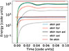Fig. 9. Time evolution of the kinetic energy for the nonlinear simulations of 1g and 2g modes compared to the linear results (dashed red lines). The lines above correspond to the 1g mode with $\widehat{\omega }=0.348N$. The lines below correspond to the 2g− mode with $\widehat{\omega }=0.186N$, which are rescaled by a factor of 0.1 for improved visibility.

Figure 10 compares the non-axisymmetric and axisymmetric toroidal velocity of the two modes to see the impact of the nonlinear saturation. We find that axisymmetric rotation, decreasing with cylindrical radius, is generated for both modes. We expect that the differential rotation emerges due to nonlinear processes such as tidal wave-wave interactions (m = 2 and m = −2 nonlinear coupling to form an m = 0 mode, as explained in Barik et al. 2018; Astoul & Barker 2022, for inertial waves) and/or wave breaking as in Barker & Ogilvie (2010) in a 2D cylindrical geometry, Barker (2011) in a 3D box, and Guo et al. (2023) in a 2D circular cavity (see also, e.g., Semin et al. 2016, for experimental generation of a mean flow by internal gravity waves). In the latter, the geometrical focusing of gravity waves launched from the surface toward the center generates differential rotation from inside out by wave breaking (or weak linear damping) of (subcritical) waves and their progressive deposition of angular momentum. Wave breaking is observed when the amplitude of the wave is high enough to overturn the stratification (Barker & Ogilvie 2010; Barker 2011). We therefore applied the following criterion with the radial displacement, ξ_r, and wavenumber, k_r, described in the aforementioned papers for wave breaking to our simulations:

$$\begin{array}{c}\hfill {\xi }_r{k}_r>1.\end{array}$$(34)

Fig. 10. Strongest two g-mode resonances and their nonlinear saturation in the case of small rotation (N/Ωs = 3.24). Non-axisymmetric (left) and axisymmetric (right) toroidal velocity uϕ for the 2g mode (Panel a) and for the 1g mode (Panel b).

We find that the wave is not strong enough to have wave breaking in these simulations. The presence of both Coriolis and buoyancy forces promotes a mix between cylindrical and spherical geometry of the mean flow (which is reminiscent of latitudinal differential rotation produced in Fig. 6 of Barker 2011). In proportion to the amplitude, the differential rotation is stronger for the ₂g-mode.

The emergence of differential rotation supports our hypothesis for the resonant mixed gravito-inertial modes to be able to amplify some ambient magnetic field through winding in a way that is qualitatively similar to that studied by Astoul & Barker (2025). In future work, these results should be checked for different BV frequencies that are more realistic for astrophysical sources to assess the impact of the differential rotation amplitude.

5. An astrophysical application: Gravito-inertial modes in a neutron star binary

Depending on the stellar spin, the eigenfrequencies of gravito-inertial modes imply that they may become resonant some seconds prior to merger in a binary neutron-star inspiral. Because of their polar character, the leading-order overlap integrals and hence amplitudes may also be sizeable. These aspects together indicate that these modes may be important in the description of mergers for a few reasons:

• A leading theory for explaining the ignition of GRB precursor flares, seen in ≲5% of mergers (Coppin et al. 2020; Wang et al. 2020), is that of crustal failure: resonant modes exert strain on the ion lattice defining the crust, which may exceed its elastic maximum if the mode amplitudes are large enough. Such an overstraining relieves the star of some magnetoelastic energy, which can fuel a gamma-ray flash (Tsang et al. 2012). Previous estimates using a linear, general-relativistic (GR) framework (Passamonti et al. 2021; Kuan et al. 2021b; Suvorov et al. 2022) found that some g-modes may exceed modern estimates for polycrystal strain maxima (Baiko & Chugunov 2018; Baiko 2024); a direct comparison is made with our nonlinear models in Sect. 5.1.

• Energy may be siphoned from the orbit into the kinetic energy of the modes, leading to GW dephasing. Linear theory predicts that while the dephasing due to gravity(-inertial) modes is unlikely to be visible to current interferometers, it may be relevant for next-generation ones (Ho & Andersson 2023, see also Suvorov et al. 2024b). In general, however, we expect that treating mode excitations via nonlinear perturbation theory would favor measurability since amplitudes in post-resonance regimes do not remain constant as in linear theory (Yu et al. 2024; Kwon et al. 2024, 2025). In addition, the onset of GW dephasing depends on the resonance timing, which can differ between linear and nonlinear models, as explored in Sect. 5.1. Deducing their nonlinear saturation amplitudes is a necessary step toward providing realistic assessments of dephasing; such a comparison is made in Sect. 5.2.

• Observations of nonthermal GRB precursors and other aspects (see, e.g., Xiao et al. 2024) hint that some magnetar-like objects participate in a rare subclass of mergers. This is difficult to reconcile with the fact that Ohmic decay times are thought to be much shorter than a characteristic inspiral time (e.g., Pons & Viganò 2019). One solution is that actually strong fields are not preserved but rather generated prior to coalescence by a mode-driven dynamo, as suggested by Suvorov et al. (2024a). The validity of this scenario depends on microphysical specifics as well as the mode properties; some MHD aspects of this in the context of the simulations presented here are discussed in Sect. 5.2.2.

In this section, we return to a closer examination of the astrophysical elements of a NS binary. Accordingly, we changed our model and considered a more standard NS of 1.6 M_⊙, anticipating that for objects with non-negligible spin, some prior epoch of accretion may have increased the birth value. We adopted a radial profile for the BV frequency inspired by a realistic model of the NS from Suvorov et al. (2024a). We neglected (physical) discontinuities arising in the BV frequency in our “crustal cavity” due to different layers of nuclear composition, as the results were very likely to change with density variations between the core and the crust. The study of core-crust interfacial modes (i.e., i-modes; Tsang et al. 2012) due to these discontinuities is left to future studies. In Fig. 11 we show the smoothed BV frequency: it is visually identical to that predicted by the GR calculations except in the crust. The other main difference in our nonlinear simulations from the linear calculations in Suvorov et al. (2024a) would be that the density is still kept constant, as we first aimed at understanding nonlinear effects in a simpler setup.

Fig. 11. BV frequency for a 1.6 M⊙ NS with the APR4 EOS, giving a radius of Ro = 11 km from Suvorov et al. (2024a). The orange line is the profile that is used in the Newtonian simulations presented here (see main text for details). For reference, we overlay the BV frequency of the setup in Sect. 4 (dashed line).

5.1. Comparison to GR linear calculations

First, before treating rotation self-consistently, we directly compared GR linear calculations to our linear ones to estimate the impact of our numerical hypotheses. To compute these modes, we used a radius ratio of α = 0.1 and the smooth BV profile from Fig. 11. As it turns out, the agreement is encouraging: the resonant frequencies are only slightly shifted to lower or higher values by 3.5% and 2.3% for the ₂g and ₁g modes, respectively.

The radial eigenfunctions between the two also agree well until a radius of ≈0.8 R_o, where the impact of the density gradient and, subsequently, the discontinuities become more important (see Fig. 12 for the case of u_ϕ, which corresponds to u^ϕ in GR calculations). In terms of amplitudes, the Newtonian ₁g and ₂g modes are rescaled by a factor of ∼0.02 and ∼0.0175 for the radial profiles to match, respectively. This rescaling is due to the way the linear modes are computed: in the GR case, the resulting mode amplitude is determined by the resonance time window, while, in the Newtonian case, the mode amplitude is determined by the balance between the tidal power and the dissipation through the diffusivities. The rough agreement between the rescaling factors shows that the results from the Newtonian case in the core are consistent with the GR linear calculations. We can therefore use the smooth BV frequency to study the resonant modes and their nonlinear saturation. However, the results will be mostly relevant to core-like regions of the NS, and a proper treatment of the density and BV discontinuities is required to study quantitatively the modes in the crust.

Fig. 12. Toroidal velocity for 1g22 and 2g22 modes. Solid lines represent the cases as those in Fig. 1 of Suvorov et al. (2024a).

5.2. Nonlinear saturation of the strongest resonance

In this section, we show how we tested the impact of rotation on the ₁g and ₂g modes that generated the strongest nonlinear differential rotation in Sect. 4.2. We first began with the ₂g mode as it has the lowest mode amplitude. Thus, nonlinear effects were expected to be smaller, and we therefore considered three different rotation rates, Ω_s ∈ [0, 100/π, 100] Hz (i.e., astrophysically corresponding to irrotational, moderate, or “recycled” objects). To keep the viscosity the same as previous simulations, the same Rayleigh number Ra was maintained, but the Ekman number varied from Ek = 6.2 × 10⁻⁵ to Ek = 1.99 × 10⁻⁵ in the slow and fast rotating cases (note that the Ekman number is not defined for Ω_s = 0.0). With the new BV profile, which is normalized at the outer boundary, the Rayleigh number is now Ra = −5.1 × 10¹⁰. For the same tidal forcing frequency, the orbital frequency Ω_o is effectively higher since the spin of the NS is increased, and we thus obtain a larger tidal amplitude parameter, ϵ. Our strategy is to first use the linear code to compute the resonant frequencies, which is then fed into the nonlinear code to compute the saturation amplitudes. As one of our motivations is to investigate the strength of the magnetic field that could be theoretically generated by differential rotation, energies are shown in ergs and compared to the strength of a magnetic field that would have the same energy as the flow kinetic energy. This comparison is done by using the energy of a uniform 10¹⁴ G magnetic field, $E_{B14}=\frac{1}{8\pi }\left[{({10}^{14}\mathrm{G})}^2\mathrm{V}\right]=2.27\times {10}^{45}$ erg, where $V=\frac{4\pi }{3}(1-{\alpha }^3)R_o^3$ is the volume of the domain.

5.2.1. ₂g mode

We first describe the ₂g mode for different rotation rates, Ω_s ∈ [0, 100/π, 100] Hz. For these spins, the tidal forcing frequencies of the ₂g mode are respectively $\widehat{\omega }/N\in [0.146,0.132,0.127]$, while the tidal dimensionless amplitudes are C_t = 9.3 × 10⁻⁴ and C_t = 4.1 × 10⁻³ for the two rotating cases. In order to compare the efficiency of the nonlinearities in the nonrotating case, we manually adjusted the tidal amplitude in the nonrotating case to the fast rotating case, namely C_t = 4.1 × 10⁻³ instead of the realistic one C_t = 5.29 × 10⁻⁴. This allows us to effectively mimic nonlinear effects at lower viscosities since the amplitude of the resonant modes increases with decreasing viscosity (in the linear regime, e.g., Ogilvie 2009; Pontin et al. 2023). Figure 13 shows the time evolution of the different kinetic energies, which for all simulations would be enough to generate a magnetic field stronger than 10¹⁴ G if we assume that this kinetic energy would be subdivided through dynamical means into equal parts kinetic and magnetic energy (equipartition). We see that nonlinearities become relevant for both modes after less than 1 s of evolution. The nonlinearities for the ₂g mode and their impact are mostly seen in the toroidal kinetic energy, which is expected physically as zonal flows mainly develop in the azimuthal direction. For Ω_s = 100/π Hz, the poloidal kinetic energy dominates and nonlinear effects are weaker than in the other case due to the lower tidal amplitude. We find that the axisymmetric energy represents ∼20% of the total kinetic energy. This is higher than but still consistent with the results of the previous section. For a faster star with Ω_s = 100 Hz, the toroidal component becomes dominant and the axisymmetric kinetic energy is comparable to the non-axisymmetric energy, representing ∼50% of the total energy.

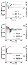Fig. 13. Time evolution of the kinetic energy for the 2g mode for Ωs = 100/π Hz, (top), Ωs = 100 Hz (middle), and Ωs = 0 with an increased tidal amplitude (bottom).

To understand whether this increase is due to rotation or the tidal amplitude, we compare it to the nonrotating case with the same tidal amplitude. We find a striking difference for Ω_s = 0: the nonlinear effects become important much faster, and the axisymmetric toroidal velocity becomes dominant after 1 s. The toroidal kinetic energy saturates at a higher level compared to the other two rotating cases. This different evolution may be due to the fact that the amplitude of linear g-modes also saturates at greater values with lower rotation because of overlap integral properties (see Fig. 6 of Pontin et al. 2024). For a given tidal amplitude, the nonlinear effects are therefore more important with lower rotation, which is what we observe in our simulations.

To compare the nonlinear effects for the three cases in more detail, we look at the kinetic energy spectra along degrees, ℓ, and orders, m. The m = 2 mode would dominate for purely linear solutions, and the ℓ = 2 mode should dominate for pure g-modes as the different ℓ modes are only coupled by the Coriolis force. Note that ℓ = 2 is also dominant for linear inertial waves because the tidal potential has a ℓ = 2 geometry. In addition, we expect to have even ℓ modes dominating for the poloidal field and odd ℓ modes for the toroidal field due to the equatorial plane symmetry of the equilibrium tide used for the effective forcing, assuming this persists nonlinearly. We see these behaviors in the spectrum depending on the ℓ modes of the two rotating cases and, to a lesser extent, in the nonrotating case too (left panels of Fig. 14). As nonlinear effects become more important (i.e., at larger tidal amplitudes), the spectrum gets extended to higher degrees ℓ.

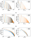Fig. 14. Kinetic energy spectra of the 2g-mode resonance for Ωs = 100/π Hz, (top), Ωs = 100 Hz (middle), and Ωs = 0 with an increased tidal amplitude (bottom). The left panels denote kinetic energy integrated over r and m, while varying ℓ; and the right panels are integrated over r and ℓ, while varying m. The kinetic energy is in viscous units. The tidal amplitude is Ct = 9.3 × 10−4 in Panel a, Ct = 4.1 × 10−3 in Panel b and in Panel c.

For the spectrum along order m, we see that the m = 2 and the m = 0 modes dominate for the poloidal component and for the toroidal component, respectively (right panels of Fig. 14). We also see that odd orders m are nonrelevant for the rotating cases and only start to become relevant for the nonrotating case with the strongest nonlinear effects, while remaining below even modes. We see that the amplitude of the toroidal mode m = 0 becomes more and more dominant as the tidal amplitude increases, which is consistent with the ratio of axisymmetric energy in the time evolution. The m = 0 mode of the poloidal component stays much lower than the m = 2 mode.

To confirm the importance of the m = 0 mode of the velocities, we show snapshots of u_r and u_ϕ in the equatorial plane for the three different cases in Fig. 15. In the rotating cases, we see that the modes are quite similar: for u_r, the differences between the maximum amplitude of the dominant m = 2 mode are within 30%, and there is only a small difference in geometry close to the equatorial plane (not shown here). There are more differences for u_ϕ as its amplitude increases with rotation and tidal amplitude. The increase in the axisymmetric component with tidal amplitude can also be seen as the negative amplitude close to the inner core neighbors zero in the fast rotating case. In a similar fashion, the difference between positive and negative amplitudes of u_ϕ close to the outer boundary is lower in the fast rotating case. This means that the inner region is spun up and the outer region is instead spun down for this particular resonance.

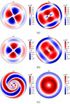Fig. 15. Velocity flows (in CGS units), ur (left) and uϕ (right), of the gravito-inertial 2g mode in the equatorial plane for Ωs = 100/π Hz (top), Ωs = 100 Hz (middle), and Ωs = 0 with an increased tidal amplitude (bottom). The tidal amplitude is Ct = 9.3 × 10−4 in Panel a, Ct = 4.1 × 10−3 in Panel b and in Panel c.

The nonrotating case is both qualitatively and quantitatively different as compared to the rotating cases: for u_r, the m = 2 mode is still dominant but the number of radial nodes is increased, especially in the inner region, and the amplitude is lower by a factor of ∼5. For u_ϕ, the m = 0 mode is dominant with the addition of “spiral arms” that appear similar to a superposition of m = 2 and m = 1 modes (and/or traveling waves). The amplitude of u_ϕ is also ∼4 times stronger compared to the rotating cases. This strong spin-up in the inner region might explain why different radial modes are excited for this nonrotating case. Indeed, the spin-up leads to a rotation rate of Ω_s,spin−up ≈ 20 Hz, which would modify the tidal forcing frequency from $\widehat{\omega }=0.127N$ to $\widehat{\omega }\approx 0.038N$. This would lead to the excitation of higher radial-number gravity-modes and could explain the splitting of the domain into two regions, where the excited modes appear more similar to ₃g (₁g) in the inner (outer) region. The spin-up would also increase viscous and thermal damping in the inner regions since the modes are of shorter length scales in these regions, which possibly explains why Fig. 15 (Panel (c)) appear as (traveling) spiral waves. These spiral waves look similar to those of the 2D simulations of Guo et al. (2023) when tidal amplitude forcing is high (implying strong nonlinear effects). They find that angular momentum is carried by an inwardly traveling wave and deposited due to wave breaking at the center of a circular cavity, creating an expanding critical-layer from the inside out. We also observe that the radial wavelength decreases toward the center, which may lead to wave breaking as the stability criterion with the radial displacement ξ_rk_r ≪ 1 becomes marginally wrong.

We can confirm the overall spin-up in the domain for all three cases by looking at the toroidal velocity u_ϕ in the meridional plane (Fig. 16). First, we see that the non-axisymmetric contribution is stronger than the axisymmetric contribution at a smaller tidal amplitude as nonlinear effects are less important. When modes become more nonlinear, the axisymmetric part becomes of the same order as the non-axisymmetric component and even dominates for the nonrotating case with increased amplitude. By increasing rotation, the modes become more cylindrical as it can be seen in the Ω_s = 100 Hz case, while they are spherical when Ω_s = 100/π Hz and Ω_s = 0. In the nonrotating case, we also see the same radial geometry observed in the equatorial plane: the gravity ₂g mode seems to be split into a ₃g mode in the inner region and ₁g mode in the outer region. We computed the vertical angular momentum following

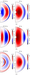Fig. 16. Velocity flow (in CGS units) of the gravito-inertial 2g mode in the meridional plane for Ωs = 100/π Hz, (top), Ωs = 100 Hz (middle), and Ωs = 0 with an increased tidal amplitude (bottom). Non-axisymmetric (left) and axisymmetric (right) toroidal velocity uϕ of the 2g mode for Ωs = 100/π Hz and Ct = 9.3 × 10−4 (Panel a), for Ωs = 100 Hz and Ct = 4.1 × 10−3 (Panel b) and for Ωs = 0 with a tidal amplitude of Ct = 4.1 × 10−3 (Panel c).

$$\begin{array}{c}\hfill L_z={\displaystyle {\int }_V}{(r\sin \theta )}^2\mathrm{\Omega }\mathrm{d}V,\end{array}$$(35)

with Ω = u_ϕ/(r sin θ), to estimate the spin-up in the inner half of the domain V from r = 0.1R_o to r = 0.55R_o. We then estimated the solid body rotation rate at the end of the simulation Ω_s, end that would correspond to this angular momentum, via

$$\begin{array}{c}\hfill {\mathrm{\Omega }}_{s,\mathrm{end}}=\frac{L_z}{{\displaystyle {\int }_V}{(r\sin \theta )}^2\mathrm{d}V}·\end{array}$$(36)

We find that Ω_s, end ∈ [21.58 Hz, 1.0476Ω_s, 1.042Ω_s] for initial values Ω_s ∈ [0, 100/π, 100] Hz. With stronger nonlinear effects (i.e., stronger tidal amplitude and/or reduced rotation), the absolute value of the spin-up is stronger as it goes from Ω_s, end − Ω_s = 1.5 Hz to 21.58 Hz.

5.2.2. ₁g mode

Using the same strategy, we turned our attention to ₁g modes. The tidal forcing frequencies of the ₁g mode are $\widehat{\omega }\in [0.235N,0.218N,0.132N]$ for Ω_s ∈ [0, 100/π, 100] Hz, and the tidal dimensionless amplitudes are C_t = 1.6 × 10⁻³ and C_t = 5.3 × 10⁻³ for the two rotating cases. As for the ₂g mode, we used the same tidal amplitude in the nonrotating case as in the more-rapidly rotating case C_t = 5.3 × 10⁻³ instead of the realistic one C_t = 1.36 × 10⁻³. Figure 17 shows time evolutions for the different kinetic energies, which for all simulations would be enough to generate a magnetic field stronger than 10¹⁵ G assuming equipartition. The nonlinearities become relevant for the two modes after less than 1 s after initialization.

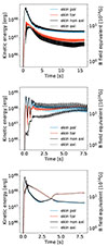Fig. 17. Time evolution of the kinetic energy for the 1g mode for Ωs = 100/π Hz (top), Ωs = 100 Hz (middle), and Ωs = 0 with an increased tidal amplitude of Ct = 5.3 × 10−3 (bottom).

The evolution of the ₁g modes is quite different from that of the ₂g mode. After a first growth, some fast oscillations of the kinetic energy appear. These oscillations may indicate that the ₁g mode is subject to parametric instabilities or corotation resonance instabilities. Before looking more into the instabilities, we note that similar results to those obtained for the ₂g mode are found for the importance of nonlinear effects. Indeed, for Ω_s = 100/π Hz, the poloidal kinetic energy dominates, and the axisymmetric energy represents again around ∼20% of the total kinetic energy. For Ω_s = 100 Hz, the nonlinear effects are even stronger, as the axisymmetric energy represents ≈50% of the budget. In addition, the toroidal and poloidal components contribute evenly to the total kinetic energy at the end of the simulation. To understand the impact of rotation and tidal amplitude, we compared this evolution with that of the nonrotating case with the same tidal amplitude. We find a critical difference for Ω_s = 0: the nonlinear effects become important sooner in the evolution, and the axisymmetric toroidal kinetic energy becomes dominant after 1 s. The time evolution for the nonrotating case is quite interesting, as the first growth is higher than in the other cases but it drops quicker, until stabilizing after 4 s. The first decreasing part is due to the evolution of an instability, as we see small oscillations in the poloidal kinetic energy until the m = 2 mode grows again and dominates the energy contribution for the second part after 4 s.

To better understand these three simulations, we looked at the kinetic energy spectra along degrees, ℓ, and orders, m, at the end of the time evolution (Fig. 18). The difference with the ₂g mode is quite clear as there are no patterns between odd and even degrees. This means that equatorial symmetry is broken by an instability. For the two rotating cases, the spectrum is continuous, meaning that nonlinear effects are strong. This can be seen as well on the order spectrum, where, for the rotating cases, the dominant mode for the poloidal component is not the m = 2 mode (of the initial tidally forced waves) but the m = 1 mode. For the toroidal component, there is also a strong m = 1 mode but the m = 0 mode is dominant. The emergence of this m = 1 mode indicates that an instability appears in this simulation. In all three cases (with and without rotation), the energy cascade from high to small spatial scales approaches a scaling ∝l⁻³ at low and moderate spherical harmonics degrees³, rather than a less steep scaling ∝l^−5/3 as for a Kolmogorov spectrum. This is reminiscent of weak or wave turbulence as described for instance in Galtier (2003), Le Reun et al. (2020) for inertial waves, and in Bellet et al. (2006), Le Reun et al. (2018) for internal gravity waves. In our simulations, the onset of turbulence may be driven by the energy cascade toward different parity modes and smaller spatial scales, as found in other setups of unstratified hydrodynamical turbulence driven by triadic resonances of inertial waves (see for instance Barik et al. 2018, 2024).

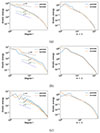Fig. 18. Similar to Fig. 14 but for the 1g-mode. We compare the spectrum to several wave scaling laws corresponding to ℓ−5/3, ℓ−2, and ℓ−3 (dotted lines) from internal wave turbulence (Le Reun et al. 2018, 2020). The tidal amplitude is Ct = 1.36 × 10−3 in Panel a and Ct = 5.3 × 10−3 in Panel b and Panel c.

To characterize the instability and the oscillations that appear for the rotating simulations, we performed a Fourier transform of the poloidal scalar potential W(l, m, r_FFT) at midpoint of the domain r_FFT = 0.55 for the different main modes for the slower and faster rotating cases and nonrotating case (Fig. 19). For both rotating cases, we find that the dominating component is the (l, m) = (1, 1) mode and the oscillations of this mode are divided into two frequencies ω₁ and ω₂. We call ω₁ the main frequency at ω₁ = 63.098 Hz and ω₁ = 58.184 Hz, for Ω_s = 100/π Hz and Ω_s = 100 Hz, respectively. We also see that the second main mode corresponds to the expected (l, m) = (2, 2) mode, but additional modes are also excited, including a number of even ℓ + m modes due to symmetry. In contrast, odd ℓ + m modes are excited for the toroidal velocity potential, especially in the highest-rotation case where the tidal amplitude and nonlinear effects are stronger. The (l, m) = (2, 2) is excited at the tidal forcing frequency $\widehat{\omega }$ and the (l, m) = (4, 4) is excited at its superharmonics $2\widehat{\omega }$ in the fast rotating case only. The second tallest peak of the (l, m) = (1, 1) mode is at the frequency ${\omega }_2=\widehat{\omega }-{\omega }_1$. Therefore, it seems that the m = 1 mode is growing at the expense of the main m = 2 forcing mode, which would explain why the latter is not dominant anymore (compared to simulations without the instability). All these observations provide clear evidence for triadic resonances or parametric instabilities since all of the excited modes can be recovered by a linear combination of $\widehat{\omega }$ and ω₁ and their corresponding degrees and orders. In particular, we recover the modes (l, m) = (3, 3) = (2, 2)+(1, 1) = (4, 4)−(1, 1), with both excited frequencies ${\omega }_{3,3}\in [\widehat{\omega }+{\omega }_1,2\widehat{\omega }-{\omega }_1]=\widehat{\omega }+{\omega }_2$. These types of instabilities have been theorized and observed in 3D nonlinear simulations in shells for inertial waves (e.g., Kerswell 1999; Barik et al. 2018; Astoul & Barker 2022), and also analyzed through 2D simulations and weakly nonlinear calculations for pure gravity waves in stellar radiative cores (e.g., Barker & Ogilvie 2011; Weinberg et al. 2012, 2024; Essick & Weinberg 2016).

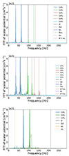Fig. 19. Fourier transform of the poloidal velocity potential, W, showing the different main modes for Ωs = 100/π Hz (top), Ωs = 100 Hz (middle), and Ωs = 0 (bottom). We obtain ω1 ∈ [63.1, 58.2, 73.7] Hz and ${\omega }_2=\widehat{\omega }-{\omega }_1$. In the nonrotating case, the FFT in the first phase, t ∈ [0, 4] s, is plotted with the dotted line, while the second phase, t ∈ [4, 10] s, is plotted with solid lines.

In the fast-rotating case, we can see the impact of rotation as the main frequencies are split between a slightly higher frequency and a lower frequency. The new peaks appearing with fast rotation can also be recovered by a linear combination of the $\widehat{\omega }$ and ω₁ and their corresponding split frequencies. The split frequencies may correspond to ω_split = ω_i ± mδω_s where δω_s/Ω_s is the normalized differential rotation. If we set m = 2 (which corresponds to the pair of largest split frequencies, in green in Fig. 19), we then deduce that δω_s/Ω_s ≈ 0.023 for all modes i. This reasoning works in the case where only one mode is split, and then leads to the emergence of other modes through triadic resonances involving linear combinations of azimuthal degree, orders, and frequencies. It is strongly corroborated by the fact that the splitting is the same for all modes (contrary to the case where different modes are split such that the splittings depend on their azimuthal degree and order as described in Aerts et al. 2010).

To spatially visualize the triadic resonances, we first looked at snapshots of the radial u_r and toroidal u_ϕ velocity in the equatorial plane (Fig. 20). As expected from previous diagnostics, the m = 1 mode is clearly dominant for the two rotating cases. The velocity components u_r and u_ϕ are overall stronger in the case with higher rotation. The radial structure in the two cases is similar, with the half-wavelength mode dominating for u_r and the full-wavelength one for u_ϕ, as expected for the ₁g mode. Some small-scale structure with strong amplitude is present close to the inner boundary. One could think that the inner boundary, and the development of a Stewartson layer at the inner tangent cylinder (Stewartson 1966; Barik et al. 2018, 2024), is at the origin of this parametric instability, but we also observe a similar growing ℓ = m = 1 mode in a test simulation with a full sphere (not shown here). The increase in nonlinear effects with the fast rotation can also be seen in u_ϕ as the m = 1 mode is less important compared to the m = 0 mode. In this case, the zonal flow looks more similar to the one for the ₂g mode, where the inner region is spun-up and the outer region is spun-down.

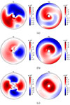Fig. 20. Similar to Fig. 15 but for 1g modes. The tidal amplitude is Ct = 1.36 × 10−3 in Panel a and Ct = 5.3 × 10−3 in Panel b and Panel c.

In the nonrotating case, we find similar results to the previous ₂g mode, where instead m = 2 (m = 0) is dominant for the radial (toroidal) velocity. In terms of amplitude, the velocity components of the ₁g mode seem to have a similar amplitude as the faster rotating case (comparing Panels (b) and (c) of Fig. 17), though it is difficult to compare directly as one is due to triadic resonances, while, at the end of the nonrotating simulation, the mode is a more typical tidally excited ℓ = m = 2 mode for the poloidal component (Panel (c) in Fig. 20). This is confirmed by the comparison of the fast Fourier transform (FFT) of the nonrotating case before 4 s (dotted lines) and after 4 s (solid lines); see the bottom panel of Fig. 19). In the nonrotating case, there seems to be a weaker mode close to the inner region and a stronger mode in the center of the domain. This may be due once again to the strong spin-up that we see in the inner region via u_ϕ in the Panels (c) in Figs. 20 and 21.

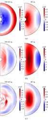Fig. 21. Similar to Fig. 16 but for the 1g mode. Non-axisymmetric (left) and axisymmetric (right) toroidal velocity uϕ of the 1g mode for Ωs = 100/π Hz and Ct = 1.36 × 10−3 (Panel a), for Ωs = 100 Hz and Ct = 5.3 × 10−3 (Panel b) and for Ωs = 0 with a tidal amplitude of Ct = 5.3 × 10−3 (Panel c).

We can confirm spin-up in the inner region for all three cases by looking at the axisymmetric toroidal velocity u_ϕ in the meridional plane (right panels of Fig. 21). First, we see similar effects of rotation and increased tidal amplitude than for the ₂g mode: when modes become more nonlinear (increased tidal amplitude and/or reduced rotation), the axisymmetric component becomes stronger compared to the non-axisymmetric component and clearly dominates for the nonrotating case with increased amplitude. The impact of rotation is also clearly seen as the flow with Ω_s = 100 Hz is more cylindrical than the other cases, whereas the spherical geometry of gravity dominates in the two other cases. The geometry for the non-axisymmetric components is different as there is only one radial wavelength and there are more structures close to the inner core. The axisymmetric component also seems to be shifted toward the interior compared to the ₂g mode (Fig. 16). By comparing the right panels of Figs. 16 and 21, we see that the axisymmetric toroidal velocity is stronger for the ₁g mode in the rotating cases, which may be due to the increased tidal amplitude and also that the ₁g mode resonance is stronger even for a similar tidal amplitude (see Sect. 2.2.2).

To confirm that the inner spin-up is stronger for this simulation, we estimated the spin-up in the first half of the shell as in Eq. (36). We find that Ω_s, end ∈ [17.3 Hz, 1.1Ω_s, 1.18Ω_s] for an initial Ω_s ∈ [0, 100/π, 100] Hz. This is consistent with the fact that the axisymmetric azimuthal velocities are stronger for the ₁g mode in rotating cases.

5.2.3. Implications for dynamo activity and gravitational waves

We find that the kinetic energy of the tidally excited flow would be enough to generate a magnetic field of > 10¹⁴ G assuming equipartition for the ₂g mode and > 10¹⁵ G for the ₁g mode. However, the bulk of this energy will likely be localized to small scales, and it is unclear if the corresponding dipole growth would be enough to explain precursor luminosities. Under the assumption of an incompressible fluid and the smooth BV frequency shown in Fig. 11, the modes are localized closer to the core than to the crust and would most likely generate the magnetic field there. However, from linear calculations with a realistic NS profile with the APR4 EOS, the mode velocity is faster in the crust, so we can expect (in principle) to have the differential rotation in the crust, where it would amplify the magnetic field that is most relevant for electromagnetic observables. If we assume that the strength of the dipole is 5% of the total magnetic field, as found in simulations of the magnetorotational instabilities (Reboul-Salze et al. 2021, 2022), it may be enough to explain the luminosity of precursors (Suvorov et al. 2024b). This needs to be further studied in simulations with magnetic transport included and compared with a more realistic interior, which is out of the scope of this paper. Still, the results are promising.

We also find that the star, for ₂g and ₁g modes and for all rotation rates, would get spin-up by the resonance. This implies that we can expect the tidal forcing frequency $\widehat{\omega }=2({\mathrm{\Omega }}_o-{\mathrm{\Omega }}_s)$ to remain in the resonance window longer as the orbital frequency Ω_o evolves due to the emission of GWs. This depends on the size of the window but roughly lies in the range $0.99{\omega }_{\mathrm{resonnant}}\le \widehat{\omega }\le 1.01{\omega }_{\mathrm{resonnant}}$, so that a spin-up of 10% would increase the resonant window timescale by a factor ∼5. This phenomenon, known as tidal resonance locking with gravity or inertial modes, has been studied in such various contexts as massive and dwarf stellar binary systems, Jovian and Saturnian systems, and short-period exoplanetary systems (e.g., Witte & Savonije 1999; Burkart et al. 2013; Fuller et al. 2016; Ma & Fuller 2021, respectively). The above estimate is made by assuming that the loss of orbital energy due to the growth of the gravito-inertial modes and the spin-up can be neglected compared to the emission of GWs. Otherwise, the inspiral rate could be faster, compensating for the growth of the resonance window. The full orbital evolution problem needs to be solved to understand the system’s response, which is left to future studies.

6. Discussions

6.1. Consequences for BH-NS mergers

The calculations done in this study are practically independent of the details of body 2. We could therefore extrapolate our results to cases relevant for a black hole with M₂ > M₁. This means that the tidal amplitude parameter, $ϵ=\frac{M_2}{M_1}{\left(\frac{R_o}{a}\right)}^3$, would increase for a given semimajor axis a. This may lead to stronger tidal amplitudes; in particular, for a given orbital frequency Ω_o corresponding to a resonant frequency, the tidal amplitude parameter ϵ can be written as $ϵ=\frac{M_2}{M_1+M_2}{\left(\frac{{\mathrm{\Omega }}_o}{{\omega }_d}\right)}^2$ by using $a^3=\frac{G(M_1+M_2)}{{\mathrm{\Omega }}_o^2}$ and $R_o^3=\frac{G{M}_1}{{\omega }_d^2}$, which would increase by a maximum factor of ∼2. Stronger nonlinear effects are therefore expected, provided the resonance occurs, most likely without changing qualitatively the results of this study.

6.2. Interior structure

Comparison between results from Sects. 4 and 5 shows the importance of the NS interior model. Indeed, the BV frequency in Sect. 5 is higher by a factor of ≈2 − 5 from the inner to the outer boundaries. This increase in the BV frequency leads to stronger nonlinear effects. As the BV frequency is strongly dependent on the internal microphysics, a change in the NS model could impact the conclusions of this study. Additionally, the tidal amplitude parameter is dependent on the NS radius R_o and an increase in 20% in this quantity for a different EOS at a fixed mass would lead to an increase in ≈1.7 in the amplitude of a given mode, which may then change the nonlinear saturation (see also Suvorov et al. 2024a). The density profile also changes with the EOS, which would further impact the mode eigenfunctions. Density profiles can be taken into account with an anelastic model, the development of which is left to future studies owing to numerical challenges: the density gradient has to be taken into account in the computation of the equilibrium tides. This would be especially important in studying the resonant modes in the crust, where proposed late-stage amplifications of near-surface magnetic fields have been invoked to explain the luminosity of GRB precursors as the Ohmic decay timescale is expected to be much shorter than the orbital lifetime (e.g., Pons & Viganò 2019).

6.3. Formulation issues

As with most numerical studies of astrophysical phenomena, some limitations are inevitable as physical time- and length-scales typically span many orders of magnitude in such systems. Indeed, the formulation presented in this article has a few limitations, which we highlight here and in the sections below for completeness.

(i) The formulation cannot reproduce f-mode resonances or g-mode resonances too close to the f-mode frequency as this mode is “hard coded” in the static tide (the Love number in the equilibrium velocity). Moreover, a fixed surface does not capture f-mode oscillations (Pontin et al. 2023). (ii) In the nonresonant regime, the formulation cannot reproduce results with a free surface. This can be corrected by changing the stress-free boundary conditions to match the free surface case. However, its implementation with the scalar potentials in the nonlinear code can be difficult or may lead to unexpected effects and the study of the regime, away from the BV frequency, is left to further studies. (iii) The use of a spherical shell leads to the neglect of nonlinear interactions between the equilibrium and dynamical tides. It can be justified by some physical scaling arguments (see Astoul & Barker 2022) but when the resonant modes occupy the largest scales, these nonlinear interactions might become relevant.

6.4. Cowling approximation

A simplifying hypothesis employed throughout is the Cowling approximation, the neglect of equilibrium and dynamical perturbations to the background gravitational potential ∇Φ_g = g. These effects could have a strong impact on the amplitude of the modes; however, the linear study of Xu & Lai (2017) found a reduction down to 20% of the initial amplitude in cases without perturbations to the self-gravity potential. Nonetheless, it is unknown how the dynamical perturbations to self-gravity ${\mathrm{\Phi }}_g\prime$ in our setup, where we assumed a constant density, would impact the modes and their nonlinear saturation. In addition, neglecting the equilibrium perturbations to self-gravity Φ_g^e removes a term ∝(1 + k₂) in the amplitude of the equilibrium tide, where k₂ is the Love number associated with the ℓ = 2 tide. For NSs, realistic calculations of Love numbers give k₂ ≳ 0.1 (Flanagan & Hinderer 2008; Hinderer 2008; Hinderer et al. 2010), meaning we underestimate the amplitude by ≳10%. Overall, we seem to neglect both positive and negative effects of the self-gravity and the impact of this assumption needs to be further studied as it could be exacerbated to some degree for a realistic stellar density profile.

6.5. Dissipation processes

The simulations presented in this work have been carried out with unrealistic viscosities and thermal and/or compositional diffusivities that could change the results. For example, in a NS, the microphysical viscosities are estimated to be at least 10 orders of magnitude lower than those used here. For the thermal and/or composition diffusivities, the value depends highly on the NS model and evolutionary pathway (e.g., whether there was a history of recycling; see Suvorov et al. 2024a). In linear studies, such as Pontin et al. (2023, 2024), it has been found that decreasing the viscosity/thermal diffusivity by ∼2 orders of magnitude leads to a comparable increase in the total (frequency-dependent) tidal dissipation and mode kinetic energy. On a positive note, this suggests that the mode amplitudes found in this study can be seen as lower limits and may be larger in astrophysical circumstances. This also means that nonlinear effects are more relevant, especially with respect to how saturation depends on damping processes. It is for this reason that we chose to study the nonrotating case with an increased tidal frequency. However, triadic resonances, corotation resonances, or other secondary instabilities (such as shear-flow instabilities) may lead to a different saturation mechanism that is largely insensitive to the viscosity and thermal diffusivity below some critical values. Studying the impact of viscosity and thermal diffusivity is required to understand the nonlinear saturation and to explore a wider range of parameters; this will be the subject of future work.

Moreover, the resonant peaks (see, e.g., Fig. 1) may also become narrower and the relevant resonant window itself could become smaller. A study that takes into account the evolution of the tidal forcing frequency and tidal amplitude due to the emission of GWs would be required to see whether the modes are able to draw enough energy from the time-varying orbit and reach a similar amplitude as the modes presented in this study.

7. Conclusions and perspectives

In this article, a new formulation, building on that of Astoul & Barker (2022, 2023) but applied here to a stably stratified instead of neutrally stratified region, was derived in order to simulate the nonlinear saturation of gravito-inertial modes in a self-consistent manner that separates equilibrium and dynamical tides. To ensure consistency with previous formulations applied to a stably stratified model that do not distinguish between dynamical and equilibrium tides, we first tested the linear limit of this scheme and find excellent agreement with previous studies for both pure and gravito-inertial modes, provided the tidal forcing frequency is not so high as to approach the f- or acoustic-mode frequencies (Sect. 3), where nonlinear effects may be important in any case (Kuan et al. 2025).

The nonlinear code was benchmarked against the linear results in Sect. 3 with a uniform entropy and/or composition gradient, yielding again quantitative agreement in the expected regimes of validity. With a homogeneous BV frequency of N = 0.045ω_d and a dimensionless tidal amplitude of C_t ∼ 10⁻³, such a comparison demonstrates the impact of nonlinear effects for several modes in the form of a generated, axisymmetric kinetic energy representing ≳5% of the total kinetic energy. As seen in Sect. 4, we find in particular that the strongest resonant modes are indeed able to generate kinetic energy representing order 10% of the total kinetic energy. This axisymmetric component is dominated by the toroidal velocity, u_ϕ, which is optimistic from the perspective of enticing premerger dynamo activity and the generation of magnetic fields, as first suggested by Suvorov et al. (2024a).

Although the formalism is general, it has been primarily applied in the context of neutron-star binaries in this work; astrophysical applications for gravito-inertial modes were considered in Sect. 5. A BV profile based on Tolman–Oppenheimer–Volkoff equations calculations with the APR4+DH EOS, smoothed out in the crust, was considered in an effort to consider realistic profiles even though the formalism here is strictly Newtonian; such hybrid schemes are common in the literature, especially because a fully relativistic treatment of tides is difficult (see Suvorov et al. 2024a, for a discussion). Comparisons with the GR linear calculations demonstrate quantitative agreement for pure g-modes in the stellar core but not in the crust (see Fig. 12). This is primarily due to the impact of the radially varying density profile and compositional discontinuities in the crust, which we neglect via the Boussinesq approximation. The linear code was then used to compute the resonant frequencies to study the nonlinear saturation at the frequencies of the ₁g and ₂g modes. We find that with a stronger BV frequency compared to Sect. 4, nonlinear effects dominate even more in determining the saturation of the modes. Remarkably, the axisymmetric kinetic energy can constitute up to 95% of the total mode energy. Overall, we argue that if the kinetic energy were efficiently converted into magnetic energy, a magnetic field of 10¹⁴ − 10¹⁵ G could be generated. If this occurs via the MRI, appealing to previous studies that quantified multipolar energy distributions (Reboul-Salze et al. 2021, 2022) suggests the anticipated strength of the dipole component would be between 5 × 10¹² − 5 × 10¹³ G. This would be enough to explain the luminosity of (at least most) precursors (e.g., Tsang et al. 2012; Xiao et al. 2024).

We also find that the NS should get spun-up by resonances as u_ϕ is non-negligible (e.g., Fig. 16). The rotation rate in the inner half of the domain may be increased by up to ∼10% for already-rotating cases and up to ∼20 Hz in the nonrotating case. Such an increase would lead to the tidal forcing frequency of $\widehat{\omega }=2({\mathrm{\Omega }}_o-{\mathrm{\Omega }}_s)$ remaining in the resonance window for longer as the orbital frequency, Ω_o, sweeps up due to the emission of GWs. Linear studies of gravito-inertial modes in NSs may therefore underestimate the amplitude of these modes as this lengthening, and hence the duration of energy transfer, has not been considered. Stronger saturation should therefore be studied in more detail as it could lead to a greater degree of dephasing and make a more optimistic case for the detectability of dynamical tides with next-generation GW interferometers (Ho & Andersson 2023).

Acknowledgments

Linear simulations were run on the Yamazaki cluster at the Max-Planck Institute for Gravitational Physics, Potsdam. nonlinear simulations were run on the Sakura cluster at the Max Planck Computing and Data Facility (MPCDF) in Garching, Germany. AGS is grateful for support provided by the Conselleria d’Educació, Cultura, Universitats i Ocupació de la Generalitat Valenciana through Prometeo Project CIPROM/2022/13. AA has been funded by a Leverhulme Trust Early Career Fellowship (ECF-2022-362). The authors thank A. Barker for helpful discussions about the treatment of tides, and more specifically the validity of different dynamical/equilibrium tide decompositions.

References

All Figures

	Fig. 1. Kinetic energy as a function of the tidal frequency, $\widehat{\omega }$, depending on the formulation used (see plot legends). Crosses correspond to the g-mode frequencies in a cavity (Eq. (B9) of Pontin et al. 2023). Code units are used such that Ro = 1, ωd = 1, and ρ0 = 1.
In the text

	Fig. 2. Comparison of the toroidal velocity uϕ for resonant modes in the full formulation (Panel a) and the split formulation (Panel b) for two representative tidal frequencies $\widehat{\omega }=0.1$ (left) and $\widehat{\omega }=1.56$ (right).
In the text

Fig. 3. Kinetic energies of tidally excited fluid motions as functions of the tidal forcing frequency, $\widehat{\omega }$, when the full tidal potential is taken into account (blue) and when the tidal forcing is effectively described using the equilibrium tidal flow (orange). The dashed orange line also corresponds to the split formulation but with different boundary conditions (see text), while the solid green line corresponds to the modes obtained only with the effective tidal forcing, ft, due to Coriolis force. Pure g-modes frequencies (black, Eq. (33)) and negative g-modes (red) are designated by a cross. A Rossby mode resonance is highlighted at $\widehat{\omega }=-0.9{\mathrm{\Omega }}_s/3$.

In the text

Fig. 4. Comparison of two gravito-inertial modes along ϕ = 0 for the different formulations. The first mode, with $\widehat{\omega }=0.421N$, corresponds to the 1g22 mode impacted by the rotation, while the second one is closer to an inertial or gravito-inertial mode, $\widehat{\omega }=0.777N$. Velocities are given in units such that Roωd = 1.56 × 1010 cm s−1. Left: Toroidal velocity uϕ at ϕ = 0 for $\widehat{\omega }=0.421N$ in the full formulation (Panel a), split formulation (Panel b) and with only effective Coriolis forcing (Panel c). Right: Toroidal velocity uϕ at ϕ = 0 for $\widehat{\omega }=0.777N$ in the full formulation (Panel a), split formulation (Panel b) and with only effective Coriolis forcing (Panel c).

In the text

	Fig. 5. Toroidal velocity, uϕ, with $\widehat{\omega }=0.777N$ in the full formulation (left), and in the split formulation (right) with modified non stress-free boundary conditions (see text).
In the text

	Fig. 6. Power and dissipation balance of the tidally excited fluid motions as a function of the tidal forcing frequency, $\widehat{\omega }$, with the split formulation of the tidal forcing with N/Ωs = 3.24. Similar to Fig. 3, the pure g-mode frequency (Eq. (33)) is designated by crosses.
In the text

	Fig. 7. Kinetic energy along the tidal frequency, $\widehat{\omega }$, for the linear code (dashed lines) or the nonlinear simulations (scatter points) with Ct = 10−3. The color scale of the nonlinear simulations corresponds to the ratio of the axisymmetric kinetic to the total kinetic energy.
In the text

	Fig. 8. 3g-mode resonance with $\widehat{\omega }=0.126N$ at ϕ = 0 in the case of small rotation (N/Ωs = 3.24). Results of the linear code are shown on the left, while that of the nonlinear code are on the right; notice the difference in the color bar for each panel.
In the text

	Fig. 9. Time evolution of the kinetic energy for the nonlinear simulations of 1g and 2g modes compared to the linear results (dashed red lines). The lines above correspond to the 1g mode with $\widehat{\omega }=0.348N$. The lines below correspond to the 2g− mode with $\widehat{\omega }=0.186N$, which are rescaled by a factor of 0.1 for improved visibility.
In the text

	Fig. 10. Strongest two g-mode resonances and their nonlinear saturation in the case of small rotation (N/Ωs = 3.24). Non-axisymmetric (left) and axisymmetric (right) toroidal velocity uϕ for the 2g mode (Panel a) and for the 1g mode (Panel b).
In the text

	Fig. 11. BV frequency for a 1.6 M⊙ NS with the APR4 EOS, giving a radius of Ro = 11 km from Suvorov et al. (2024a). The orange line is the profile that is used in the Newtonian simulations presented here (see main text for details). For reference, we overlay the BV frequency of the setup in Sect. 4 (dashed line).
In the text

	Fig. 12. Toroidal velocity for 1g22 and 2g22 modes. Solid lines represent the cases as those in Fig. 1 of Suvorov et al. (2024a).
In the text

	Fig. 13. Time evolution of the kinetic energy for the 2g mode for Ωs = 100/π Hz, (top), Ωs = 100 Hz (middle), and Ωs = 0 with an increased tidal amplitude (bottom).
In the text

Fig. 14. Kinetic energy spectra of the 2g-mode resonance for Ωs = 100/π Hz, (top), Ωs = 100 Hz (middle), and Ωs = 0 with an increased tidal amplitude (bottom). The left panels denote kinetic energy integrated over r and m, while varying ℓ; and the right panels are integrated over r and ℓ, while varying m. The kinetic energy is in viscous units. The tidal amplitude is Ct = 9.3 × 10−4 in Panel a, Ct = 4.1 × 10−3 in Panel b and in Panel c.

In the text

	Fig. 15. Velocity flows (in CGS units), ur (left) and uϕ (right), of the gravito-inertial 2g mode in the equatorial plane for Ωs = 100/π Hz (top), Ωs = 100 Hz (middle), and Ωs = 0 with an increased tidal amplitude (bottom). The tidal amplitude is Ct = 9.3 × 10−4 in Panel a, Ct = 4.1 × 10−3 in Panel b and in Panel c.
In the text

Fig. 16. Velocity flow (in CGS units) of the gravito-inertial 2g mode in the meridional plane for Ωs = 100/π Hz, (top), Ωs = 100 Hz (middle), and Ωs = 0 with an increased tidal amplitude (bottom). Non-axisymmetric (left) and axisymmetric (right) toroidal velocity uϕ of the 2g mode for Ωs = 100/π Hz and Ct = 9.3 × 10−4 (Panel a), for Ωs = 100 Hz and Ct = 4.1 × 10−3 (Panel b) and for Ωs = 0 with a tidal amplitude of Ct = 4.1 × 10−3 (Panel c).

In the text

	Fig. 17. Time evolution of the kinetic energy for the 1g mode for Ωs = 100/π Hz (top), Ωs = 100 Hz (middle), and Ωs = 0 with an increased tidal amplitude of Ct = 5.3 × 10−3 (bottom).
In the text

	Fig. 18. Similar to Fig. 14 but for the 1g-mode. We compare the spectrum to several wave scaling laws corresponding to ℓ−5/3, ℓ−2, and ℓ−3 (dotted lines) from internal wave turbulence (Le Reun et al. 2018, 2020). The tidal amplitude is Ct = 1.36 × 10−3 in Panel a and Ct = 5.3 × 10−3 in Panel b and Panel c.
In the text

Fig. 19. Fourier transform of the poloidal velocity potential, W, showing the different main modes for Ωs = 100/π Hz (top), Ωs = 100 Hz (middle), and Ωs = 0 (bottom). We obtain ω1 ∈ [63.1, 58.2, 73.7] Hz and ${\omega }_2=\widehat{\omega }-{\omega }_1$. In the nonrotating case, the FFT in the first phase, t ∈ [0, 4] s, is plotted with the dotted line, while the second phase, t ∈ [4, 10] s, is plotted with solid lines.

In the text

	Fig. 20. Similar to Fig. 15 but for 1g modes. The tidal amplitude is Ct = 1.36 × 10−3 in Panel a and Ct = 5.3 × 10−3 in Panel b and Panel c.
In the text

	Fig. 21. Similar to Fig. 16 but for the 1g mode. Non-axisymmetric (left) and axisymmetric (right) toroidal velocity uϕ of the 1g mode for Ωs = 100/π Hz and Ct = 1.36 × 10−3 (Panel a), for Ωs = 100 Hz and Ct = 5.3 × 10−3 (Panel b) and for Ωs = 0 with a tidal amplitude of Ct = 5.3 × 10−3 (Panel c).
In the text

References

- Aerts, C., & Tkachenko, A. 2024, A&A, 692, R1 [NASA ADS] [CrossRef] [EDP Sciences] [Google Scholar]
- Aerts, C., Christensen-Dalsgaard, J., & Kurtz, D. W. 2010, Asteroseismology (Springer Science+Business Media B.V.) [Google Scholar]
- Akmal, A., Pandharipande, V. R., & Ravenhall, D. G. 1998, Phys. Rev. C, 58, 1804 [Google Scholar]
- Alexander, M. E. 1987, MNRAS, 227, 843 [NASA ADS] [CrossRef] [Google Scholar]
- Andersson, N., & Pnigouras, P. 2020, Phys. Rev. D, 101, 083001 [Google Scholar]
- Astoul, A., & Barker, A. J. 2022, MNRAS, 516, 2913 [NASA ADS] [CrossRef] [Google Scholar]
- Astoul, A., & Barker, A. J. 2023, ApJ, 955, L23 [NASA ADS] [CrossRef] [Google Scholar]
- Astoul, A., & Barker, A. J. 2025, MNRAS, 541, 1575 [Google Scholar]
- Baiko, D. A. 2024, MNRAS, 528, 408 [Google Scholar]
- Baiko, D. A., & Chugunov, A. I. 2018, MNRAS, 480, 5511 [NASA ADS] [CrossRef] [Google Scholar]
- Balbus, S. A., & Hawley, J. F. 1998, Rev. Mod. Phys., 70, 1 [Google Scholar]
- Barik, A., Triana, S. A., Hoff, M., & Wicht, J. 2018, J. Fluid Mech., 843, 211 [Google Scholar]
- Barik, A., Triana, S. A., Hoff, M., & Wicht, J. 2024, J. Fluid Mech., 1001, A1 [Google Scholar]
- Barker, A. J. 2011, MNRAS, 414, 1365 [Google Scholar]
- Barker, A. J. 2016, MNRAS, 459, 939 [Google Scholar]
- Barker, A. J. 2022, ApJ, 927, L36 [NASA ADS] [CrossRef] [Google Scholar]
- Barker, A. J., & Ogilvie, G. I. 2010, MNRAS, 404, 1849 [NASA ADS] [Google Scholar]
- Barker, A. J., & Ogilvie, G. I. 2011, MNRAS, 417, 745 [CrossRef] [Google Scholar]
- Bellet, F., Godeferd, F. S., Scott, J. F., & Cambon, C. 2006, J. Fluid Mech., 562, 83 [Google Scholar]
- Bolmont, E., & Mathis, S. 2016, Celest. Mech. Dyn. Astron., 126, 275 [Google Scholar]
- Burkart, J., Quataert, E., Arras, P., & Weinberg, N. N. 2013, MNRAS, 433, 332 [NASA ADS] [CrossRef] [Google Scholar]
- Burns, K. J., Vasil, G. M., Oishi, J. S., Lecoanet, D., & Brown, B. P. 2020, Phys. Rev. Res., 2, 023068 [NASA ADS] [CrossRef] [Google Scholar]
- Christensen, U., & Wicht, J. 2015, Treatise on Geophysics, 2nd edn. (Oxford: Elsevier), 245 [Google Scholar]
- Ciolfi, R. 2020, Gen. Relat. Grav., 52, 59 [Google Scholar]
- Coppin, P., de Vries, K. D., & van Eijndhoven, N. 2020, Phys. Rev. D, 102, 103014 [Google Scholar]
- Counselman, C. C., III 1973, ApJ, 180, 307 [NASA ADS] [CrossRef] [Google Scholar]
- Couston, L.-A., Lecoanet, D., Favier, B., & Le Bars, M. 2018, Phys. Rev. Lett., 120, 244505 [Google Scholar]
- Damour, T., & Nagar, A. 2009, Phys. Rev. D, 80, 084035 [NASA ADS] [CrossRef] [Google Scholar]
- Dewberry, J. W. 2023, MNRAS, 521, 5991 [NASA ADS] [CrossRef] [Google Scholar]
- Dhouib, H., Baruteau, C., Mathis, S., et al. 2024, A&A, 682, A85 [NASA ADS] [CrossRef] [EDP Sciences] [Google Scholar]
- Dintrans, B., & Rieutord, M. 2000, A&A, 354, 86 [NASA ADS] [Google Scholar]
- Dintrans, B., Rieutord, M., & Valdettaro, L. 1999, J. Fluid Mech., 398, 271 [Google Scholar]
- Douchin, F., & Haensel, P. 2001, A&A, 380, 151 [NASA ADS] [CrossRef] [EDP Sciences] [Google Scholar]
- Duchêne, G., & Kraus, A. 2013, ARA&A, 51, 269 [Google Scholar]
- El-Badry, K. 2024, New Astron. Rev., 98, 101694 [NASA ADS] [CrossRef] [Google Scholar]
- Essick, R., & Weinberg, N. N. 2016, ApJ, 816, 18 [Google Scholar]
- Favier, B., Barker, A. J., Baruteau, C., & Ogilvie, G. I. 2014, MNRAS, 439, 845 [Google Scholar]
- Flanagan, É. É., & Hinderer, T. 2008, Phys. Rev. D, 77, 021502 [NASA ADS] [CrossRef] [Google Scholar]
- Fuller, J., Luan, J., & Quataert, E. 2016, MNRAS, 458, 3867 [Google Scholar]
- Fuller, J., Guillot, T., Mathis, S., & Murray, C. 2024, Space Sci. Rev., 220, 22 [CrossRef] [Google Scholar]
- Galtier, S. 2003, Phys. Rev. E, 68, 015301 [Google Scholar]
- Gastine, T., & Wicht, J. 2012, Icarus, 219, 428 [Google Scholar]
- Gilman, P. A., & Glatzmaier, G. A. 1981, ApJS, 45, 335 [CrossRef] [Google Scholar]
- Goldreich, P., & Nicholson, P. D. 1989, ApJ, 342, 1079 [Google Scholar]
- Guo, Z., Ogilvie, G. I., & Barker, A. J. 2023, MNRAS, 521, 1353 [Google Scholar]
- Hegade, K. R. A., Ripley, J. L., & Yunes, N., 2024, Phys. Rev. D, 109, 104064 [Google Scholar]
- Hinderer, T. 2008, ApJ, 677, 1216 [NASA ADS] [CrossRef] [Google Scholar]
- Hinderer, T., Lackey, B. D., Lang, R. N., & Read, J. S. 2010, Phys. Rev. D, 81, 123016 [NASA ADS] [CrossRef] [Google Scholar]
- Hinderer, T., Taracchini, A., Foucart, F., et al. 2016, Phys. Rev. Lett., 116, 181101 [Google Scholar]
- Ho, W. C. G., & Andersson, N. 2023, Phys. Rev. D, 108, 043003 [Google Scholar]
- Jackson, B., Greenberg, R., & Barnes, R. 2008, ApJ, 678, 1396 [Google Scholar]
- Ji, S., Fuller, J., & Lecoanet, D. 2023, MNRAS, 521, 5372 [NASA ADS] [CrossRef] [Google Scholar]
- Kerswell, R. R. 1999, J. Fluid Mech., 382, 283 [Google Scholar]
- Kokkotas, K. D., & Schafer, G. 1995, MNRAS, 275, 301 [NASA ADS] [CrossRef] [Google Scholar]
- Kuan, H.-J., Suvorov, A. G., & Kokkotas, K. D. 2021a, MNRAS, 506, 2985 [NASA ADS] [CrossRef] [Google Scholar]
- Kuan, H.-J., Suvorov, A. G., & Kokkotas, K. D. 2021b, MNRAS, 508, 1732 [NASA ADS] [CrossRef] [Google Scholar]
- Kuan, H.-J., Suvorov, A. G., & Kokkotas, K. D. 2023, A&A, 676, A59 [NASA ADS] [CrossRef] [EDP Sciences] [Google Scholar]
- Kuan, H.-J., Kiuchi, K., & Shibata, M. 2025, Phys. Rev. Lett., 135, 141403 [Google Scholar]
- Kwon, K. J., Yu, H., & Venumadhav, T. 2024, arXiv e-prints [arXiv:2410.03831] [Google Scholar]
- Kwon, K. J., Yu, H., & Venumadhav, T. 2025, arXiv e-prints [arXiv:2503.11837] [Google Scholar]
- Lai, D., & Wu, Y. 2006, Phys. Rev. D, 74, 024007 [NASA ADS] [CrossRef] [Google Scholar]
- Lazovik, Y. A., Barker, A. J., de Vries, N. B., & Astoul, A. 2024, MNRAS, 527, 8245 [Google Scholar]
- Le Reun, T., Favier, B., & Le Bars, M. 2018, J. Fluid Mech., 840, 498 [Google Scholar]
- Le Reun, T., Favier, B., & Le Bars, M. 2020, EPL, 132, 64002 [Google Scholar]
- Lecoanet, D., Vasil, G. M., Fuller, J., Cantiello, M., & Burns, K. J. 2017, MNRAS, 466, 2181 [Google Scholar]
- Lin, Y. 2023, A&A, 671, A37 [NASA ADS] [CrossRef] [EDP Sciences] [Google Scholar]
- Lin, Y., & Ogilvie, G. I. 2018, MNRAS, 474, 1644 [Google Scholar]
- Ma, L., & Fuller, J. 2021, ApJ, 918, 16 [NASA ADS] [CrossRef] [Google Scholar]
- Mathis, S. 2009, A&A, 506, 811 [CrossRef] [EDP Sciences] [Google Scholar]
- Ogilvie, G. I. 2009, MNRAS, 396, 794 [Google Scholar]
- Ogilvie, G. I. 2013, MNRAS, 429, 613 [Google Scholar]
- Ogilvie, G. I. 2014, ARA&A, 52, 171 [Google Scholar]
- Ogilvie, G. I., & Lin, D. N. C. 2004, ApJ, 610, 477 [Google Scholar]
- Passamonti, A., Andersson, N., & Pnigouras, P. 2021, MNRAS, 504, 1273 [NASA ADS] [CrossRef] [Google Scholar]
- Peters, P. C. 1964, Phys. Rev., 136, 1224 [Google Scholar]
- Pitre, T., & Poisson, E. 2025, arXiv e-prints [arXiv:2506.08722] [Google Scholar]
- Pnigouras, P., & Kokkotas, K. D. 2015, Phys. Rev. D, 92, 084018 [Google Scholar]
- Pons, J. A., & Viganò, D. 2019, Liv. Rev. Comput. Astrophys., 5, 3 [Google Scholar]
- Pontin, C. M., Barker, A. J., & Hollerbach, R. 2023, ApJ, 950, 176 [NASA ADS] [CrossRef] [Google Scholar]
- Pontin, C. M., Barker, A. J., & Hollerbach, R. 2024, ApJ, 960, 32 [NASA ADS] [CrossRef] [Google Scholar]
- Press, W. H., & Teukolsky, S. A. 1977, ApJ, 213, 183 [NASA ADS] [CrossRef] [Google Scholar]
- Reboul-Salze, A., Guilet, J., Raynaud, R., & Bugli, M. 2021, A&A, 645, A109 [NASA ADS] [CrossRef] [EDP Sciences] [Google Scholar]
- Reboul-Salze, A., Guilet, J., Raynaud, R., & Bugli, M. 2022, A&A, 667, A94 [NASA ADS] [CrossRef] [EDP Sciences] [Google Scholar]
- Rieutord, M. 2009, Lect. Notes Phys., 765, 101 [Google Scholar]
- Schaeffer, N. 2013, Geochem. Geophys. Geosyst., 14, 751 [NASA ADS] [CrossRef] [Google Scholar]
- Semin, B., Facchini, G., Pétrélis, F., & Fauve, S. 2016, Phys. Fluids, 28, 096601 [Google Scholar]
- Spiegel, E. A., & Veronis, G. 1960, ApJ, 131, 442 [NASA ADS] [CrossRef] [Google Scholar]
- Stewartson, K. 1966, J. Fluid Mech., 26, 131 [NASA ADS] [CrossRef] [Google Scholar]
- Suvorov, A. G., & Kokkotas, K. D. 2020, Phys. Rev. D, 101, 083002 [NASA ADS] [CrossRef] [Google Scholar]
- Suvorov, A. G., Kuan, H. J., & Kokkotas, K. D. 2022, A&A, 664, A177 [NASA ADS] [CrossRef] [EDP Sciences] [Google Scholar]
- Suvorov, A. G., Kuan, H.-J., Reboul-Salze, A., & Kokkotas, K. D. 2024a, Phys. Rev. D, 109, 103023 [Google Scholar]
- Suvorov, A. G., Kuan, H.-J., & Kokkotas, K. D. 2024b, Universe, 10, 441 [Google Scholar]
- Taniguchi, K., & Shibata, M. 2010, ApJS, 188, 187 [Google Scholar]
- Thompson, C., & Duncan, R. C. 1993, ApJ, 408, 194 [NASA ADS] [CrossRef] [Google Scholar]
- Tilgner, A., & Busse, F. H. 1997, J. Fluid Mech., 332, 359 [NASA ADS] [CrossRef] [Google Scholar]
- Tsang, D., Read, J. S., Hinderer, T., Piro, A. L., & Bondarescu, R. 2012, Phys. Rev. Lett., 108, 011102 [NASA ADS] [CrossRef] [Google Scholar]
- Wang, J.-S., Peng, Z.-K., Zou, J.-H., Zhang, B.-B., & Zhang, B. 2020, ApJ, 902, L42 [NASA ADS] [CrossRef] [Google Scholar]
- Weinberg, N. N., Arras, P., Quataert, E., & Burkart, J. 2012, ApJ, 751, 136 [NASA ADS] [CrossRef] [Google Scholar]
- Weinberg, N. N., Arras, P., & Burkart, J. 2013, ApJ, 769, 121 [NASA ADS] [CrossRef] [Google Scholar]
- Weinberg, N. N., Davachi, N., Essick, R., et al. 2024, ApJ, 960, 50 [NASA ADS] [CrossRef] [Google Scholar]
- Wicht, J. 2002, Phys. Earth Planet. Inter., 132, 281 [Google Scholar]
- Witte, M. G., & Savonije, G. J. 1999, A&A, 350, 129 [NASA ADS] [Google Scholar]
- Xiao, S., Zhang, Y.-Q., Zhu, Z.-P., et al. 2024, ApJ, 970, 6 [Google Scholar]
- Xu, W., & Lai, D. 2017, Phys. Rev. D, 96, 083005 [NASA ADS] [CrossRef] [Google Scholar]
- Yu, H., Weinberg, N. N., Arras, P., Kwon, J., & Venumadhav, T. 2023, MNRAS, 519, 4325 [NASA ADS] [CrossRef] [Google Scholar]
- Yu, H., Arras, P., & Weinberg, N. N. 2024, Phys. Rev. D, 110, 024039 [Google Scholar]
- Zahn, J. P. 1966, Ann. Astrophys., 29, 489 [NASA ADS] [Google Scholar]
- Zahn, J.-P. 2013, Lect. Notes Phys., 861, 301 [NASA ADS] [CrossRef] [Google Scholar]
- Zhou, Y., & Zhang, F. 2017, ApJ, 849, 114 [Google Scholar]