| Issue |
A&A
Volume 704, December 2025
|
|
|---|---|---|
| Article Number | A110 | |
| Number of page(s) | 28 | |
| Section | Cosmology (including clusters of galaxies) | |
| DOI | https://doi.org/10.1051/0004-6361/202554942 | |
| Published online | 05 December 2025 | |
The SRG/eROSITA All-Sky Survey
The weak-lensing mass calibration and the stellar mass-to-halo mass relation from the Hyper Suprime-Cam Subaru Strategic Program
1
Department of Physics, National Cheng Kung University, No.1, University Road, Tainan City 70101, Taiwan
2
Max Planck Institute for Extraterrestrial Physics, Giessenbachstrasse 1, 85748 Garching, Germany
3
INAF, Osservatorio di Astrofisica e Scienza dello Spazio, Via Piero Gobetti 93/3, I-40129 Bologna, Italy
4
Universität Innsbruck, Institut für Astro- und Teilchenphysik, Technikerstr. 25/8, 6020 Innsbruck, Austria
5
Physics Program, Graduate School of Advanced Science and Engineering, Hiroshima University, 1-3-1 Kagamiyama, Higashi-Hiroshima, Hiroshima 739-8526, Japan
6
Hiroshima Astrophysical Science Center, Hiroshima University, 1-3-1 Kagamiyama, Higashi-Hiroshima, Hiroshima 739-8526, Japan
7
Core Research for Energetic Universe, Hiroshima University, 1-3-1, Kagamiyama, Higashi-Hiroshima, Hiroshima 739-8526, Japan
8
IRAP, Université de Toulouse, CNRS, UPS, CNES, Toulouse, France
9
Institute of Astronomy and Astrophysics, Academia Sinica, P.O. Box 23-141 Taipei 10617, Taiwan
10
Center for Frontier Science, Chiba University, 1-33 Yayoi-cho, Inage-ku, Chiba 263-8522, Japan
11
Department of Physics, Graduate School of Science, Chiba University, 1-33 Yayoi-Cho, Inage-Ku, Chiba 263-8522, Japan
12
Argelander-Institut für Astronomie (AIfA), Universität Bonn, Auf dem Hügel 71, 53121 Bonn, Germany
13
Institute of Physics, National Yang Ming Chiao Tung University, 1001 University Road, Hsinchu 30010, Taiwan
⋆ Corresponding author: This email address is being protected from spambots. You need JavaScript enabled to view it.
Received:
1
April
2025
Accepted:
17
September
2025
Abstract
We present the weak-lensing mass calibration and constrain the relation between the stellar mass of the brightest cluster galaxy (BCG), halo mass, and redshift (M⋆, BCG–M–z) for a sample of 124 galaxy clusters and groups at redshift 0.1 < z < 0.8 from the first Data Release of the eROSITA All-Sky Survey (eRASS1), using data from the Hyper Suprime-Cam (HSC) Subaru Strategic Program. The cluster survey is conducted by the eROSITA X-ray telescope aboard the Spectrum-Roentgen-Gamma (SRG) space observatory. The cluster sample is X-ray-selected and optically confirmed with a negligibly low contamination rate (≈5%). On the basis of individual clusters, the shear profiles g+ of 96 clusters are derived using the HSC Three-Year (HSC-Y3) weak-lensing data, while the BCG stellar masses M⋆, BCG of 101 clusters are estimated using the SED template fitting to the HSC five-band (grizY) photometry. The observed X-ray photon count rate CR is used as the mass proxy, based on which individual halo masses M are obtained at the given CR in a population modelling, while accounting for systematic uncertainties in the weak-lensing modelling through a simulation-calibrated weak-lensing mass-to-halo-mass (MWL–M–z) relation. The count rate (CR–M–z) and BCG stellar mass (M⋆, BCG–M–z) relations are simultaneously constrained in forward modelling and population modelling. In agreement with the results based on the weak-lensing data from the DES and KiDS surveys, we obtain a CR–M–z relation with a self-similar redshift scaling and a mass trend that is steeper than the self-similar prediction. We cannot simultaneously place stringent constraints on the power-law indices of the mass (BBCG) and redshift (γBCG) trends, due to the parameter degeneracy arising from the sample selection and the limited sample size. By adopting an informative prior on γBCG to break the BBCG–γBCG degeneracy, we obtain a M⋆, BCG–M–z relation with the mass slope increasing to BBCG = 0.38 ± 0.11. Informed by the prior, our results suggest that the BCG stellar mass at a fixed halo mass has remained stable with a moderate increase at a level of (20±8)% since redshift z ≈ 0.8. This finding supports the picture of the rapid-then-slow BCG formation, where the majority of the stellar mass must have been assembled at a much earlier cosmic time.
Key words: galaxies: clusters: general / galaxies: clusters: intracluster medium / cosmology: observations / large-scale structure of Universe
© The Authors 2025
 Open Access article, published by EDP Sciences, under the terms of the Creative Commons Attribution License (https://creativecommons.org/licenses/by/4.0), which permits unrestricted use, distribution, and reproduction in any medium, provided the original work is properly cited.
This article is published in open access under the Subscribe to Open model. This email address is being protected from spambots. You need JavaScript enabled to view it. to support open access publication.
1. Introduction
The extended ROentgen Survey with an Imaging Telescope Array (eROSITA) X-ray telescope (Predehl et al. 2021), the primary soft-X-ray instrument of the Russian-German Spectrum-Roentgen-Gamma (SRG) space observatory (Sunyaev et al. 2021) launched in 2019, has revolutionized the study of galaxy clusters with its groundbreaking achievements in carrying out the eROSITA All-Sky Survey (hereafter eRASS; Merloni et al. 2012, 2024), which provides the deepest all-sky imaging in X-rays to date. The main goal of the eROSITA survey is to advance cosmological studies by constructing the largest sample of galaxy clusters and investigating the growth of their populations over cosmic time. The population growth of galaxy clusters is closely related to the cosmic structure formation (Bardeen et al. 1986; Allen et al. 2011; Kravtsov & Borgani 2012) and places stringent constraints on cosmological parameters, such as the mean matter fraction Ωm, the degree of density-field inhomogeniety σ8, and the equation of state of dark energy (Weinberg et al. 2013; Huterer et al. 2015).
Prior to the eROSITA era, cluster cosmology played a central role in cosmological analyses across multiple wavelengths, including X-rays (Reiprich & Böhringer 2002; Vikhlinin et al. 2009a; Mantz et al. 2015; Schellenberger & Reiprich 2017; Garrel et al. 2022), the optical (Costanzi et al. 2019a; To et al. 2021; Sunayama et al. 2024), and the millimetre wavelength (Salvati et al. 2022; Bocquet et al. 2024a) via the Sunyaev–Zeldovich effect (SZE; Sunyaev & Zel’dovich 1970; Sunyaev & Zel’dovich 1972). Moreover, samples selected by weak gravitational lensing (hereafter weak lensing or WL) have gained increasing attention in recent years as a promising probe (Chiu et al. 2024; Chen et al. 2025). Cluster cosmology heavily relies on the accurate determination of the cluster mass (Pratt et al. 2019), for which significant progress has been made in utilizing weak lensing as a reliable method (Okabe et al. 2010; Umetsu et al. 2014; von der Linden et al. 2014; Applegate et al. 2014; Okabe & Smith 2016; Schrabback et al. 2018; Dietrich et al. 2019). In the past decade, the deployments of Stage III weak lensing surveys, such as the Dark Energy Survey (DES; The Dark Energy Survey Collaboration 2005), the Kilo-Degree Survey (KiDS; Kuijken et al. 2015), and the Hyper Suprime-Cam (HSC) Subaru Strategic Program (Aihara et al. 2018a), have enabled the weak-lensing mass calibration of sizable samples using large and homogeneous datasets with a consistent methodology (Simet et al. 2017; McClintock et al. 2019; Murata et al. 2019; Bellagamba et al. 2019; Miyatake et al. 2019; Umetsu et al. 2020; Chiu et al. 2022; Shirasaki et al. 2024; Bocquet et al. 2024b). In particular, Chiu et al. (2023) conducted the first cosmological study using eROSITA clusters selected during the performance verification phase of the eRASS survey in synergy with the HSC weak-lensing mass calibration, demonstrating the potential of eROSITA-based cluster cosmology when it is combined with the Stage III weak lensing surveys.
In 2024, the first eROSITA Data Release (DR1; Merloni et al. 2024) from the German eROSITA Consortium (hereafter eROSITA-DE) delivered the largest sample of X-ray-selected clusters to date (Bulbul et al. 2024; Kluge et al. 2024) based on the first all-sky scan (eRASS1). This milestone also led to the tightest cosmological constraints obtained by far from cluster abundance (Ghirardini et al. 2024), enabled by joint weak-lensing mass calibrations from the surveys of HSC (this work), DES (Grandis et al. 2024), and KiDS (Kleinebreil et al. 2025). By leveraging the study of Ghirardini et al. (2024), constraints on various non-concordance cosmological models were also obtained (Artis et al. 2024, 2025). Importantly, the X-ray selection function of eRASS1 clusters has been precisely characterized (Clerc et al. 2024) using eRASS digital-twin simulations (Seppi et al. 2022). The combination of the largest cluster sample selected via the X-ray emission of intracluster medium (ICM), the accurate mass calibration with the state-of-the-art weak lensing datasets, and the precise characterization of the selection function has enabled unprecedented precision in cluster studies using the eROSITA sample, for example active galactic nucleus feedback in cluster cores (Bahar et al. 2024), the halo assembly bias of superclusters (Liu et al. 2024), the properties of halo clustering (Seppi et al. 2024), and the halo concentration and morphology of massive clusters (Okabe et al. 2025).
We note that eROSITA clusters are primarily selected in X-rays with minimal dependence on the characteristics of their galaxy populations, thus making them an ideal sample for studying the formation and evolution of galaxies hosted by massive halos. X-ray-selected samples also offer two advantages over other selection methods. First, they probe a mass regime generally much lower than that of SZE-selected samples, thanks to the deep and high-resolution imaging in X-rays. Second, by tracing the distribution of hot ICM, X-ray-selected samples are not affected by the projection effect, which currently poses severe challenges for the modelling of optically selected clusters (Costanzi et al. 2019b; Sunayama et al. 2020).
By taking full advantage of exquisite imaging from the HSC survey, this study aims to (1) perform the weak-lensing mass calibration, (2) measure the stellar mass M⋆, BCG of their brightest cluster galaxies (BCGs), and (3) derive the stellar-mass-to-mass-and-redshift (M⋆, BCG–M–z) relation for eROSITA clusters in the first-year (eRASS1) sample. Given the mass range of the eRASS1 clusters, the M⋆, BCG–M–z relation corresponds to the high-mass end of the stellar-mass-to-halo-mass relation, a terminology widely used in the literature. Similarly to Leauthaud et al. (2012) and Coupon et al. (2015), a key feature of this work is that we simultaneously model the weak-lensing mass and the stellar-mass-to-halo-mass relation on a basis of individual clusters, allowing the direct determination of the mass and redshift trends of the M⋆, BCG–M–z relation without relying on the abundance-matching method (Vale & Ostriker 2004; Kravtsov et al. 2004; Conroy et al. 2006), which depends on numerical simulations. The major strengths of this work are (1) the uniform X-ray selection of eRASS1 clusters extending to redshift z ≈ 1 without the selection bias toward galaxy properties and (2) the well-quantified selection function and the halo mass determination, ensuring that the resulting cosmological constraints are in acceptable agreement with those from other independent probes, thereby forming a cosmology-verified cluster sample suitable for astrophysical studies. During this study we identified 124 eRASS1 clusters within the common footprint of the eRASS and HSC surveys, covering an area of ≈500 deg2.
This paper is organized as follows. In Sect. 2 we describe the eRASS1 clusters and the HSC datasets used in this work. The measurements of weak-lensing observables and the BCG stellar mass are presented in Sect. 3. The modelling is described in Sect. 4. We present and discuss the results in Sect. 5, and draw our conclusions in Sect. 6. Unless stated otherwise, the halo mass adopts the definition of M500c, which is the mass enclosed by a sphere with a radius R500c wherein the average mass density is 500 times the cosmic critical density ρc(z) at the cluster redshift z. In this work we also make use of the symbol M for the halo mass interchangeably with M500c. We define the notation 𝒩(x,y2) (𝒰(a,b)) as a Gaussian distribution with the mean x and variance of y2 (flat distribution between a and b). We adopt a concordance flat ΛCDM cosmological model with the standard cosmological parameters (Ωm = 0.3, σ8 = 0.8, and H0 = 70 km/s/Mpc), which we allow to vary within reasonable ranges in the modelling.
2. The cluster sample and data
We describe the eRASS1 sample of galaxy clusters in Sect. 2.1. The HSC datasets used in this work are summarized in Sect. 2.2.
2.1. The cluster sample
We used the sample of galaxy clusters overlapping the footprint of the HSC survey from the cluster catalogue released in the eROSITA-DE DR1 (Bulbul et al. 2024). Specifically, the selection of the clusters is identical to that of the cosmological subsample used in the eRASS1 cosmological analysis (Ghirardini et al. 2024) with (1) the extent likelihood Lext of Lext > 6, (2) the galaxy richness λ of λ > 3, and (3) the redshift range of 0.1 < z < 0.8 determined from the optical confirmation (Kluge et al. 2024). The extent likelihood Lext, a quantity returned by the eROSITA pipeline, describes the normalized logarithmic likelihood of a detected source being a spatially extended object rather than a point source. In the interest of uniformity, the photometric redshifts of the galaxy clusters are consistently adopted with the accuracy of δz/(1+z) < 0.005 calibrated using spectroscopic samples (Kluge et al. 2024). With such high accuracy, the uncertainty of the cluster redshift is negligible for the purpose of this work. As a result, there are 124 eRASS1 clusters in the common footprint between the eRASS and HSC surveys, as the final sample studied in this work. The sky distribution of the sample is shown in Fig. 1.
 |
Fig. 1. Footprint of the HSC-Y3 weak lensing dataset (grey dots) and the sky distributions of the eRASS1 clusters together with those categorized based on the availability of weak-lensing shear profile g+ and/or the BCG stellar mass estimate M⋆, BCG. The eRASS1 clusters with available g+ are marked as blue circles (23 clusters), those with M⋆, BCG as green diamonds (28 clusters), and those with both measurements as red squares (73 clusters). The other eRASS1 clusters with neither g+ nor M⋆, BCG are shown as grey crosses, and are excluded from this study. |
Leveraging the realistic mock simulations (Seppi et al. 2022, see also Comparat et al. 2020), the initial contamination of the cluster sample is estimated to be at a level of ≈6% with the X-ray selection of Lext > 6 alone. After the optical confirmation, the resulting contamination is reduced to ≈5% (Kluge et al. 2024; Bulbul et al. 2024), which is subdominant compared to the Poissonian noise of our sample (at a level of ≈9%), and therefore negligible in this work. An independent modelling of the same weak-lensing shear profiles while accounting for the sample contamination in Kleinebreil et al. (2025) returned a result that is statistically consistent with ours (see Sect. 5.1), reinforcing the picture that the contamination in our sample is subdominant in this work.
The observed and corrected X-ray photon count rate (hereafter count rate CR) in the 0.2–2.3 keV band is used as the mass proxy (Bulbul et al. 2024). The X-ray count rate CR has been shown as a reliable mass proxy for eROSITA-detected clusters with well-characterized scaling with the cluster mass (Chiu et al. 2022; Grandis et al. 2024; Kleinebreil et al. 2025), although with large scatter (Ghirardini et al. 2024) that deserves being further studied in a future work. For each cluster, the selection function – the probability  of the cluster being detected – is modelled as a function of the intrinsic count rate
  and evaluated at the cluster redshift zcl and the sky location
  (Clerc et al. 2024, see also Eq. (1) in Ghirardini et al. 2024). The intrinsic count rate
  refers to the observed one CR before it is affected by observational noise. The selection function is included in the modelling of the scaling relation in Sect. 4.2.
The distribution of the clusters in the observable space of the X-ray count rate CR and redshift is shown in the upper panel of Fig. 2, where the colors represent the availability of the measurements described in the following subsection.
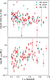 |
Fig. 2. Distributions of the observed count rate CR (top panel) and the BCG stellar mass M⋆, BCG (left panel) as functions of the cluster redshift for the eRASS1 clusters studied in this work. The clusters are colour-coded as in Fig. 1. We note that a clear dependence of the BCG stellar mass on the cluster redshift is revealed in the bottom panel, which arises from the X-ray selection primarily favoring massive clusters at high redshift. |
2.2. The HSC datasets
We used the data from the HSC survey to (1) measure the weak-lensing shear profiles and hence the weak-lensing mass, and to (2) extract the stellar mass of the BCGs. In what follows, a brief description about the datasets is provided.
In terms of the weak-lensing measurements, we used the latest HSC Three-Year (Y3) shape catalogues (Li et al. 2022) that were constructed using the i-band imaging acquired during 2014 and 2019 with a mean seeing of 0.59 arcsec. The catalogue has a limiting i-band magnitude cut of i < 24.5 mag, resulting in an average density at a level of ≈20 galaxies/arcmin2. The shape measurement was rigorously calibrated against image simulations (see e.g. Mandelbaum et al. 2018a), delivering the multiplicative bias mγ at a level of |mγ|< 9 × 10⁻³ independently of redshift up to z ≈ 3. Various null tests were examined to be consistent with zero or within the requirements for cosmic-shear analyses, ensuring sufficiently accurate weak-lensing measurements for cluster studies. The HSC-Y3 shape catalogue covers a footprint area of ≈500 deg2 and is divided into six fields, namely GAMA09H, GAMA15H, XMM, VVDS, HECTOMAP, and WIDE12H. The clusters selected in eRASS1 are only located in the fields of GAMA09H, GAMA15H, and WIDE12H, of which the datasets are used in this work.
The photometric redshift (photo-z) of the weak-lensing source sample is needed to interpret the weak-lensing measurements. Specifically, we used the photo-z estimated by the machine-learning-based code DEmP (Direct Empirical Photometric method; Hsieh & Yee 2014), whose performances were fully quantified in Nishizawa et al. (2020). In short, the bias, scatter, and the outlier fraction of the photo-z estimates for the source galaxies are estimated to be at levels of |Δz|≈0.003(1+z), σΔz ≈ 0.019(1+z), and ≈5.4%, respectively, where Δz is defined as the difference between the photometric and spectroscopic redshifts. The full distribution P(z) of the photo-z estimates was used to model the weak-lensing signals.
In Kluge et al. (2024), the BCGs of eRASS1 clusters were identified as the brightest passive member galaxies within a characteristic radius. In addition, the authors estimated that approximately 85% of eRASS1 clusters’ BCGs coincide with the optical centers. To ensure a homogeneous identification of BCGs, we visually select each cluster’s brightest galaxy as the BCG using the HSC image. Specifically, we selected the BCG of each eRASS1 cluster as the brightest galaxy whose color is similar to that of the galaxy overdensity near the X-ray centre. As a result, we find that 25 (out of 101) eRASS1 clusters in our sample have their BCGs that differ from those automatically selected in Kluge et al. (2024). As a validation, we compared the photo-z estimates (photoz_best) of the BCGs from the HSC survey with the cluster redshifts (Z_LAMBDA) and calculated the BCG photo-z bias defined as ΔzBCG ≡ (photoz_best−Z_LAMBDA)/(1+Z_LAMBDA). We find that the bias ΔzBCG has a median value of 0.0028 and a standard deviation of 0.0151, indicating that the BCG identification is robust in this work.
To estimate the stellar mass M⋆, BCG of BCGs, we used the forced cmodel photometry at the grizY broadband queried from the HSC Public Data Release 3 (PDR3). No attempts to include the intracluster light (ICL) in M⋆, BCG were made. We excluded the BCGs with pixels (in one of the grizY images) that are contaminated, saturated, or masked due to bright stars, or that have failures in the cmodel photometric fitting. This leads to a sample of BCGs with clean cmodel photometry. Aiming for the high signal-to-noise ratio and uniform HSC photometry, we only included the BCGs with at least two exposures in all grizY bands. Appendix A contains the flags used in querying the photometry of the BCGs. Appendix B shows the cutout images of these BCGs studied in this work. The identified sky locations of the BCGs are tabulated in Table B.1.
It is important to note that the cmodel algorithm adopts a composite model, where the bulge and disk components are described by de Vaucouleurs (1948) and exponential profiles, respectively. Consequently, the cmodel photometry does not fully capture the stellar distribution of the extended, diffuse ICL at large radii around BCGs. As a result, the cmodel photometry is expected to underestimate the “total” flux of a BCG+ICL system (see also Akino et al. 2022). In fact, the exact definition of the “total” stellar mass of BCGs becomes nuanced, as they are embedded within the surrounding ICL. A common approach to obtain the “total” stellar mass of a BCG+ICL system is to measure the flux within a large aperture, followed by a conversion from the observed light to the mass with an assumed mass-to-light ratio. In Huang et al. (2018a), they estimated the stellar mass profiles of BCGs using a series of well defined apertures and found that the stellar masses estimated from the cmodel photometry were systematically lower than those enclosed within 100 kpc, precisely because the cmodel photometry does not account for the extended ICL component at large radii. By stacking the light profiles of ≈3000 clusters in Chen et al. (2022), the authors found that the stellar mass of a BCG alone is well approximated by the stellar mass of the bulge/disk component enclosed within ≈50 kpc, beyond which the BCG component slowly transitions to the ICL-dominated regime at ≳100 kpc. In this study, where the cmodel photometry is used, we effectively estimate only the stellar mass of the bulge/disk components of a BCG+ICL system (within ≲50 kpc).
We note that the photometric catalogue of the BCGs is constructed independently of the HSC-Y3 shape catalogue, such that the availability of the optical photometry for the BCGs is not subject to the selection of the weak-lensing sources. Consequently, some clusters have available HSC grizY photometry to estimate the BCG stellar mass but no data to obtain the weak-lensing mass, and vice versa. The final sample of 124 eRASS1 clusters includes 23 and 28 systems with only weak-lensing data and BCG photometry, respectively; the remaining 73 clusters have both datasets.
The distributions of the X-ray count rate CR, the BCG stellar mass M⋆, BCG (which we derive in Sect. 3.2), and the cluster redshift zcl are shown in Fig. 2 with colors indicating the availability of the HSC datasets.
3. Measurements
For individual clusters with the available datasets, we extracted two kinds of measurements, the weak-lensing shear profile (Sect. 3.1) and the BCG stellar mass (Sect. 3.2).
3.1. Weak-lensing measurements
To extract the weak-lensing measurements, we followed the identical procedure as detailed in Chiu et al. (2022), in which they used the same HSC-Y3 datasets to derive the tangential reduced shear profiles g+(θ) as a function of the angular radius θ to calibrate the halo mass of clusters selected in the eROSITA Final Equatorial-Depth Survey (eFEDS; Liu et al. 2022). Later, the same weak-lensing analysis was used to derive cosmological constraints using the eFEDS cluster abundance (Chiu et al. 2023). Here, the weak-lensing data products produced in this work have been closely examined against other Stage III surveys (Kleinebreil et al. 2025) and used in the eRASS1 cosmological analyses (Ghirardini et al. 2024). In what follows, we provide a summary of the weak-lensing measurements.
On a basis of individual clusters, the weak-lensing measurements are composed of the tangential reduced shear profile g+(θ) (with the measurement uncertainty) and the corresponding redshift distribution of the source galaxies. A galaxy was selected as a weak-lensing source of a cluster at redshift zcl based on its full redshift distribution P(z), requiring it to be securely located at the background with ∫zcl + 0.2P(z)dz > 0.98. With this “P-cut” selection (Oguri 2014; Medezinski et al. 2018), the resulting source sample is extremely clean without cluster member contamination out to redshift z ≈ 1.2 (see Fig. 3 in Chiu et al. 2022). Following Eq. (8) in Chiu et al. (2022), the shear profile g+(θ) was extracted around the eROSITA-defined X-ray centre with ten logarithmic radial bins between 0.2 h−1 Mpc and 3.5 h−1 Mpc calculated in a fixed flat ΛCDM cosmology with Ωm = 0.3 and h = 0.7. The three innermost bins were discarded in the weak-lensing mass modelling to avoid systematics, resulting in total seven logarithmic bins at a radial range of 0.5 h−1 Mpc ≲ R < 3.5 h−1 Mpc. We note that we converted the unit of the radial binning to the angular space, i.e. in arcmin, and self-consistently fitted the model of the cluster mass profile at a correct physical scale inferred from the redshift-distance relation while the cosmological parameters are varying in the forward modelling. The uncertainty of the tangential shear profile is expressed by the weak-lensing covariance matrix (see Eq. (14) in Chiu et al. 2022); however, we only include the shape noise, as opposed to that in Chiu et al. (2022) containing the scatter due to uncorrelated large-scale structures (Hoekstra 2003). The scatter raised from uncorrelated large-scale structures is accounted for in calibrating the weak-lensing mass bias (see Sect. 4.3 and Grandis et al. 2024). The stacked and lensing-weight-weighted P(z) of the source galaxies for each cluster is used to infer the lensing efficiency (see Eq. (34) in Chiu et al. 2022).
We describe the modelling of these shear profiles to calibrate the cluster halo mass in Sect. 4.3.
3.2. Measurements of BCG stellar masses
Similarly to the procedure in Chiu et al. (2018, see also Erfanianfar et al. 2019), we estimated the BCG stellar mass M⋆, BCG using the SED (spectral energy distribution) fitting technique implemented in the χ2 template-fitting code, Le Phare (Arnouts et al. 1999; Ilbert et al. 2006)2. We describe the analysis steps below.
We used the five broadband photometry grizY from the PDR3 database of the HSC survey. For each BCG, the template fitting is fixed to the cluster redshift zcl. The SED fitting has two passes. The first is to account for the zero-point offsets in the photometry. Specifically, we built the galaxy templates from the COSMOS field (Ilbert et al. 2009) with the Prevot et al. (1984) and Calzetti et al. (2000) dust-extinction laws3 with E(B−V) in a range between 0 and 0.5. Once the best-fit template was determined for each BCG, a systematic zero-point offset of each band was computed to minimize the differences between the models and observed magnitudes among all the BCGs. This process was iterated until a convergence is reached. The second pass of the SED fitting is to obtain the BCG stellar mass by fitting the galaxy templates predicted by the Stellar Population Synthesis (SPS). We built the SPS templates using the Bruzual & Charlot (2003) model with the Chabrier (2003) initial mass function (IMF). Three metallicities (Z = 0.004, 0.008, 0.02) are used and configured with the exponentially decaying star-formation rate characterized by an e-folding timescale τ. We used six values of τ up to 5 Gyr (i.e.  ) because BCGs are expected to be dominated by old stellar populations without recent star-forming activities. This is supported by our data, as extending the timescale τ to 30 Gyr to include star-forming galaxy templates does not change the final results (see Sect. 5). Moreover, the galaxy templates are configured with the Calzetti et al. (2000) dust-extinction law of E(B−V) = 0, 0.1, 0.2, 0.3. The ages of these galaxy templates can have a maximum value of 14 Gyr. When fitting the Bruzual & Charlot (2003) templates, we apply the zero-point offsets obtained from the first pass to the individual bands and add the same amounts of systematic uncertainties to the measurement uncertainties in quadrature. We note that this effectively weakens the constraining power of the bands with a larger offset. Last, we increased the flux uncertainties (after adding the systematic uncertainties) by a factor of 6.5, which is suggested by our data, such that the median of the resulting reduced χred2 of the BCGs is unity. This does not change the best-fit stellar mass but only increases the measurement uncertainty of the final mass estimate. We note that the statistical uncertainties of the photometric measurements of the BCGs in the grizY bands are at a level of 10−3 mag, and that the SED templates predicted by SPS are not perfect. As a result, even small discrepancies between the model and observation can lead to significantly large χred2. By increasing the flux uncertainties while requiring the median χred2 of the sample to be unity, we effectively account for the uncertainty in the derived stellar mass arising from the limitations of the SED templates. The measurement uncertainty of M⋆, BCG is obtained by bootstrapping the Bruzual & Charlot (2003) template fitting by 1000 times, assuming that the flux uncertainties are Gaussian.
We estimated the systematic uncertainty in our stellar mass measurements as follows. We constructed a catalogue of galaxies observed in the COSMOS field from the HSC data base, estimate their stellar masses at known redshifts using the same method mentioned above, and compare the resulting stellar masses M⋆, HSC to those in the latest COSMOS2020 catalogue (M⋆, COSMOS) estimated using 30-band photometry (Weaver et al. 2022). In the stellar mass and redshift range occupied by the BCGs of the eRASS1 clusters ( and z ≲ 1), we find a systematic offset in the stellar mass at a level of ≈0.1 dex, i.e. ⟨log(M⋆, HSC/M⊙)−log(M⋆, COSMOS/M⊙)⟩ ≈ 0.1 dex. Moreover, this systematic offset does not depend on the redshift. Therefore, we expect that (1) there exists a systematic uncertainty at a level of ≈0.1 dex in our M⋆, BCG estimates with respect to those measured with the full configuration of SED templates on high-quality data such as in the COSMOS field, and that (2) the systematic uncertainty only affects the normalization but not the mass or redshift trends of the scaling relation.
The resulting BCG stellar mass estimates M⋆, BCG are plotted as a function of the cluster redshift in Fig. 2. We present the results of the SED fitting in Appendix B. The measurements of the BCG setllar mass M⋆, BCG of individual eRASS1 clusters are contained in Table B.1.
4. Modelling
Our goal is to constrain the scaling relations of the observables, including the X-ray count rate CR and the BCG stellar mass M⋆, BCG. We first provide an overall framework of the modelling in Sect. 4.1, and refer to Chiu et al. (2022, see also Bocquet et al. 2019 and Chiu et al. 2023) for more details. Next, we describe the modelling of the scaling relations in Sect. 4.2, followed by the description of the weak-lensing modelling in Sect. 4.3. Finally, we give the statistical inference to obtain the parameter posteriors in Sect. 4.4.
4.1. Modelling framework
The cluster sample is constructed based on the X-ray selection (Lext > 6) with the aid of the optical confirmation to remove the contamination with unphysically low richness (λ ≤ 3), together with the selection of the cluster redshift at 0.1 < z < 0.8 (see Sect. 2.1 and Sect. 2.1 in Ghirardini et al. 2024). The extent likelihood Lext is mainly subject to the parameters tuned to optimize in the cluster-finding algorithm and lacks a straightforward association with the physical properties of clusters. Therefore, it is not an ideal mass proxy. Instead, we use the observed X-ray count rate CR as the mass proxy. Meanwhile, the intrinsic X-ray count rate  acts as an X-ray “selection” observable. The observed CR and intrinsic
  are related through the measurement uncertainty, and both can serve as selection observables.
In short, there are three selection observables  , where the uncertainty of the cluster redshift z is negligible, and the richness selection mainly removes obvious contamination with an insignificant impact on the resulting sample (Ghirardini et al. 2024). That is, the cluster selection is primarily determined in X-rays.
The follow-up observations of individual clusters are then conducted to obtain the follow-up observables, which are the weak-lensing shear profile g+ and the BCG stellar mass M⋆, BCG in this study. It is extremely important to note that the follow-up observables are uniformly obtained for every cluster and that the lack of these follow-up observables for some clusters does not rely on any preferences for X-ray properties. In other words, no additional selections are made on the weak-lensing shear profile g+ and the BCG stellar mass M⋆, BCG.
We denote the selection and follow-up observables by the symbols of 𝒮 and 𝒪, where 𝒮 ≡ {CR,λ,z} and 𝒪 ≡ {g+,M⋆, BCG}, respectively. For the scaling relations parametrized by a parameter vector p, we maximize the probability of observing the follow-up observable 𝒪 for a cluster selected with the selection observable 𝒮 as
 (1)
(1)
where the label N represents the number of clusters with the observables of 𝒮 and/or 𝒪 evaluated at the parameter vector p.
Equation (1) is referred to as the “mass calibration likelihood” widely used in the population modelling of galaxy clusters (e.g. Chiu et al. 2022, 2023; Ghirardini et al. 2024). Consider the selection function as a function of only the observed quantity 𝒮 rather than the intrinsic one  . Because the selection of the clusters purely depends on 𝒮 instead of 𝒪, the selection-function factors of both the numerator and denominator in Eq. (1) are cancelled4 and have no effect (see Eq. (3) in Chiu et al. 2023). That is, the selection function of the cluster sample is not important for the mass calibration likelihood, i.e. Eq. (1), as long as no additional selection is made on the follow-up observable 𝒪, as in this study.
In this study and other eRASS1 work, however, the selection function  is calibrated at the sky location ℋ and redshift z of each cluster in terms of the intrinsic observable, namely the intrinsic count rate
  (Clerc et al. 2024). Therefore, the selection function is implicitly used in calculating both the numerator and denominator of Eq. (1) and cannot be canceled. We note that the selection function
  does not depend on the parameter vector p, which is distinct from the self-calibrated selection function used in Chiu et al. (2023).
Because (1) we ignore the uncertainty of the cluster redshift and (2) the richness selection of λ > 3 has no impact on the resulting X-ray selected sample (Ghirardini et al. 2024), Eq. (1) can be approximated with 𝒮 = {CR,z} as (e.g. Eq. (56) in Chiu et al. 2022)
 (2)
(2)
where n(M|z,p) is the halo mass function evaluated at the cluster redshift z and the parameter vector p.
In Eq. (2), the factor P(CR|M,z,p) describes the probability of observing the X-ray count rate CR given the halo mass M at the redshift z evaluated with the parameter vector p. It includes two components making the observed count rate CR scatter around the mean value predicted at the fixed cluster mass and redshift. The first is the intrinsic scatter in the count rate, and the second is the measurement uncertainty due to the observational noise. Additionally, we include the selection function in terms of the intrinsic count rate  at the redshift z and the sky location ℋ, i.e.
  . Therefore, we further deduce the probability P(CR|M,z,p) as
 (3)
(3)
where  describes the intrinsic count rate
  scattering around the mean value predicted at the fixed cluster mass M and redshift z, and the
  accounts for the scatter due to the measurement uncertainty. The count rate-to-mass-and-redshift (CR–M–z) relation is modelled in Sect. 4.2. We assume a log-normal and constant intrinsic scatter σX in the X-ray count rate, as no significant variation of σX as a function of M and z is suggested (Chiu et al. 2022, 2023; Ghirardini et al. 2024).
Similarly, the factor P(M⋆, BCG,g+,CR|M,z,p) in the numerator of Eq. (2) describes the probability of observing the observables {M⋆, BCG,g+,CR} at the fixed cluster mass M and redshift z given the parameter vector p, which reads
![Mathematical equation: $$ \begin{aligned}&P\left(M_{\star ,\mathrm{BCG} }, {g_{+}}, C_{\mathrm{R} } | {M}, {z}, \mathbf p \right)\nonumber \\&= \int \int \int \Big [ P\left(M_{\star ,\mathrm{BCG} } | \hat{M}_{\star ,\mathrm{BCG} } \right) P\left({g_{+}} | M_{\mathrm{WL} }, {z}, \mathbf p \right) P\left(C_{\mathrm{R} } | \hat{C}_{\mathrm{R} } \right) \times \Big . \nonumber \\&\Big . \mathcal{I} _{{z}}\left(\hat{C}_{\mathrm{R} }\right) P\left(\hat{M}_{\star ,\mathrm{BCG} }, M_{\mathrm{WL} }, \hat{C}_{\mathrm{R} } | {M}, {z}, \mathbf p \right) \Big ] \mathrm{d} \hat{M}_{\star ,\mathrm{BCG} }\ \mathrm{d} M_{\mathrm{WL} }\ \mathrm{d} \hat{C}_{\mathrm{R} }\ \, . \end{aligned} $$](/articles/aa/full_html/2025/12/aa54942-25/aa54942-25-eq22.gif) (4)
(4)
In Eq. (4), the probability  describes the joint intrinsic distribution of the observables
  at the fixed cluster mass M and redshift z, the factor
  takes the measurement uncertainty of the BCG stellar mass into account, and P(g+|MWL,z,p) accounts for the measurement uncertainty of the shear profile, expressed by the weak-lensing covariance matrix (Sect. 3.1). The selection function
  is also included to calculate Eq. (4).
The correlations between the intrinsic scatters of the observable pairs of the X-ray count rate and the BCG stellar mass (ρX, BCG), the X-ray count rate and the weak-lensing mass (ρX, WL), and the BCG stellar mass and the weak-lensing mass (ρBCG, WL) are included in calculating the joint intrinsic distribution,  .
.
We provide the following remarks for Eq. (4). First, P(g+|MWL,z,p) models the observed shear profile g+(θ) by a mass profile given the weak-lensing mass MWL and the redshift z. This requires a redshift-distance relation, which has dependence on cosmological parameters, to compare the mass profile in the physical scale with the observed shear profile in the angular scale. Moreover, the mass model includes nuisance parameters to account for the miscentring effect, for example. We therefore keep the parameter vector p in P(g+|MWL,z,p) to account for the measurement uncertainty of the shear profile. Second, the weak-lensing mass MWL, the mass estimate that best describes the observed shear profile, is not equal to the cluster halo mass M that is used to parametrize the halo mass function. This is because the halo model is not a perfect description of observed galaxy clusters; for example, the clusters have substructures or triaxiality that are not included in the model (see Sect. 4.2 in Chiu et al. 2022). This leads to a biased weak-lensing mass MWL with respect to the cluster halo mass M. Such weak-lensing mass bias is accounted for by the weak-lensing mass-to-halo mass relation given in Sect. 4.3. Third, the measurement uncertainty of the BCG stellar mass is modelled as a Gaussian noise in terms of the ten-based logarithmic BCG stellar mass, i.e. log(M⋆, BCG).
For the clusters with only the observed shear profile g+, the modelling of the BCG stellar mass is omitted in Eq. (4), finally leading to
 (5)
(5)
For those clusters with only the BCG stellar mass estimates, we have
 (6)
(6)
4.2. Modelling of the scaling relations
In this work, we use three scaling relations to model the cluster observables as functions of the halo mass and redshift. They are the count rate-to-mass-and-redshift (CR–M–z) relation, the BCG stellar-mass-to-mass-and-redshift (M⋆, BCG–M–z) relation, and the weak-lensing mass bias-to-mass-and-redshift (bWL–M–z or MWL–M–z) relation. These scaling relations are constrained at the pivotal mass Mpiv and redshift zpiv, where we use  and zpiv = 0.35 throughout this work. The correlated intrinsic scatters among these observables are also included in the modelling (see Sect. 4.1).
4.2.1. The count rate-to-mass-and-redshift relation
For the CR–M–z relation, we use the same functional form as in the eRASS1 cosmological analysis (Ghirardini et al. 2024), namely
 (7)
(7)
where AX is the normalization with a unit of counts/sec at the pivotal mass Mpiv and redshift zpiv, BX is the power-law index of the mass trend with a redshift-dependent slope parametrized by δX, γX describes the power-law scaling of the redshift trend, DL denotes the luminosity distance, and E(z) accounts for the self-similar redshift evolution of the X-ray luminosity (Kaiser & Silk 1986; Böhringer et al. 2012). We adopt a log-normal and constant intrinsic scatter,  , around the mean value predicted by Eq. (7) at a fixed mass M and redshift z.
4.2.2. The BCG stellar-mass-to-mass-and-redshift relation
For the M⋆, BCG–M–z relation, or the stellar-mass-to-halo-mass relation, we use the power-law functional form as
 (8)
(8)
where ABCG is the normalization in a unit of dex, BBCG is the power-law index of the mass trend with a redshift-dependent slope parametrized by δBCG, and γBCG describes the power-law slope of the redshift scaling. We assume a log-normal and constant intrinsic scatter σBCG around the mean value predicted by Eq. (8). Although ABCG is in units of dex, we express the intrinsic scatter in terms of the natural log, i.e.  , in the interest of consistency with the other scaling relations. We note that the parametrization of the redshift-dependent mass slope in Eq. (8), i.e.
  , is a result of following that used in Moster et al. (2013, see their Eq. 14). We have tried a different functional form, ln(1+z)/(1+zpiv), for the redshift-dependent mass slope and find no significant impact on the final results and our conclusions.
4.2.3. The weak-lensing mass bias-to-mass-and-redshift
For the weak-lensing mass bias  , we follow the identical functional form developed in Grandis et al. (2024) and also applied to the cosmological analysis in Ghirardini et al. (2024), as
 (9)
(9)
where BWL describes the mass trend of the weak-lensing mass bias, and lnbz(z|δWL,γWL) is the redshift-dependent normalization of the mass bias parametrized by two parameters, δX and γX, as
 (10)
(10)
in which the notation ℑ(x0|x,y) stands for the linear interpolation at x0 among the function that has the values y at x. In Grandis et al. (2024), they calibrated the weak-lensing mass bias using simulated clusters extracted at four snapshots of redshift, which we label them by zsim in Eq. (10), and derived the mass bias μ0 with the two principle components μ1 and μ2 characterizing the uncertainty. In this way, the distribution of the weak-lensing mass bias as a function of the cluster redshift can be evaluated by directly interpolating among the redshift snapshots zsim with the parameters of δWL and γWL modelled by Gaussian distributions of 𝒩(0,12). While the mean weak-lensing mass bias at the halo mass M and redshift z is calculated with Eqs. (9) and (10), we model the intrinsic scatter of the weak-lensing mass around the mean value by a log-normal and constant scatter as  . This modelling is different from those in Grandis et al. (2024) and Kleinebreil et al. (2025), where the intrinsic scatter of the weak-lensing mass was modelled as a function of the halo mass and redshift. This modification is consistent with the modelling of the cluster miscentring, for which we also adopt a fixed model globally for all eRASS1 clusters (see Sect. 4.3 for details). As seen in Sect. 5.1, the results of our modelling with a statistical approach fully agree with those of Kleinebreil et al. (2025), which used a method dependent on individual clusters.
4.3. Weak-lensing modelling
In this subsection, we describe (1) the modelling of the shear profile to obtain the weak-lensing mass MWL, and (2) the calibration of the weak-lensing mass bias bWL. For the former, we closely follow the fitting procedure detailed in Chiu et al. (2022) with minor modifications to be consistent with that adopted in Ghirardini et al. (2024). Meanwhile, the latter task has been quantified in Grandis et al. (2024, see also Grandis et al. 2021) and applied to the weak-lensing mass calibration of eRASS1 clusters (e.g. Kleinebreil et al. 2025) as well as the cosmological analyses (Ghirardini et al. 2024). We briefly summarize them, as follows.
Given a cluster at redshift zcl and a background population with a stacked (and lensing-weight-weighted) redshift distribution P(z), the model  of the tangential reduced shear profile as a function of the projected (physical) radius R is calculated with a parameter vector p5 as
 (11)
(11)
in which β is the lensing efficiency depending on the angular diameter distance6,
 (12)
(12)
and  and κmod are the models of the tangential shear and convergence, respectively, which read
 (13)
(13)
 (14)
(14)
where  is the model of the surface mass density at the projected radius R, Σcrit is the critical surface mass density,
 (15)
(15)
and  is the excess surface mass density,
![Mathematical equation: $$ \begin{aligned} {\Delta {\Sigma }_{\mathrm{m}}^{\mathrm{mod}}}\left({R} | \mathbf p \right) \equiv \left[ \frac{2}{{R}^2}\int _0^{{R}}{\Sigma }_{\mathrm{m}}^{\mathrm{mod}}\left(x | \mathbf p \right)x\mathrm{d} x \right] \ - {\Sigma }_{\mathrm{m}}^{\mathrm{mod}}\left({R} | \mathbf p \right) \, . \end{aligned} $$](/articles/aa/full_html/2025/12/aa54942-25/aa54942-25-eq49.gif) (16)
(16)
In Eq. (11), the quantities of ⟨β(p)⟩ and ⟨β2(p)⟩ are obtained with the weights of the background redshift distribution P(z),
 (17)
(17)
 (18)
(18)
The projected and physical radius R is determined as R = DA(zcl|p) × θ, where the θ is the clustercentric radius in a unit of radian. The comparison between the observed shear profile and the model is in the space of the angular radius θ, and therefore the redshift-distance relation must be used to correctly calculate the physical radius at a fixed θ and a given parameter vector p.
The model of the projected surface mass density  is composed of two components, the perfectly centered profile
  and that with the miscentring
  . They are weighted by the fraction fmis of the miscentered clusters, in a statistical approach, as
 (19)
(19)
where  is modelled by a spherical Navarro–Frenk–White (hereafter NFW; Navarro et al. 1997) profile, and
  is modelled by a miscentered NFW model (see e.g. Johnston et al. 2007) with a characteristic and dimensionless miscentring scale σmis (see Eq. (20) in Chiu et al. 2022), which is a varied parameter in p.
There are minor modifications from the previous study, Chiu et al. (2022). First, a different halo concentration-to-mass (c–M) relation is used when calculating the NFW profile. Here, we use the mean value predicted by the c–M relation from Ragagnin et al. (2021) at a given weak-lensing mass MWL and the cluster redshift as the halo concentration, while they used the c–M relation from Diemer (2018). Second, we only include shape noises in the weak-lensing covariance matrix, as the measurement uncertainty of the observed shear profile. The scatter (denoted as ℂLSS) in the shear profile due to uncorrelated large-scale structures along the line of sight is accounted for when calibrating the weak-lensing mass bias. To be exact, the scatter ℂLSS calculated from the formula in Hoekstra (2003) is included in fitting the weak-lensing shear profile of simulated clusters when calibrating bWL (see Sect. 2.1.6 in Grandis et al. 2021). Consequently, the resulting scatter of bWL naturally includes the effect of uncorrelated line-of-sight structures. In Chiu et al. (2022), the scatter ℂLSS was calculated and initially included in the weak-lensing covariance matrix as a component of the measurement uncertainty. These two merely differ in the philosophy of the methodology, not the final results. Third, we update the miscentring model to that determined for the eRASS1 sample. Specifically, the miscentring of the eRASS1 clusters was calibrated using the synthetic X-ray eROSITA images of clusters in the eROSITA digital-twin simulations (Grandis et al. 2024, see also simulations produced in Comparat et al. 2019, 2020; Seppi et al. 2022), including both intrinsic and observational effects. As a result, the miscentring of clusters was expressed by the probability fmis of being miscentered and a characteristic miscentring scale σmis that depends on the extent EXT and the detection likelihood Ldet, two quantities returned by the eRASS detection pipeline.
The purpose of the first two aforementioned changes is to use the identical c–M relation and the measurement uncertainty as in Grandis et al. (2024), where the dedicated and updated calibration of the weak-lensing mass bias was carried out. Meanwhile, for the third modification we implement the miscentring model in a statistical approach to have a much speedier calculation. That is, we first calculate the distribution of the characteristic miscentring scale σmis of our eRASS1 sample based on the miscentring calibration (see Sect. 4.2 in Grandis et al. 2024), model it as a log-normal distribution, and apply the result as an informative Gaussian prior on lnσmis in Eq. (19) for all the clusters consistently. Similarly, we also do so for the parameter of the miscentring fraction fmis for our eRASS1 sample. The resulting Gaussian priors on fmis and lnσmis are 𝒩(0.32,0.0432) and 𝒩(−0.85,0.182), respectively. This approach is equivalent to statistically correcting for the miscentring effect at a population level. Because we also model the scatter of the weak-lensing mass bias in the same way (see the last paragraph), we do not expect a significant impact on the final results from this modification. Indeed, our result is in excellent agreement with Grandis et al. (2024) and Kleinebreil et al. (2025), as seen in Sect. 5.1.
As fully described in Grandis et al. (2024, see also Grandis et al. 2021), the weak-lensing mass bias, bWL ≡ MWL/M, is calibrated by repeating the same modelling on the synthetic shear profiles of clusters extracted from the cosmological hydrodynamical TNG300 simulations (Pillepich et al. 2018), of which the underlying halo mass M used to parametrize the halo mass function is known. The bias and intrinsic scatter of the weak-lensing mass are derived, specifically tailored to include the observational effects of (1) the misfitting due to the halo triaxiality or shape, (2) the miscentring of the eROSITA X-ray centre, (3) the cluster member contamination7, (4) the photo-z bias of the background sources, (5) the calibration uncertainty of the galaxy shape measurement. Importantly, the systematic uncertainties of the resulting weak-lensing mass bias and scatter include baryonic effects. This is achieved by quantifying the systematic difference in the results of the bWL calibrations between the same suite of the dark-matter-only and hydrodynamical simulations. In the end, the constraints on the parameters of Eqs. (9) and (10) are obtained and applied as informative priors in the final modelling. The resulting constraints are tabulated in Table A.3. of Kleinebreil et al. (2025).
In terms of the intrinsic scatter σWL of the weak-lensing mass bias, Grandis et al. (2024) parametrized σWL as a function of the cluster mass M and redshift z. In this work, we adopt a constant and average weak-lensing mass scatter σWL without modelling its mass and redshift dependence. This is a reasonable approach, given that we do not observe significant mass-dependent scatter and that the scatter σWL is statistically constant out to redshift z ≈ 0.8 (see Table A.3 in Kleinebreil et al. 2025). In practice, we calculate the distribution of the weak-lensing bias scatter of our eRASS1 sample based on the resulting model reported in Kleinebreil et al. (2025), and model it as a Gaussian distribution that we apply as an informative prior on σWL in the final modelling. For our sample, we find that σWL can be well described by 𝒩(0.23,0.032).
4.4. Statistical inference
We adopt the Bayesian framework to explore the posterior P(p|𝒟) of the parameter vector p given the observed data vectors 𝒟,
 (20)
(20)
where ℒ(𝒟|p) is the likelihood of observing 𝒟 at a given p, and 𝒫(p) is the prior on p. In this work, the data vector 𝒟 consists of both the selection and follow-up observables 𝒮 and 𝒪 of individual clusters, i.e. 𝒟 = {𝒮i,𝒪i|i∈eRASS1 clusters}. We use the importance nested sampler Multinest (Feroz et al. 2009) implemented in the CosmoSIS framework (Zuntz et al. 2015) to explore the likelihood.
With the technique of the population modelling, i.e. jointly fitting individual clusters at the same time, we calculate the log-likelihood with Eqs. (2), (5), and (6) as
 (21)
(21)
where zcl is the cluster redshift (and fixed to its photometric redshift), i runs over the clusters with both the measurements of the weak-lensing shear profile g+ and the BCG stellar mass M⋆, BCG, and j and k run over those with only g+ and M⋆, BCG, respectively. The parameter vector p includes the parameters8 of
-
{AX,BX,δX,γX,σX} of the CR–M–z relation in Eq. (7),
-
{ABCG,BBCG,δBCG,γBCG,σBCG} of the M⋆, BCG–M–z relation in Eq. (8),
-
{BWL,δWL,γWL,σWL} of the MWL–M–z relation in Eq. (9),
-
{fmis,lnσmis} of the weak-lensing miscentring modelling in Eq. (19), and
-
{#x03A9;m,h,σ8,Ωb,ns} of the cosmological parameters in a flat ΛCDM model.
We adopt the following priors. For the cosmological parameters, we apply flat priors, namely 𝒰(0.10,0.99), 𝒰(0.03,0.07), 𝒰(0.50,0.90), 𝒰(0.94,1.0), and 𝒰(0.45,1.15) to Ωm, Ωb, h, ns, and σ8, respectively. Additionally, Gaussian informative priors of 𝒩(0.3,0.022), 𝒩(0.8,0.022), and 𝒩(0.7,0.052) are applied to Ωm, σ8, and h, respectively. With these informative priors, the cosmological parameters of the flat ΛCDM model are effectively anchored to the widely accepted concordance values with the uncertainties of (Ωm,σ8,h) at levels of those obtained from the state-of-the-art constraints.
For the parameters of the weak-lensing mass bias, we apply a Gaussian prior 𝒩(0.047,0.0212) on the mass-dependent power-law index BWL calibrated in Grandis et al. (2024) (and tabulated in Table A.3 of Kleinebreil et al. 2025). A unit Gaussian prior 𝒩(0,12) is applied on both γWL and δWL, by construction. A Gaussian prior 𝒩(0.23,0.032), informed by the eRASS1 sample we study in this work (see Sect. 4.3), is applied on the intrinsic scatter σWL of the weak-lensing mass bias.
We apply Gaussian priors of 𝒩(0.32,0.0432) and 𝒩(−0.85,0.182) to the parameters of the weak-lensing miscentring model, fmis and lnσmis, respectively (see Sect. 4.3). We required that the determinant of the correlated intrinsic scatter matrix be positive when jointly fitting the observables CR, g+, and M⋆, BCG of a cluster.
For the other parameters, only flat priors were used. We summarize the adopted priors in Table 1. These priors are similar to those used in Chiu et al. (2022) with a major difference: We only applied the flat prior to the intrinsic scatter σX of the X-ray count rate in this work, while Chiu et al. (2022, and the cosmological analysis in Chiu et al. 2023) additionally applied a Gaussian prior 𝒩(0.3,0.082) to σX.
Priors used in the default modelling.
5. Results and discussions
In a forward-modelling framework, we constrain both the CR–M–z and M⋆, BCG–M–z relations while accounting for the weak-lensing mass bias and scatter via the bWL–M–z relation. In Sect. 5.1 we first present the weak-lensing calibrated CR–M–z relation without the modelling of M⋆, BCG–M–z relation, as an analysis of purely weak-lensing mass calibration. Finally, We present the M⋆, BCG–M–z relation and discuss its implication in Sect. 5.2.
5.1. The CR–M–z relation
Regardless of the BCG stellar mass estimates, there are 96 eRASS1 clusters with available weak-lensing shear profiles. Sampling the joint likelihood of those 96 clusters, i.e. Eq. (5), without the modelling of the M⋆, BCG–M–z relation delivers the constraints on the parameters of the CR–M–z relation in Eq. (7) as
 (22)
(22)
These numbers are listed in Table 2. The marginalized posteriors of and the two-dimensional joint posteriors among these parameters are shown as the blue contours in Fig. 3, while we present the full results of the weak-lensing-only modelling in Appendix C. The correlated intrinsic scatter between the X-ray count rate and the weak-lensing mass is constrained as  , suggesting that the correlation between the X-ray and WL properties at a fixed halo mass is consistent with zero or ill-constrained in this work.
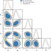 |
Fig. 3. Parameter marginalized posteriors (diagonal) and two-dimensional joint posteriors (off-diagonal) from different modelling are presented. The results of the weak-lensing mass calibration alone are shown as the blue contours, while the inclusions of the modelling of the M⋆, BCG–M–z relation are indicated by the red contours. We also indicate the results from Kleinebreil et al. (2025), based on the identical cluster sample and the weak-lensing data g+, as the green contours. |
In Fig. 3 we find excellent agreement between this work and Kleinebreil et al. (2025, the green contours). We note that Kleinebreil et al. (2025) performed the weak-lensing mass calibration of the same sample of the 96 eROSITA clusters overlapping the HSC-Y3 footprint based on the identical weak-lensing shear profiles extracted in this work. The main difference is that they modelled (1) the miscentring on a per-cluster basis depending on the X-ray detection likelihood Ldet and extent EXT and (2) the redshift-dependent intrinsic scatter of the weak-lensing mass. Meanwhile, we derive the Gaussian priors for the sample and applied them to the parameters at a population level in the modelling (see Sect. 4.3). As a result, these two results obtained from independent codes are fully consistent, again ensuring the robustness of the weak-lensing modelling.
In Fig. 4 we present the stacked shear profiles and best-fit models in four sub-samples defined by the observed count rates and redshift in the left panel. We use the median count rate (CRmed ≈ 0.487) and redshift (zmed ≈ 0.27) of the eRASS1 clusters to split the sample into four bins. The stacked shear profile for each sub-sample is calculated as the weighted average of the individual shear profiles g+, where the weights are defined as the inverse square of the radially dependent shape noise. The best-fit models, with their uncertainties fully marginalized over all parameters, are shown as the grey shaded regions. Similarly, we produce the stacked profile of all the 96 eRASS1 clusters in the right panel. As seen, we find good agreement between the stacked profiles and our best-fit models, suggesting that the weak-lensing modelling provides excellent description of the data.
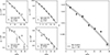 |
Fig. 4. Observed shear profiles g+ (black data points) and best-fit models with fully marginalized uncertainties (grey shaded regions). The four subplots in the left panel present the stacked profiles of the subsamples defined with respect to the median values of the observed count rate (CR = 0.487) and the redshift (z = 0.27). The stacked profile of all 96 eRASS1 clusters is presented in the right panel. The numbers of the clusters in the (sub)samples and the reduced χred2 are shown in the lower left corners. In both left and right panels, the radial values (the x-axis) of the measurements are obtained with the inverse-variance weights of the clusters in the (sub)samples. |
In Fig. 5 we present the mass and redshift trend of the CR–M–z relation re-scaled at the pivotal redshift zpiv = 0.35 and mass  in the left and right panels, respectively. The data points are eRASS1 clusters with their halo mass M randomly sampled from the mass posterior P(M|CR,g+,p) with the uncertainties fully marginalized over the posteriors of the parameters p (see Eq. (66) in Chiu et al. 2022). To show the mass trend (left panel), on the y-axis we remove the redshift dependence by dividing the observed count rate CR by the redshift-dependent factors evaluated at the best-fit parameters; similarly, we remove the mass dependence of CR to show the redshift trend in the right panel. As seen in the left panel, our results suggest a mass trend with a power-law index of
  , which is significantly steeper than the self-similar prediction at the soft X-ray band (BX = 1; the red dashed line). Meanwhile, no significant departure from the self-similar prediction of the redshift trend is revealed in the right panel (
 ), despite the large error bar. Additionally, we find no clear evidence for the cross-scaling between the halo mass and redshift (δX = 0.7 ± 1.5). The mass trend of the X-ray count rate steeper than the self-similar prediction implies that non-gravitational process (e.g. feedback from cluster cores) plays a key role in the X-ray emission. Moreover, this mass scaling this mass scaling neither depends on redshift nor deviates from the self-similar redshift evolution, implying that the non-gravitational mechanisms in massive clusters are already in place at high redshift (z ≈ 0.8 for our cluster sample). This picture is in excellent agreement with previous studies of eROSITA-selected samples (Chiu et al. 2022) and SZE-selected clusters (Bulbul et al. 2019) which probed an even higher redshift to z ≈ 1.3.
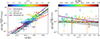 |
Fig. 5. CR–M–z relation of the eRASS1 clusters and the best-fit model in Eq. (22). Its fully marginalized uncertainties are shown as grey shaded regions. The left panel shows the mass trend normalized at the pivotal redshift zpiv = 0.35 after accounting for the redshift-dependent factors, while the right panel similarly presents the redshift scaling normalized at the pivotal mass |

In Fig. 5 the black dotted lines represent the result from Chiu et al. (2022), which were obtained based on ≈300 eROSITA-selected clusters and groups in the eFEDS survey using the same HSC-Y3 WL data. We find satisfactory agreement between Chiu et al. (2022) and this work with the following remarks. First, Chiu et al. (2022) used a slightly different functional form to model the CR–M–z relation. Specifically, they included a simulation-calibrated correction factor for the observed count rate to probe the underlying true count rate relation in eFEDS (see Sect. 4.1 in Chiu et al. 2022). Consequently, their resulting mass and redshift trends are scaled as ∝MBX − 0.16 and ∝z0.42(1+z)γX, respectively, where they contained  and
and  . In this work, we directly relate the observed count rate CR to the halo mass without the correction factor. In Fig. 5 we plot the overall mass and redshift trends of Chiu et al. (2022) as
  and
and  , respectively. Second, as the major difference between Chiu et al. (2022) and the updated analysis of eRASS clusters in this study (also Grandis et al. 2024; Kleinebreil et al. 2025), the former applied a Gaussian prior 𝒩(0.3,0.082) to the intrinsic scatter σX, as opposed to this work in which only an uninformative prior 𝒰(0.05,2.0) is adopted. Removing the Gaussian prior reveals a significantly large intrinsic scatter σX ≳ 0.55 as preferred by the count rate observed by eROSITA (see also Grandis et al. 2024; Kleinebreil et al. 2025). Meanwhile, there exists a strong degeneracy between the normalization AX and σX (as seen in Fig. 3), leading to a lower AX with increasing σX in this work. As seen in Fig. 5, we obtain a normalization AX mildly lower than Chiu et al. (2022,
  ) at a level of ≈1.6σ.
It is worth mentioning that the large intrinsic scatter σX results in significant Eddington (1913) bias, as evident from the offset between the sampled masses P(M|CR,g+,p) and the best-fit CR–M–z relation in Fig. 5. This is explained by the posterior P(M|CR,g+,p) evaluated as P(M|CR,g+,p) ∝ P(CR,g+|M,p)P(M|p), where P(M|p) is the normalized halo mass function. At a fixed halo mass, the large scatter σX of the observed count rate leads to a wide distribution P(CR,g+|M,p) so that the up-scatter contribution from the low-mass end of the halo mass function P(M|p) becomes significant. Consequently, the sampled masses (data points) are expected to be lower than those following the best-fit CR–M–z relation (grey region) at a given fixed count rate in the left panel. The Eddington bias is accounted for in this work and other eROSITA analyses, thus the resulting scaling relations are unbiased. An even larger intrinsic scatter of σX ≈ 1 was found in Ghirardini et al. (2024), where the authors combined the weak-lensing mass calibration and the abundance of eRASS1 clusters to constrain cosmological parameters. It is surprising that the intrinsic scatter of the eROSITA observed count rate, obtained from either weak lensing alone or a combination with the cluster abundance, is significantly larger than that (≈0.3) of X-ray luminosity in previous studies (Pratt et al. 2009; Vikhlinin et al. 2009b; Lovisari et al. 2015; Mantz et al. 2016; Bulbul et al. 2019; Chiu et al. 2022; Bahar et al. 2022; Akino et al. 2022). This implies that significantly large scatter is introduced in measuring the X-ray count rate in the eROSITA data pipeline, increasing the intrinsic scatter at a fixed halo mass from a scale of 30% in the X-ray luminosity to a factor of exp(1) ≈ 2.7 in the count rate. A future study investigating this topic is warranted.
We show the comparisons with the weak-lensing-calibrated results of eRASS1 clusters using data from the DES (Grandis et al. 2024, the green lines) and KiDS (Kleinebreil et al. 2025, the purple lines) surveys in Fig. 5. We observe excellent agreement with the DES result as they constrained AX = 0.088 ± 0.02, BX = 1.62 ± 0.14, δX = −0.85 ± 0.93, γX = −0.32 ± 0.69, and σX = 0.61 ± 0.19. Meanwhile, mild discrepancy at ≲1.5σ is seen between this work the KiDS result with their error bars generally larger than ours, as they obtained AX = 0.17 ± 0.042, BX = 1.68 ± 0.27, δX = 1.57 ± 1.74, γX = −2.60 ± 1.45, and only the 1σ upper limit on the intrinsic scatter as σX < 0.85.
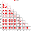 |
Fig. 6. As in Fig. 3, but for the marginalized posteriors and two-dimensional joint posteriors of the CR–M–z and M⋆, BCG–M–z relation. |
It is worth noting that Kleinebreil et al. (2025) performed a direct comparison of the weak-lensing measurements between the KiDS and HSC surveys using 48 common clusters. They found excellent agreement in the observed shear profile g+ but a significant discrepancy in the inferred excess surface mass density ΔΣm. Specifically, ΔΣm inferred from HSC is statistically higher than that from KiDS by ≈30% at a level of ≈4σ. Meanwhile, only marginal difference (at a level of ≈2.3σ) was seen in g+ and ΔΣm between DES and KiDS. Because the source redshift is required to derive ΔΣm from the observed g+, the agreement in g+ but not in ΔΣm between the KiDS and HSC surveys implies a potential systematic uncertainty existing in the source photo-z calibration. Recall that g+ ≈ γ+ = ΔΣm/Σcrit ∝ ΔΣm × β, where β is the lensing efficiency, which monotonically increases with source redshift. The higher ΔΣm in the HSC survey compared to KiDS suggests that the photo-z of the source sample is underestimated in HSC and/or overestimated in KiDS. However, the photo-z in the HSC survey is rigorously calibrated against spectroscopic samples and shows no bias at redshift z ≲ 1.2 (Rau et al. 2023). In addition, the agreement between the DES and KiDS surveys suggests no significant bias in the photo-z calibration of their source samples, which are primarily at relatively low redshift (z ≲ 1). A possible cause is that the photo-z of the HSC source sample at high redshift z ≳ 1.2 is biased low. This aligns well with the finding of the HSC-Y3 cosmic-shear analyses (Li et al. 2023; Dalal et al. 2023; Sugiyama et al. 2023), which suggest that the photo-z of the HSC sources at z ≳ 1.2 is biased low by ≈0.2 at a level of ≈2σ. However, the photo-z bias at z ≳ 1.2 at a level of ≈0.2 alone cannot explain the ≈30% difference in Σm for the eRASS1 clusters, which are primarily at redshift z ≈ 0.35. A detailed investigation of this systematic uncertainty is beyond the scope of this paper and is clearly warranty in future work, with a focus on the photo-z calibration at high redshift z ≳ 1.2.
We provide the mean of the mass posterior,  , and its sampled mass in Table B.1. The mass posterior is calculated as P(M|CR,𝒪,p), where 𝒪 = {g+,M⋆, BCG}, {M⋆, BCG}, or {g+}, depending on the data availability.
5.2. The M⋆, BCG–M–z relation
To begin with, we verify that further including the modelling of the BCG stellar mass relation, as in Eq. (21), yields a consistent CR–M–z relation. This is clearly evident from the excellent agreement between the blue (WL only) and red (WL+BCG) contours in Fig. 3, suggesting that the cluster mass estimates, informed by the X-ray count rate with an absolute weak-lensing calibration, are robust to constrain the BCG stellar mass relation.
As listed in Table 2, we obtain the constraints on the M⋆, BCG–M–z relation, i.e. Eq. (8), as
![Mathematical equation: $$ \begin{aligned} A_{\mathrm{BCG} }&= 11.547^{+0.083}_{-0.074} \, \nonumber \\[1.5pt] B_{\mathrm{BCG} }&= 0.184^{+0.068}_{-0.16} \,\nonumber \\[1.5pt] \delta _{\mathrm{BCG} }&= 0.22\pm 0.29 \, \\ \gamma _{\mathrm{BCG} }&= 1.49^{+0.88}_{-0.75} \, \nonumber \\[1.5pt] \sigma _{\mathrm{BCG} }&= 0.554^{+0.040}_{-0.049} \, .\nonumber \end{aligned} $$](/articles/aa/full_html/2025/12/aa54942-25/aa54942-25-eq91.gif) (23)
(23)
The parameter marginalized posteriors and two-dimensional joint posteriors are presented in Fig. 6 (see the full results in Appendix C). Meanwhile, we constrain the correlated intrinsic scatter as ρWL, X = −0.04 ± 0.43,  , and
, and  , suggesting no significant intrinsic correlation among the BCG stellar mass, X-ray count rate, and the weak-lensing mass at a fixed halo mass.
It is noticeable that there exists large intrinsic scatter in the BCG stellar mass M⋆, BCG at a fixed halo mass, constrained as  in this work. This corresponds to an intrinsic scatter of ≈0.24 ± 0.02 dex in a unit of log(M⋆, BCG/M⊙), which is consistent with previous studies (e.g. Leauthaud et al. 2012; Kravtsov et al. 2018; Erfanianfar et al. 2019; Akino et al. 2022). Unlike the CR–M–z relation, the M⋆, BCG–M–z relation has a shallow mass slope (
 ), so that the scatter
  in the logarithmic of the halo mass at a fixed BCG stellar mass is at a level of ≈σBCG/BBCG ≈ 3, corresponding to nearly a factor of exp(3) ≈ 20 in the halo mass M. That is, it is not feasible to adopt the BCG stellar mass as a precise mass proxy on a per-cluster basis.
Interestingly, Golden-Marx et al. (2022) found that the intrinsic scatter σBCG of the BCG stellar mass at a fixed halo mass could be largely reduced by accounting for their local environments, as indicated by the magnitude gap between the BCG and the fourth brightest cluster galaxy (see also Golden-Marx & Miller 2018, 2019). Moreover, Golden-Marx et al. (2025) measured a non-zero correlation between the magnitude gap and the central stellar mass (BCG+ICL), supporting a scenario in which BCGs primarily assemble their masses at late times through ex situ processes, such as merging. A similar correlation between the central stellar mass and the halo concentration was also found in Zu et al. (2022). Therefore, it is possible to adopt the BCG stellar mass M⋆, BCG as a reliable mass proxy for eROSITA clusters if the formation history of BCGs is properly taken into account (e.g. Huang et al. 2022).
In Fig. 7 we present the mass and redshift trends of the M⋆, BCG–M–z relation in the left and right panels, respectively, with the re-normalization as similarly done in Fig. 5. Additionally, we plot the running inverse-variance-weighted means and the standard deviations of the measurements as the pink circles, using five sub-sample bins of equal cluster numbers. As seen, the best-fit model provides a good description of the data with the noticeably large intrinsic scatter at a fixed halo mass. Our results suggest no or mildly increasing redshift trend of the BCG stellar mass at a fixed halo mass ( ) at a level of ≈2σ. However, it is in contrast to the physical picture of the hierarchical structure formation, where galaxies at late time are expected to be more massive that those at earlier time, on average (see e.g. Moster et al. 2013). This is primarily caused by the strong degeneracy between the parameters BBCG and γBCG (see Fig. 6), which arises from a combination of the large intrinsic scatter σBCG and the X-ray selection of the cluster sample. While the X-ray selection favors high-mass clusters at high redshift, the excessively large scatter σBCG (corresponding to an ≈80% variation in M⋆, BCG at a fixed halo mass M) prevents us from distinguishing between two scenarios: (1) BCGs at a fixed halo mass are intrinsically increasing with redshift or (2) more massive BCGs at high redshift appear in the sample purely due to the selection bias (i.e. the Malmquist bias; Malmquist 1922). In the absence of low-mass clusters at high redshift, it is challenging to simultaneously constrain both the mass and redshift trends given the size of the current sample.
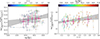 |
Fig. 7. As in Fig. 5, but for the M⋆, BCG–M–z relation of the eRASS1 clusters and the best-fit model in Eq. (23) with its fully marginalized uncertainties (grey shaded regions). We also plot the running inverse-variance-weighted means and standard deviations as the pink open circles, using five bins of an equal number of clusters. |
In light of the strong degeneracy between BBCG and γBCG, we additionally constrain the M⋆, BCG–M–z relation with an informative prior applied to the parameter γBCG. The informative prior is derived as follows. Based on Moster et al. (2013), where the authors used an abundance-match method and accounted for the Eddington bias in the halo mass estimates, they constrained the M⋆, BCG–M–z relation across wide ranges of halo mass and redshift (see their Table 1). We take an eRASS1 cluster with the mean of its mass posterior9
 , place it at a series of equal-step redshift bins zj between 0 and 1, and calculate its corresponding BCG stellar mass
  (without the intrinsic scatter and measurement uncertainty) following the Moster et al. (2013) relation assuming that it is at each redshift zj. We then re-fit the functional form
  , which is the redshift scaling of the M⋆, BCG–M–z relation, to the BCG stellar masses
  at different redshifts zj using a χ2 minimization. This gives the best-fit power-law index γ of the redshift scaling for this eRASS1 cluster with the mass
  . We repeat the aforementioned procedure for all eRASS1 clusters, resulting a distribution of the best-fit γ which represents the distribution of the power-law indices for our eRASS1 sample at their mass scales. The distribution is obtained as a nearly Gaussian 𝒩(−0.4,0.142). This result is free from the Malmquist bias because we do not include the intrinsic scatter and measurement uncertainty in calculating
  . In the end, we apply a Gaussian prior 𝒩(−0.4,0.142) to the parameter γBCG and obtain an improved constraint on the M⋆, BCG–M–z relation as
 (24)
(24)
These results are also listed in Table 2. The mass and redshift trends of the M⋆, BCG–M–z relation with the Gaussian prior on γBCG are presented in Fig. C.2.
In Fig. 8 we present the parameter marginalized posteriors and two-dimensional joint posteriors in comparison with those without the Gaussian prior on γBCG. As seen, the constraints with (blue contours) and without (red contours) the Gaussian prior are statistically consistent with each other at a level of ≈1σ. However, the degeneracy between BBCG and γBCG is broken by including the Gaussian prior, leading to a ≈1σ steeper mass trend (BBCG = 0.38 ± 0.11) with smaller error bars. The steeper mass trend (BBCG = 0.38 ± 0.11) is also in better agreement with previous studies (e.g. Gonzalez et al. 2013; van der Burg et al. 2014; Chiu et al. 2016; Kravtsov et al. 2018; Akino et al. 2022), suggesting that our constraints based on an X-ray-selected sample could be prone to the BBCG–γBCG degeneracy. Interestingly, once the BBCG–γBCG degeneracy is broken, there exists a cross-scaling between the mass and redshift (δBCG = 0.62 ± 0.25) at a level of ≈2.5σ. This parameter was constrained as −0.085 ± 0.045 in Moster et al. (2013)10, which has an opposite trend that is inconsistent with ours at a mildly significant level (≈2.8σ). A larger sample with more low-mass clusters at high redshift will shed light on this. The interpretations of the other parameters ABCG and σBCG remain unaffected by the Gaussian prior.
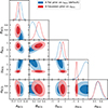 |
Fig. 8. Comparison between the M⋆, BCG–M–z relations obtained with (blue contours) and without (red contours) the Gaussian prior applied on γBCG. The Gaussian prior is obtained based on the overall mass and redshift distributions of the eRASS1 clusters studied in this work, following the assumed relation from Moster et al. (2013) (see the text for details). |
In what follows, we discuss potential systematic uncertainties arising from the SED fitting. In our fiducial analysis, we make an assumption that the BCGs are dominated by passively evolving galaxy populations, so we only fit the SPS model with the star-formation timescale τ up to 5 Gyr and low dust extinction E(B−V) = 0, 0.1, 0.2, 0.3. We examine the systematics regarding this assumption. Namely, we allow a new SPS model with τ up to 30 Gyr configured with the dust-extinction coefficient of E(B−V) = 0, 0.1, 0.2, 0.3, 0.4, 0.5 and repeat the whole analysis. We find the constraints of ABCG = 11.498 ± 0.085,  ,
,  ,
,  , and
, and  , which are in excellent agreement with the fiducial results. This reinforces the picture that the BCGs are dominated by passively evolving populations. On the other hand, we also examine the systematics due to the inclusion of the mid-infrared photometry. Specifically, we perform the SED fitting with the broadband photometry at 3.4 μm and 4.6 μm from WISE, and repeat the subsequent analysis. We obtain a result that is in agreement with our fiducial results at a level of ≲1σ, further ensuring the robustness of our SED fitting. We provide a more detailed description about the SED fitting including the WISE photometry in Appendix D.
We now turn into the comparisons of the M⋆, BCG–M–z relation with previous studies. These comparisons are illustrated in Figs. 9 and 10, which represent the trends in mass and redshift, respectively, at the pivotal values of redshift (zpiv = 0.35) and mass ( ). For the re-normalization, we adopt the best-fit parameters in Eq. (24), which are obtained with the Gaussian prior on γBCG. We note that the best-fit parameters in Eq. (24) incorporates the external information of the Gaussian prior, which is derived based on the overall mass and redshift distributions of eRASS1 clusters informed by the previous work of Moster et al. (2013). As such, our focus in this subsection is on the consistency between the eRASS1 measurements and the literature.
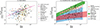 |
Fig. 9. Comparisons of the mass trend of the BCG stellar mass between the eRASS1 clusters and previous observational (left panel) and simulation-based (right panel) studies. In both panels, the mass trend is re-normalized at the pivotal redshift (zpiv = 0.35) using the best-fit M⋆, BCG–M–z relation as in Eq. (24). The eRASS1 clusters are indicated by black stars, while previous studies are shown according to the lists to the right of each panel. |
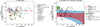 |
Fig. 10. As in Fig. 9, but for the comparisons of the redshift trend of the BCG stellar mass between the eRASS1 clusters and previous observational (left panel) and simulation-based (right panel) studies, and are re-normalized at the pivotal mass ( |

In Figs. 9 and 10, the left panels compare the results with previous observational studies, while the right panels compare them with simulation-based results. The eRASS1 cluster measurements from this work, with posterior-sampled halo masses, are indicated by black stars.
For previous observational results, we include the following:
-
Lidman et al. (2012, grey points) compiled a heterogeneous sample of clusters spanning at 0.1 ≲ z ≲ 1.6 with the halo mass estimated from either X-ray mass proxies or the line-of-sight velocity dispersion, and derived the stellar mass from the K-band luminosity.
-
Gonzalez et al. (2013, purple triangles) studied 12 X-ray-selected clusters at local Universe (z ≈ 0.1) and estimated their BCG stellar masses including the ICL.
-
van der Burg et al. (2014, red open circles) measured the BCG stellar mass using 11-band SED fitting and the halo mass from the line-of-sight velocity dispersion for a sample of high-redshift clusters (0.9 ≲ z ≲ 1.4) selected in the near-infrared.
-
Chiu et al. (2016, green crosses) studied 14 SZE-selected massive clusters at redshift 0.6 ≲ z ≲ 1.3 and derived the BCG stellar mass using SED fitting to data with wavelength from the optical to mid-infrared.
-
Kravtsov et al. (2018, brown pluses) derived the BCG stellar mass (using r-band luminosity) and the halo mass (using X-ray mass proxies) of 9 nearby clusters at z ≲ 0.1.
-
DeMaio et al. (2018, pink pluses) studied the stellar mass of BCGs and ICL for 23 clusters at redshift 0.3 ≲ z ≲ 0.9 using the imaging from Hubble Space Telescope.
-
Erfanianfar et al. (2019, yellow open circles) studied the M⋆, BCG–M–z relation of 438 X-ray-selected clusters out to z ≈ 0.65 based on the BCG stellar mass estimated from SED fitting to SDSS and WISE photometry.
-
Akino et al. (2022, red dash-dotted lines) measured the BCG stellar mass for 136 X-ray-selected clusters drawn from the XXL survey (Adami et al. 2018) using the 5-band grizY photometry from HSC.
As suggested by Chen et al. (2022, see also their detailed profile of the central stellar mass), we use the stellar mass measurements within < 50 kpc for both Kravtsov et al. (2018) and DeMaio et al. (2018) to roughly separate the BCG stellar mass M⋆, BCG from the ICL. For these comparison samples, we consistently correct for the systematics in the halo and stellar mass estimates following the prescription in Chiu et al. (2018). Specifically, the halo mass M is multiplied by 0.96 (1.12) if it is estimated from the line-of-sight velocity dispersion (X-ray mass proxies), while the stellar mass is all corrected to that inferred by the Chabrier (2003) IMF.
In the comparisons, we consider the following previous simulation-based results, including those based on the abundance-matching technique which assigns mass M from N-body simulations to observed halos statistically:
-
Both Moster et al. (2013, blue shaded regions) and Behroozi et al. (2013, red shaded regions) determined the stellar-mass-to-halo-mass relation out to high redshift z ≳ 4 using the observed stellar mass functions in the SDSS field (e.g. Baldry et al. 2008; Li & White 2009; Bouwens et al. 2012; Moustakas et al. 2013), each with a slightly different functional form.
-
Girelli et al. (2020, the cyan dotted lines) studied the stellar-mass-to-halo-mass relation in the COSMOS field using a modified functional form from Moster et al. (2013) with a focus on its redshift evolution.
All the above-mentioned studies with the abundance-matching technique assumed a fixed intrinsic scatter of the central stellar mass given a halo mass at a level ranging from ≈0.15 dex to ≈0.20 dex. The 1σ confidence regions of Moster et al. (2013) and Behroozi et al. (2013) in Figs. 9 and 10 are obtained from a full marginalization of all parameters. Meanwhile, we directly take the data points from cosmological hydrodynamic simulations (at redshift z ≲ 0.1) of
-
the IllustrisTNG simulation (Pillepich et al. 2018, green shaded regions), and
-
the Three Hundred Project (Cui et al. 2022, pink points with error bars).
No other corrections are applied to the halo mass M and the BCG stellar mass M⋆, BCG in the IllustrisTNG and Three Hundred projects in Figs. 9 and 10. We use the BCG stellar mass within 30 kpc for IllustrisTNG (Pillepich et al. 2018) due to the lack of that within 50 kpc.
As seen in the figures, the eRASS1 clusters (black stars) are in satisfactory agreement with observational results, which exhibit large scatter in M⋆, BCG at a fixed halo mass (constrained as σBCG ≈ 0.6 or ≈0.25 dex in this work). After removing the redshift dependence (γBCG ≈ −0.4) in the left panel of Fig. 9, the BCG stellar mass of the previous studies reveal a mass slope that is consistent with that of the eRASS1 sample. It is noteworthy that the eRASS1 clusters span the widest halo mass range from  to
to  , again highlighting the power of eROSITA in finding galaxy clusters and groups. Meanwhile, the agreement in the mass trend between the eRASS1 clusters and the simulation-based results is seen at a similar level (the right panel in Fig. 9). Nevertheless, we observe systematic offset in the absolute scale of the BCG stellar mass. Specifically, the BCG stellar masses from both the hydrodynamic simulations of the IllustrisTNG and Three Hundred projects are systematically higher (by a factor of ≈2 to ≈3) than eRASS1 clusters and other observational results, except for Gonzalez et al. (2013), Kravtsov et al. (2018), and DeMaio et al. (2018). On the other hand, the results from the abundance-matching method (Moster et al. 2013; Behroozi et al. 2013; Cui et al. 2022), which statistically assigns the mass M from N-body simulations to observed halos with the stellar mass estimates, are in better agreement with the eRASS1 clusters and other observational studies. This systematic difference implies possible systematics in the stellar mass produced in the hydrodynamic simulations and/or the photometric measurements in the survey pipelines (see Huang et al. 2018a; Akino et al. 2022, for details in the systematics of the cmodel photometry).
After accounting for the halo-mass dependence (BBCG ≈ 0.4) in Fig. 10, the eRASS1 measurements similarly show no significant redshift trend, in good agreement with previous studies. This finding strongly suggests that the BCG stellar mass given a fixed halo mass (i.e. the ratio M⋆, BCG/M) remains relatively stable at the high-mass end, with no clear evidence of evolution out to redshift z ≈ 1. The same picture of the little to no increase in the BCG stellar mass at the pivotal mass ( ) is also suggested by the abundance-matching results of Moster et al. (2013) and Behroozi et al. (2013). The increase of the BCG stellar mass at the pivotal halo mass from z = 0.8 to z = 0.1 is estimated to be at a level of
  , informed by the Gaussian prior from Moster et al. (2013). However, Girelli et al. (2020) reported a positive redshift trend, deviating from this pattern. Our finding is consistent with Zhang et al. (2016), where the authors obtained a mildly increasing BCG stellar mass at a fixed halo mass for X-ray-selected clusters with a scaling of ≈(1+z)−0.19 ± 0.34, corresponding to ≈0.13 dex or ≈34% from z ≈ 1 to z ≈ 0. A similar picture is also suggested by Lin et al. (2017, ≈35% increase from z ≈ 1 to z ≈ 0.3).
We note that our results quantify the scaling of the BCG stellar mass statistically as a function of the halo mass and redshift, which is complementary to the method that traces the growth of the BCG stellar mass by paring the progenitor and descendant of a cluster (see Lin et al. 2025). With a sufficiently large sample of clusters covering wide ranges of the halo mass and redshift, our approach with a flexible scaling form is expected to be equivalent to the progenitor-descendant pairing strategy. However, this is not feasible for the eRASS1 sample due to the nature of the X-ray selection, which lacks low-mass groups at high redshift that could serve as the progenitors of high-mass clusters at low redshift.
Using the merging tree in numerical simulations, Lin et al. (2013) found a significant growth of a factor ≈2.3 in the BCG stellar mass from z ≈ 1.5 to z ≈ 0.5 but no growth between z ≈ 0.5 and z ≈ 0. Similarly, Lidman et al. (2012) found a significant growth in the BCG stellar mass (after accounting the halo-mass dependence) of ≈(80±30)% from z ≈ 0.9 to z ≈ 0.1 but no growth between z ≈ 0.4 and z ≈ 0.1. This suggests that BCGs must have assembled the majority of their stellar masses at much earlier epochs (z ≳ 1), before massive clusters formed, and have accreted only small amounts at later times. Moreover, BCGs must grow primarily through an ex-situ process (e.g. merging) at late epochs, as no evidence of recent star formation is found. Consequently, the BCG stellar mass fraction (M⋆, BCG/M) exhibits a negative mass trend, i.e. BBCG − 1 ≈ −0.6, while the host cluster continues to grow significantly in the total mass M during the formation. This “rapid-then-slow” growth of the BCG stellar mass is also suggested by the semi-analytical model in De Lucia & Blaizot (2007) and further refined with an updated ICL production in Contini et al. (2014). This two-phase hierarchical formation describes that BCGs acquired their stellar masses in the core via in-situ star formation at very early epochs (z ≳ 2) and gradually assembled additional mass at the large radii via ex-situ mergers (De Lucia & Blaizot 2007; Guo et al. 2011). On the other hand, we find that BCGs at a fixed halo mass ( ) assemble little stellar mass since redshift z ≈ 0.8, which is in broad agreement with this picture of the “rapid-then-slow” mass assembly. This picture is also in line with the recent observational result in Lin et al. (2025).
6. Conclusions
Using the data from the HSC survey, we presented the weak-lensing mass calibration of 124 X-ray-selected galaxy clusters selected in the first scan (eRASS1) of the eROSITA All-Sky Survey (eRASS; Merloni et al. 2024) and constrained their BCG stellar-mass-to-halo-mass-and-redshift (M⋆, BCG–M–z) relation or the stellar-mass-to-halo-mass relation. The cluster sample spans a mass range of  and redshift range of 0.1 < z < 0.8, with the majority of low-mass systems (
 ) at redshift z ≲ 0.35.
The eRASS1 clusters were X-ray-selected (Bulbul et al. 2024) and optically confirmed (Kluge et al. 2024), leading to a clean ICM-based sample with a point-source contamination at a level of ≈5%. We used the observed X-ray count rate CR as the proxy for the halo mass (M500c or M), based on which the selection function was parametrized and evaluated at the sky location and redshift of each eRASS1 cluster (Clerc et al. 2024).
For the weak-lensing mass calibration, we measured the tangential reduced shear profile g+ of each cluster using the latest HSC-Y3 dataset (Li et al. 2022). Following the previous studies (Chiu et al. 2022, 2023), we derived the weak-lensing mass MWL and inferred the underlying halo mass M using the weak-lensing-mass-to-mass-and-redshift (MWL–M–z) relation. The MWL–M–z relation was calibrated by hydrodynamic simulations, accounting for the modelling systematics including the halo triaxiality, the miscentring of X-ray-defined centers, the cluster member contamination to the weak-lensing observable, the bias in the photometric redshift of source galaxies, the calibration uncertainty of the galaxy shape measurement, and the baryonic feedback.
For the BCG stellar mass M⋆, BCG, we employed the SED fitting technique on the grizY five-band photometry from the third Public Data Release (PDR3) of the HSC survey. The SED template was built from the model of Stellar Population Synthesis (SPS) assuming a passively evolving population, which is supported by our BCG data. We additionally examined the systematics arising from the inclusion of the mid-infrared data (from WISE) in the SED fitting and found no statistically significant change to the final results. We conclude that our BCG stellar mass estimates are homogeneous and robust. We present the HSC cutout images of these BCGs and their SED fitting results in Appendix B.
Among the 124 eRASS1 clusters in this study, 73 clusters have measurements for both the shear profile g+ and the BCG stellar mass M⋆, BCG, while 23 have only g+ measurements and 28 have only M⋆, BCG measurements. In an approach of forward and population modelling, we simultaneously constrained both the count rate-to-mass-and-redshift (CR–M–z) relation and the BCG stellar-mass-to-halo-mass (M⋆, BCG–M–z) relation, accounting for the bias and intrinsic scatter of the weak-lensing mass via the MWL–M–z relation. We also included the correlated intrinsic scatter among the X-ray count rate CR, the BCG stellar mass M⋆, BCG, and the weak-lensing mass MWL, and found no statistically significant correlation.
Using the weak-lensing shear profiles g+ alone, we obtain a constraint on the CR–M–z relation as
with the intrinsic scatter  . The resulting CR–M–z relation suggests a mass trend significantly steeper than the self-similar prediction of the X-ray luminosity-to-mass relation, but reveals no deviation from the self-similar scaling in redshift. As also found in the companion eROSITA studies (Grandis et al. 2024; Kleinebreil et al. 2025; Ghirardini et al. 2024), we confirm the excessively large intrinsic scatter σX compared to the typical value (≈0.3) obtained for the luminosity-to-mass relation in the literature. This implies that significant scatter is introduced in measuring the eROSITA observed count rate converted from the physical flux in X-rays. Our results are in good agreement with those calibrated with the weak-lensing data from the DES (Grandis et al. 2024) and KiDS (Kleinebreil et al. 2025) surveys.
The resulting M⋆, BCG–M–z relation is constrained as
 (25)
(25)
with the intrinsic scatter of  . Including the modelling of the M⋆, BCG–M–z relation has no significant impact on that of the CR–M–z relation. The intrinsic scatter of
  indicates significant variations in M⋆, BCG at a fixed halo mass M. Given the large scatter and the shallow mass slope
  , we conclude that the BCG stellar mass is a highly scattering mass proxy. Given that the X-ray selection favors high-mass clusters at high redshift, we find strong degeneracy between the power-law indices of the mass (BBCG) and redshift (γBCG) trends. To break the degeneracy, we introduced an informative prior on γBCG, which results in a steeper mass trend BBCG = 0.38 ± 0.11.
We compared our M⋆, BCG–M–z relation with both observational and simulation-based studies in the literature. We find satisfactory agreement in the intrinsic scatter and the scaling in the halo mass and redshift, though some studies exhibit systematic offsets in the absolute scale of the BCG stellar mass. However, these offsets are not significant given the large scatter and systematic uncertainties in M⋆, BCG among previous studies.
Our M⋆, BCG–M–z relation suggests that the BCG stellar mass fraction (M⋆, BCG/M) at a fixed halo mass ( ) has remained stable since redshift z ≈ 0.8, with an increase in M⋆, BCG at a level of ≈(20±8)%. As clusters continue to grow, the BCG stellar mass fraction significantly decreases with increasing total mass. This result aligns well with the picture of the rapid-then-slow BCG formation scenario suggested by previous studies (e.g. De Lucia & Blaizot 2007; Lidman et al. 2012; Lin et al. 2013). A combination of the eRASS1 sample and those sampling the low-mass regime at high redshift, possibly selected in the optical or with the planned next-generation X-ray missions (e.g. Zhang et al. 2020; Reynolds et al. 2023; Cruise et al. 2025), will shed light on the growth of the BCG mass using the statistical approach.
In summary, we presented a study of the galaxy population in the context of the BCG stellar mass based on the cluster sample constructed in the first-year database released by eROSITA-DE, paving a way for future work leveraging the final-year sample with the upcoming Stage IV experiments, such as the Rubin Observatory Legacy Survey of Space and Time (LSST Science Collaboration 2009), Euclid (Euclid Collaboration: Mellier et al. 2025), and the Nancy Grace Roman Telescope (Dore et al. 2019).
Among the 101 eRASS1 clusters, we have only 1 system with the maximum value of |ΔzBCG|≈0.066 in our sample.
The extinction laws are applied to the galaxy templates according to the prescription provided within the Le Phare package. This gives the same set of the galaxy templates used to determine the photo-z in the COSMOS field (Ilbert et al. 2009).
To the first order, this effectively assumes that the correlated scatter between 𝒮 and 𝒪 is negligible. This is a valid assumption, as the primary selection observable is the X-ray count rate CR, which is not expected to strongly correlate with the optical properties (e.g. the BCG stellar mass M⋆, BCG or the weak-lensing shear profile g+) at a fixed halo mass.
For the weak-lensing mass modelling, the relevant parameters in the vector p are (1) the miscentring parameters and (2) the cosmological parameters, which are varied with informative priors and used here to infer the angular diameter distance.
The notation of DA(z) is the angular diameter distance to the redshift z, while DA(z1,z2) represents the angular diameter distance between the redshift pairs of z1 and z2 with z2 > z1.
The extracted weak-lensing shear profile g+ shows no signature of the cluster member contamination (Chiu et al. 2022). We therefore set the cluster member contamination at a level of < 6% (2σ) at the cluster core of R ≈ 0.2 h−1 Mpc with a decaying behavior following a projected NFW profile.
The parameters δX, γX, δWL and γWL in this work correspond to the notations of FX, GX, AWL, and BWL in Ghirardini et al. (2024, and Grandis et al. 2024), respectively.
The mass posterior is calculated in Sect. 5.1 as  .
.
With the variables defined in Moster et al. (2013), the parameter γBCG can be approximated as  , where we use zpiv = 0.35 and Moster et al. (2013) obtained a constraint on γ11 as γ11 = 0.329 ± 0.173 in their Table 1.
Acknowledgments
The authors thank anonymous referee for providing useful comments that led to improvements of this paper. I-Non Chiu acknowledges the support from the National Science and Technology Council in Taiwan (Grant NSTC 111-2112-M-006-037-MY3). This work made use of the computational and storage resources in the Academic Sinica Institute of Astronomy and Astrophysics (ASIAA) and the National Center for High-Performance Computing (NCHC) in Taiwan. I-Non Chiu thanks the hospitality of Ting-Wen Lan and Ji-Jia Tang at National Taiwan University (NTU). This work was supported by JSPS KAKENHI Grant Number JP19KK0076. VG acknowledges the financial contribution from the contracts Prin-MUR 2022 supported by Next Generation EU (M4.C2.1.1, n.20227RNLY3 The concordance cosmological model: stress-tests with galaxy clusters). E. Bulbul, V. Ghirardini, A. Liu, S. Zelmer, and X. Zhang acknowledge financial support from the European Research Council (ERC) Consolidator Grant under the European Union’s Horizon 2020 research and innovation program (grant agreement CoG DarkQuest No 101002585). This work is based on data from eROSITA, the soft X-ray instrument aboard SRG, a joint Russian-German science mission supported by the Russian Space Agency (Roskosmos), in the interests of the Russian Academy of Sciences represented by its Space Research Institute (IKI), and the Deutsches Zentrum für Luft- und Raumfahrt (DLR). The SRG spacecraft was built by Lavochkin Association (NPOL) and its subcontractors, and is operated by NPOL with support from the Max Planck Institute for Extraterrestrial Physics (MPE). The development and construction of the eROSITA X-ray instrument was led by MPE, with contributions from the Dr. Karl Remeis Observatory Bamberg & ECAP (FAU Erlangen-Nuernberg), the University of Hamburg Observatory, the Leibniz Institute for Astrophysics Potsdam (AIP), and the Institute for Astronomy and Astrophysics of the University of Tübingen, with the support of DLR and the Max Planck Society. The Argelander Institute for Astronomy of the University of Bonn and the Ludwig Maximilians Universität Munich also participated in the science preparation for eROSITA. The Hyper Suprime-Cam (HSC) collaboration includes the astronomical communities of Japan and Taiwan, and Princeton University. The HSC instrumentation and software were developed by the National Astronomical Observatory of Japan (NAOJ), the Kavli Institute for the Physics and Mathematics of the Universe (Kavli IPMU), the University of Tokyo, the High Energy Accelerator Research Organization (KEK), the Academia Sinica Institute for Astronomy and Astrophysics in Taiwan (ASIAA), and Princeton University. Funding was contributed by the FIRST program from the Japanese Cabinet Office, the Ministry of Education, Culture, Sports, Science and Technology (MEXT), the Japan Society for the Promotion of Science (JSPS), Japan Science and Technology Agency (JST), the Toray Science Foundation, NAOJ, Kavli IPMU, KEK, ASIAA, and Princeton University. This paper makes use of software developed for Vera C. Rubin Observatory. We thank the Rubin Observatory for making their code available as free software at http://pipelines.lsst.io/. This paper is based on data collected at the Subaru Telescope and retrieved from the HSC data archive system, which is operated by the Subaru Telescope and Astronomy Data Center (ADC) at NAOJ. Data analysis was in part carried out with the cooperation of Center for Computational Astrophysics (CfCA), NAOJ. We are honored and grateful for the opportunity of observing the Universe from Maunakea, which has the cultural, historical and natural significance in Hawaii. The Pan-STARRS1 Surveys (PS1) and the PS1 public science archive have been made possible through contributions by the Institute for Astronomy, the University of Hawaii, the Pan-STARRS Project Office, the Max Planck Society and its participating institutes, the Max Planck Institute for Astronomy, Heidelberg, and the Max Planck Institute for Extraterrestrial Physics, Garching, The Johns Hopkins University, Durham University, the University of Edinburgh, the Queen’s University Belfast, the Harvard-Smithsonian Center for Astrophysics, the Las Cumbres Observatory Global Telescope Network Incorporated, the National Central University of Taiwan, the Space Telescope Science Institute, the National Aeronautics and Space Administration under grant No. NNX08AR22G issued through the Planetary Science Division of the NASA Science Mission Directorate, the National Science Foundation grant No. AST-1238877, the University of Maryland, Eotvos Lorand University (ELTE), the Los Alamos National Laboratory, and the Gordon and Betty Moore Foundation. This work is possible because of the efforts in the Vera C. Rubin Observatory (Juric et al. 2017; Ivezic et al. 2019) and PS1 (Chambers et al. 2016; Schlafly et al. 2012; Tonry et al. 2012; Magnier et al. 2013), and in the HSC (Aihara et al. 2018a) developments including the deep imaging of the COSMOS field (Tanaka et al. 2017), the on-site quality-assurance system (Furusawa et al. 2018), the Hyper Suprime-Cam (Miyazaki 2015; Miyazaki et al. 2018; Komiyama et al. 2018), the design of the filters (Kawanomoto et al. 2018), the data pipeline (Bosch et al. 2018), the design of bright-star masks (Coupon et al. 2018), the characterization of the photometry by the code Synpipe (Huang et al. 2018b), the photometric redshift estimation (Tanaka et al. 2018), the shear calibration (Mandelbaum et al. 2018b), and the public data releases (Aihara et al. 2018b, 2019. This work made use of the following software(s): IPython (Pérez & Granger 2007), SciPy (Virtanen et al. 2020), TOPCAT (Taylor 2005, 2006), matplotlib (Hunter 2007), Astropy (Astropy Collaboration 2013), NumPy (Van Der Walt et al. 2011), Pathos (McKerns et al. 2012), pyccl (Chisari et al. 2019), getdist (Lewis 2025), and the conda-forge project (conda-forge community 2015).
References
- Adami, C., Giles, P., Koulouridis, E., et al. 2018, A&A, 620, A5 [NASA ADS] [CrossRef] [EDP Sciences] [Google Scholar]
- Aihara, H., Arimoto, N., Armstrong, R., et al. 2018a, PASJ, 70, S4 [NASA ADS] [Google Scholar]
- Aihara, H., Armstrong, R., Bickerton, S., et al. 2018b, PASJ, 70, S8 [NASA ADS] [Google Scholar]
- Aihara, H., AlSayyad, Y., Ando, M., et al. 2019, PASJ, 71, 114 [Google Scholar]
- Akino, D., Eckert, D., Okabe, N., et al. 2022, PASJ, 74, 175 [NASA ADS] [CrossRef] [Google Scholar]
- Albareti, F. D., Allende Prieto, C., Almeida, A., et al. 2017, ApJS, 233, 25 [Google Scholar]
- Allen, S., Evrard, A., & Mantz, A. 2011, ARA&A, 49, 409 [Google Scholar]
- Applegate, D., von der Linden, A., Kelly, P., et al. 2014, MNRAS, 439, 48 [CrossRef] [Google Scholar]
- Arnouts, S., Cristiani, S., Moscardini, L., et al. 1999, MNRAS, 310, 540 [Google Scholar]
- Artis, E., Ghirardini, V., Bulbul, E., et al. 2024, A&A, 691, A301 [NASA ADS] [CrossRef] [EDP Sciences] [Google Scholar]
- Artis, E., Bulbul, E., Grandis, S., et al. 2025, A&A, 696, A5 [NASA ADS] [CrossRef] [EDP Sciences] [Google Scholar]
- Astropy Collaboration (Robitaille, T. P., et al.) 2013, A&A, 558, A33 [NASA ADS] [CrossRef] [EDP Sciences] [Google Scholar]
- Bahar, Y. E., Bulbul, E., Clerc, N., et al. 2022, A&A, 661, A7 [NASA ADS] [CrossRef] [EDP Sciences] [Google Scholar]
- Bahar, Y. E., Bulbul, E., Ghirardini, V., et al. 2024, A&A, 691, A188 [NASA ADS] [CrossRef] [EDP Sciences] [Google Scholar]
- Baldry, I. K., Glazebrook, K., & Driver, S. P. 2008, MNRAS, 388, 945 [NASA ADS] [Google Scholar]
- Bardeen, J. M., Bond, J. R., Kaiser, N., & Szalay, A. S. 1986, ApJ, 304, 15 [Google Scholar]
- Behroozi, P. S., Wechsler, R. H., Wu, H.-Y., et al. 2013, ApJ, 763, 18 [NASA ADS] [CrossRef] [Google Scholar]
- Bellagamba, F., Sereno, M., Roncarelli, M., et al. 2019, MNRAS, 484, 1598 [Google Scholar]
- Bocquet, S., Dietrich, J. P., Schrabback, T., et al. 2019, ApJ, 878, 55 [Google Scholar]
- Bocquet, S., Grandis, S., Bleem, L. E., et al. 2024a, Phys. Rev. D, 110, 083510 [NASA ADS] [CrossRef] [Google Scholar]
- Bocquet, S., Grandis, S., Bleem, L. E., et al. 2024b, Phys. Rev. D, 110, 083509 [NASA ADS] [CrossRef] [Google Scholar]
- Böhringer, H., Dolag, K., & Chon, G. 2012, A&A, 539, A120 [NASA ADS] [CrossRef] [EDP Sciences] [Google Scholar]
- Bosch, J., Armstrong, R., Bickerton, S., et al. 2018, PASJ, 70, S5 [Google Scholar]
- Bouwens, R. J., Illingworth, G. D., Oesch, P. A., et al. 2012, ApJ, 754, 83 [Google Scholar]
- Bruzual, G., & Charlot, S. 2003, MNRAS, 344, 1000 [NASA ADS] [CrossRef] [Google Scholar]
- Bulbul, E., Chiu, I. N., Mohr, J. J., et al. 2019, ApJ, 871, 50 [Google Scholar]
- Bulbul, E., Liu, A., Kluge, M., et al. 2024, A&A, 685, A106 [NASA ADS] [CrossRef] [EDP Sciences] [Google Scholar]
- Calzetti, D., Armus, L., Bohlin, R., et al. 2000, ApJ, 533, 682 [NASA ADS] [CrossRef] [Google Scholar]
- Chabrier, G. 2003, PASP, 115, 763 [Google Scholar]
- Chambers, K. C., Magnier, E. A., Metcalfe, N., et al. 2016, ArXiv e-prints [arXiv:1612.05560] [Google Scholar]
- Chen, X., Zu, Y., Shao, Z., & Shan, H. 2022, MNRAS, 514, 2692 [NASA ADS] [CrossRef] [Google Scholar]
- Chen, K.-F., Chiu, I. N., Oguri, M., et al. 2025, Open J. Astrophys., 8, 2 [Google Scholar]
- Chisari, N. E., Alonso, D., Krause, E., et al. 2019, ApJS, 242, 2 [Google Scholar]
- Chiu, I., Mohr, J., McDonald, M., et al. 2016, MNRAS, 455, 258 [NASA ADS] [CrossRef] [Google Scholar]
- Chiu, I., Mohr, J. J., McDonald, M., et al. 2018, MNRAS, 478, 3072 [Google Scholar]
- Chiu, I. N., Ghirardini, V., Liu, A., et al. 2022, A&A, 661, A11 [NASA ADS] [CrossRef] [EDP Sciences] [Google Scholar]
- Chiu, I. N., Klein, M., Mohr, J., & Bocquet, S. 2023, MNRAS, 522, 1601 [NASA ADS] [CrossRef] [Google Scholar]
- Chiu, I. N., Chen, K.-F., Oguri, M., et al. 2024, Open J. Astrophys., 7, 90 [Google Scholar]
- Clerc, N., Comparat, J., Seppi, R., et al. 2024, A&A, 687, A238 [NASA ADS] [CrossRef] [EDP Sciences] [Google Scholar]
- Comparat, J., Merloni, A., Salvato, M., et al. 2019, MNRAS, 487, 2005 [Google Scholar]
- Comparat, J., Eckert, D., Finoguenov, A., et al. 2020, The Open J. Astrophys., 3, 13 [Google Scholar]
- Conroy, C., Wechsler, R. H., & Kravtsov, A. V. 2006, ApJ, 647, 201 [Google Scholar]
- Contini, E., De Lucia, G., Villalobos, Á., & Borgani, S. 2014, MNRAS, 437, 3787 [Google Scholar]
- Costanzi, M., Rozo, E., Simet, M., et al. 2019a, MNRAS, 488, 4779 [NASA ADS] [CrossRef] [Google Scholar]
- Costanzi, M., Rozo, E., Rykoff, E. S., et al. 2019b, MNRAS, 482, 490 [CrossRef] [Google Scholar]
- Coupon, J., Arnouts, S., van Waerbeke, L., et al. 2015, MNRAS, 449, 1352 [NASA ADS] [CrossRef] [Google Scholar]
- Coupon, J., Czakon, N., Bosch, J., et al. 2018, PASJ, 70, S7 [Google Scholar]
- conda-forge community 2015, https://doi.org/10.5281/zenodo.4774216 [Google Scholar]
- Cruise, M., Guainazzi, M., Aird, J., et al. 2025, Nat. Astron., 9, 36 [Google Scholar]
- Cui, W., Dave, R., Knebe, A., et al. 2022, MNRAS, 514, 977 [NASA ADS] [CrossRef] [Google Scholar]
- Dalal, R., Li, X., Nicola, A., et al. 2023, Phys. Rev. D, 108, 123519 [CrossRef] [Google Scholar]
- De Lucia, G., & Blaizot, J. 2007, MNRAS, 375, 2 [Google Scholar]
- de Vaucouleurs, G. 1948, Ann. Astrophys., 11, 247 [Google Scholar]
- DeMaio, T., Gonzalez, A. H., Zabludoff, A., et al. 2018, MNRAS, 474, 3009 [Google Scholar]
- Diemer, B. 2018, ApJS, 239, 35 [NASA ADS] [CrossRef] [Google Scholar]
- Dietrich, J. P., Bocquet, S., Schrabback, T., et al. 2019, MNRAS, 483, 2871 [Google Scholar]
- Dore, O., Hirata, C., Wang, Y., et al. 2019, BAAS, 51, 341 [Google Scholar]
- Eddington, A. 1913, MNRAS, 73, 359 [NASA ADS] [CrossRef] [Google Scholar]
- Erfanianfar, G., Finoguenov, A., Furnell, K., et al. 2019, A&A, 631, A175 [NASA ADS] [CrossRef] [EDP Sciences] [Google Scholar]
- Euclid Collaboration (Mellier, Y., et al.) 2025, A&A, 697, A1 [Google Scholar]
- Feroz, F., Hobson, M. P., & Bridges, M. 2009, MNRAS, 398, 1601 [NASA ADS] [CrossRef] [Google Scholar]
- Furusawa, H., Koike, M., Takata, T., et al. 2018, PASJ, 70, S3 [Google Scholar]
- Garrel, C., Pierre, M., Valageas, P., et al. 2022, A&A, 663, A3 [NASA ADS] [CrossRef] [EDP Sciences] [Google Scholar]
- Ghirardini, V., Bulbul, E., Artis, E., et al. 2024, A&A, 689, A298 [NASA ADS] [CrossRef] [EDP Sciences] [Google Scholar]
- Girelli, G., Pozzetti, L., Bolzonella, M., et al. 2020, A&A, 634, A135 [NASA ADS] [CrossRef] [EDP Sciences] [Google Scholar]
- Golden-Marx, J. B., & Miller, C. J. 2018, ApJ, 860, 2 [NASA ADS] [CrossRef] [Google Scholar]
- Golden-Marx, J. B., & Miller, C. J. 2019, ApJ, 878, 14 [Google Scholar]
- Golden-Marx, J. B., Miller, C. J., Zhang, Y., et al. 2022, ApJ, 928, 28 [NASA ADS] [CrossRef] [Google Scholar]
- Golden-Marx, J. B., Zhang, Y., Ogando, R. L. C., et al. 2025, MNRAS, 538, 622 [Google Scholar]
- Gonzalez, A. H., Sivanandam, S., Zabludoff, A. I., & Zaritsky, D. 2013, ApJ, 778, 14 [Google Scholar]
- Grandis, S., Bocquet, S., Mohr, J. J., Klein, M., & Dolag, K. 2021, MNRAS, 507, 5671 [NASA ADS] [CrossRef] [Google Scholar]
- Grandis, S., Ghirardini, V., Bocquet, S., et al. 2024, A&A, 687, A178 [NASA ADS] [CrossRef] [EDP Sciences] [Google Scholar]
- Guo, Q., White, S., Boylan-Kolchin, M., et al. 2011, MNRAS, 413, 101 [Google Scholar]
- Hoekstra, H. 2003, MNRAS, 339, 1155 [NASA ADS] [CrossRef] [Google Scholar]
- Hsieh, B. C., & Yee, H. K. C. 2014, ApJ, 792, 102 [Google Scholar]
- Huang, S., Leauthaud, A., Greene, J. E., et al. 2018a, MNRAS, 475, 3348 [Google Scholar]
- Huang, S., Leauthaud, A., Murata, R., et al. 2018b, PASJ, 70, S6 [CrossRef] [Google Scholar]
- Huang, S., Leauthaud, A., Bradshaw, C., et al. 2022, MNRAS, 515, 4722 [NASA ADS] [CrossRef] [Google Scholar]
- Hunter, J. D. 2007, Comput. Sci. Eng., 9, 90 [NASA ADS] [CrossRef] [Google Scholar]
- Huterer, D., Kirkby, D., Bean, R., et al. 2015, Astropart. Phys., 63, 23 [Google Scholar]
- Ilbert, O., Arnouts, S., McCracken, H., et al. 2006, A&A, 457, 841 [NASA ADS] [CrossRef] [EDP Sciences] [Google Scholar]
- Ilbert, O., Capak, P., Salvato, M., et al. 2009, ApJ, 690, 1236 [NASA ADS] [CrossRef] [Google Scholar]
- Ivezic, Ž., Kahn, S. M., Tyson, J. A., et al. 2019, ApJ, 873, 111 [NASA ADS] [CrossRef] [Google Scholar]
- Johnston, D. E., Sheldon, E. S., Tasitsiomi, A., et al. 2007, ApJ, 656, 27 [NASA ADS] [CrossRef] [Google Scholar]
- Juric, M., Kantor, J., Lim, K. T., et al. 2017, ASP Conf. Ser., 512, 279 [NASA ADS] [Google Scholar]
- Kaiser, N., & Silk, J. 1986, Nature, 324, 529 [Google Scholar]
- Kawanomoto, S., Uraguchi, F., Komiyama, Y., et al. 2018, PASJ, 70, 66 [Google Scholar]
- Kleinebreil, F., Grandis, S., Schrabback, T., et al. 2025, A&A, 695, A216 [NASA ADS] [CrossRef] [EDP Sciences] [Google Scholar]
- Kluge, M., Comparat, J., Liu, A., et al. 2024, A&A, 688, A210 [NASA ADS] [CrossRef] [EDP Sciences] [Google Scholar]
- Komiyama, Y., Obuchi, Y., Nakaya, H., et al. 2018, PASJ, 70, S2 [Google Scholar]
- Kravtsov, A., & Borgani, S. 2012, ARA&A, 50, 353 [NASA ADS] [CrossRef] [Google Scholar]
- Kravtsov, A. V., Berlind, A. A., Wechsler, R. H., et al. 2004, ApJ, 609, 35 [Google Scholar]
- Kravtsov, A. V., Vikhlinin, A. A., & Meshcheryakov, A. V. 2018, Astron. Lett., 44, 8 [Google Scholar]
- Kuijken, K., Heymans, C., Hildebrandt, H., et al. 2015, MNRAS, 454, 3500 [Google Scholar]
- Lang, D. 2014, AJ, 147, 108 [Google Scholar]
- Lang, D., Hogg, D. W., & Schlegel, D. J. 2016, AJ, 151, 36 [Google Scholar]
- Leauthaud, A., Tinker, J., Bundy, K., et al. 2012, ApJ, 744, 159 [Google Scholar]
- Lewis, A. 2025, J. Cosmol. Astropart. Phys., 2025, 025 [Google Scholar]
- Li, C., & White, S. D. M. 2009, MNRAS, 398, 2177 [NASA ADS] [CrossRef] [Google Scholar]
- Li, X., Miyatake, H., Luo, W., et al. 2022, PASJ, 74, 421 [NASA ADS] [CrossRef] [Google Scholar]
- Li, X., Zhang, T., Sugiyama, S., et al. 2023, Phys. Rev. D, 108, 123518 [CrossRef] [Google Scholar]
- Lidman, C., Suherli, J., Muzzin, A., et al. 2012, MNRAS, 427, 550 [Google Scholar]
- Lin, Y.-T., Brodwin, M., Gonzalez, A. H., et al. 2013, ApJ, 771, 61 [Google Scholar]
- Lin, Y.-T., Hsieh, B.-C., Lin, S.-C., et al. 2017, ApJ, 851, 139 [NASA ADS] [CrossRef] [Google Scholar]
- Lin, Y. T., Chen, K. F., Chen, T. C., Chuang, C. Y., & Oguri, M. 2025, AJ, 169, 285 [Google Scholar]
- Liu, A., Bulbul, E., Ghirardini, V., et al. 2022, A&A, 661, A2 [NASA ADS] [CrossRef] [EDP Sciences] [Google Scholar]
- Liu, A., Bulbul, E., Shin, T., et al. 2024, A&A, 688, A186 [NASA ADS] [CrossRef] [EDP Sciences] [Google Scholar]
- Lovisari, L., Reiprich, T. H., & Schellenberger, G. 2015, A&A, 573, A118 [NASA ADS] [CrossRef] [EDP Sciences] [Google Scholar]
- LSST Science Collaboration (Abell, P. A., et al.) 2009, ArXiv e-prints [arXiv:0912.0201] [Google Scholar]
- Magnier, E. A., Schlafly, E., Finkbeiner, D., et al. 2013, ApJS, 205, 20 [Google Scholar]
- Malmquist, K. G. 1922, Meddelanden fran Lunds Astronomiska Observatorium Serie I, 100, 1 [Google Scholar]
- Mandelbaum, R., Lanusse, F., Leauthaud, A., et al. 2018a, MNRAS, 481, 3170 [NASA ADS] [CrossRef] [Google Scholar]
- Mandelbaum, R., Miyatake, H., Hamana, T., et al. 2018b, PASJ, 70, S25 [Google Scholar]
- Mantz, A. B., von der Linden, A., Allen, S. W., et al. 2015, MNRAS, 446, 2205 [Google Scholar]
- Mantz, A., Allen, S., Morris, R., & Schmidt, R. 2016, MNRAS, 456, 4020 [NASA ADS] [CrossRef] [Google Scholar]
- McClintock, T., Varga, T. N., Gruen, D., et al. 2019, MNRAS, 482, 1352 [Google Scholar]
- McKerns, M. M., Strand, L., Sullivan, T., Fang, A., & Aivazis, M. A. G. 2012, ArXiv e-prints [arXiv:1202.1056] [Google Scholar]
- Medezinski, E., Oguri, M., Nishizawa, A. J., et al. 2018, PASJ, 70, 30 [NASA ADS] [Google Scholar]
- Merloni, A., Predehl, P., Becker, W., et al. 2012, ArXiv e-prints [arXiv:1209.3114] [Google Scholar]
- Merloni, A., Lamer, G., Liu, T., et al. 2024, A&A, 682, A34 [NASA ADS] [CrossRef] [EDP Sciences] [Google Scholar]
- Miyatake, H., Battaglia, N., Hilton, M., et al. 2019, ApJ, 875, 63 [Google Scholar]
- Miyazaki, S. 2015, IAU General Assembly, 22, 2255916 [NASA ADS] [Google Scholar]
- Miyazaki, S., Komiyama, Y., Kawanomoto, S., et al. 2018, PASJ, 70, S1 [NASA ADS] [Google Scholar]
- Moster, B. P., Naab, T., & White, S. D. M. 2013, MNRAS, 428, 3121 [Google Scholar]
- Moustakas, J., Coil, A. L., Aird, J., et al. 2013, ApJ, 767, 50 [NASA ADS] [CrossRef] [Google Scholar]
- Murata, R., Oguri, M., Nishimichi, T., et al. 2019, PASJ, 71, 107 [CrossRef] [Google Scholar]
- Navarro, J., Frenk, C., & White, S. 1997, ApJ, 490, 493 [Google Scholar]
- Nishizawa, A. J., Hsieh, B. C., Tanaka, M., & Takata, T. 2020, ArXiv e-prints [arXiv:2003.01511] [Google Scholar]
- Oguri, M. 2014, MNRAS, 444, 147 [NASA ADS] [CrossRef] [Google Scholar]
- Okabe, N., & Smith, G. P. 2016, MNRAS, 461, 3794 [Google Scholar]
- Okabe, N., Takada, M., Umetsu, K., Futamase, T., & Smith, G. P. 2010, PASJ, 62, 811 [NASA ADS] [Google Scholar]
- Okabe, N., Reiprich, T., Grandis, S., et al. 2025, A&A, 700, A46 [NASA ADS] [CrossRef] [EDP Sciences] [Google Scholar]
- Pérez, F., & Granger, B. E. 2007, Comput. Sci. Eng., 9, 21 [Google Scholar]
- Pillepich, A., Reiprich, T. H., Porciani, C., Borm, K., & Merloni, A. 2018, MNRAS, 481, 613 [Google Scholar]
- Pratt, G., Croston, J., Arnaud, M., & Böhringer, H. 2009, A&A, 498, 361 [NASA ADS] [CrossRef] [EDP Sciences] [Google Scholar]
- Pratt, G. W., Arnaud, M., Biviano, A., et al. 2019, Space Sci. Rev., 215, 25 [Google Scholar]
- Predehl, P., Andritschke, R., Arefiev, V., et al. 2021, A&A, 647, A1 [EDP Sciences] [Google Scholar]
- Prevot, M. L., Lequeux, J., Maurice, E., Prevot, L., & Rocca-Volmerange, B. 1984, A&A, 132, 389 [Google Scholar]
- Ragagnin, A., Saro, A., Singh, P., & Dolag, K. 2021, MNRAS, 500, 5056 [Google Scholar]
- Rau, M. M., Dalal, R., Zhang, T., et al. 2023, MNRAS, 524, 5109 [NASA ADS] [CrossRef] [Google Scholar]
- Reiprich, T. H., & Böhringer, H. 2002, ApJ, 567, 716 [Google Scholar]
- Reynolds, C. S., Kara, E. A., Mushotzky, R. F., et al. 2023, SPIE Conf. Ser., 12678, 126781E [Google Scholar]
- Salvati, L., Saro, A., Bocquet, S., et al. 2022, ApJ, 934, 129 [NASA ADS] [CrossRef] [Google Scholar]
- Schellenberger, G., & Reiprich, T. H. 2017, MNRAS, 471, 1370 [Google Scholar]
- Schlafly, E. F., Finkbeiner, D. P., Jurić, M., et al. 2012, ApJ, 756, 158 [NASA ADS] [CrossRef] [Google Scholar]
- Schrabback, T., Applegate, D., Dietrich, J. P., et al. 2018, MNRAS, 474, 2635 [Google Scholar]
- Seppi, R., Comparat, J., Bulbul, E., et al. 2022, A&A, 665, A78 [NASA ADS] [CrossRef] [EDP Sciences] [Google Scholar]
- Seppi, R., Comparat, J., Ghirardini, V., et al. 2024, A&A, 686, A196 [NASA ADS] [CrossRef] [EDP Sciences] [Google Scholar]
- Shirasaki, M., Sifón, C., Miyatake, H., et al. 2024, Phys. Rev. D, 110, 103006 [Google Scholar]
- Simet, M., McClintock, T., Mandelbaum, R., et al. 2017, MNRAS, 466, 3103 [NASA ADS] [CrossRef] [Google Scholar]
- Sugiyama, S., Miyatake, H., More, S., et al. 2023, Phys. Rev. D, 108, 123521 [NASA ADS] [CrossRef] [Google Scholar]
- Sunayama, T., Park, Y., Takada, M., et al. 2020, MNRAS, 496, 4468 [CrossRef] [Google Scholar]
- Sunayama, T., Miyatake, H., Sugiyama, S., et al. 2024, Phys. Rev. D, 110, 083511 [NASA ADS] [Google Scholar]
- Sunyaev, R. A., & Zel’dovich, Y. B. 1970, Ap&SS, 7, 3 [NASA ADS] [CrossRef] [Google Scholar]
- Sunyaev, R., & Zel’dovich, Y. 1972, Comments Astrophys. Space Phys., 4, 173 [Google Scholar]
- Sunyaev, R., Arefiev, V., Babyshkin, V., et al. 2021, A&A, 656, A132 [NASA ADS] [CrossRef] [EDP Sciences] [Google Scholar]
- Tanaka, M., Hasinger, G., Silverman, J. D., et al. 2017, ArXiv e-prints [arXiv:1706.00566] [Google Scholar]
- Tanaka, M., Coupon, J., Hsieh, B.-C., et al. 2018, PASJ, 70, S9 [Google Scholar]
- Taylor, M. B. 2005, ASP Conf. Ser., 347, 29 [Google Scholar]
- Taylor, M. B. 2006, ASP Conf. Ser., 351, 666 [Google Scholar]
- The Dark Energy Survey Collaboration 2005, ArXiv e-prints [arXiv:astro-ph//0510346] [Google Scholar]
- To, C., Krause, E., Rozo, E., et al. 2021, Phys. Rev. Lett., 126, 141301 [NASA ADS] [CrossRef] [Google Scholar]
- Tonry, J. L., Stubbs, C. W., Lykke, K. R., et al. 2012, ApJ, 750, 99 [Google Scholar]
- Umetsu, K., Medezinski, E., Nonino, M., et al. 2014, ApJ, 795, 163 [NASA ADS] [CrossRef] [Google Scholar]
- Umetsu, K., Sereno, M., Lieu, M., et al. 2020, ApJ, 890, 148 [NASA ADS] [CrossRef] [Google Scholar]
- Vale, A., & Ostriker, J. P. 2004, MNRAS, 353, 189 [Google Scholar]
- van der Burg, R., Muzzin, A., Hoekstra, H., et al. 2014, A&A, 561, A79 [NASA ADS] [CrossRef] [EDP Sciences] [Google Scholar]
- Van Der Walt, S., Colbert, S. C., & Varoquaux, G. 2011, Comput. Sci. Eng., 13, 22 [Google Scholar]
- Vikhlinin, A., Kravtsov, A., Burenin, R., et al. 2009a, ApJ, 692, 1060 [CrossRef] [Google Scholar]
- Vikhlinin, A., Burenin, R., Ebeling, H., et al. 2009b, ApJ, 692, 1033 [NASA ADS] [CrossRef] [Google Scholar]
- Virtanen, P., Gommers, R., Oliphant, T. E., et al. 2020, Nat. Methods, 17, 261 [Google Scholar]
- von der Linden, A., Allen, M. T., Applegate, D. E., et al. 2014, MNRAS, 439, 2 [NASA ADS] [CrossRef] [Google Scholar]
- Weaver, J. R., Kauffmann, O. B., Ilbert, O., et al. 2022, ApJS, 258, 11 [NASA ADS] [CrossRef] [Google Scholar]
- Weinberg, D. H., Mortonson, M. J., Eisenstein, D. J., et al. 2013, Phys. Rep., 530, 87 [Google Scholar]
- Wright, E., Eisenhardt, P., Mainzer, A., et al. 2010, AJ, 140, 1868 [NASA ADS] [CrossRef] [Google Scholar]
- Zhang, Y., Miller, C., McKay, T., et al. 2016, ApJ, 816, 98 [Google Scholar]
- Zhang, C., Ramos-Ceja, M. E., Pacaud, F., & Reiprich, T. H. 2020, A&A, 642, A17 [NASA ADS] [CrossRef] [EDP Sciences] [Google Scholar]
- Zu, Y., Song, Y., Shao, Z., et al. 2022, MNRAS, 511, 1789 [Google Scholar]
- Zuntz, J., Paterno, M., Jennings, E., et al. 2015, Astron. Comput., 12, 45 [NASA ADS] [CrossRef] [Google Scholar]
Appendix A: The SQL query of the BCG photometry
In the HSC PDR3 database, we query the reliable cmodel photometry in grizY for the BCGs using the following SQL script.
SELECT
photo.object_id,
photo.ra,
photo.dec,
photo.[g,r,i,z,y]_cmodel_mag - photo.a_[g,r,i,z,y]
- offsets.[g,r,i,z,y]_mag_offset - correction.corr_[r,i]mag,
photo.[g,r,i,z,y]_cmodel_magerr
FROM pdr3_wide.forced              as photo
LEFT JOIN pdr3_wide.masks            as masks    USING (object_id)
LEFT JOIN pdr3_wide.mag_corr          as correction  USING (object_id)
LEFT JOIN pdr3_wide.stellar_sequence_offsets  as offsets   USING (skymap_id)
WHERE
photo.isprimary                  is True AND
photo.[g,r,i,z,y]_pixelflags_edge         is False AND
photo.[g,r,i,z,y]_pixelflags_interpolatedcenter  is False AND
photo.[g,r,i,z,y]_pixelflags_crcenter       is False AND
photo.[g,r,i,z,y]_pixelflags_saturatedcenter    is False AND
photo.[g,r,i,z,y]_pixelflags_suspectcenter     is False AND
photo.[g,r,i,z,y]_cmodel_flag           is False AND
masks.[g,r,i,z,y]_mask_brightstar_halo       is False AND
masks.[g,r,i,z,y]_mask_brightstar_ghost      is False AND
masks.[g,r,i,z,y]_mask_brightstar_blooming     is False AND
photo.[g,r,i,z,y]_inputcount_value         >= 2
Appendix B: The cutout images and the SED fitting of the BCGs
We provide the cutout images of the 101 eRASS1 clusters and their BCGs in Figs. B.1 to B.3. Each figure contains multiple subplots, showing the results of individual clusters in three panels: The cutout HSC images of individual eRASS1 clusters (0.5 h−1 Mpc × 0.5 h−1 Mpc) and their BCGs (15″ × 15″) are displayed in the left and middle panels, respectively. Both cutout images centre at the BCG. The grizY magnitudes (after applying all systematic corrections) and the error bars are shown in the right panel with the best-fit template. The cluster name, redshift, best-fit BCG stellar mass, and the χ2 of the best-fit template are indicated in the right panel.
In Table B.1, we provide the mass measurements of individual clusters studied in this work.
The measurements of eRASS1 clusters.
Appendix C: Auxiliary figures
We provide the following materials in this appendix. The full parameter constraints (marginalized posteriors and two-dimensional joint posteriors) of the WL-only and WL+M⋆, BCG modelling are contained in Fig. C.1. Figure C.2 shows the mass and redshift trends of the BCG stellar mass of the eRASS1 clusters, using the modelling including the Gaussian prior on γBCG (see Sect. 5.2).
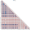 |
Fig. C.1. Same as Fig. 6, but for the full results of the parameter constraints in the WL-only modelling (blue contours) of the CR–M–z relation and the joint modelling (red lines) of the CR–M–z and M⋆, BCG–M–z relations. |
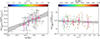 |
Fig. C.2. Same as Fig. 7, but for the result of the M⋆, BCG–M–z relation (Eq. (24)) obtained with the Gaussian prior on γBCG. |
Appendix D: The BCG stellar mass with the inclusion of the WISE photometry
The spectral energy distribution (SED) of the old stellar population in galaxies typically peaks at the wavelength range between 1μm and 2μm, while the optical emission is more subject to recent star-forming activities. Owing to the cosmological redshifting, the mid-infrared wavelength provides an excellent window with negative k-correction to probe the stellar light of the old stellar population. As BCGs are dominated by the old stellar population, the inclusion of mid-infrared photometry is expected to provide stronger constraints on the stellar mass estimates than using optical photometry alone. Independently of the fiducial analysis, we included the infrared data from the WISE all-sky survey to estimate the BCG stellar mass, and we examined the systematic uncertainty associated with the final results.
We include the mid-infrared photometry at the wavelength of 3.4μm and 4.6μm, labelled as the filters W1 and W2, respectively, from the all-sky surveys observed by the Wide-field Infrared Survey Explorer (WISE; Wright et al. 2010) to estimate the BCG stellar mass M⋆, BCG. Specifically, we use the unWISE catalogue (Lang et al. 2016) with forced photometry extracted at the location of the SDSS-DR13 sources (Albareti et al. 2017) on the unWISE coadds (Lang 2014). These coadds were reprocessed using an improved pipeline applied to the images collected in the ALLWISE (Wright et al. 2010) survey without additional blurring.
To select galaxies from the unWISE catalogue, we discard bright stars by applying the flag of pointsource! = 1 and removing objects with the W1 magnitude brighter than 14 mag. We then match the BCG catalogue of the eRASS1 clusters to the resulting unWISE catalogue to obtain the W1W2 photometry. Among the 101 clusters with the available HSC photometry for the BCGs, 96 have the W1W2 photometry from the unWISE catalogue with a median matching separation of ≈0.20 arcsec.
We re-estimate the BCG stellar mass for those 96 clusters using the seven-band photometry grizYW1W2, and re-run the subsequent analyses to derive the M⋆, BCG–M–z relation. The resulting constraints are  , which are consistent with the fiducial results (without W1W2). Therefore, we conclude that incorporating mid-infrared photometry does not have a significant impact on our final results.
For homogeneous photometric measurements, we choose not to include WISE photometry in our fiducial analyses.
All Tables
All Figures
|
Fig. 1. Footprint of the HSC-Y3 weak lensing dataset (grey dots) and the sky distributions of the eRASS1 clusters together with those categorized based on the availability of weak-lensing shear profile g+ and/or the BCG stellar mass estimate M⋆, BCG. The eRASS1 clusters with available g+ are marked as blue circles (23 clusters), those with M⋆, BCG as green diamonds (28 clusters), and those with both measurements as red squares (73 clusters). The other eRASS1 clusters with neither g+ nor M⋆, BCG are shown as grey crosses, and are excluded from this study. |
| In the text | |
|
Fig. 2. Distributions of the observed count rate CR (top panel) and the BCG stellar mass M⋆, BCG (left panel) as functions of the cluster redshift for the eRASS1 clusters studied in this work. The clusters are colour-coded as in Fig. 1. We note that a clear dependence of the BCG stellar mass on the cluster redshift is revealed in the bottom panel, which arises from the X-ray selection primarily favoring massive clusters at high redshift. |
| In the text | |
|
Fig. 3. Parameter marginalized posteriors (diagonal) and two-dimensional joint posteriors (off-diagonal) from different modelling are presented. The results of the weak-lensing mass calibration alone are shown as the blue contours, while the inclusions of the modelling of the M⋆, BCG–M–z relation are indicated by the red contours. We also indicate the results from Kleinebreil et al. (2025), based on the identical cluster sample and the weak-lensing data g+, as the green contours. |
| In the text | |
|
Fig. 4. Observed shear profiles g+ (black data points) and best-fit models with fully marginalized uncertainties (grey shaded regions). The four subplots in the left panel present the stacked profiles of the subsamples defined with respect to the median values of the observed count rate (CR = 0.487) and the redshift (z = 0.27). The stacked profile of all 96 eRASS1 clusters is presented in the right panel. The numbers of the clusters in the (sub)samples and the reduced χred2 are shown in the lower left corners. In both left and right panels, the radial values (the x-axis) of the measurements are obtained with the inverse-variance weights of the clusters in the (sub)samples. |
| In the text | |
|
Fig. 5. CR–M–z relation of the eRASS1 clusters and the best-fit model in Eq. (22). Its fully marginalized uncertainties are shown as grey shaded regions. The left panel shows the mass trend normalized at the pivotal redshift zpiv = 0.35 after accounting for the redshift-dependent factors, while the right panel similarly presents the redshift scaling normalized at the pivotal mass |
| In the text | |
|
Fig. 6. As in Fig. 3, but for the marginalized posteriors and two-dimensional joint posteriors of the CR–M–z and M⋆, BCG–M–z relation. |
| In the text | |
|
Fig. 7. As in Fig. 5, but for the M⋆, BCG–M–z relation of the eRASS1 clusters and the best-fit model in Eq. (23) with its fully marginalized uncertainties (grey shaded regions). We also plot the running inverse-variance-weighted means and standard deviations as the pink open circles, using five bins of an equal number of clusters. |
| In the text | |
|
Fig. 8. Comparison between the M⋆, BCG–M–z relations obtained with (blue contours) and without (red contours) the Gaussian prior applied on γBCG. The Gaussian prior is obtained based on the overall mass and redshift distributions of the eRASS1 clusters studied in this work, following the assumed relation from Moster et al. (2013) (see the text for details). |
| In the text | |
|
Fig. 9. Comparisons of the mass trend of the BCG stellar mass between the eRASS1 clusters and previous observational (left panel) and simulation-based (right panel) studies. In both panels, the mass trend is re-normalized at the pivotal redshift (zpiv = 0.35) using the best-fit M⋆, BCG–M–z relation as in Eq. (24). The eRASS1 clusters are indicated by black stars, while previous studies are shown according to the lists to the right of each panel. |
| In the text | |
|
Fig. 10. As in Fig. 9, but for the comparisons of the redshift trend of the BCG stellar mass between the eRASS1 clusters and previous observational (left panel) and simulation-based (right panel) studies, and are re-normalized at the pivotal mass ( |
| In the text | |
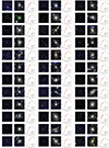 |
Fig. B.1. See Appendix B for details. |
| In the text | |
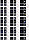 |
Fig. B.2. See Appendix B for details. |
| In the text | |
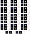 |
Fig. B.3. See Appendix B for details. |
| In the text | |
|
Fig. C.1. Same as Fig. 6, but for the full results of the parameter constraints in the WL-only modelling (blue contours) of the CR–M–z relation and the joint modelling (red lines) of the CR–M–z and M⋆, BCG–M–z relations. |
| In the text | |
|
Fig. C.2. Same as Fig. 7, but for the result of the M⋆, BCG–M–z relation (Eq. (24)) obtained with the Gaussian prior on γBCG. |
| In the text | |
Current usage metrics show cumulative count of Article Views (full-text article views including HTML views, PDF and ePub downloads, according to the available data) and Abstracts Views on Vision4Press platform.
Data correspond to usage on the plateform after 2015. The current usage metrics is available 48-96 hours after online publication and is updated daily on week days.
Initial download of the metrics may take a while.