| Issue |
A&A
Volume 704, December 2025
|
|
|---|---|---|
| Article Number | A16 | |
| Number of page(s) | 21 | |
| Section | Catalogs and data | |
| DOI | https://doi.org/10.1051/0004-6361/202555271 | |
| Published online | 28 November 2025 | |
Harnessing the XMM-Newton data: X-ray spectral modelling of 4XMM-DR11 detections and 4XMM-DR11s sources
1
INAF-Osservatorio Astronomico di Roma,
via Frascati 33,
00040
Monteporzio Catone,
Italy
2
Department of Physics, University of Helsinki,
PO Box 64,
00014
Helsinki,
Finland
3
Instituto de Física de Cantabria (CSIC-Universidad de Cantabria),
Avenida de los Castros,
39005
Santander,
Spain
4
Juelich Supercomputing Centre,
Forschungszentrum Juelich GmbH,
52425
Juelich,
Germany
5
Institute for Astronomy Astrophysics Space Applications and Remote Sensing (IAASARS), National Observatory of Athens,
Ioannou Metaxa & Vasileos Pavlou,
Penteli
15236,
Greece
6
Université Paris Saclay and Université Paris Cité, CEA, CNRS,
AIM,
91191
Gif-sur-Yvette,
France
7
Max-Planck-Institut für extraterrestrische Physik,
Giessenbachstraße 1,
Garching
85748,
Germany
8
Université de Strasbourg, CNRS, Observatoire astronomique de Strasbourg,
UMR 7550,
Strasbourg
67000,
France
9
Institut de Ciències del Cosmos (ICCUB), Universitat de Barcelona (UB), c. Martí i Franquès,
1,
08028
Barcelona,
Spain
10
Departament de Fîsica Quàntica i Astrofísica (FQA), Universitat de Barcelona (UB), c. Martì i Franquès,
1,
08028
Barcelona,
Spain
11
Institut d’Estudis Espacials de Catalunya (IEEC),
c/ Esteve Terradas, 1, Edifici RDIT, Despatx 212, Campus del Baix Llobregat UPC – Parc Mediterrani de la Tecnologia,
08860
Castelldefels,
Spain
12
IRAP, Université de Toulouse,
CNRS, UPS, CNES, 9 Avenue du Colonel Roche, BP 44346,
31028
Toulouse Cedex 4,
France
★ Corresponding author: This email address is being protected from spambots. You need JavaScript enabled to view it.
Received:
23
April
2025
Accepted:
24
September
2025
Abstract
The XMM-Newton X-ray observatory has played a prominent role in astrophysics, conducting precise and thorough observations of the X-ray sky for the past two decades. The most recent iteration of the XMM-Newton catalogue, 4XMM, and one of its latest data releases (DRs), DR11, mark significant improvements over previous XMM-Newton catalogues, serving as a cornerstone for comprehending the diverse inhabitants of the X-ray sky. In this investigation, we employ X-ray detections and spectra extracted from the 4XMM-DR11 catalogue, subjecting them to fitting procedures using simple models. Our study operates within the framework of the XMM2ATHENA project, which focuses on developing state-of-the-art methods that exploit existing XMM-Newton data. In this study, we introduce and publicly release four catalogues containing measurements derived from X-ray spectral modelling of sources. The first catalogue encompasses outcomes obtained by fitting an absorbed power-law model to all the extracted spectra for individual detections within the 4XMM-DR11 dataset. The second catalogue presents results obtained by fitting both an absorbed power-law and an absorbed black-body model to all unique physical sources listed in the 4XMM-DR11s catalogue, which documents source detection results from overlapping XMM-Newton observations. For the third catalogue we use the five band count rates derived from the pipe line detection of X-ray sources to mimic low resolution spectra to get a rough estimate of the spectral shape (absorbed power law) of all 4XMMDR11 detections. In the fourth catalogue, we conducted spectral analyses for the subset of identified sources with extracted spectra, employing various models based on their classification into categories such as active galactic nuclei (AGNs), stars, X-ray binaries, and cataclysmic variables. Finally, the scientific potential of these catalogues is highlighted by discussing the capabilities of optical and mid-infrared colours for selecting absorbed AGNs.
Key words: astronomical databases: miscellaneous / catalogs / surveys / X-rays: general
© The Authors 2025
 Open Access article, published by EDP Sciences, under the terms of the Creative Commons Attribution License (https://creativecommons.org/licenses/by/4.0), which permits unrestricted use, distribution, and reproduction in any medium, provided the original work is properly cited.
This article is published in open access under the Subscribe to Open model. This email address is being protected from spambots. You need JavaScript enabled to view it. to support open access publication.
1 Introduction
The study of X-rays from celestial sources opens a gateway to a realm of high-energy astrophysical phenomena, enabling us to delve into the nature of some of the Universe’s most extreme and time-variable objects. The XMM-Newton X-ray observatory (Jansen et al. 2001) is a cornerstone mission of the European Space Agency (ESA) Cosmic Vision programme. With its large field of view (about 30 arcmin diameter), a point spread function (PSF) with a full width at half maximum (FWHM) of ∼6′′ and a half-energy width (HEW) of ∼15′′, along with a large collecting area of 4500 cm2 at 1 keV (the largest of all current missions), it is an ideal tool for performing surveys and spectral analysis to investigate the physical properties of cosmic X-ray sources. The XMM-Newton catalogues can be considered the European counterpart to the Chandra Source Catalog (CSC), whose latest release is version 2.1 (Evans et al. 2024)1. The CSC provides high-angular-resolution source data, including spectral properties2, and complements XMM-Newton in terms of angular resolution and survey depth.
To harness XMM-Newton’s data, the XMM-Newton Survey Science Center (XMM-SSC; Watson et al. 2001), a collaboration of ten European institutes in conjunction with the XMM-Newton Science Operations Centre (SOC), has developed the Science Analysis System (SAS; Gabriel et al. 2004) software suite. The SAS enables the reduction and analysis of XMM-Newton data, supported by a dedicated pipeline for standardised processing of the science data, ultimately leading to the creation of catalogues containing information on X-ray and optical/ultraviolet (UV) sources (Page et al. 2012; Traulsen et al. 2020; Webb et al. 2020). Catalogues serve as indispensable resources for a wide range of scientific inquiries, providing homogeneous datasets for classes of objects and unveiling previously unknown sources.
The X-ray detection catalogues created from the observation data of the three camera systems (one pn and two MOS) of the European Photon Imaging Camera (EPIC; Turner et al. 2001) have been identified as 1 XMM, 2 XMM, and 3XMM, each representing a successive iteration marked by DRs in conjunction with the catalogue number. The latest version of the XMM catalogue, 4XMM (Webb et al. 2020), and its latest DR (DR11 at the time of starting this work) incorporates many improvements with respect to previous XMM-Newton catalogues and serves as a cornerstone for understanding the X-ray sky’s diverse inhabitants. The 4XMM-DR11 catalogue represents the culmination of over two decades of meticulous X-ray observations by XMM-Newton.
In this study, we utilise the X-ray detections and spectra extracted from the 4XMM-DR11 catalogue, and the unique X-ray sources from the 4XMM-DR11s catalogue, and subject them to automated fitting procedures employing both simple and physically motivated models. Our investigation is carried out within the framework of the XMM2ATHENA (Webb et al. 2023) project, which is dedicated to developing novel methodologies for harnessing the existing XMM-Newton data and preparing for its seamless integration with forthcoming NewAthena observations. In particular, we focus on automated X-ray spectral fitting pipelines and catalogue-level modelling approaches that enable population-wide analysis across millions of detections. This endeavor encompasses the incorporation of multi-wavelength and multi-messenger data, providing a comprehensive approach to unravelling the intricate cosmic phenomena captured by these advanced observatories. Specifically, we aim to reveal the X-ray spectral properties of different classes of X-ray sources, such as AGNs, X-ray binaries (XRBs), cataclysmic variables (CVs), and stars.
Direct antecedents for this work are XMMFITCAT Corral et al. (2015) and XMMFITCAT-Z Ruiz et al. (2021) (R21), which provided spectral fits for more than 114 000 detections from 3XMM-DR4 and 22 677 identified sources from 3XMM-DR6 (mostly AGNs), respectively. With respect to them, we are using later versions of the XMM-Newton catalogues with more detections and sources, and hence also more extracted spectra, and updated identifications and photometric redshifts. On the other hand, we are using a reduced set of spectral models, and fits in a single spectral band. More detailed discussions of the differences are included in Sects. 2.2.1 for XMMFITCAT and 2.2.4 for XMMFITCAT-Z.
The paper is organised as follows: Sect. 2 offers a concise overview of the 4XMM-DR11 catalogues and outlines the sources encompassed in the four catalogues we generated. Sect. 3 provides insights into the spectral models employed to fit X-ray spectra in each of the four catalogues, along with details on source classification and photometric redshift calculation. In Sect. 4, we present measurements of the primary properties of the sources and conduct a comparative analysis across the four catalogues. Sect. 5 showcases a scientific application utilizing one of the generated catalogues. Finally, Sect. 6 summarises the key findings of this study.
2 Description of the parent and generated catalogues
In this section, we provide a brief description of the parent catalogues we used in our analysis. We also describe in detail the four catalogues we compiled.
2.1 The parent catalogues
The X-ray sources utilised in our analysis were extracted from the 4XMM-DR11 catalogue (Webb et al. 2020), which is based on 12 210 XMM-Newton European Photon Imaging Camera (EPIC) observations and contains 895 415 detections surpassing a statistical detection likelihood threshold of six. These correspond to 602 543 unique sources, approximately 19% of which have more than one detection. The catalogue includes both point-like and extended sources, with extent parameters considered reliable up to a maximum extent of 80′′. The median fluxes in the total (0.2−12 keV), soft (0.5−2 keV), and hard (2−12 keV) bands are ∼2.3 × 10⁻¹⁴, 5.2 × 10⁻¹⁵, and 1.2 × 10⁻¹⁴ erg cm−2 s−1, respectively, with 16th and 84th percentile ranges of [∼5 ×.10−15, ∼8 × 10⁻¹⁴],[∼1.4 × 10⁻¹⁵, ∼2.1 × 10⁻¹⁴], and [∼3.2 × 10⁻¹⁵, ∼4.1 × 10⁻¹⁴]. Spectra are extracted for detections with more than 100 EPIC net counts in the 0.2−12 keV band (see Traulsen et al. 2020; Webb et al. 2020 for details on extraction, background modelling, and the treatment of extended emission). For these detections, one spectrum per available camera (pn, MOS1, and MOS2) were extracted from the source region (including source and background counts) and from a nearby region devoid of sources (including only background counts: see Webb et al. 2020, for details). We refer to the first as the source spectra and to the second as the background spectra.
An additional independent catalogue, termed 4XMM-DR11s (“s” denoting stacked), has been concurrently compiled by the XMM-Newton Survey Science Center (SSC). This catalogue provides a record of source detection from 8274 overlapping XMM-Newton observations. The 4XMM-DR11s contains 1488 stacks. To achieve simultaneous source detection on these overlapping observations, individual events were adjusted in position based on the outcomes of the preceding catcorr positional correction applied to the entire image during the processing of 4XMM-DR11. This adjustment resulted in a noticeable enhancement in the positional accuracy when conducting stacked source detection. All sources identified through stacked source detection are documented in 4XMM-DR11s, including those originating from image areas where only a single observation contributes. It is worth noting that there may be disparities between the same sources listed in 4XMM-DR11 and DR11s, as their input event lists are treated differently: in DR11s, stacked source detection is performed after correcting and combining multiple overlapping observations, which can lead to improved source positions, refined source parameters (e.g., extent, flux), and in some cases, detection of fainter sources not visible in individual observations (Traulsen et al. 2020). The stacked catalogue includes 358 809 sources, of which 275 440 have several contributing observations.
In the context of this paper we would like to emphasise the differences between detections, sources, and stacked sources: the same physical source can give rise to several detections in 4XMM-DR11, one for each time XMM-Newton pointed in its direction. Each of these detections is represented by a unique detection identifier DETID. Within 4XMM-DR11 the unique physical sources have been determined, assigning to each one of them a unique source identifier SRCID, so several detections can have the same source identifier. On the other hand, each entry in the stacked catalogue 4XMM-DR11s corresponds to a unique physical source, with their unique identifier also named SRCID. Their correspondence with the 4XMM-DR11 sources and detections (when found) is included in the stacked catalogue in additional rows, containing their detections and source identifications as DETID_4XMMDR11 and SRCID_4XMMDR11, respectively.
2.2 Description of the compiled catalogues
We generated four catalogues using the 4XMM-DR11 and 4XMM-DR11s parent catalogues. Below is an overview of these datasets.
2.2.1 Modelling the extracted spectra of 4XMM-DR11
In the first catalogue (C1 hereafter), we present the results from fitting an absorbed power-law model (detailed in the next section) to all extracted spectra in the 4XMM-DR11. We furnished the parameter values that yield the best fit as well as their associated confidence intervals. To expedite the execution of spectral fits, we merged all source and background spectra from the same detection and camera within the same observation using the SAS task epicspeccombine. This approach ensures that, for each detection, we ended up with a maximum of one pn spectrum and one MOS spectrum.
For the spectral fitting and modelling procedures, we employed the analysis software Sherpa 4.9.1 (Freeman et al. 2001) and the Bayesian X-ray Analysis (BXA) tool (Buchner et al. 2014). The BXA tool facilitates the connection between Xspec (Arnaud 1996) and the nested sampling package UltraNest (Buchner et al. 2021). We assigned uninformative priors to each parameter within the model and explored the entire parameter space using equal-weighted sampling points, conducted via the MLFriends algorithm (Buchner 2019), which is integrated within UltraNest.
We perform spectral fitting using the Cash statistic (C-stat; Cash 1979), which is well suited for Poisson-distributed data, especially in the low-count regime. The fitting procedure is as follows: first, we merged the spectra of all exposures for the same EPIC camera type (pn and MOS) using the SAS task epicspeccombine, resulting in a maximum of one pn and one MOS spectrum for each detection. Second, the background spectra for each camera (pn and MOS) are grouped to ensure a minimum of one count per bin. These background spectra are then fit using an empirical model tailored to each camera (see Sect. 3.1). Fits with probabilities p<0.01 are rejected and not used for further analysis. These p-values (pval_bg_pn, pval_bg_mos) are reported in our catalogues, and the det_use flag depends on their outcome.
Then, we bin the source+background spectra similarly (≥ 1 count per bin), preserving the Poisson nature of the data. Finally, we fit the combined spectra for both cameras with a source+background model, where the background model parameters (except the normalisation) are fixed to the best-fit values obtained in the first step. This ensures consistency and prevents overfitting. For background spectra, the typical number of bins per camera ranges from 20 to 60, depending on the exposure and source brightness, with more than 90% of cases having at least ten bins. Background spectra with zero counts are excluded from the analysis.
Although joint fitting of the source and background spectra with all components free is often preferred for propagating uncertainties, we opted to model the background separately and fix its shape during the source+background fit. This decision was motivated by the complexity of the empirical XMM-Newton background, which includes numerous components with many free parameters, and by the need to ensure robust convergence in a fully automated pipeline. By fitting the background first, we allow better control over the model components and avoid degeneracies with the source model (see e.g. Buchner et al. 2014).
Out of the 895 415 detections listed in the 4XMM-DR11 catalogue, 319 565 of them, originating from a total of 11 907 observations, contain significant count numbers that qualify them for automated spectral extraction within the processing pipeline (Webb et al. 2023). For 390 detections (∼0.1%) the automated definition of a background extraction region of at least one camera failed and the resulting background spectrum has no counts. If we also demand that a detection has more than zero net counts in each contributing camera (pn and/or MOS)3 a further 4435 detections (∼1.5%) are excluded. This results in 314 352 detections that constitute what we call the “Good sample”. Out of these detections, 245 484 (∼80%) gave an acceptable fit for the background model (i.e., χ2 p-value >0.01, see Sect. 3.1) and 232 816 (73.8%) of them also gave an acceptable fit for the source model. These sources comprise, what we call the “Good-fit sample” (see Table 1). Among these, 100 237 detections (making up 43.1%) are present in both cameras, 135 342 detections (constituting 58.2%) exclusively stem from the pn camera, and 73 986 detections (representing 31.8%) solely arise from the MOS camera.
Corral et al. (2015) in XMMFITCAT provided fit results for over 114 000 detections, corresponding to ∼78 000 unique sources, using three bands (soft 0.5−2 keV, hard 2−10 keV, and full 0.5−10 keV) and six spectral models (three simple and three more complex ones, the latter only applied to sources with more than 500 counts). They used the default Xspec algorithm (Levenberg-Marquardt) to find the best-fit values for each model parameter, with some optimisations included in their scripts to compensate for its tendency to find local rather than global minima. We provide fit results for 319 565 detections, corresponding to 213 154 unique sources, using BXA, which makes a thorough search of the parameter space using UltraNest, making it much better suited to find global minima. While they fitted the background-subtracted spectrum using C-stat, we fitted first the background file using BXA and an empirical model, and then we fitted the source+background spectrum with the background model parameter values fixed to the best-fit background-only values, apart from the normalisation. A further refinement is that our goodness of fit (GoF) calculation accounts for the fact that the data and the simulations used to estimate the GoF are not independent, which is not taken into account using goodness within Xspec, as they did. On the other hand, the sheer number of fits constrained us to use a single band (0.2−12 keV) and a single model (an absorbed power law, also included in XMMFITCAT).
Number of detections (C1, C3) or sources (C2, C4) included in each one of the four compiled catalogues.
2.2.2 Modelling the stacked spectra of 4XMM-DR11s
In the second catalogue that we release (C2 hereafter), we fitted both an absorbed power-law model and an absorbed black-body model to sources from the 4XMM-DR11s catalogue. Using two models for the full set of 4XMM-DR11 detections (see C1 above) was not feasible due to the significantly larger number of sources involved and the associated computational cost.
The 4XMM-DR11s catalogue contains 60 720 unique sources associated with 135 612 detections with extracted spectra. Among these, 27 640 sources are associated with only a single detection. For such sources, an absorbed power-law model has already been applied in C1, where individual detections were modeled. Since the aim of C2 is to exploit the additional information from multiple detections by stacking them, we do not re-fit sources with only one detection in this catalogue. These sources therefore remain part of C1 only, and are not included in C2. This ensures that the added complexity of C2, including model comparison and stacked spectra, is applied only to cases where multi-epoch data provides additional value.
Following a methodology similar to that used in the case of C1, we excluded detections where at least one camera’s background spectrum contained no counts or where the net counts in at least one camera were less than zero. For the remaining sources with just one contributing detection after this step, we already possess spectral information from C1. Consequently, a total of 458 sources were omitted from C2, leaving us with 32 622 remaining sources. For these, we computed the signal-to-noise ratio (S/N) for each individual detection (by summing the counts from pn and MOS in the full band). We then sorted the detections in descending order of S/N and calculated a cumulative S/N (cS/N) for each detection, incorporating all detections with an equal or higher S/N. Combining spectra from multiple observations results in an average spectrum that represents the time-averaged source properties. This approach is appropriate for most sources, especially given that our spectral models are relatively simple and are not designed to capture detailed spectral evolution. While strong variability could introduce complexities in interpreting the averaged parameters, the stacked spectrum remains a valid representation of the source’s mean behavior over the combined epochs.
Out of the 19 081 sources with only two contributing detections, we used both detections if the cS/N increased when including the second, lower S/N spectrum (this was the case for 16 959 sources). In contrast, for the remaining 2122 sources, only the first detection was considered, as their spectral properties are already covered by analysis followed for the first catalogue (i.e., C1) and, therefore, not included in this part. We also excluded 173 sources from C2 for which the detection with the highest individual S/N coincided with the highest cS/N, as only one spectrum would contribute.
For the sources with more than two contributing detections (13 541−173 = 13 368 sources), we introduced a selection criterion based on the relative range (rr) of the cS/N to optimise the number of observations that are included in the spectral fitting. This relative range is calculated as the difference between the cS/N and the maximum individual value, divided by the average of the individual values:
 (1)
(1)
Our aim was to identify the detection where the cS/N reached its maximum or where adding further detections did not improve it significantly anymore. Especially in the latter case, it is better to use the relative rather than the absolute range, as we can then define a negligible increase by a fixed value that is applicable to all sources (see below). This last detection, along with all detections possessing a higher individual S/N than this last one, would be included in our spectral analysis of the source.
To address situations where there might be some “flickering” in the cS/N, we imposed a limit of >0.001 for the increase in the relative cS/N. In other words, if the change in relative cS/N between the new detection and the previous one (with a higher individual S/N) was ≤ 0.001, the new detection would not be included in the stacked spectrum. In two cases, only one detection remained after this procedure, and consequently, these two sources were also excluded from our study.
After implementing the aforementioned process, we were left with 30 325 sources with at least two contributing detections, which we again refer to as the Good sample (the average number of spectra used for the final stacked spectrum per source is three, with contributions from 2−44 spectra). We merged the spectra of all contributing detections for the same camera using the SAS task epicspeccombine, resulting in a maximum of one pn and one MOS spectrum for each source. Specifically, 19 973 sources had spectra in both cameras, 7311 sources were solely observed with the pn camera, and 3041 sources were exclusively obtained from the MOS cameras. Out of the 30 325 sources, the number that meet the requirements described in the previous section and are included in the Good-fit samples are, 23 426 that were fitted with a power-law model and 15 352 with the black-body model.
2.2.3 Modelling the count rates of 4XMM-DR11
As part of the detection process for each observation, count rates are determined for each XMM-Newton camera in the five standard bands. The standard bands 1−5 correspond to energies 0.2−0.5 keV, 0.5−1 keV, 1−2 keV, 2−4.5 keV, and 4.5−12 keV, respectively.
We used these detection count rates from the 4XMM-DR11 catalogue to build X-ray spectra for the 895 415 detections included in the catalogue. Using the count rates in the five defined energy bands for each EPIC camera, along with proper Redistribution Matrix Files (RMFs) and Auxiliary Response Files (ARFs), we obtained a set of data equivalent to very low resolution X-ray spectra. In other words, this technique is roughly equivalent to extracting an X-ray spectrum and grouping it into five bins corresponding to the 4XMM energy bands. These spectra can be fitted in the same way as the spectra in the previous sections. The results of this analysis are given in our third catalogue (C3 hereafter). Using this method we are able to give at least a crude estimate for the spectral parameters of all sources in the 4XMM-DR11, even in those cases where, given the low number of counts, a proper X-ray spectrum was not extracted.
For each of these low resolution spectra, we used as RMF the canned matrix calculated by the XMM-Newton calibration team for the corresponding camera, epoch, and mode of the observation4. As ARF matrices we calculated a set of matrices using the arfgen SAS tool, one per camera and filter (Thin, Medium, or Thick). We took into account that the count rates are already corrected for vignetting, camera efficiency, PSF losses, bad pixels and charge-coupled device (CCD) gaps, so none of these effects are included in the ARF generation. The count rates are background-subtracted, so no background spectra are needed. In this case, the MOS spectra were not merged.
In our case the likelihood probability is estimated through the χ2 value for a set of model parameters (log L=−χ2/2). By construction our count rate spectra are binned, background subtracted X-ray spectra, so no other statistic, more suited for Poisson-distributed data (e.g., Cash 1979), can be employed. Note also that for sources with very low count rates some of the bins in our spectra have less than 20 counts, and therefore a χ2 statistic is not correct from a statistical point of view (Cash 1979). Hence, be aware that our procedure only gives a quick, rough estimate of the posterior distribution of the spectral parameters. For more rigorous results, a proper X-ray spectral modelling should be done. In those cases where the source is included in the C1 or C2 catalogues, we strongly recommend using those results.
We fitted the 895 415 detections included in the 4XMMDR11 catalogue, obtaining an acceptable fit for 89.7% of them. Since we did not include any filtering in our selection, the catalogue can include a non negligible number of spurious sources, detections in problematic fields or with other observational issues. We defined a “Clean sample” by selecting detections with SUM_FLAG ≤ 1, OBS_CLASS ≤ 3 and EP_8_DET_ML ≥ 10. Moreover, the spectral model we selected is reasonably flexible for AGNs, but not so well suited for other X-ray populations, like clusters, hot stars, neutron stars, XRBs, etc. In order to minimise the non-AGN contamination in the Clean sample, we also included only sources with EP_EXTENT_ML ≤ 1 and above the Galactic plane (|b|>20°), where the bulk of the stellar population is concentrated. Thus 419 118 detections remain within this Clean sample, while 95.5% of them are included in the Good-fit sample.
2.2.4 Modelling the classified sources of 4XMM-DR11/DR11s
In the fourth catalogue (C4), we performed spectral fitting for the spectra of sources with available classification from the Tranin et al. (2022) sample, as described in Sect. 3.3. To generate this catalogue, we needed to merge the C1 and C2 catalogues, avoiding multiple appearances of the same physical source. We started by excluding from C1 all the DETID associated with the SRCID_4XMMDR11 included in C2. The remaining detections from C1 were appended to the stacked sources in C2 to generate a merged catalogue with the desired properties. For sources with multiple DETIDs linked to the same SRCID_DR11, we calculated the S/N using the source and background counts in the spectrum and sorted them in descending order. The detection with the highest S/N was selected. The outcome of this initial step was utilised to add the SRCID_DR11 associations to each spectrum in C2. Finally, the results of the last two steps were concatenated, resulting in a total of 210 444 sources. Among these, 180 118 and 30 326 are sourced from C1 and C2, respectively.
Then, we conducted a cross-match between our dataset and Tranin et al. (2022) using sky coordinates and a matching radius of 1′′. This was necessary because the sources in that study were obtained from 4XMM-DR10 and the SRCID do not have a continuity between releases of the catalogue (although most of them match). The number of detections/sources with extracted/merged spectra with classifications from Tranin et al. (2022) ultimately amounted to 92 238, with 76 610 of them being AGNs. From this AGN subset, we selected those with AGN probability ≥ 95%, as calculated by Tranin et al. (2022), and with Galactic latitudes |b|>20°. This criterion yielded 35 538 AGNs. Out of these, 8467 had spectroscopic redshifts, and the rest had photometric redshifts, as explained in Sect. 3.4.
The C4 includes 51 166 sources in total. The distribution by classification is as follows: 35 538 AGNs, 14 308 stars, 1091 XRBs, and 229 CVs. Among these sources, 24 402, 5579, and 21 185 have been detected exclusively in pn, MOS, or both pn and MOS, respectively. Applying the same criteria described in the previous sections, we ended up with 50 956 sources in the Good sample. Out of these sources, 41 142 meet the requirements and are included in the Good-fit sample. Of these, 30 814 of them are classified as AGNs, 9353 as stars, 883 as XRBs and 92 as CVs.
In R21, spectral fitting results are included in the 0.5–10 keV band for 30 816 source detections, corresponding to 22 677 unique sources, while C4 includes fits to 35 538 unique AGNs in the 0.2−12 keV band. Compared to XMMFITCAT, XMMFITCAT-Z used BXA for improved sampling of the parameter space, as we did, but they used the wstat implementation of C-stat in Sherpa. wstat approximates background modelling by assigning one free parameter per background bin. This approach can lead to biased estimates5. In contrast, we used an empirical background model, fitted to the background spectrum and then fixed (apart from the normalisation) in the source+background fit. They fitted two simple and two more complex models to their AGNs, while we fitted only one, an intrinsically absorbed power law, in common with them. We both used a similar method for the GoF. A comparison with their results on the search for absorbed sources is given in Sect. 5.
2.3 Summary of fitting approaches across the four catalogues
To aid comparison across the four catalogues, we briefly summarise the key methodological aspects here. Catalogues C1, C2, and C4 share a common spectral fitting framework: spectra are binned to a minimum of one count per bin, background and source+background models are fitted using C-stat (Cash 1979), and the background is treated via an empirical model whose parameters (except normalisation) are fixed in the final fit. Catalogue C3 differs in that it uses count rates in five predefined energy bands to construct low-resolution spectra, which are modeled using χ2 statistics.
C1 includes all 4XMM-DR11 detections with ≥ 100 net counts, fitted with an absorbed power law. C2 focuses on stacked spectra from 4XMM-DR11s sources with multiple detections, using both absorbed power-law and black-body models. C4 applies the same fitting methodology as C1 and C2 but uses classification information to assign appropriate models (see Sect. 3.5). The background fitting criteria, GoF thresholds, and model priors are consistent across C1, C2, and C4.
3 Overview of the spectral models, source classification and calculation of photometric redshifts
In this section, we describe the models used for the X-ray spectral fitting of the sources in each one of the four catalogues we complied. We also explain how we classified the sources included in C4 and calculated their photometric redshifts.
3.1 Background model fitting
For the background model used for the fitting of the spectra, we employed the XMM-Newton empirical background model integrated into the bxa.sherpa.background module (Buchner et al. 2014). This model is composed of two main components: one addressing the cosmic X-ray background and X-ray emissions from the local hot bubble and Galactic halo, and another component focused on modelling the camera background, including line contributions. Importantly, the latter component is not subjected to the instrumental response.
The background model is a combination of empirical components, including power laws, Gaussian lines, and thermal emission, inspired by the approach described in Maggi et al. (2014). It is fitted through a multi-step process designed to handle the large number of free parameters and to adapt flexibly to different camera configurations and background conditions. To verify the robustness of this model, we performed tests in which the number of free parameters was reduced by using a simplified background model. These tests were applied to a representative subsample of sources and showed that the derived source parameters (e.g., photon index and intrinsic absorption) were consistent with those obtained using the full background model, with differences well within the statistical uncertainties and following a one-to-one correlation. These results confirm that the empirical background model used within BXA adequately captures the background structure without introducing significant biases in the source spectral parameters.
To evaluate GoF for the background spectra, we used a procedure based on approximating C-stat with a chi-square distribution, since C-stat does not provide a direct measure of GoF. All background spectra were fitted using C-stat in the Poisson regime with BXA, but to compute p-values we followed a twostep procedure. First, we determined the effective number of free parameters for the pn and MOS cameras, acknowledging that not all background model components were required in every case. To do this, we used a subset of spectra with at least 1000 background counts and binned into 30 energy bins over the 0.2− 12 keV range. We then compared the resulting C-stat values to χ2 distributions with varying degrees of freedom to infer the effective number of parameters, finding twelve for pn and seven for MOS.
In the second step, we re-binned the background spectra to have at least 20 counts per bin (reducing to ten in rare cases of low background), and calculated p-values by comparing the observed χ2 values (obtained after re-binning) to the corresponding chi-square distribution using the effective number of parameters. Although admittedly ten counts per bin is on the low side, we point out that almost always the sources in the Good-fit sample (see below) have more than 100 counts in both their background and source+background spectra, effectively comparable to spectra binned at 20 counts, a more usual binning size. In cases where the number of bins was too small to allow a statistically meaningful p-value (i.e., fewer bins than the effective number of free parameters), we reduced the number of effective parameters accordingly to ensure a valid degrees-of-freedom estimate. Detections requiring such adjustments were flagged and excluded from the Good-fit sample. A p-value threshold of 0.01 was applied to define the Good-fit sample. We emphasise that this procedure was used solely for flagging based on the background fit quality; all spectral fits themselves were carried out using C-stat.
For the purpose of assessing the quality of the fit, a χ2 p value of ≥ 0.01 was considered acceptable. In cases where the spectra were available in both cameras and the χ2 p-value in one camera fell below this limit while the other exceeded it, only the source spectrum of the latter camera was taken into consideration.
3.2 Source spectral models for C1, C2, and C3
We employed an absorbed power-law model as the source model for C1, C2, and C3. To determine the flux within the 0.2− 12 keV range, we incorporated the cflux model in Xspec: cflux * tbabs * powerlaw. In instances where the object is observed by both cameras, we introduced an inter-instrument normalisation (IIN) constant defined as MOS/pn, using the const model in Xspec. Although an absorbed power law is the model of choice for AGNs (see below), for the limited resolution of CCD X-ray spectra with moderate spectral quality, it is sufficiently flexible to provide a reasonable result for most sources. The parameters left unconstrained include the logarithm of the neutral hydrogen column density of the absorber log (NH/cm−2), allowed to vary between 20 and 26, the power-law photon index Γ, which varies between 0 and 6, the logarithm of the flux in the 0.2−12 keV band log (fX/erg cm−2 s−1) varying between −17 and −7, and the IIN constrained between 0 and 5. BXA necessitates the specification of a probability prior for each free parameter in the model, and we opted for flat priors for all four parameters in the intervals above.
In addition, for C2 we also fitted an absorbed black body (cflux * tbabs * bbody in Xspec), which could provide a better fit for Galactic sources. With respect to the parameters and ranges given above for the absorbed power law, the only changes are the adjustment of the log (NH/cm−2) lower limit from 20 to 18, and the replacement of the photon index by the black-body temperature k T, allowed to vary between 0.01 and 10 keV, also with a flat prior.
Since we have used C-stat for the fits and a large fraction of the spectra have less than 100 net counts, we have decided not to use χ2 as a GoF indicator. The maximum likelihood C-stat lacks a direct estimate of GoF. Therefore, we used the method proposed by Buchner et al. (2014), also followed in R21. We calculated the Kolmogorov-Smirnov (KS) statistic between the observed and expected data+model counts, and the corresponding p-value, as a quantitative estimate of the GoF. However, we note that in this case the p-values for the KS statistic cannot be calculated the usual way. The cumulative distribution of the model depends on the parameters that were estimated from the data distribution. This implies that the two compared distributions are not independent. Nevertheless, we can do a permutation test to get an estimate of the p-value. For each source, we did 1000 resamplings, rearranging the original data+model sample in two equal-size subsamples, where the counts in each energy bin can come either from the data or the model sample, and estimate the corresponding KS statistic. Our estimated p-values are the fraction of resamplings that have statistics larger than the statistic of the original samples. Any model showing a KS p ≥ 0.01 is considered as an acceptable fit.
While several studies (e.g., Buchner et al. 2014; Marchesi et al. 2016; Masini et al. 2020; Liu et al. 2022; Peca et al. 2023; Boorman et al. 2025) have highlighted the importance of including a soft X-ray component in AGN spectral models, such as scattered power-law emission or thermal excess, our present work adopts a simpler approach using a single absorbed power law. This choice was motivated by the limited photon statistics in many of our sources, the need to maintain a manageable number of free parameters in automated fits, and a uniform approach over the full catalogue. We acknowledge that the lack of a soft component can introduce biases in the estimation of spectral parameters, particularly for obscured sources. A future extension of this work will explore multi-component models in a subset of well-exposed AGNs to quantify this effect.
We note that the spectral model used for C3 contain at most four free parameters: normalisation, photon index, absorption, and the IIN (the latter parameter is free only if spectra from both types of EPIC camera are used in the fit). Given that the spectra consist of five coarse flux bins across XMM bands, this ensures that the number of free parameters does not exceed the number of data points (N=5), preserving statistical robustness.
For all catalogues the mode and median values of each calculated parameter are provided, along with the narrowest interval that includes 90% of the probability, and percentiles of 5 and 95 per cent. Throughout this paper, we use the mode values of the presented parameters.
3.3 Source classification
To categorise the X-ray sources included in C4, a probabilistic technique using a naive Bayes classifier was devised, which is thoroughly explained in Tranin et al. (2022). In essence, this approach drew inspiration from its intuitive characteristics, extending from the basic classification principles seen in rudimentary decision trees. To carry out the classification of X-ray sources, specific data columns from the XMM-Newton catalogue’s 4XMM-DR10 version were employed.
The catalogue was also expanded with multi-wavelength counterparts, employing the NWAY algorithm (Salvato et al. 2018) and using a number of available catalogues (e.g., Gaia, GLADE) as described in Tranin et al. (2022). A dataset of 25 160 previously identified sources was generated and categorised into distinct subgroups, encompassing AGNs, stars, XRBs, and CVs. The probability density for various properties associated with each source type was estimated and these probabilities were utilised to assess the likelihood of classifying the sources. In cases where a property value was missing, the likelihood was substituted with the probability that a source of that class would have a missing value for that property. Subsequently, Bayes’ rule was applied, considering each property for each source type, to determine the probability associated with the source’s nature. Additionally, an outlier class was introduced to identify rare sources of other types. The algorithm’s performance was validated using a test sample, yielding outstanding precision results: 97.2% for AGNs, 98.9% for stars, 93.7% for XRBs, and 84.6% for CVs (Tranin et al. 2022).
3.4 Photometric redshifts
For the X-ray sources classified as AGNs, based on the source classification method outlined in the previous sub-section, we performed the computation of photometric redshifts. To achieve this, we employed the methodology detailed in Ruiz et al. (2018). In a nutshell, this approach leverages optical counterparts from datasets like SDSS or PanSTARRS for the X-ray sources and, whenever feasible, also seeks counterparts in the near-infrared (NIR; e.g., 2MASS, UKIDSS, VISTA-VHS) and/or mid-infrared (MIR; AllWISE).
To facilitate the cross-correlation of multiple catalogues, we utilised the xmatch tool from the astromatch package6. This tool facilitated the matching of multiple catalogues and provided Bayesian probabilities for associations or non-associations, as detailed in Pineau et al. (2017); Ruiz et al. (2018). Subsequently, a machine-learning (ML) technique was applied to compute photometric redshifts. Specifically, we employed the MLZ-TPZ method, as described in Carrasco Kind & Brunner (2013), which relies on a supervised technique involving prediction trees and random forest. MLZ-TPZ is a Python package that can be executed in parallel, enabling the swift and reliable calculation of photometric redshifts along with their corresponding probability distribution function (PDF).
The cross-matches and the photometric redshifts were based on preliminary results from XMM2ATHENA at the time this work was done, and are available from the authors upon request. The final catalogues are available in the project web pages and will be fully presented in Nebot et al. (in prep.) and Ruiz et al., (in prep.), respectively.
This preliminary catalogue of photometric redshift was built using the training sample presented by Mountrichas et al. (2017) and Ruiz et al. (2018); it contains ∼5000 X-ray selected AGNs with optical counterparts in SDSS or PanSTARRS and reliable spectroscopic redshifts. More than 90 per cent of the training sources have additional photometry in the near-infrared (NIR) and/or mid-infrared (MIR).
The statistical accuracy and reliability of our photometric redshift was estimated through the widely used normalised median absolute deviation (NMAD) σNMAD and the percentage of catastrophic outliers η7. For sources with SDSS (PanSTARRS) photometry, η ranges from 9 (4) per cent for extended sources with additional photometry in the NIR and MIR to 29 (41) per cent for point-like sources (i.e., optical emission dominated by the AGN) with photometric information only in the optical bands. Changes in σNMAD are less significant depending on the optical morphology and the amount of photometric information, ranging from ∼0.08 in the worst case (only optical photometry) to ∼0.04 in the best case (full photometry in the optical and IR bands). For a detailed analysis of this crossvalidation and potential explanations for the differences between SDSS and PanSTARRS results, see Ruiz et al. (2018). We note that in this work, we use only the best-fit point estimates of the photometric redshifts in the spectral fitting.
3.5 Source spectral models for C4
For sources in the C4 catalogue, different models were used, based on the classification of the sources, as described in the following sections. The number of sources in each category, including the Good and Good-fit samples are listed previously in Sect. 2.2.4.
3.5.1 Active galactic nuclei
For AGNs, a redshifted absorbed power-law model with Galactic absorption was utilised, the local Galactic absorption with NH fixed to the total NH in that line of sight, plus in-situ absorption at the AGN redshift with free NH. Specifically, the model employed is cflux * tbabs(ztbabs * zpowerlaw) and we utilise the same priors for the parameters as in Cl (Sect. 3.2). The power law is thought to arise from upscattering of photons from a hot corona, while the absorption is associated with an obscuring circumnuclear structure (the torus). We fix the value of the redshift to zbest, which is either the spectroscopic redshift (when available) or the mode of the photometric redshift PDF (zmode0). About 8500 redshifts are spectroscopic.
3.5.2 Stars
For stars, we fit a single Astrophysical Plasma Emission Code (APEC) plasma (Dere et al. 1997; Smith et al. 2001). APEC models the X-ray emission arising from the stellar corona. The corona is a region of highly ionised gas surrounding a star, characterised by high temperatures (typically millions of degrees Kelvin). This hot plasma emits X-rays which are modeled by the APEC model. APEC incorporates various physical parameters of the plasma, such as temperature, elemental abundances, and emission measure, to calculate the expected X-ray spectrum. In Xspec notation the model reads cflux * tbabs * apec. We utilise the same priors as in the C2 absorbed black-body model (Sect. 3.2), but modify slightly the upper limit of the APEC plasma temperature k T to vary between 0.01 and 17 keV.
3.5.3 X-ray binaries
The XRBs are binary star systems in which the accretion process from a compact object, such as a neutron star or a black hole, from their companion normal star, can produce intense X-ray emission. The X-ray spectra of XRBs are typically modeled using a black-body and a power-law component.
In the case of neutron stars, the black-body component in XRB spectra represents thermal emission from a hot surface, where the black-body temperature is related to the surface temperature of the neutron star. For black holes, which have no surface, the thermal emission is often modeled using a disk black-body component to represent the accretion disk’s emission. It is important to note that the black-body results differ from the typical disk black-body ones.
The power-law component in XRB spectra is associated with non-thermal processes, often related to the corona surrounding the compact object. The power-law index characterises the shape of the non-thermal emission spectrum. High-energy processes, such as inverse Compton scattering, can contribute to the power-law component. While the accretion disk emits thermal emission, it also reflects Comptonised photons, which are not directly related to the disk itself.
In Xspec, the joint black-body and power-law model reads cfluxbb * tbabs * bbody +cfluxpl * tbabs * powerlaw, where the two components of the flux refer to the two separate model components, and the tbabs is the same between the two flux components. We adopt the same priors for the parameters as in C1 and C2 (Sect. 3.2), while allowing log (NH/cm−2) to vary between 18 and 24.
3.5.4 Cataclysmic variables
The CVs are binary star systems consisting of a white dwarf primary star and an usually main-sequence secondary star. The white dwarf accretes matter from its companion, leading to various types of outbursts and transient phenomena. CVs are characterised by their erratic behavior and can undergo episodes of increased brightness, such as dwarf novae outbursts or classical novae explosions.
X-ray emission from CVs is often associated with the accretion process. As matter from the secondary star accretes onto the white dwarf, it forms an accretion disk, and the release of gravitational potential energy results in high-temperature regions that emit X-rays. One common process responsible for X-ray emission in CVs is bremsstrahlung. Bremsstrahlung occurs when charged particles, such as electrons, are deflected by the strong electric fields in the vicinity of other charged particles, causing them to emit radiation. In the context of CVs, the hot plasma in the accretion disk emits X-rays through bremsstrahlung. In Xspec notation the bremsstrahlung model reads cflux * tbabs * bremss. We utilise the same priors as in the C2 black-body model (Sect. 3.2), but allow the bremsstrahlung plasma temperature k T to vary between 0.0001 and 200 keV.
4 Results
In this section, we describe the main properties calculated by following the analysis we applied on the four catalogues, as described in Sect. 2.2. In all cases, the measurements from the Good-fit subsets of each catalogue is presented.
4.1 Main properties of sources included in C1
As previously mentioned, the C1 catalogue includes the results from fitting an absorbed power-law model to all extracted spectra of detections in the 4XMM-DR11 dataset (Sect. 2.2.1). The top-left panel of Fig. 1 presents the distribution of the p-values of the fits for the sources included in the Good-fit sample of C1, as indicated in the legend. The top-right panel presents the distribution of the fluxes of the sources. As previously mentioned, fluxes are obtained in the 0.2−12 keV band, by including the cflux component in our model. In case of multiple camera spectra for a detection, the reported flux is the pn flux. The median value of the mode calculations of the flux is log (fX/erg cm−2 s−1) = −13.44, with a scatter (standard deviation) of 0.6 (Table 2). The scatter is estimated by first computing the differences between individual flux values and the median flux. The standard deviation of these differences is then calculated to quantify the typical dispersion of values around the median, providing a measure of statistical scatter.
The middle left and right panels of Fig. 1 present the measurements for the spectral parameters, namely the hydrogen column density NH and photon index Γ, respectively. The median values (of the mode calculations) are log (NH/cm−2)=21.26 and Γ=1.95. We notice a second lower tail in the Γ distribution at very high values (∼6). This is probably caused by trying to fit thermal emission with an absorbed power law. There is also a peak at log (NH/cm−2) ≈ 20. We note that these extreme values close to the chosen limits of the priors should be treated as lower or upper limits of their respective parameters (see Sect. 3). A cross-match of our dataset with the SIMBAD database (Wenger et al. 2000) reveals that this peak is mainly populated by stars.
The bottom-left panel of Fig. 1 presents the IIN, defined as MOS over pn. The median value of the (mode) IIN is 1.05. Previous measurements of the XMM-Newton IIN range from 1.02-1.08 based on 2XMM (Read et al. 2014), and ∼1.04−1.17 for 3C273 and PKS 2155-304 (Madsen et al. 2017). Our values are consistent with these measurements especially so given the broad distribution in IIN. About 1% of the sources (4 052) present an IIN above two or below 0.5. This can be explained by the fact, that if two MOS cameras are present then their spectra were combined. This merging included cases where the combined spectra are taken in two different camera submodes. In addition, the submodes between the pn and MOS cameras may also differ. We checked the relative contribution to the overall and the extreme cases for the different camera submode combinations. A significantly enhanced contribution to the extreme cases is only found for observations where any pn submode is combined with the ‘Fast (Un)compressed’ mode of one or both MOS. However, this cannot explain the number of sources we get with very high or low IIN values, as there are only a few detections with this combination of submodes (0.7% of the detections in the Good-fit sample that have pn and MOS spectra).
These results may be directly compared to the Chandra Source Catalog (CSC) 2.1 (Evans et al. 2020), where a similar approach of fitting an absorbed power law to detected sources is employed. Their master source table contains 407 806 unique sources from 15 533 Chandra observations. The total area is 730 deg2, which decreases to 705 deg2 and 137 deg2 at fluxes fainter than <10−13 and <10−15 (in any Chandra band), respectively. We select 86 368 sources at >5 σ flux significance and culling flagged sources. The corresponding CSC 2.1 power-law model median, 16th, and 84th percentiles are  and
and  , which are in agreement with our reported values within the errors.
Median values of (the mode of) each parameter for each source in the catalogues C1-4.
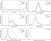 |
Fig. 1 Distributions of the p-values (top-left panel), flux (top-right panel), NH (middle-left panel), photon index (middle-right panel), IIN (bottomleft panel) and black-body temperature (bottom-right panel) of the sources included in the Good-fit samples of C1, C2, and C3, as indicated in the legends. |
4.2 Main properties of sources included in C2
The C2 catalogue, includes the results of fitting an absorbed power-law model and an absorbed black-body model to the merged spectra of all sources of the 4XMM-DR11s catalogue with more than one contributing observation (see Sect. 2.2.2). Fig. 1 displays the distributions of the p-values, fX, NH, IIN, Γ and the black-body temperature of the two Good-fit samples, as indicated in the legend. The median values of the mode calculations, for the power-law and the black-body models, respectively, are: log (fX/erg cm−2 s−1) = −13.43 and −13.80, log (NH/cm−2)=21.04 and 19.06, IIN = 1.08 and 1.10, respectively (Table 2). The median values of the photon index, calculated for the power-law model is 1.91 and the median black-body temperature is 0.40 keV. About the black-body temperature, we note that there are some sources with extreme k T values up to 9.7 keV. However, less than one per cent (88 sources) have k T values higher than 3 keV.
About five per cent of the sources have IIN above 2 or below 0.5, independent of the source model. This fraction is lower with increased count rate, and is stronger for the black body than for the power law. We also note that this fraction is higher in C2 compared to C1. For C2, we do not only combine spectra of the two MOS cameras and fit spectra of different pn and MOS submodes simultaneously, but we also combine spectra of different observations. This can be a reason for the higher percentage of extreme cases and the reduced dependence on count rate.
Regarding the spectral parameters, the distribution of the photon index parameter calculated for the power-law model, similarly to the C1 catalogue, presents a second, lower peak at high Γ values. As mentioned earlier, this could be due to trying to fit thermal emission with an absorbed power law.
A comparison between the fluxes and IIN values calculated using the power-law and black-body models reveals strong agreement between the two approaches. However, the power-law model generally produces higher flux estimates than the blackbody model. This difference likely arises because most X-ray sources are expected to be AGNs, for which an absorbed power law typically provides a more accurate representation than a black body (see Appendix A.1).
4.3 Main properties of the detections included in C3
As mentioned earlier, the C3 catalogue includes the results of the fitting of the spectra, constructed using the count rates in five energy bands, from the 4XMM-DR11 catalogue. Fig. 1 presents the distributions of the various parameters calculated by fitting the Good-fit sample of C3, as indicated in the legend. The median value of log (fX/erg cm−2 s−1)=−13.74 (Table 2). The median value of the neutral hydrogen column density is log (NH/cm−2)=21.28 and the median value of photon index is Γ=2.03 that is close to the expected value for a population dominated by AGNs (≈ 2; Nandra & Pounds 1994), and similar to the Γ values obtained for the C1 and C2 catalogues (Table 2). There is also a non-negligible number of sources in the extremes of our selected photon-index interval. The spectral model we used is probably not adequate for these ultra-hard/ultra-soft sources. The median values of IIN is 1.08, suggesting the possible inaccuracies in the cross-calibration of XMM-Newton cameras are small.
In the subsections about catalogues C1 and C2, the merging of MOS spectra and the combination of observations were mentioned as reasons why extreme IIN values are obtained. However, none of these cases apply to C3. It was also stated that combining different submodes of pn and MOS can only explain a small fraction of those cases. Therefore, previous sections do not fully account for why extreme values of IIN are observed in C3. In C3, the extreme IIN values are more likely due to the limitations and simplifications of the spectral models used, as well as potential issues with the data quality or the presence of peculiar sources that are not well-represented by the applied models.
To evaluate the differences between using count rate spectra (C3) and applying proper spectral fitting (C1), we compare the calculated values for fX, NH, Γ, and IIN between the C3 and C1 catalogues (see Appendix A.2). Our findings indicate that fX values from the two methods are in good agreement, with mean and median differences of 0.05 and 0.02, and a scatter of 0.24. Correlations for NH and Γ are also reasonable but with larger scatter, mainly due to poorly constrained posteriors in low-count sources. IIN values generally cluster around one, though the correlation is weaker, especially in the C1 catalogue, where MOS spectra were merged. These results support the use of count rate spectra for population studies, provided proper filtering is applied, while detailed spectral fitting remains preferable for individual sources.
4.4 Main properties of sources included in C4
The C4 catalogue, as mentioned in Sect. 2.2.4, includes spectral fitting for sources identified as AGNs, XRBs, CVs and stars. Fig. 2, presents the distributions of the p-values, fX, NH, IIN, k T and Γ calculated by fitting the best-fit subsets of C4 with the four models corresponding to their respective classifications. The median values of the mode of each parameter are shown in Table 2. For the sources identified as AGNs, the intrinsic (i.e., absorption corrected) rest-frame 2−10 keV luminosity LX has been computed using the chains of flux and Γ measurements obtained from the X-ray spectral fitting process, and we provide the mode and the narrowest interval that encompasses 90% of the values. The AGNs in our dataset have a median log (LX /. erg s.−1) ≈ 44.
We find overall strong agreement in fX, IIN, and Γ measurements between catalogues, with mean and median differences close to zero and moderate scatter. Comparisons between C4 and C1/C2 confirm the consistency of spectral parameters, especially for AGNs. For XRBs, fX values are systematically higher in C4 due to model differences, while IIN shows good agreement. A significant correlation between flux and p-value differences supports the improved fit of the more complex model in C4. For more details see Appendix A.3.
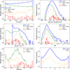 |
Fig. 2 Distributions of the p-values (top-left panel), flux (top-right panel), NH (middle-left panel), IIN (middle-right panel), black-body temperature (bottom-left panel) and photon index (bottom-right panel) of the sources included in the Good-fit sample of C4. Blue lines present the results for AGNs (zpltb model), green lines display the measurements for stars (APEC model), orange lines show the calculations for XRBs (bbpl model) and red lines illustrate the results for CVs (bremss model). |
5 Science application
We show in this section one of the potential applications of these catalogues. We use C4 to assess the optical/MIR colour AGN selection techniques, in particular their capabilities to select X-ray selected absorbed AGNs, along the lines of R21. With respect to that work, we have a larger number of unique sources and we discuss the effects of different thresholds and definitions of absorbed and unabsorbed sources.
This section is only intended to showcase the scientific potential of the catalogues. We did not attempt to address the multiple selection effects in the C4 catalogue. Sensitivity limits for each band and observation/stack are available in the XMM-Newton Science Archive (XSA) and stacked web pages, but quantifying the consequences of using only classified sources with extracted spectra, and selecting just sources with photometry in all bands and with good photometric redshifts, is beyond the scope of this paper.
In this section we start from the C4 Good-fit sample. A further selection in the sample was to use only sources with multi-wavelength counterparts, extracted during the work for finding multi-wavelength counterparts and identifications for XMM-Newton sources within the XMM2ATHENA project. The number of sources at this stage includes 30 610 AGNs, 1525 stars, 50 XRBs and 35 CVs. The latter two types of sources are shown in some figures, but we did not take further interest in them, due to the limited statistics.
We matched the stars to the Gaia DR3 catalogue (Gaia Collaboration 2016, 2023) within 1′′ of the sky positions of the multi-wavelength counterparts, using Vizier and the CDS X-match service, getting matches for 1496 stars. One of the parameters from Gaia is the effective temperature of the stars Teff. We defined as low T and highT stars those with Teff below and above 4000 K, respectively. There are 355 lowT stars and 807 highT stars. That information is missing for 334 stars.
An X-ray luminosity limit commonly used in the literature to select AGNs is 1042 erg s−1 in the 2−10 keV band, since there are no local pure star-forming galaxies with a luminosity in that range above that limit. One of the most X-ray luminous galaxies in that category is NGC3256, with an X-ray luminosity of only 2.5 × 1041 erg s−1 but with no evidence for an AGN (Moran et al. 1999). Following R21, we selected the AGNs for which the upper 90% uncertainty limit in their luminosity is higher than 1042 erg s−1. Changing this criterion to be that the mode of the luminosity being above that limit leads to a reduction of the samples by ∼0.5−1% and does not change any of the conclusions below. Furthermore, <4% of the AGNs selected with our criterion have the lower 90% confidence limit on their luminosities below 1042 erg s−1, ensuring that the vast majority of samples have luminosities above that limit with 95% confidence. Finally, we restricted the sample to AGNs with redshifts z<3.5, to facilitate the comparison with that R21. There are 29 935 AGNs fulfilling these conditions. In the rest of this section these are called Good-fit AGNs.
R21 found a number of sources with X-ray luminosity above 1048 erg s−1, which they argued were unphysical. They therefore defined a “reliable sample” (a subsample of the Good-fit AGNs) by requiring that the photometric redshift probability was concentrated in a single peak (parameter PDF_PS ≥ 0.7) and that the 90% confidence interval in the column density was ≤ 2 dex for absorbed sources (see below). We followed that definition for ease of comparison with them, but we note here that there are no sources among the Good-fit AGNs with luminosity above that value. Finally, for their reliable sample, R21 excluded absorbed AGNs (see below for definition) with luminosities above 1045.3 erg s−1. Since there are no high luminosity sources in our sample, we did not introduce any upper cut on the luminosity to define the reliable sample. We use this definition of reliable samples in the rest of this section. The concrete numbers of AGNs in them are given below for several definitions of absorbed and unabsorbed AGNs.
Having selected a reliable sample, for our main results we define absorbed AGNs (absAGN) as those with very flat photon indices (upper limit of the 90% confidence interval on the photon index Γ<1.4) or with large column densities (lower limit of the 90% confidence interval on the column density above 1022 cm−2) and unabsorbed AGNs (unabsAGN) all the rest, as in R21. The former condition is commonly used to select X-ray absorbed samples (e.g. Corral et al. 2014), and it is based on the observation that Compton-thick sources show flat X-ray spectra when fitted with a simple power law (e.g. Matt et al. 1996). We finally have 29 935 Good-fit AGNs, 1526 of which are absorbed and 28 409 are unabsorbed. The reliable sample includes 21 999 unique AGNs, of which 1137 are absorbed and 20 862 are unabsorbed (to be compared with 977 and 17 158 reliable absorbed and unabsorbed detections in R21). We examine the effects of this definition on our conclusions in two ways: first by changing the limit for absorbed sources to log (NH/cm−2)>23(log NH 23 limits: 655/29 280 absAGN/unabsAGN, 444/21 567 reliable absAGN/unabsAGN), and second keeping our default limit on the column density, but defining unabsorbed sources as those with the upper limit of the 90% confidence interval below that limit, the rest being undetermined AGNs (undetAGN) (logNH90% limits: 1526/17 601/10 808 absAGN/unabsAGN/undetAGN, 1137/13 403/7459 reliable absAGN/unabsAGN/undetAGN). This last definition of unabsorbed AGNs is more stringent, since for them we can say, with ∼95% confidence, that the absorption is below our default limit, so they are genuinely unabsorbed (with the definition above, we just cannot tell apart these objects from e.g. those with absorption but large error bars).
In Fig. 3 we show the distributions of the redshifts and luminosities of the reliable absAGN and unabsAGN samples. The redshift distributions are significantly different (the KS p-value is essentially 0): the medians are 0.53 and 0.83, respectively, with absAGN concentrating at z<1 (>85% are below that value), while unabsAGN have a higher fraction of sources at higher z (>57% are above that value). The luminosity distributions are also significantly different (KS p-value corresponding to >6 σ) but the differences are quantitatively small, with medians of 43.82 and 43.95, respectively. The higher incidence of absorbed sources at lower redshifts may be a selection effect due to, e.g., the lower number of counts detected from absorbed sources, since then their spectra may not be extracted by the XMM-Newton pipeline. Additionally, the effect of absorption is higher at lower energies, and this range moves out of the XMM-Newton range as the redshift increases, making the effect of absorption more difficult to detect at higher z (as discussed e.g. by Marchesi et al. 2016). This feature is also seen in the top panel of Fig. 4, where the first two redshift bins are higher than the rest. Similar properties can be found using the logNH 23 absAGN definition and the more restrictive logNH 90% unabsAGN definition.
We show in Fig. 4 the fraction of absorbed sources defined as Nabs /(Nabs+Nunabs) as a function of redshift (top panel) and log luminosity (bottom panel). We estimated the error bars using the expression for the binomial distribution with high number of sources. We used Bayesian blocks (Scargle et al. 2013) to define the log luminosity bins8. As in R21 (their Fig. 6), we find no evidence of a dependence of the fraction of absorbed sources with redshift (except for the first two bins in z, probably due to selections effects, see above), also getting similar fractions and little difference between the Good-fit and reliable samples. The picture is also similar when looking for a dependence on luminosity, no significant one is found: the highest luminosity bin for the Good-fit AGN sample is higher than for the reliable sample, but compatible with it, within errors. The latter is also compatible with the lower luminosity bins. Estimating fractions with the higher threshold for the definition of absAGN, logNH 23 produces a lower fraction of absorbed sources (as expected, since the higher threshold is more stringent). The qualitative behavior of the fractions as a function of redshift and luminosity are the same. The introduction of the undetAGN category does not affect the default results, since the fraction of absorbed AGNs does not change.
In contrast with this constant and low fractions, other studies with similar luminosity medians and similar or higher redshifts, but correcting for the selection effects discussed at the beginning of this section and using more sophisticated spectral models (e.g. Peca et al. 2023; Vijarnwannaluk et al. 2022; Buchner et al. 2015; Signorini et al. 2023; Aird et al. 2015; Pouliasis et al. 2024), find much higher absorbed fractions ∼0.6, generally increasing with redshift and decreasing with luminosity, except for Pouliasis et al. (2024), who find a constant fraction with redshift between local (Boorman et al. 2025) samples and their redshift 3–6 sample.
Mid-infrared colours are often used for identifying AGNs. In particular, the Wide-field Infrared Survey Explorer (WISE) W1 (3.4 μm), W2 (4.6 μm), W3 (12 μm) and W4 (22 μm) bands (e.g. Stern et al. 2012; Mateos et al. 2012; Assef et al. 2013; Glikman et al. 2018). Galaxies are generally expected to exhibit bluer colours than AGNs in the MIR regime. The bottom panel of Fig. 5 shows the W1−W2 colours of our default sample. There is considerable overlap between the W1−W2 colours of absAGN and unabsAGN, and the differences in the medians are small compared to the dispersion (0.75/0.86 for absAGN/unabsAGN), consistent with the expectation that the MIR emission originates from the torus and is independent of the inclination (see Padovani et al. 2017, and references therein). The initial simple W1−W2 criterion of Stern et al. (2012) has been updated by Assef et al. (2013) introducing a dependence on the W2 magnitude. In Fig. 6, we present the W1−W2 colour distribution vs. W2 for our default reliable absAGN/unabsAGN definition, XRBs, CVs and stars with Gaia detections. We also show in that figure one such criterion, showing that it is unable to select about half the AGNs in our sample, both for the absAGN and unabsAGN, as found by R21. A similar conclusion is reached if the criterion of Assef et al. (2018) is used instead. Using the log NH 23 and log NH 90% limits also provide similar results. Our results and those of R21 are in agreement with Hickox et al. (2017), who show that luminous quasars can be effectively selected using simple MIR colour criteria, but those criteria fail for heavily obscured and lower luminosity AGNs.
Other optical and mixed optical/MIR colours are commonly used to select AGNs. The middle panel of Fig. 5 shows r−W2 for our reliable AGN sample: they are centered in similar values, but the absAGN sample is wider, with KS p-values ∼0. Yan et al. (2013) propose that r−W 2>6 allows for selecting obscured AGNs, combined with pure MIR diagnostics, arguing that the r band suffers from extinction more strongly than W2. R21 find a slight tendency for absAGN to have a stronger r−W 2>6 tail than unabsAGN, which is even weaker in our sample. Those authors offer an explanation: Hickox et al. (2017) show that the r−W2 criterion is only actually effective for z > 1, while most of our (and R21) absAGN are below that redshift. The more strict definition of absAGN using log NH 23 reduces the number of z > 1 absAGN, and thus the r−W 2>6 tail for absAGN, even more. The more stringent definition of log NH 90% produces equivalent results to those of our standard definition.
We also display in Fig. 5 (top) the distribution of g−i for our reliable AGN sample. Since the presence of X-ray absorption is often accompanied by optical obscuration, and the effect of the latter is more pronounced at optical/UV wavelengths, it is not surprising at first view that absAGN peak at redder g−i colours than unabsAGN, but the presence of a second peak in the absAGN distribution at g−i ≈ 0.3 and the significant tail with g−i > 1 for unabsAGN reveal a more complex story. As can be appreciated in Fig. 7, redshift has a strong effect on g−i: most of the g−i > 1 sources are at z<1, and most of the g−i<1 sources are at z > 1, with no clear difference between absAGN and unabsAGN in the latter redshift range. If we restrict the analysis to z<1 there is a clear preponderance of absAGN at g − i > 1, with unabsAGN more spread in the g−i range of ∼0.01 to ∼1.7. Quantitatively, the median of g−i for z<1 unabsAGN is 0.84, while >90% of absAGN in the same redshift range have g − i > 0.84. The colour g−i allows selecting absAGN only at z<1 and with a strong mixture of unabsAGN. We reach a similar conclusion with the log NH 23 limits.
Comparable results are again obtained with the more tight limits for logNH 90%: now >93% of z<1 absAGN are above the median value for genuine unabsAGN g−i = 0.71. It is interesting to note that this median is lower than for the default and log NH 23 limits, and it is plainly lower than for undetAGN, which have a median g − i = 1.25, >74% of them having g − i > 0.71. The more stringent log NH 90% limits patently make a difference in the g−i colour between undetAGN and genuine unabsAGN at z<1.
To summarise our conclusions about the use of optical, MIR or mixed optical/MIR colours to select absorbed AGNs: W1−W2 and r−W2 are not successful in separating absorbed AGNs in our samples, not even when restricting the selection to z > 1 or using higher values of the fitted column density NH to define absorbed sources. The colour g−i is a bit more successful at z<1, with absorbed AGNs having mostly g −i > 0.8−1, but with a strong contamination of unabsorbed AGNs (about half the unabsorbed AGN colours are above that limit). Similar conclusions are reached if a higher limit is used to define absorbed sources or if we take into account the uncertainties on the fitted values of NH to define unabsorbed sources.
In contrast, CVs and XRBs tend to agree with the Assef et al. (2013) criterion in Fig. 6, their MIR colours being closer to stellar than AGN, unsurprisingly. Stars tend to occupy a pair of roughly horizontal and parallel branches in this diagram, well below the AGN boundary, the top branch corresponding to low T stars and the bottom branch corresponding to highT stars. The W1−W2 colours of stars have already been discussed by Nikutta et al. (2014), who showed that main sequence stars without significant circumstellar IR excess (“naked” stars) have a range of W1−W2 colours, with Vega-like hot stars having W1−W2 ≈ 0 and cooler stars extending up to 0.2-0.3 (see their Fig. 7). The two branches disappear when the absolute W2 magnitude instead of the apparent one is plotted in the horizontal axis (using the Gaia distance), with the top branch becoming a continuation of the lower branch towards higher absolute magnitudes (lower luminosities) and higher W1−W2 colour. As stated above, the XMM-Newton spectra of the objects classified as stars were fitted with a single APEC model in C4. Given the above dependence on Gaia Teff, we checked whether there is any correlation between any of those parameters (temperature k T, flux, line of sight column density NH and Teff), finding none. This is not surprising, since X-ray emission in main sequence stars is mainly from the corona of the star, which is thought to be heated by magnetic reconnection, which is powered by a dynamo effect in the outer layers of the star, but well below the surface where the Gaia Teff is measured.
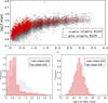 |
Fig. 3 Distribution of 2−10 keV rest-frame intrinsic luminosity LX and redshift z of the reliable AGN sample. In the top panel, the grey and red dots correspond to unabsAGN and absAGN, respectively. Note that due to the discreteness of the zmode 0 from tpz (see the text for the details), the red-shift value plotted here is offset by a random number between −0.05 and 0.05. Bottom panels show the histograms of the redshift (left) and luminosity (right) of the Good-fit and reliable absAGN and unabsAGN samples. |
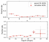 |
Fig. 4 Fraction of absorbed AGNs as a function of redshift (top) and luminosity (bottom) both for the Good-fit AGN sample (grey dots) and for the reliable AGN sample (red triangles). |
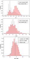 |
Fig. 5 Distribution of g−i (top), r−W2 (middle) and W1−W2 (bottom) colours of our reliable AGN samples, with absAGN in red and unabsAGN in grey. In the bottom panel we also show the simple W1−W2 colour criterion to select AGNs from Stern et al. (2005). |
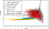 |
Fig. 6 WISE W1−W2 colour vs. W1 for reliable absAGN (red dots), unabsAGN (grey dots), XRBs (pink triangles), CVs (blue triangles), lowT stars (cyan squares), and highT stars (gold squares). The AGN locus (above the black line) of Assef et al. (2013) is also shown. |
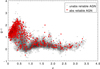 |
Fig. 7 Colour g−i vs. redshift for our reliable AGN sample: absAGN in red and unabsAGN in grey. |
6 Conclusions
In this study, we employed X-ray detections, sources, and spectra derived from the 4XMM-DR11 and 4XMM-DR11s catalogues, subjecting them to fitting procedures employing both simple and physically-motivated models. Our analysis yielded the creation of four distinct catalogues. The first catalogue (C1) utilised the 4XMM-DR11 detections, employing a simple absorbed power-law model to analyze the extracted X-ray spectra in the XMM-Newton pipeline. This provided insights into the distribution of flux, IIN, hydrogen column density (NH), and photon index (Γ). The second catalogue (C2) presented results from applying both absorbed power-law and absorbed black-body models to merged spectra from the stacked sources from the 4XMM-DR11s catalogue, providing additional information such as black-body temperature. The third catalogue (C3) uses the count rates from the source detection as low resolution spectra, fitting simple absorbed power laws to them, expanding the results of C1 to all the detections, not only those with sufficient net counts to have extracted spectra in the XMM-Newton pipeline. The fourth catalogue (C4) concentrated on AGNs, XRBs, CVs, and stars, incorporating classifications from Tranin et al. (2022) and fitting a combination of the detection spectra in C1 and the merged spectra in C2. For each class of sources a distinct physically-motivated model was fitted, allowing an easier physical interpretation of the results. The catalogue entries include median and mode values for all calculated parameters, along with the 5th and 95th percentiles and the narrowest 90 per cent interval. Throughout this work, we report results using the mode values of the parameters. The main conclusions of our analysis are summarised below:
Sources in C1 present a median flux of log (fX/erg cm−2 s−1)=−13.44, with IIN mostly around 1.05. Spectral parameters include median log (NH/cm−2)=21.26 and Γ=1.95 (probably because the catalogue source population is dominated by AGNs, which have typically similar values of their photon index). Some sources show a secondary tail in Γ at high values, likely from attempting to fit thermal emission with an absorbed power law.
In C2, absorbed power-law and absorbed black-body models provide flux measurements with a median difference of ∼0.2 dex, perhaps because the former is a better model for the majority of the sources (AGNs). There is a good agreement between the IIN distributions of the two models. Black-body temperatures generally below 3 keV are found for the majority of sources.
The fit to all detections in C3 allows extending the simple absorbed power-law modelling to all detections in 4XMMDR11, providing some spectral information from fainter sources than available in C1. The derived fluxes are compatible between the two approaches.
In C4, the results show a strong agreement in flux measurements with C1 for AGNs, stars, XRBs and CVs. The IIN and Γ comparisons between C1 and C4 exhibit good consistency. The comparison of the flux and spectral parameters between sources classified as AGNs in the C4 with sources in C2 fitted with an absorbed power law shows good agreement. The comparison between the C4 sources classified as XRBs and the black-body model measurements in the C2 catalogue, shows also a good agreement regarding the IIN parameter, although the fX calculations have a mean difference of ∼0.2 dex. Primarily, this difference is attributed to the enhanced fits of sources in the C4 dataset, as evidenced by the respective p-values. The finding also aligns with the expectation that a power-law component, in conjunction with a black body, provides a better fit for XRBs than a black body alone.
After following the analysis of Ruiz et al. (2021), we share most of their conclusions, with the important caveat that the reliable sample of AGNs as presented in Sect. 5 is not flux-limited or complete in any sense: there is no significant change of the fraction of X-ray absorbed AGNs (those with the lower end of the 90% uncertainty of the column density >1022 cm−2) with either redshift or intrinsic luminosity. The W1−W2 or r−W2 optical/MIR colours are of limited value to separate X-ray absorbed and unabsorbed AGNs, even when restricting the samples to z > 1. The optical g−i colour is a bit more successful, especially when restricting the analysis to z<1. This does not change if a higher limit is used for the definition of absorbed AGNs (lower end >1023 cm−2) or if a more stringent definition of unabsorbed AGNs is used (upper end of the 90% uncertainty on the column density <1022 cm−2).
The W1−W2 vs W2 distribution of stars, XRBs, and CVs, are within the expected boundaries for non-AGNs. Stars show two branches corresponding to higher temperature (Teff>4000 K) main sequence stars without significant circumstellar IR excess, and to lower luminosity cooler stars (Teff<4000 K), respectively.
The four catalogues contribute valuable insights into the Xray properties of celestial sources, demonstrating their utility in understanding the diverse phenomena observed by XMMNewton over the past two decades. The methodologies and comparisons presented enhance the reliability of the catalogues and pave the way for further scientific applications.
Data availability
The catalogues presented here are available at the CDS via https://cdsarc.cds.unistra.fr/viz-bin/cat/J/A+A/704/A16
Acknowledgements
This project has received funding from the European Union’s Horizon 2020 research and innovation program under grant agreement no. 101004168, the XMM2ATHENA project. G.M. acknowledges funding from grant PID2021-122955OB-C41 funded by MCIN/AEI/10.13039/501100011033 and by ERDF A way of making Europe. J.B. acknowledges support from Centre National d’Études Spatiales (CNES) for their outstanding support for the SSC activities. N.W. is grateful for support from the CNES for this work. H.S. acknowledges support from the “Big Bang to Big Data” (B3D) project, the NRW cluster for data-intensive radio astronomy, funded by the state of North Rhine-Westphalia as part of the “Profiling 2020” programme. This research has made use of data obtained from the 4XMM XMM-Newton serendipitous source catalogue compiled by the ten institutes of the XMM-Newton SSC selected by ESA. This work has made use of data from the ESA mission Gaia (https://www.cosmos.esa.int/gaia), processed by the Gaia Data Processing and Analysis Consortium (DPAC, https://www.cosmos.esa.int/web/gaia/dpac/consortium). Funding for the Data Processing and Analysis Consortium (DPAC) has been provided by national institutions, in particular the institutions participating in the Gaia Multilateral Agreement.
References
- Aird, J., Coil, A. L., Georgakakis, A., et al. 2015, MNRAS, 451, 1892 [Google Scholar]
- Arnaud, K. A., 1996, ASP Conf. Ser., 101, 17 [Google Scholar]
- Assef, R. J., Stern, D., Kochanek, C. S., et al. 2013, ApJ, 772, 26 [Google Scholar]
- Assef, R. J., Stern, D., Noirot, G., et al. 2018, ApJS, 234, 23 [Google Scholar]
- Boorman, P. G., Gandhi, P., Buchner, J., et al. 2025, ApJ, 978, 118 [Google Scholar]
- Buchner, J., 2019, PASP, 131, 108005 [Google Scholar]
- Buchner, J., Georgakakis, A., Nandra, K., et al. 2014, A&A, 564, A125 [NASA ADS] [CrossRef] [EDP Sciences] [Google Scholar]
- Buchner, J., Georgakakis, A., Nandra, K., et al. 2015, ApJ, 802, 89 [Google Scholar]
- Buchner, J., Brightman, M., Balokovic, M., et al. 2021, A&A, 651, A58 [NASA ADS] [CrossRef] [EDP Sciences] [Google Scholar]
- Carrasco Kind, M., & Brunner, R. J., 2013, MNRAS, 432, 1483 [Google Scholar]
- Cash, W., 1979, ApJ, 228, 939 [Google Scholar]
- Corral, A., Georgantopoulos, I., Watson, M. G., et al. 2014, A&A, 569, A71 [NASA ADS] [CrossRef] [EDP Sciences] [Google Scholar]
- Corral, A., Georgantopoulos, I., Watson, M. G., et al. 2015, A&A, 576, A61 [NASA ADS] [CrossRef] [EDP Sciences] [Google Scholar]
- Dere, K. P., Landi, E., Mason, H. E., Monsignori Fossi, B. C., & Young, P. R., 1997, A&AS, 125, 149 [NASA ADS] [CrossRef] [EDP Sciences] [Google Scholar]
- Evans, P. A., Page, K. L., Osborne, J. P., et al. 2020, ApJS, 247, 54 [Google Scholar]
- Evans, I. N., Evans, J. D., Martínez-Galarza, J. R., et al. 2024, ApJS, 274, 22 [NASA ADS] [CrossRef] [Google Scholar]
- Freeman, P. E., Doe, S., & Siemiginowska, A., 2001, ASP Conf. Ser., 238, 483 [Google Scholar]
- Gabriel, C., Denby, M., Fyfe, D. J., et al. 2004, ASP Conf. Proc., 314, 759 [Google Scholar]
- Gaia Collaboration (Prusti, T., et al.,) 2016, A&A, 595, A1 [NASA ADS] [CrossRef] [EDP Sciences] [Google Scholar]
- Gaia Collaboration (Vallenari, A., et al.,) 2023, A&A, 674, A1 [NASA ADS] [CrossRef] [EDP Sciences] [Google Scholar]
- Glikman, E., Lacy, M., LaMassa, S., et al. 2018, ApJ, 861, 37 [NASA ADS] [CrossRef] [Google Scholar]
- Hickox, R. C., Myers, A. D., Greene, J. E., et al. 2017, ApJ, 849, 53 [NASA ADS] [CrossRef] [Google Scholar]
- Jansen, F., Lumb, D., Altieri, B., et al. 2001, A&A, 365, L1 [NASA ADS] [CrossRef] [EDP Sciences] [Google Scholar]
- Liu, T., Buchner, J., Nandra, K., et al. 2022, A&A, 661, A5 [NASA ADS] [CrossRef] [EDP Sciences] [Google Scholar]
- Madsen, K. K., Beardmore, A. P., Forster, K., et al. 2017, AJ, 153, 2 [Google Scholar]
- Maggi, P., Haberl, F., Sturm, R., &, et al. 2014, A&A, 561, A76 [NASA ADS] [CrossRef] [EDP Sciences] [Google Scholar]
- Marchesi, S., Civano, F., Elvis, M., et al. 2016, ApJ, 817, 34 [Google Scholar]
- Masini, A., Hickox, R. C., Carroll, C. M., et al. 2020, ApJS, 251, 2 [Google Scholar]
- Mateos, S., Alonso-Herrero, A., Carrera, F. J., et al. 2012, MNRAS, 426, 3271 [Google Scholar]
- Matt, G., Brandt, W. N., & Fabian, A. C., 1996, MNRAS, 280, 823 [NASA ADS] [CrossRef] [Google Scholar]
- Moran, E. C., Lehnert, M. D., & Helfand, D. J., 1999, ApJ, 526, 649 [Google Scholar]
- Mountrichas, G., Georgantopoulo, I., Secrest, N. J., et al. 2017, MNRAS, 468, 3042 [NASA ADS] [CrossRef] [Google Scholar]
- Nandra, K., & Pounds, K. A., 1994, MNRAS, 268, 405 [Google Scholar]
- Nikutta, R., Hunt-Walker, N., Nenkova, M., Ivezić, Ž., & Elitzur, M. 2014, MNRAS, 442, 3361 [NASA ADS] [CrossRef] [Google Scholar]
- Padovani, P., Alexander, D. M., Assef, R. J., et al. 2017, A&A Rev., 25, 2 [NASA ADS] [CrossRef] [Google Scholar]
- Page, M. J., Symeonidis, M., Vieira, J. D., et al. 2012, Nature, 485, 213 [NASA ADS] [CrossRef] [Google Scholar]
- Peca, A., Cappelluti, N., Urry, C. M., et al. 2023, ApJ, 943, 162 [NASA ADS] [CrossRef] [Google Scholar]
- Pineau, F. X., Derriere, S., Motch, C., et al. 2017, A&A, 597, A89 [NASA ADS] [CrossRef] [EDP Sciences] [Google Scholar]
- Pouliasis, E., Ruiz, A., Georgantopoulos, I., et al. 2024, A&A, 685, A97 [NASA ADS] [CrossRef] [EDP Sciences] [Google Scholar]
- Read, A. M., Guainazzi, M., & Sembay, S., 2014, A&A, 564, A75 [NASA ADS] [CrossRef] [EDP Sciences] [Google Scholar]
- Ruiz, A., Corral, A., Mountrichas, G., & Georgantopoulos, I., 2018, A&A, 618, A52 [NASA ADS] [CrossRef] [EDP Sciences] [Google Scholar]
- Ruiz, A., Georgantopoulos, I., & Corral, A., 2021, A&A, 645, A74 [NASA ADS] [CrossRef] [EDP Sciences] [Google Scholar]
- Salvato, M., Buchner, J., Budavári, T., et al. 2018, MNRAS, 473, 4937 [Google Scholar]
- Scargle, J. D., Norris, J. P., Jackson, B., & Chiang, J., 2013, ApJ, 764, 167 [Google Scholar]
- Signorini, M., Marchesi, S., Gilli, R., et al. 2023, A&A, 676, A49 [NASA ADS] [CrossRef] [EDP Sciences] [Google Scholar]
- Smith, R. K., Brickhouse, N. S., Liedahl, D. A., & Raymond, J. C., 2001, ApJ, 556, L91 [Google Scholar]
- Stern, D., Eisenhardt, P., Gorjian, V., et al. 2005, ApJ, 631, 163 [Google Scholar]
- Stern, D., Assef, R. J., Benford, D. J., et al. 2012, ApJ, 753, 30 [Google Scholar]
- Tranin, H., Godet, O., Webb, N., & Primorac, D., 2022, A&A, 657, A138 [NASA ADS] [CrossRef] [EDP Sciences] [Google Scholar]
- Traulsen, I., Schwope, A. D., Lamer, G., et al. 2020, A&A, 641, A137 [NASA ADS] [CrossRef] [EDP Sciences] [Google Scholar]
- Turner, M. J. L., Abbey A., Arnaud M., et al. 2001, A&A, 365, 27 [Google Scholar]
- Vijarnwannaluk, B., Akiyama, M., Schramm, M., et al. 2022, ApJ, 941, 97 [NASA ADS] [CrossRef] [Google Scholar]
- Watson, M. G., Auguères, J.-L., Ballet, J., et al. 2001, A&A, 365, L51 [NASA ADS] [CrossRef] [EDP Sciences] [Google Scholar]
- Webb, N. A., Coriat, M., Traulsen, I., et al. 2020, A&A, 641, A136 [NASA ADS] [CrossRef] [EDP Sciences] [Google Scholar]
- Webb, N. A., Carrera, F. J., Schwope, A., et al. 2023, Astron. Nachr., 344, e20220102 [Google Scholar]
- Wenger, M., Ochsenbein, F., Egret, D., et al. 2000, A&AS, 143, 9 [NASA ADS] [CrossRef] [EDP Sciences] [Google Scholar]
- Yan, L., et al. 2013, AJ, 145, 55 [NASA ADS] [CrossRef] [Google Scholar]
No background subtraction is done at the spectral fitting stage, this filtering is done only for quality purposes.
See e.g. Eqs. (1)–(4) from Ruiz et al. (2018) for the formal definition of these statistical indicators.
This has not been possible for the redshift, since the photometric redshifts used in this work are zmode 0 from tpz with step size of 0.1, and this confused the algorithm. We used instead a fixed width of 0.5 for the bins.
Appendix A Comparison of parameter estimates between catalogues
In this section, we compare the measurements of various parameters across the four catalogues, as well as between different models used within each catalogue. Our goal is to evaluate their consistency and identify any systematic differences.
A.1 Comparison of flux and IIN Estimates in C2: power-law vs. black-body models
Fig. A.1 presents a comparison between the fX (left panel) and IIN (right panel) calculations of the power-law and the black-body models. There is a good correlation of the fluxes obtained by the two models. The power-law model tends to calculate higher fluxes compared to the black-body model. The difference of the two flux calculations has a mean value of 0.21 (median value of 0.20) and a scatter of 0.13. The reason for this difference is perhaps that most X-ray sources are expected to be AGNs, for which an absorbed power law is in principle a better fit than a black body. A very good agreement is found regarding the IIN calculations of the two models, with a mean difference of 0.03 and a scatter of 0.11.
A.2 C1-C3 Catalogue Comparison
Figure A.2 shows a comparison of the calculated values for fX, NH, photon index, and IIN between the C3 and C1 catalogues. This comparison helps us evaluate the differences between using count rate spectra (C3) and applying proper spectral fitting (C1).
Our findings indicate that fX results from the two methods are in good agreement, with the mean and median differences being 0.05 and 0.02, respectively, and a scatter of 0.24. The correlation for NH and photon index is also decent, although the scatter is notably larger. The distribution plots for these parameters show a high density of sources at the edges of the parameter space. This pattern emerges because, in some cases, one method provides a well-defined posterior distribution for a parameter, while the other method does not. Sources with poorly constrained posteriors can be identified in the catalogue by their large credible intervals for the parameter in question. Using a basic model, we attribute poorly constrained posteriors to low count statistics, where the number of detected counts is similar to the background noise level. Regarding the IIN parameter, most measurements cluster around a value of one, as expected, but the correlation is weaker compared to other parameters. It is worth noting that in the C1 catalogue, the MOS spectra were merged into a single spectrum, which could influence the IIN values.
In summary, the use of count rate spectra for estimating spectral parameters can be a viable approach for population studies, as long as the catalogue is properly filtered. However, for examining individual sources, extracting and fitting a detailed spectrum remains the preferred method.
A.3 Comparison of C4 with Other Catalogues
Figure A.3 presents the comparison of fX calculations between C4 and C1, categorised by source type in the C4 catalogue. Each panel displays the mean, median difference, and scatter. There is strong agreement between the fX calculations in both catalogues. Likewise, Figures A.4 and A.5 depict the comparison of IIN and Γ measurements between sources in the C4 catalogue and those in C1. For IIN, the agreement is notably good, supported by the mean and median values of the difference. Regarding Γ, despite a larger observed scatter, the mean and median values of the difference suggest a high level of agreement between measurements in the two catalogues.
Figure A.6 depicts a comparison of the fX, IIN, and Γ measurements for sources included the C4 catalogue, where the zpltb model is utilised for spectral fitting (i.e., AGNs), with corresponding measurements from C2, employing a power-law model for spectral fitting. The fX calculations exhibit a high level of agreement between the two catalogues, evident from the mean and median differences and the scatter. Similar consistency is observed in the comparison of photon index measurements. Regarding IIN, most sources show good agreement. A small fraction (∼2%) have IIN values <1 in the C4 catalogue but ∼1 in the C2 catalogue. These discrepancies in IIN fits correspond to the minority of cases where fX and/or Γ differ.
Figure A.7 compares the fX and IIN calculations for sources in the C4 catalogue, where their X-ray spectra are fitted with a bbpl model (i.e., XRBs) – the absorbed sum of a black-body and a power-law component – to those in the C2 catalogue, where spectra are modeled using a single absorbed black body. The fX measurements for XRBs in the C4 catalogue appear to be higher by 0.2 dex (on a logarithmic scale) compared to those in the C2 catalogue. Conversely, the comparison of the IIN parameter reveals a good agreement between the measurements from the two catalogues. We observe that the p-values are elevated in the C4 dataset compared to the C2 catalogue, suggesting enhanced conformity in the former. This outcome aligns with expectations, given the higher number of free parameters in the model applied to the C4 dataset. We also find a quite strong correlation between the difference in the fX values and the difference in the p-values between the two catalogues. Utilizing Spearman correlation analysis, we calculated a correlation coefficient of 0.48, with a p-value of 3.8 × 10⁻¹². This analysis indicates that the power-law component, in conjunction with the black body, is a more appropriate model for fitting an XRB spectrum than a black body alone, as expected.
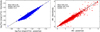 |
Fig. A.1 Comparison between the calculations of the power-law and the black-body models, for the fX (left panel) and IIN (right panel), for the sources included in the Good-fit sample of C2. |
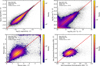 |
Fig. A.2 Comparison of fX (top-left panel), NH (top-right panel), photon index (bottom-left panel) and IIN (bottom-right panel) calculations between the C3 catalogue and C1, using the Good-fit subsets of the two catalogues. Each panel displays the mean, median difference, and scatter of the difference. |
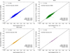 |
Fig. A.3 Comparison of fX calculations between the C4 catalogue and C1, categorised by source type in the C4 catalogue, for sources included in the Good-fit samples. Each panel displays the mean, median difference, and scatter. |
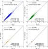 |
Fig. A.4 Comparison of IIN calculations between the C4 catalogue and C1, categorised by source type in the C4 catalogue, for sources included in the Good-fit samples. Each panel displays the mean, median difference, and scatter. |
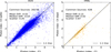 |
Fig. A.5 Comparison of Γ calculations between the C4 catalogue and C1, categorised by source type in the C4 catalogue, for sources included in the Good-fit samples. Each panel displays the mean, median difference, and scatter. |
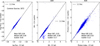 |
Fig. A.6 Comparison of fX (left panel), IIN (middle panel), and Γ (right panel) measurements for sources within the C4 catalogue, where the zpltb model is utilised for spectral fitting (i.e., AGNs), with corresponding measurements from C2, employing a power-law model for spectral fitting. Each panel displays the mean, median difference, and scatter. Sources included in the Good-fit samples are presented. |
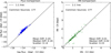 |
Fig. A.7 Comparison of fX and IIN calculations for sources within the C4 catalogue, where their X-ray spectra are fitted with a bbpl model (i.e., XRBs), and sources in the C2 catalogue fitted with a black-body model for their spectral analysis. Each panel displays the mean, median difference, and scatter. Sources included in the Good-fit samples are presented. |
Appendix B Catalogue column description
The four catalogues described in this paper correspond to four distinct FITS binary tables. Here we provide an overview of the information contained in the catalogues. Each row in the catalogues corresponds to a unique identifier given by either DETID (C1, C3), or SRCID (C2, C3), or a mixture of both (C4). For each unique identifier, we report on the background-model dependent camera net counts, camera usage, model parameter point estimate values, and supplementary information (such as degrees of freedom, p-value, and flag). Here we provide an overview of the naming convention used while the catalogues themselves and additional documentation are available on-line in CDS (see “Data availability”) and Zenodo:
The naming convention used for the camera counts and usage is as follows:
pn_cts – pn total counts in the source extraction area,
pn_bkgcts – pn counts in the background extraction area,
pn_netcts – pn net counts in the source extraction area,
pn_exp – pn exposure time in seconds,
mos_cts – MOS total counts in the source extraction area,
mos_bkgcts – MOS counts in the background extraction area,
mos_netcts – MOS net counts in the source extraction area,
mos_exp – MOS exposure time in seconds,
det_there – which cameras provide a spectrum 0: pn; 1: MOS; 2: pn and MOS,
det_use – which cameras are used for the fitting 0: pn; 1: MOS; 2: pn and MOS.
Each model is composed of one or more parameters. We use the following naming convention for the parameters:
lgflux – base-10 logarithm of the 0.2−12 keV flux in erg cm−2 s−1,
logNH – base-10 logarithm of the neutral hydrogen column density in cm−2,
PhoIndex – power-law photon index,
IIN – inter-instrument normalisation defined as MOS/pn,
kT – black-body/APEC/bremsstrahlung plasma temperature in keV,
logNorm – base-10 logarithm of the power-law normalisation in photons keV−1 cm−2 s−1 (C3 only).
For each model parameter, we report the median and the mode from the posterior distribution. For example, the median flux of the C1 power-law model is given by lgflux_med. We use the following naming convention for reporting the median and the mode of each model parameter:
med – median of the posterior distribution,
med_min – 5 per cent percentile of the posterior distribution,
med_max – 95 per cent percentile of the posterior distribution,
mod – mode of the posterior distribution,
mod_min – lower limit of the narrowest 90 per cent interval of the posterior distribution,
mod_max – upper limit of the narrowest 90 per cent interval of the posterior distribution.
Finally, the following additional columns are provided in order to estimate the quality of the model fit:
dof – degrees of freedom of the model fit,
pvalue – KS p-value of the source+background fit,
pval_bg_pn – χ2 p-value of the background fit for pn,
pval_bg_mos −χ2 p-value of the background fit for MOS,
flag – quality flag (described below).
The flag values 1 (no valid background counts), 2 (no valid net counts), 3 (unacceptable background fit) for C1, C2 and C3 are assigned to each spectrum as they appear in its processing, and each of them exclude the spectrum from further processing. The values assigned to each detection/source in the catalogues correspond to the highest value reached (i.e., the spectrum that reached the furthest processing stage) by the contributing pn and MOS spectra (or the value of the only spectrum that contributes).
For the catalogues C2 and C4, the model-dependent columns are suffixed by the name of the model e.g. lgflux_med_pl refers to the median of the flux of the power-law model, and pvalue_pl refers to the corresponding p-value. The model names used are:
pl – power-law model (C2 only),
bb – black-body model (C2 only),
zpltb – redshifted power-law model (C4 only),
apec_single – APEC model (C4 only),
bbpl – black-body + power-law model (C4 only),
bremss – bremsstrahlung model (C4 only). For C4, we provide the following additional columns:
D6 – entry flag 1: detection is from C1; 2: source is from C2,
classification – source classification according to Tranin et al. (2022). 0: AGN; 1: star; 2: XRB; 3: CV,
zbest – best available AGN redshift, defined as the spectroscopic redshift if available, else photometric redshift.
All Tables
Number of detections (C1, C3) or sources (C2, C4) included in each one of the four compiled catalogues.
Median values of (the mode of) each parameter for each source in the catalogues C1-4.
All Figures
|
Fig. 1 Distributions of the p-values (top-left panel), flux (top-right panel), NH (middle-left panel), photon index (middle-right panel), IIN (bottomleft panel) and black-body temperature (bottom-right panel) of the sources included in the Good-fit samples of C1, C2, and C3, as indicated in the legends. |
| In the text | |
|
Fig. 2 Distributions of the p-values (top-left panel), flux (top-right panel), NH (middle-left panel), IIN (middle-right panel), black-body temperature (bottom-left panel) and photon index (bottom-right panel) of the sources included in the Good-fit sample of C4. Blue lines present the results for AGNs (zpltb model), green lines display the measurements for stars (APEC model), orange lines show the calculations for XRBs (bbpl model) and red lines illustrate the results for CVs (bremss model). |
| In the text | |
|
Fig. 3 Distribution of 2−10 keV rest-frame intrinsic luminosity LX and redshift z of the reliable AGN sample. In the top panel, the grey and red dots correspond to unabsAGN and absAGN, respectively. Note that due to the discreteness of the zmode 0 from tpz (see the text for the details), the red-shift value plotted here is offset by a random number between −0.05 and 0.05. Bottom panels show the histograms of the redshift (left) and luminosity (right) of the Good-fit and reliable absAGN and unabsAGN samples. |
| In the text | |
|
Fig. 4 Fraction of absorbed AGNs as a function of redshift (top) and luminosity (bottom) both for the Good-fit AGN sample (grey dots) and for the reliable AGN sample (red triangles). |
| In the text | |
|
Fig. 5 Distribution of g−i (top), r−W2 (middle) and W1−W2 (bottom) colours of our reliable AGN samples, with absAGN in red and unabsAGN in grey. In the bottom panel we also show the simple W1−W2 colour criterion to select AGNs from Stern et al. (2005). |
| In the text | |
|
Fig. 6 WISE W1−W2 colour vs. W1 for reliable absAGN (red dots), unabsAGN (grey dots), XRBs (pink triangles), CVs (blue triangles), lowT stars (cyan squares), and highT stars (gold squares). The AGN locus (above the black line) of Assef et al. (2013) is also shown. |
| In the text | |
|
Fig. 7 Colour g−i vs. redshift for our reliable AGN sample: absAGN in red and unabsAGN in grey. |
| In the text | |
|
Fig. A.1 Comparison between the calculations of the power-law and the black-body models, for the fX (left panel) and IIN (right panel), for the sources included in the Good-fit sample of C2. |
| In the text | |
|
Fig. A.2 Comparison of fX (top-left panel), NH (top-right panel), photon index (bottom-left panel) and IIN (bottom-right panel) calculations between the C3 catalogue and C1, using the Good-fit subsets of the two catalogues. Each panel displays the mean, median difference, and scatter of the difference. |
| In the text | |
|
Fig. A.3 Comparison of fX calculations between the C4 catalogue and C1, categorised by source type in the C4 catalogue, for sources included in the Good-fit samples. Each panel displays the mean, median difference, and scatter. |
| In the text | |
|
Fig. A.4 Comparison of IIN calculations between the C4 catalogue and C1, categorised by source type in the C4 catalogue, for sources included in the Good-fit samples. Each panel displays the mean, median difference, and scatter. |
| In the text | |
|
Fig. A.5 Comparison of Γ calculations between the C4 catalogue and C1, categorised by source type in the C4 catalogue, for sources included in the Good-fit samples. Each panel displays the mean, median difference, and scatter. |
| In the text | |
|
Fig. A.6 Comparison of fX (left panel), IIN (middle panel), and Γ (right panel) measurements for sources within the C4 catalogue, where the zpltb model is utilised for spectral fitting (i.e., AGNs), with corresponding measurements from C2, employing a power-law model for spectral fitting. Each panel displays the mean, median difference, and scatter. Sources included in the Good-fit samples are presented. |
| In the text | |
|
Fig. A.7 Comparison of fX and IIN calculations for sources within the C4 catalogue, where their X-ray spectra are fitted with a bbpl model (i.e., XRBs), and sources in the C2 catalogue fitted with a black-body model for their spectral analysis. Each panel displays the mean, median difference, and scatter. Sources included in the Good-fit samples are presented. |
| In the text | |
Current usage metrics show cumulative count of Article Views (full-text article views including HTML views, PDF and ePub downloads, according to the available data) and Abstracts Views on Vision4Press platform.
Data correspond to usage on the plateform after 2015. The current usage metrics is available 48-96 hours after online publication and is updated daily on week days.
Initial download of the metrics may take a while.