| Issue |
A&A
Volume 704, December 2025
|
|
|---|---|---|
| Article Number | A308 | |
| Number of page(s) | 14 | |
| Section | Celestial mechanics and astrometry | |
| DOI | https://doi.org/10.1051/0004-6361/202555416 | |
| Published online | 06 January 2026 | |
Systemic recoil velocity distribution of field millisecond pulsar systems: Implications for neutron star retention in star clusters
1
Korea Astronomy and Space Science Institute,
776 Daedeokdae-ro, Yuseong-gu,
Daejeon,
Republic of Korea
2
Mizusawa VLBI Observatory, National Astronomical Observatory of Japan,
2-12 Hoshigaoka-cho, Mizusawa, Oshu,
Iwate 023-0861,
Japan
★ Corresponding author: This email address is being protected from spambots. You need JavaScript enabled to view it.
★★ EACOA Fellow.
Received:
7
May
2025
Accepted:
12
November
2025
Abstract
Aims. The systemic recoil velocity (vsys) distribution of millisecond pulsars (MSPs) is essential for understanding the MSP formation channel(s) and for estimating the retention fractions of MSPs in star clusters, which can potentially be determined using the precise astrometry of MSPs. However, the determination is complicated by the long-term dynamic evolution of MSPs and the scarcity of radial velocity measurements. The goal of this work is to overcome the complexity and derive the MSP vsys distribution from high-precision astrometric measurements.
Methods. We compiled 64 field MSP systems (including 52 binary MSPs and 12 solitary MSPs) that have been well determined astrometrically. We calculated their transverse peculiar (or space) velocities, v⊥, and Galactic heights, z. Assuming that the Galactic-longitude components, v1, of v⊥ are statistically stable over time (i.e. the ‘stable- v1’ assumption), we approached the distribution of the v1 components of vsys using the observed v1 sample. Under the ‘isotropic- vsys’ assumption that vsys directions are uniformly distributed, we derived the MSP vsys distribution from the distribution of the v1 component of vsys. Based on the derived vsys distribution, we tested the stable- v1 assumption with dynamical population synthesis (DPS). In addition, by matching the observed z and the Galactic-latitude components, vb, of v⊥ to the DPS counterparts, we estimated the initial and the current Galaxy-wide scale heights of field MSP systems.
Results. We find that solitary field MSPs have similar v1 magnitudes to those of binary ones. Additionally, the observed v1 can be well described by a linear combination of three normal distributions. Accordingly, the MSP vsys distribution can be approximated by a linear combination of three Maxwellian components. Our DPS analysis verified the stable- v1 assumption in the parameter space of this work and estimated the initial and the current Galaxy-wide scale heights of field MSP systems to be about 0.32 kpc and 0.68 kpc, respectively.
Conclusions. According to the MSP vsys distribution, ≈14% of all the MSPs born in a globular cluster with the nominal 50 km s−1 central escape velocity can be retained. Therefore, the vsys distribution of field MSP systems may account for the high number of MSPs discovered in globular clusters, which implies that MSPs in star clusters might follow the same formation channel(s) as field MSP systems.
Key words: astrometry / parallaxes / proper motions / stars: kinematics and dynamics / stars: neutron / pulsars: general
© The Authors 2026
 Open Access article, published by EDP Sciences, under the terms of the Creative Commons Attribution License (https://creativecommons.org/licenses/by/4.0), which permits unrestricted use, distribution, and reproduction in any medium, provided the original work is properly cited.
This article is published in open access under the Subscribe to Open model. This email address is being protected from spambots. You need JavaScript enabled to view it. to support open access publication.
1 Introduction
Compact stars are normally the dense remnants of stars that have exhausted their nuclear fuel, resulting in objects such as white dwarfs (WDs), neutron stars (NSs), and black holes (BHs). Distinct formation mechanism(s) have been proposed for different types of compact stars. For example, stellar BHs are believed to form mainly through either a direct collapse (of massive stars) or delayed collapse (e.g. Mirabel 2017). In the latter scenario, following a supernova explosion, a progenitor star’s core collapses into a proto-NS first, then succumbs to further collapse into a BH due to fallback accretion (e.g. Zhang et al. 2008). As another major form of compact stars, NSs can be born with core-collapse supernovae (CCSNe), while having alternative formation channels such as accretion-induced collapse (AIC; e.g. Tauris et al. 2013) and WD-WD mergers (e.g. Levan et al. 2006). Moreover, NSs encompass various subgroups such as magnetars and millisecond pulsar (MSP) systems, with each NS subgroup having its primary and alternative formation theories (e.g. Ding 2022).
As distinct formation channels of compact stars can lead to different natal kicks imparted to the compact star, kinematic investigations of compact stars hold the key to discriminating among different formation channels. This investigation can be realised with precise astrometry using space-based telescopes operating in the optical/infrared or through very long baseline interferometry (VLBI) observations made at radio, which has been pursued in the study of stellar BHs (e.g. Mirabel et al. 2002; Willems et al. 2005; Atri et al. 2019) and various NS subgroups (e.g. Tendulkar et al. 2013; Gonzalez et al. 2011; Ding et al. 2023, 2024b,c; Disberg et al. 2024b).
In practice, the birth velocity and position of a compact star or a compact star system (i.e. a gravitationally bound system of ≲3 stars hosting a compact star) can be derived with the knowledge of 1) the observed three-dimensional (3D) position; 2) the observed 3D velocity; and 3) the age of the system, by integrating the motion backward over time assuming a model of Galactic potential. However, the age of a compact star system is not usually well constrained and tends to require additional assumptions about the birth site (e.g. thin Galactic disk) of the compact star system (e.g. Fragos et al. 2009; Atri et al. 2019). Furthermore, most compact star systems, especially pulsar systems, do not have the information of line-of-sight radial velocities, vr. As a result, the investigation of the systemic recoil velocities, vsys, (the recoil velocities of lone compact stars or stellar systems hosting compact stars) of pulsar systems has mainly been limited to kinematically young (≲10 Myr old) systems (e.g. Cordes & Chernoff 1998; Kramer et al. 2003; Lorimer et al. 2006; Verbunt et al. 2017; Igoshev 2020; Ding et al. 2024c) to minimise the dynamic evolution (of the compact star systems) via the Galactic potential. We note that vr measurements are distinct from the so-called Galactic radial velocity, vR, defined as the radial component of motion in cylindrical Galactocentric coordinates. Unlike vr, vR can be precisely inferred from the transverse velocity of a compact star when the line of sight (to the compact star) is nearly perpendicular to the star’s radial vector in cylindrical Galactocentric coordinates.
On the other hand, for any specific subgroup of kinematically old (≳40 Myr) compact star systems that do not have vr information, the observed transverse peculiar velocities, v⊥, (also referred to as transverse space velocity; i.e. the velocity component tangential to the line of sight, with respect to the standard of rest of the neighborhood) is expected to deviate from the vsys component tangential to the sightline (e.g. Disberg et al. 2024a). Despite the deviation, it has been proposed by Faucher-Giguere & Kaspi (2006) that the Galactic-longitude component, v1, of v⊥ is statistically stable over time, which serves as a critical assumption that can link v1 to the vsys distribution. For this assumption to be validated in the parameter space of interest, dynamical population synthesis (DPS) is required, which simulates the motion of stellar objects through the Galactic potential assuming initial states (i.e. the positions and velocities; e.g. Cordes & Chernoff 1997).
Promising supreme timing stability, MSPs have been extensively studied and they are often used to test gravitational theories (e.g. Freire et al. 2012; Zhu et al. 2019; Freire & Wex 2024) and detect gravitational-wave background at the nanohertz (nano-Hz) regime (e.g. Agazie et al. 2023; Antoniadis et al. 2023a; Reardon et al. 2023; Xu et al. 2023; Miles et al. 2025). With spin periods of only ≲60 ms, MSPs are widely believed to have been spun up during the accretion from their respective donor stars. However, as explained in Section 1.3.1 of Ding (2022), the unexpectedly large number of MSPs retained in globular clusters (e.g. Pfahl et al. 2002) and possibly also at the Galactic centre (e.g. Abazajian & Kaplinghat 2012) suggest very small vsys of MSPs (e.g. Boodram & Heinke 2022), which reinforces exotic MSP formation channels such as the AIC channel (e.g. Gautam et al. 2022). Accordingly, it is likely that the MSP vsys distribution is multi-modal and/or multi-component (see Section 3 or Appendix C.1 for explanation), which has not been indicated by previous studies of MSP kinematics likely due to the relatively large astrometric uncertainties (Hobbs et al. 2005; Gonzalez et al. 2011).
Up till now, a well defined MSP vsys distribution remains largely absent, mainly due to the aforementioned technical challenges (i.e. long-term dynamic evolution and the lack of vr information) and relatively large astrometric uncertainties. This absence hinders the studies of MSP formation channels, and results in weak constraints on the NS retention fractions in star clusters. Recent years have seen a major increase in the number of well astrometrically determined MSPs (e.g. Ding et al. 2023; Shamohammadi et al. 2024), which is meant to offer a refined characterisation of the MSP vsys distribution. In this work, we have determined the MSP vsys distribution with the observed v1 calculated for 64 well astrometrically determined MSPs, then we discuss its implications for the NS retention fractions in star clusters. Throughout this paper, the uncertainties are stated at a 68% confidence level.
2 Observed transverse peculiar velocities and Galactic heights of MSPs
The establishment of the observed v⊥ distribution requires precise determination of both proper motions and distances for the MSPs, especially as MSP v⊥ are much lower than those of normal pulsars (Hobbs et al. 2005; Gonzalez et al. 2011; Matthews et al. 2016; Shamohammadi et al. 2024). Applying low-precision astrometric results to MSP kinematics studies would not only shift the average v⊥ to the higher end, but also reduce the ability to resolve the potential multiple modes in the v⊥ distribution. Compared to other methods, the determination of trigonometric parallaxes through VLBI astrometry (e.g. Ding et al. 2023), pulsar timing (e.g. Perera et al. 2019; Shamohammadi et al. 2024), or Gaia astrometry (e.g. Jennings et al. 2018; Moran et al. 2023), offers the most precise and reliable distances for MSPs. Recent releases of the astrometric results by Ding et al. (2023) and Shamohammadi et al. (2024) have significantly enriched the sample of well astrometrically determined MSPs, offering a rare opportunity to make statistically significant investigation of the MSP kinematics based purely on astrometrically well-determined MSPs.
We searched for viable MSPs across the PSRCAT catalogue1 (Manchester et al. 2005). Due to relatively frequent dynamic interactions inside globular clusters, the v⊥ values of globular cluster MSPs are not likely to be reflective of their vsys results. With globular cluster MSPs excluded from the study, we reached 64 field MSP systems having significant (>3 σ) proper motion and parallax determinations (see Table B.1). When only focusing on field MSPs with >5 σ and >7 σ parallaxes, we obtained two high-precision samples of 42 and 30 MSPs, respectively (see Appendix B). The details of the sample selection are described in Appendix A.
Following the methods detailed in Section 6 of Ding et al. (2023), we derived the distances d and the v⊥ of the 64 MSPs from their parallaxes and proper motions. The v⊥ values have been corrected for the Solar motion and converted to the local standard of rest of each pulsar. In deriving d from the parallaxes, the Lutz-Kelker bias (Lutz & Kelker 1973) has been systematically corrected. This correction is particularly important for MSPs with relatively low parallax significances (≲6 σ), as directly inverting parallaxes tends to underestimate their d (and likely v⊥ as well). From the d values, we calculated the Galactic heights z ≡ d sin b for the 64 MSPs, where b refers to Galactic latitudes. The derived d, v⊥, and z results are summarised in Table B.1, where the columns related to v⊥ include the v⊥ magnitudes, v⊥; the Galactic-longitude component, v1; and the Galactic-latitude component, vb, of v⊥. On top of v1 and vb, z serves as an additional indicator of MSP kinematics, as the average level of |z| expected to grow with higher vsys. Therefore, this work includes the studies of three samples of measurements: the vl, the vb, and the z samples.
Based on the calculations of the Pearson coefficients, no linear correlation was found between any two of the three samples. Accordingly, the three samples were treated independently. We conducted Wilcoxon signed-rank test on each of the three samples of 64 measurements, confirming that there was no indication of asymmetry about 0 in any sample. Accordingly, in the following analysis, we assumed that the samples of the observed v1, vb, and z are symmetric about 0.
Firstly, to visualise the three samples of measurements and, secondly, to investigate the underlying probability density function (PDF) for each sample, we assumed each measurement follows a split normal distribution, simulated 10 000 values per measurement, and concatenated the simulations into a chain of 640 000 values for each of v1, vb, and z. Despite the simulated sample of 640 000 following essentially a multi-modal distribution, the visualisation is expected to characterise where the measurements overlap. The resultant histograms are displayed in Figure 1. According to Table B.1 and Figure 1, most of the 64 MSPs are within the scale height of the Galactic thick disk (i.e. ∼ 1 kpc).
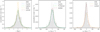 |
Fig. 1 Histograms of Galactic heights, z; the Galactic-longitude component, v1; and the Galactic-latitude component, vb, of transverse peculiar velocities, respectively shown in the left, middle, and right panels. Each histogram is concatenated from 10000 simulations drawn from the assumed split normal distributions for the 64 measurements (of z, vl, or vb; see Table B.1). The dashed grey curves show the normalised count smoothed with kernel density estimation (using scipy.stats.Gaussian_kde). The best-fit Cauchy, Laplace and three-component normal distributions are plotted as dashed blue and green curves. The dynamical population synthesis results (labelled as ‘evolved’) that best match the observed z, v1 and vb, based on the determined initial MSP scale height of ζ0=0.32 kpc, are overlaid. The corresponding initial distributions are also provided, except for v1, as the initial v1 distribution adopted in the dynamical population synthesis is identical to the best-fit three-component normal distribution (a linear combination of three normal distributions). |
2.1 Binary versus solitary
While most field MSPs are believed to be formed in binary systems where the NSs are spun up during the accretion from their main sequence companions (e.g. Alpar et al. 1982; Bhattacharya & van den Heuvel 1991) there are ≳20% of field MSPs found to have no companions. It is proposed that at least some of these solitary (or single) MSPs have ablated their companions after being spun up through accretion (e.g. Fruchter et al. 1988; Kluźniak et al. 1988). This scenario is supported by the discoveries of planets around the MSP PSR J1300+1240 (or PSR B1257+12) (Wolszczan & Frail 1992; Konacki & Wolszczan 2003) and planetary-mass companions around the MSPs PSRs J1719-1438 and J2322-2650 (Bailes et al. 2011; Spiewak et al. 2018). Additionally, the persistent achromatic component in the timing residuals of PSR J1939+2134 (or PSR B 1937+21) has been attributed to the presence of an asteroid belt surrounding the MSP (Shannon et al. 2013). Of the four aforementioned MSPs supporting the “companion ablation” scenario, PSRs J1300+1240 and J1939+2134 are included in this work, and they are classified as solitary MSPs (see Table B.1).
In addition to the companion ablation scenario, alternative theories have been proposed for the formation of solitary field MSPs, including (but not limited to) the AIC channel (Tauris et al. 2013; Freire & Tauris 2013) and the strange star scenario (Jiang et al. 2020). Particularly, the AIC channel is suggested to result in relatively small peculiar velocities (e.g. Gautam et al. 2022). Therefore, the precise astrometry of solitary MSPs can be used to potentially distinguish between the companion ablation and the AIC channels. Previous astrometric investigations by Hobbs et al. (2005); Gonzalez et al. (2011); Matthews et al. (2016); Shamohammadi et al. (2024) suggest no indication that solitary field MSPs and binary ones follow different v⊥ distributions. Here, we revisit the investigation in better detail, incorporating refined astrometric data and improved analytical techniques.
Among the 64 selected MSPs, 12 are solitary MSPs and 52 MSPs are in binary systems (see Table B.1). Following the aforementioned way of visualisation, we display the normalised histograms of vl, vb, and z for the 52 binary MSPs and 12 the solitary MSPs in Figure 2. The global magnitudes of v1, vb, and z of the solitary and the binary MSPs are summarised in Table 1. We found that the median and dispersion of |v1| of solitary MSPs agree with the counterparts of binary MSPs well. Assuming, firstly, that the v1 distribution is stable over time (see Section 4 for justification) and, secondly, that MSP systemic recoil velocities are equally possible in all directions, the agreement in |v1| suggests that solitary field MSPs could follow a systemic recoil velocity distribution similar to that of binary field MSPs. Accordingly, most solitary field MSPs are expected to follow the primary formation channel of binary MSPs (in which they are spun up through accretion from their companions), except that solitary field MSPs eventually evaporate their companions through irradiation. Though the AIC channel has been suggested to produce the bulk of the slow-moving MSPs that are presumably retained in the Galactic centre and contribute to the gamma-ray excess observed in the direction of the Galactic centre (Boodram & Heinke 2022; Gautam et al. 2022), the observed v1 suggest that the AIC channel should contribute little to the production of solitary field MSPs. In the following discussions, we assume that solitary and binary field MSPs share the same systemic recoil velocity distribution. We have been able to derive the systemic recoil velocity distribution with the full sample of 64 MSPs.
On the other hand, both the |z| and |vb| values of solitary MSPs appear to be overall smaller than the counterparts of the binary MSPs. In other words, binary MSPs are found to be more spread out from the Galactic plane (than solitary MSPs), with their |z| nearly following a uniform distribution between 0−1 kpc (see Figure 2). This spread may reflect the observational bias that searching for binary MSPs in the scattered low-Galactic-latitude sky regions is disproportionately harder (compared to solitary MSPs), which could be gradually resolved with increasingly advanced binary pulsar search techniques (e.g. Balakrishnan et al. 2022; Sengar et al. 2025). As the sample of solitary field MSPs remains small, we use the full sample of 64 MSPs to estimate the initial and the evolved scale heights of field MSPs in Section 4, which should be considered the weighted average values of the two sub-samples (of solitary and binary MSPs).
Global magnitudes of the Galactic heights and the transverse peculiar velocities of the binary and the solitary millisecond pulsars.
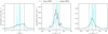 |
Fig. 2 Normalised histograms of the observed Galactic heights, z, Galactic-longitude component, vl, and Galactic-latitude component, vb, of transverse peculiar velocities (displayed as curves in the left, middle, and right panels, respectively) for 52 binary MSPs and 12 solitary MSPs (see Table B.1). The histograms have been smoothed with kernel density estimation using scipy.stats.Gaussian_kde. Each histogram is concatenated from 10 000 simulations drawn from the assumed split normal distributions for the measurements (of z, v1 or vb; see Table B.1). |
2.2 Modal analysis based on different parallax significance
Following the method detailed in Section 7.2.3 of Ding et al. (2024b), we ran Hartigan’s dip tests (Hartigan & Hartigan 1985) on the three samples (of 64 measurements) and found no indication of multi-modality in any of the samples. As the v1 distribution is believed to be stable over time (Faucher-Giguere & Kaspi 2006), we mainly discuss the dip tests on the v1 sample. When assuming that the v1 sample follows a distribution symmetric about 0 (as is supported by the aforementioned Wilcoxon signed-rank tests), the |v1| sample would, in principle, enhance the indicators of potential multi-modality. Should the v1 sample truly follow the multi-modal distribution used in the visualisation, about 180 and 240 additional v1 measurements would be needed to rule out uni-modality of the |v1| sample at 90% and 95% confidence, respectively, according to our simulations.
Additionally, we ran the same analysis on high-precision MSP samples obtained with higher thresholds of parallax significance ϖ/σϖ (see Appendix B). The results for v1 and |v1| are summarised in Table 2. According to Table 2, raising ϖ/σϖ thresholds reduces the MSP sample sizes and lowers the level of unimodality of |v1| or v1 measurements. The latter trend is likely caused by small sample effects. However, it is not unlikely that more high-precision astrometric measurements made with VLBI or pulsar timing could resolve the v1 distribution and reveal multimodality of MSP |v1| with certainty in the future. In the following discussion, we only focus on the full MSP sample (of 64) and assume that the v1 distribution is unimodal (given no indication of multi-modality).
p values (of unimodality) of Hartigan’s dip tests on MSP samples (with the sample size denoted as Nsample) obtained with various parallax significances, ϖ/σϖ.
3 The systemic recoil velocity distribution
We followed Faucher-Giguere & Kaspi (2006) to approach the vsys distribution with the observed v1 sample (see Table 2), assuming that v1 stays statistically stable over the long (≲10 Gyr) journeys of MSPs. The validation of this ‘stable-v1’ assumption is detailed in Section 4. We determined the vsys distribution in mainly three steps.
In the first step, we identified PDF candidates based on two simplifying assumptions. Given no indication that the observed v1 sample is multi-modal or asymmetric at about zero (see Section 2), we assumed that the underlying PDF of the observed v1 sample is both uni-modal and symmetric at about zero. Basic PDFs that meet these two requirements include (but are not limited to) normal distributions, Laplace distributions, and Cauchy distributions. Additionally, linear combinations of these basic distributions also serve as useful candidates. In particular, a linear combination of normal distributions with different scales (hereafter referred to as a multi-component normal distribution) would conveniently correspond to a multi-component Maxwell distribution for vsys (assuming that vsys is equally possible in all directions for kinematically old pulsar systems).
In the second step, we fit the parameter(s) of each candidate PDF using scipy.optimize.curve_fit (Virtanen et al. 2020) for the PDF to approximate the curve (see Figure 1) smoothed from the normalised histogram of the measurementbased simulated v1 sample of 640 000 (see Section 2), where the smoothing was conducted with kernel density estimation using scipy.stats.Gaussian_kde (Virtanen et al. 2020). After discarding candidates with poor fitting results, we identified two groups of prime PDF candidates (that match the normalised v1 histogram well), with one group comprised of linear combinations of Cauchy distributions and the other group made up of linear combinations of the normal distributions. The prime candidate PDFs are described in detail in Appendix C.1.
In the final step, we selected the PDF for the observed v1 sample by the method detailed in Appendix C.2. We conclude that the observed v1 can be well described by a Cauchy distribution with scale of 51.2 km s−1 (i.e. Equation (C.7)). Despite a three-component normal distribution being more consistent with the Cauchy distribution (see Figure 1), the more complex distribution has four more free parameters and, therefore, it is less favorable. On the other hand, the three-component normal distribution (described by Equation (C.2) and displayed in Table C.1) not only serves as a good approximation to the underlying PDF of the observed v1 sample, but it also provides a rare analytical solution for the vsys magnitude vsys. Specifically, when assuming the vsys distribution is isotropic for kinematically old pulsar systems, vsys is expected to follow a three-component Maxwell distribution (i.e. a weighted sum of three Maxwell distributions) that share the same parameters with the best-fit three-component normal distribution (see Table C.1). Namely, under the ‘isotropic- vsys’ assumption, vsys should approximately follow the PDF expression,
![Mathematical equation: $\begin{aligned}p=\sqrt{\frac{2}{\pi}} & \left\{0.463 \cdot \frac{v_{\mathrm{sys}}^{2}}{43.1^{3}} \cdot \exp \left[-\frac{1}{2}\left(\frac{v_{\mathrm{sys}}}{43.1}\right)^{2}\right]\right. \\& +0.477 \cdot \frac{v_{\mathrm{sys}}^{2}}{107.6^{3}} \cdot \exp \left[-\frac{1}{2}\left(\frac{v_{\mathrm{sys}}}{107.6}\right)^{2}\right] \\& \left.+0.060 \cdot \frac{v_{\mathrm{sys}}^{2}}{406.1^{3}} \cdot \exp \left[-\frac{1}{2}\left(\frac{v_{\mathrm{sys}}}{406.1}\right)^{2}\right]\right\},\end{aligned}$](/articles/aa/full_html/2025/12/aa55416-25/aa55416-25-eq7.png) (1)
(1)
where the unit of p and vsys is s km−1 and km s−1, respectively. In contrast, no analytical solution of the vsys PDF can be solved from the best-fit Cauchy distribution of v1. Therefore, we adopted Equation (1) as the vsys PDF in the following analysis, which is illustrated along with its cumulative distribution function (CDF) in Figure 3.
MSP velocities have been previously studied by Hobbs et al. (2005); Gonzalez et al. (2011); Matthews et al. (2016); Shamohammadi et al. (2024), where their MSP distances were mostly estimated using observed dispersion measures (DMs) and a model (Cordes & Lazio 2002; Yao et al. 2017) of the Galactic free electron distribution, as precise parallaxes were unavailable in most cases. Among these four works, Hobbs et al. (2005); Gonzalez et al. (2011) reported the mean 3D peculiar velocity of MSPs to be 111 ± 17 km s−1 and 108 ± 15 km s−1, respectively. Both values well agree with the median vsys (of field MSPs) estimated in this work (i.e. 105 km s−1; see Figure 3). Since no vsys distribution was derived in previous studies, a more detailed comparison with our vsys distribution is not currently feasible.
Regarding the use of Equation (1), we want to clarify two points. Firstly, despite the fact it is a three-component Maxwell distribution, Equation (1) is still a uni-modal distribution by definition (see Figure 3). Secondly, though approximating the vsys PDF by Equation (1), we do not suggest that field MSP systems have multiple formation channels. To further the investigation of formation channels of field MSP systems, population synthesis studies based on various MSP formation channels are needed to generate the theoretical vsys PDF templates that can be compared with our observation-based counterpart.
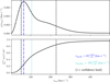 |
Fig. 3 Top: three-component Maxwell distribution described by Equation (1), which shares the parameters of the best-fit three-component normal distribution (see Table C.1) of the observed v1 sample. Bottom: cumulative distribution function (CDF) calculated from the threecomponent Maxwell distribution shown in the upper panel. The vertical dash-dotted line marks the mode of the three-component Maxwell distribution, while the dashed lines and the dotted line correspond to the 16th, the 84th, and the 50th percentile of the CDF, respectively. |
4 Dynamical population synthesis
When deriving the vsys PDF, we assumed v1 to be statistically stable over time (see Section 3). We tested this ‘stable- v1’ assumption using DPS that simulates the dynamics of field MSP systems in the Galaxy. Specifically, we like to examine if the current (or evolved) v1 distribution stays roughly the same as the initial v1 distribution. We used Equation (1) as the MSP vsys PDF in the DPS analysis. The MWPotential 2014 model, calculated and compiled into the galpy package by Bovy (2015), was adopted as the Galactic potential used in the DPS. Apart from the vsys PDF and the Galactic potential, two other ingredients are essential the DPS analysis: the MSP age distribution and the initial spatial distribution of field MSP systems in the Galaxy. The former ingredient is described in Appendix D.1, while the latter is introduced below.
4.1 The initial Galactic spatial distribution
The initial Galactic distribution of field MSP systems consists of two parts: the birth radial distribution (i.e. the spatial distribution projected to the Galactic plane) and the birth Galactic height distribution (hereafter referred to as the zi distribution). For the former, we adopted the pulsar radial distribution established with relatively young pulsars by Xie et al. (2024), assuming that field MSPs (excluding those originating from globular clusters) are born in pulsar-forming regions similar to those of younger pulsars (such as the spiral arms and the central Galactic region; Xie et al. 2024).
On the other hand, the zi distribution of field MSP systems is largely unknown. As we found that the observed z sample (see Table B.1) can be well described by a Laplace distribution with the scale height  (see Figure 1 and Appendix D.3.1), we assumed that zi of Galaxy-wide field MSP systems also follow a Laplace distribution with the scale height of ζ0. In DPS, we realised that both the evolved vb and the evolved z change with ζ0 (see Appendix D.3.2). Therefore, by matching the evolved vb and the evolved z to the observed counterparts, we can determine ζ0. The DPS procedure that determines the evolved states (including the evolved positions and the evolved velocities) is described in Section 4.2, while the details of the ζ0 determination are provided in Appendix D.3.2. We found that the DPS with ζ0=0.32 kpc renders evolved vb and evolved z samples that match the observed counterparts well (see Figure D.3). Accordingly, we adopted ζ0=0.32 kpc for the Galaxy wide zi distribution of field MSP systems.
4.2 The procedure of dynamical population synthesis
In DPS, we first simulated 10000 initial positions based on the initial spatial distribution described in Section 4.1. At each position, we assumed the stellar progenitor of the MSP followed circular motion (about the axis of rotation of the Galaxy) specified by the rotation curve of the MWPotential2014 Galactic potential model. The vsys results were simulated based on the vsys PDF (i.e. Equation (1)) and the ‘isotropic-vsys’ assumption (see Section 3). By adding the simulated vsys to the position-based circular velocities, we obtained the simulated MSP velocities with respect to the Galactic centre. Based on the simulated initial positions and velocities, we calculated the simulated initial v1, vb, and zi in the same way as the calculation of the observed counterparts. The histograms of the initial vb and zi samples were smoothed with kernel density estimation (using scipy.stats.Gaussian_kde) and overlaid on Figure 1. Since the three-component normal distribution we adopted as the initial v1 distribution is already displayed in Figure 1, we have not overlaid the smoothed histogram of the initial v1 sample.
Subsequently, we performed orbit integrations with galpy to obtain the evolved positions and velocities after the span of each age in the sample of 13005 MSP ages described in Appendix D.1. In this way, we were able to compile 10 000 × 13 005=130 million evolved states (i.e. positions and velocities for different MSP ages) of simulated MSPs, from which ∼ 4% evolved states outside the edge of the Galaxy (i.e. beyond 292 kpc from the Galactic centre, Deason et al. 2020) were discarded. To take into account the selection effect that leads to astrometrically well determined pulsars being predominantly located within ≲8 kpc, we removed evolved states that are beyond the 8 kpc distance. Additionally, given that the observed MSPs compiled in this work are ≲2.5 kpc from the Galactic plane (see Figure 1), we discarded the evolved states with |ze|>2.5 kpc, where ze refers to the evolved Galactic heights. The remaining evolved states are ∼ 37 million in number, which amount to ∼ 30% of the Galaxy-wide evolved states.
4.3 Results of dynamical population synthesis
From the remaining evolved states, we calculated the evolved v1, vb, and ze in the same way as the calculation of the observed counterparts (see Section 2 and references therein). We overlaid the results of the evolved vl, vb, and ze to Figure 1 in the same way as the initial counterparts. As is shown in Figure 1, the initial v1 distribution (labelled as ‘Tri-Normal’) is indeed consistent with the evolved v1 distribution, which validates the ‘stable- v1’ assumption (see Section 3) within the initial phase space of this study. Despite the validation, we reiterated the necessity of assessing the consistency between the initial and the evolved v1 on a case-by-case basis, especially in the regime where vsys and/or ζ0 are relatively large. In contrast, the distributions of evolved vb and ze are considerably different from the initial counterparts, which meets our expectation that the initial MSP zi would spread out over time, while the initial vb becoming weakened due to the pull of the Galactic potential.
Moreover, from the Galaxy-wide ze sample (of ∼ 125 million), we found that the best-fit scale height, ζ, for field MSP systems in the whole Galaxy is 0.68 kpc, which is 31% larger than the observed scale height,  , estimated from relatively nearby MSPs. Interestingly, unlike the observed z sample that is best described by a Laplace distribution (see Appendix D.3.1), the Galaxy-wide ze sample is best characterised by the Cauchy distribution with 0.48 kpc scale (see Figure D.4).
In our analysis, ζ0 and ζ1 were estimated based on the observed z and vb, without accounting for selection effects related to Galactic latitude (also see Appendix D.3.2). As noted in Section 2.1, the observed scale height of binary field MSPs is larger than solitary field MSPs. Therefore, the ζ0 and ζ1 estimated here should reflect the weighted average of the two sub-samples (of binary and solitary field MSPs). In the future, increasing MSP detections across the sky, driven by progressively advanced pulsar search techniques, will enable further refinement of ζ0 and ζ1.
5 The indicative millisecond pulsar retention fractions in star clusters
At the time of writing, about 345 pulsars (predominantly MSPs) have been found to be retained in 45 globular clusters (see the ‘Pulsars in Globular Clusters’ catalogue2). The high NS retention fraction of over 10-20% in globular clusters has been difficult to reconcile with the relatively large NS peculiar velocities (Cordes & Chernoff 1997; Toscano et al. 1999; Hobbs et al. 2005; Gonzalez et al. 2011) that are believed to easily exceed the generally small globular cluster central escape velocities (∼ 50 km s−1); this NS retention problem in globular clusters challenges the conventional NS formation theory (Pfahl et al. 2002). As the vast majority of pulsars detected in globular clusters are MSPs, the crux of the globular cluster NS retention problem is investigating why globular clusters host more MSPs than expected. However, the absence of the MSP vsys distribution has led to significant uncertainties in the investigation. Furthermore, while the mean 3D space velocities estimated for MSPs by Hobbs et al. (2005); Gonzalez et al. (2011) are consistent with our median vsys (see Section 3), the relatively large astrometric uncertainties in previous works would disproportionately inflate v⊥ at the lower end of their v⊥ distributions, which is expected to have lowered the predicted indicative rates of MSP retention in globular clusters.
Provided the null hypothesis that MSPs in star clusters follow the same formation channels (and accordingly the same vsys distribution) as field MSP systems, the vsys CDF (see Equation (C.8)) derived for field MSP systems can also be seen as the indicative MSP retention fraction as a function of the star cluster central escape velocity, vesc. At the nominal globular cluster vesc=50 km s−1, we would expect ≈14% of MSPs to be retained in the globular cluster, which is no longer inconsistent with the expected retention fraction range of roughly 10% to 20% for binary systems (Drukier 1996). The indicative MSP retention fraction would further rise to ≳48% for a globular cluster with exceptionally high vesc of ≳100 km s−1 (e.g. Terzan 5). Therefore, our MSP vsys distribution might be able to account for the large number of MSPs detected in globular clusters, potentially alleviating concerns regarding NS retention in globular clusters. Accordingly, we see no evidence that the aforementioned null hypothesis (i.e. that MSPs in star clusters follow the same formation channels as field MSP systems) would have been violated. A more accurate determination of the MSP retention fraction requires careful N-body simulations based on the MSP vsys distribution, which is beyond the scope of this work.
6 Summary and prospects
This work derives the systemic recoil velocity (vsys) distribution of field millisecond pulsar (MSP) systems from the observed v1 (i.e. the Galactic-longitude component of the transverse peculiar velocity), considering that 1) v1 is statistically stable over time based on the ‘stable v1’ assumption and 2) the vsys directions are uniformly distributed based on the isotropic vsys assumption). We found that the vsys distribution can be approximated by a linear combination of three Maxwellian distributions. Using dynamical population synthesis (DPS), we validated the stable v1 scenario and evaluated the initial and current Galaxy-wide scale heights of field MSP systems by matching the observed Galactic heights and v1 (i.e. the Galactic-latitude component of the transverse peculiar velocity) to the DPS counterparts. The MSP vsys distribution reported in this work predicts relatively large MSP retention fractions that could account for the large number of MSPs retained in globular clusters.
In light of the interesting discovery that the MSP vsys distribution can be well approximated by a linear combination of three Maxwellian components, we highly encourage the production of template vsys distribution for each formation channel using population synthesis that carefully simulates the MSP formation. These template vsys distributions can be used to make comparisons with the observation-based vsys distribution, thereby deepening the understanding of MSP formation. Finally, the methods described in this paper can be used to determine the vsys distribution and the scale height for other kinds of kinematically old compact stars (e.g. black hole systems) using precise astrometry (especially when radial velocity information is missing).
Acknowledgements
HD appreciates the helpful comments from the anonymous reviewer, and acknowledges the EACOA Fellowship awarded by the East Asia Core Observatories Association.
References
- Abazajian, K. N., & Kaplinghat, M., 2012, Phys. Rev. D, 86, 083511 [Google Scholar]
- Agazie, G., Anumarlapudi, A., Archibald, A. M., et al. 2023, ApJ, 951, L8 [NASA ADS] [CrossRef] [Google Scholar]
- Akaike, H., 2011, International Encyclopedia of Statistical Science, 25 [Google Scholar]
- Alam, M. F., Arzoumanian, Z., Baker, P. T., et al. 2020, ApJS, 252, 4 [NASA ADS] [CrossRef] [Google Scholar]
- Alam, M. F., Arzoumanian, Z., Baker, P. T., et al. 2021, ApJS, 252, 5 [Google Scholar]
- Alpar, M. A., Cheng, A. F., Ruderman, M. A., & Shaham, J., 1982, Nature, 300, 728 [NASA ADS] [CrossRef] [Google Scholar]
- Antoniadis, J., Arumugam, P., Arumugam, S., et al. 2023a, A&A, 678, A50 [NASA ADS] [CrossRef] [EDP Sciences] [Google Scholar]
- Antoniadis, J., Babak, S., Nielsen, A.-S. B., et al. 2023b, A&A, 678, A48 [NASA ADS] [CrossRef] [EDP Sciences] [Google Scholar]
- Arzoumanian, Z., Brazier, A., Burke-Spolaor, S., et al. 2018, ApJS, 235, 37 [CrossRef] [Google Scholar]
- Atri, P., Miller-Jones, J., Bahramian, A., et al. 2019, MNRAS, 489, 3116 [NASA ADS] [CrossRef] [Google Scholar]
- Bailes, M., Bates, S. D., Bhalerao, V., et al. 2011, Science, 333, 1717 [NASA ADS] [CrossRef] [Google Scholar]
- Balakrishnan, V., Champion, D., Barr, E., et al. 2022, MNRAS, 511, 1265 [NASA ADS] [CrossRef] [Google Scholar]
- Bangale, P., Bhattacharyya, B., Camilo, F., et al. 2024, ApJ, 966, 161 [Google Scholar]
- Bhattacharya, D., & van den Heuvel, E. P. J., 1991, Phys. Rep., 203, 1 [Google Scholar]
- Boodram, O., & Heinke, C. O., 2022, MNRAS, 512, 4239 [Google Scholar]
- Bovy, J., 2015, ApJS, 216, 29 [NASA ADS] [CrossRef] [Google Scholar]
- Camilo, F., Reynolds, J., Ransom, S., et al. 2016, ApJ, 820, 6 [NASA ADS] [CrossRef] [Google Scholar]
- Chatterjee, S., Brisken, W. F., Vlemmings, W. H. T., et al. 2009, ApJ, 698, 250 [NASA ADS] [CrossRef] [Google Scholar]
- Cordes, J., & Chernoff, D. F., 1997, ApJ, 482, 971 [Google Scholar]
- Cordes, J., & Chernoff, D. F., 1998, ApJ, 505, 315 [NASA ADS] [CrossRef] [Google Scholar]
- Cordes, J. M., & Lazio, T. J. W., 2002, arXiv preprint [arXiv:astro-ph/0207156] [Google Scholar]
- Crowter, K., Stairs, I. H., McPhee, C. A., et al. 2020, MNRAS, 495, 3052 [Google Scholar]
- Curyło, M., Pennucci, T. T., Bailes, M., et al. 2023, ApJ, 944, 128 [NASA ADS] [CrossRef] [Google Scholar]
- Deason, A. J., Fattahi, A., Frenk, C. S., et al. 2020, MNRAS, 496, 3929 [NASA ADS] [CrossRef] [Google Scholar]
- Deller, A. T., Archibald, A. M., Brisken, W. F., et al. 2012, ApJ, 756, L25 [NASA ADS] [CrossRef] [Google Scholar]
- Deller, A. T., Weisberg, J. M., Nice, D. J., & Chatterjee, S., 2018, ApJ, 862, 139 [NASA ADS] [CrossRef] [Google Scholar]
- Deller, A. T., Goss, W. M., Brisken, W. F., et al. 2019, ApJ, 875, 100 [NASA ADS] [CrossRef] [Google Scholar]
- Ding, H., 2022, PhD thesis, Swinburne University of Technology [Google Scholar]
- Ding, H., Deller, A. T., Stappers, B. W., et al. 2023, MNRAS, 519, 4982 [NASA ADS] [CrossRef] [Google Scholar]
- Ding, H., Deller, A. T., Freire, P. C., & Petrov, L. 2024a, A&A, 691, A47 [NASA ADS] [CrossRef] [EDP Sciences] [Google Scholar]
- Ding, H., Deller, A. T., Swiggum, J. K., et al. 2024b, ApJ, 970, 90 [Google Scholar]
- Ding, H., Lower, M. E., Deller, A. T., et al. 2024c, ApJ, 971, L13 [Google Scholar]
- Disberg, P., Gaspari, N., & Levan, A. J. 2024a, A&A, 687, A272 [NASA ADS] [CrossRef] [EDP Sciences] [Google Scholar]
- Disberg, P., Gaspari, N., & Levan, A. J. 2024b, A&A, 689, A348 [NASA ADS] [CrossRef] [EDP Sciences] [Google Scholar]
- Drukier, G., 1996, MNRAS, 280, 498 [Google Scholar]
- Faucher-Giguere, C.-A., & Kaspi, V. M., 2006, ApJ, 643, 332 [Google Scholar]
- Fiore, W., Levin, L., McLaughlin, M. A., et al. 2023, ApJ, 956, 40 [NASA ADS] [CrossRef] [Google Scholar]
- Fragos, T., Willems, B., Kalogera, V., et al. 2009, ApJ, 697, 1057 [NASA ADS] [CrossRef] [Google Scholar]
- Freire, P. C., & Tauris, T. M., 2013, MNRAS, 438, L86 [Google Scholar]
- Freire, P. C. C., & Wex, N., 2024, Liv. Rev. Relativ., 27, 5 [NASA ADS] [CrossRef] [Google Scholar]
- Freire, P. C. C., Wex, N., Esposito-Farèse, G., et al. 2012, MNRAS, 423, 3328 [NASA ADS] [CrossRef] [Google Scholar]
- Fruchter, A., Stinebring, D., & Taylor, J., 1988, Nature, 333, 237 [Google Scholar]
- Gautam, A., Crocker, R. M., Ferrario, L., et al. 2022, Nat. Astron., 6, 703 [CrossRef] [Google Scholar]
- Geyer, M., Krishnan, V. V., Freire, P., et al. 2023, A&A, 674, A169 [NASA ADS] [CrossRef] [EDP Sciences] [Google Scholar]
- Ginsburg, A., Sipőcz, B. M., Brasseur, C., et al. 2019, AJ, 157, 98 [NASA ADS] [CrossRef] [Google Scholar]
- Gonzalez, M., Stairs, I., Ferdman, R., et al. 2011, ApJ, 743, 102 [NASA ADS] [CrossRef] [Google Scholar]
- Guillemot, L., Smith, D., Laffon, H., et al. 2016, A&A, 587, A109 [NASA ADS] [CrossRef] [EDP Sciences] [Google Scholar]
- Hartigan, J. A., & Hartigan, P. M., 1985, Ann. Statist., 13, 70 [CrossRef] [Google Scholar]
- Hobbs, G., Lorimer, D., Lyne, A., & Kramer, M., 2005, MNRAS, 360, 974 [Google Scholar]
- Igoshev, A. P., 2020, MNRAS, 494, 3663 [NASA ADS] [CrossRef] [Google Scholar]
- Jennings, R. J., Kaplan, D. L., Chatterjee, S., Cordes, J. M., & Deller, A. T., 2018, ApJ, 864, 26 [NASA ADS] [CrossRef] [Google Scholar]
- Jiang, L., Wang, N., Chen, W.-C., et al. 2020, A&A, 633, A45 [NASA ADS] [CrossRef] [EDP Sciences] [Google Scholar]
- Kaplan, D. L., Kupfer, T., Nice, D. J., et al. 2016, ApJ, 826, 86 [NASA ADS] [CrossRef] [Google Scholar]
- Kiziltan, B., & Thorsett, S. E., 2010, ApJ, 715, 335 [Google Scholar]
- Kluźniak, W., Ruderman, M., Shaham, J., & Tavani, M., 1988, Nature, 334, 225 [NASA ADS] [CrossRef] [Google Scholar]
- Konacki, M., & Wolszczan, A., 2003, ApJ, 591, L147 [NASA ADS] [CrossRef] [Google Scholar]
- Kramer, M., Bell, J. F., Manchester, R. N., et al. 2003, MNRAS, 342, 1299 [NASA ADS] [CrossRef] [Google Scholar]
- Kramer, M., Stairs, I., Manchester, R., et al. 2021, Phys. Rev. X, 11, 041050 [NASA ADS] [Google Scholar]
- Levan, A. J., Wynn, G. A., Chapman, R., et al. 2006, MNRAS, 368, L1 [NASA ADS] [CrossRef] [Google Scholar]
- Lorimer, D. R., Stairs, I. H., Freire, P. C., et al. 2006, ApJ, 640, 428 [NASA ADS] [CrossRef] [Google Scholar]
- Lutz, T. E., & Kelker, D. H., 1973, PASP, 85, 573 [Google Scholar]
- Manchester, R., 2017, J. Astrophys. Astron., 38, 42 [NASA ADS] [CrossRef] [Google Scholar]
- Manchester, R. N., Hobbs, G. B., Teoh, A., & Hobbs, M., 2005, AJ, 129, 1993 [Google Scholar]
- Matthews, A. M., Nice, D. J., Fonseca, E., et al. 2016, ApJ, 818, 92 [NASA ADS] [CrossRef] [Google Scholar]
- Miles, M. T., Shannon, R. M., Reardon, D. J., et al. 2025, MNRAS, 536, 1489 [Google Scholar]
- Mirabel, F., 2017, New Astron. Rev., 78, 1 [CrossRef] [Google Scholar]
- Mirabel, I. F., Mignani, R., Rodrigues, I., et al. 2002, A&A, 395, 595 [NASA ADS] [CrossRef] [EDP Sciences] [Google Scholar]
- Moran, A., Mingarelli, C. M., Bedell, M., Good, D., & Spergel, D. N., 2023, ApJ, 954, 89 [Google Scholar]
- Ng, C., Guillemot, L., Freire, P., et al. 2020, MNRAS, 493, 1261 [Google Scholar]
- Perera, B., DeCesar, M., Demorest, P., et al. 2019, MNRAS, 490, 4666 [NASA ADS] [CrossRef] [Google Scholar]
- Pfahl, E., Rappaport, S., & Podsiadlowski, P., 2002, ApJ, 573, 283 [NASA ADS] [CrossRef] [Google Scholar]
- Pitkin, M., 2018, arXiv preprint [arXiv:1806.07809] [Google Scholar]
- Reardon, D., Shannon, R., Cameron, A., et al. 2021, MNRAS, 507, 2137 [CrossRef] [Google Scholar]
- Reardon, D. J., Zic, A., Shannon, R. M., et al. 2023, ApJ, 951, L6 [NASA ADS] [CrossRef] [Google Scholar]
- Reardon, D. J., Bailes, M., Shannon, R. M., et al. 2024, ApJ, 971, L18 [Google Scholar]
- Sengar, R., Bailes, M., Balakrishnan, V., et al. 2025, MNRAS, 536, 3159 [Google Scholar]
- Shamohammadi, M., Bailes, M., Flynn, C., et al. 2024, MNRAS, 530, 287 [Google Scholar]
- Shannon, R., Cordes, J., Metcalfe, T., et al. 2013, ApJ, 766, 5 [NASA ADS] [CrossRef] [Google Scholar]
- Spiewak, R., Bailes, M., Barr, E., et al. 2018, MNRAS, 475, 469 [Google Scholar]
- Spiewak, R., Bailes, M., Miles, M., et al. 2022, PASA, 39, e027 [Google Scholar]
- Stovall, K., Freire, P., Antoniadis, J., et al. 2019, ApJ, 870, 74 [NASA ADS] [CrossRef] [Google Scholar]
- Swiggum, J. K., Kaplan, D. L., McLaughlin, M. A., et al. 2017, ApJ, 847, 25 [Google Scholar]
- Tauris, T. M., Sanyal, D., Yoon, S.-C., & Langer, N., 2013, A&A, 558, A39 [NASA ADS] [CrossRef] [EDP Sciences] [Google Scholar]
- Tendulkar, S. P., Cameron, P. B., & Kulkarni, S. R., 2013, ApJ, 772, 31 [Google Scholar]
- Toscano, M., Sandhu, J., Bailes, M., et al. 1999, MNRAS, 307, 925 [NASA ADS] [CrossRef] [Google Scholar]
- van der Wateren, E., Bassa, C. G., Clark, C. J., et al. 2022, A&A, 661, A57 [NASA ADS] [CrossRef] [EDP Sciences] [Google Scholar]
- Verbunt, F., Igoshev, A., & Cator, E., 2017, A&A, 608, A57 [NASA ADS] [CrossRef] [EDP Sciences] [Google Scholar]
- Virtanen, P., Gommers, R., Oliphant, T. E., et al. 2020, Nat. Methods, 17, 261 [Google Scholar]
- Willems, B., Henninger, M., Levin, T., et al. 2005, ApJ, 625, 324 [NASA ADS] [CrossRef] [Google Scholar]
- Wolszczan, A., & Frail, D. A., 1992, Nature, 355, 145 [CrossRef] [Google Scholar]
- Xie, J., Wang, J., Wang, N., Manchester, R., & Hobbs, G., 2024, ApJ, 963, L39 [Google Scholar]
- Xu, H., Chen, S., Guo, Y., et al. 2023, RAA, 23, 075024 [NASA ADS] [Google Scholar]
- Yan, Z., Shen, Z.-Q., Yuan, J.-P., et al. 2013, MNRAS, 433, 162 [CrossRef] [Google Scholar]
- Yao, J. M., Manchester, R. N., & Wang, N., 2017, ApJ, 835, 29 [NASA ADS] [CrossRef] [Google Scholar]
- Zhang, W., Woosley, S. E., & Heger, A., 2008, ApJ, 679, 639 [NASA ADS] [CrossRef] [Google Scholar]
- Zhu, W., Desvignes, G., Wex, N., et al. 2019, MNRAS, 482, 3249 [Google Scholar]
Appendix A Selection of the millisecond pulsar sample
We selected the MSP sample from the PSRCAT catalogue1 (Manchester et al. 2005) with the help of the psrqpy Python package (Pitkin 2018). The MSPs were searched using the following criteria:
- (i)
P0<60 ms, where P0 represents the spin periods of MSPs;
- (ii)
Ṗ0<2 × 10⁻¹⁷ s s−1, where Ṗ0 denotes the time derivative of P0;
- (iii)
MSPs should not belong to globular clusters (as explained in Section 2);
- (iv)
and both proper motion magnitude and parallax are of >3 σ significance, with the uncertainty in the proper motion magnitude calculated through the propagation of uncertainties in the right ascension (RA) and the declination components.
There is no clear P0 boundary between MSPs and other pulsars. Various P0 upper limits up to ∼ 100 ms have been adopted in different studies of MSPs (e.g. Manchester 2017; Spiewak et al. 2022; Ding et al. 2023). In this work, we adopted the indicative P0 upper limit of 60 ms. Additionally, we followed Spiewak et al. (2022), applying the filter Ṗ0<2 × 10⁻¹⁷ s s−1 to exclude recently born (≲10 kyr old) pulsars (such as the Crab pulsar with 34 ms spin period), except for PSR J1417–4402 that does not have a reported Ṗ0. Despite the Ṗ0 being unknown to us, PSR J1417–4402 is suggested to have entered the late recycling phase (Camilo et al. 2016); therefore, it is likely to be kinematically similar to many other MSPs. Despite meeting all the requisite conditions, it has been suggested that PSR J1024–0719, which is in an unusually long-period orbit with a main sequence star, was born in (and ejected from) a globular cluster (Kaplan et al. 2016). Therefore, we removed PSR J1024–0719 from the MSP sample.
As mentioned in Section 2, we looked for field MSP systems with >3 σ parallax determinations. However, the Gaia-based astrometric results registered in the PSRCAT catalogue come from Jennings et al. (2018) based on the Gaia Data Release (DR) 2 (instead of the latest Gaia DR3). Therefore, in practice, we conducted the sample search in three steps. In the first step, we searched for MSPs with a discounted parallax significance threshold of 3 × 0.8=2.4, where 0.8 is the expected ratio of parallax precision between the Gaia DR3 and the Gaia DR2. In the second step, we updated the astrometric results of Jennings et al. (2018) to Gaia DR3 utilising the astroquery package (Ginsburg et al. 2019). In the final step, we removed MSPs with insignificant (<3 σ) determinations of parallaxes or proper motions. Compared to parallaxes, proper motions are usually determined at higher significance. The proper motion filter (as part of the criterion iv) only removes one MSP (i.e. PSR J1811–2405), which has been determined to be too close to the ecliptic plane to acquire precise proper motion in the declination direction with pulsar timing (Ng et al. 2020). Through the three-step procedure, we reached a sample of 64 field MSP systems, compiled in Table B.1, along with their most precise proper motion and parallax determinations. After calculating the transverse peculiar velocities v⊥ of the 64 MSPs (see Section 2), we found no correlation between P0 and v⊥, thereby indicating a negligible selection effect of P0 on v⊥.
Appendix B High-precision samples
For the selection of the main sample, the thresholds for the significance of proper motions and parallaxes are set to be relatively low (i.e. 3 σ), since raising the thresholds would inevitably favour high-proper-motion and nearby pulsars. Higher proper motions would likely correspond to larger transverse peculiar velocities v⊥. On the other hand, given no indication of correlation between v⊥ and MSP distances, raising the threshold of parallax significance could be rewarding: further lowering astrometric uncertainties, which are dominated by the distance uncertainties, might hold the key to potentially resolving multiple velocity modes. In order to investigate the impact of fractional parallax precision on the velocity analysis, we also adopted higher thresholds of parallax significance for sample selection. For example, with the 5 σ and the 7 σ thresholds of parallax significances, two ‘high-precision’ samples of 45 and 30 MSPs, respectively, were obtained for comparison with the full sample (of 64 MSPs) (see Table 2).
In the same way as described in Section 2, we compiled vl, vb, and z chains for the high-precision MSP samples, which are displayed in Figure B.1 along with the counterparts of the full sample. Compared to the full sample of 64 MSPs, the high-precision MSP samples render consistent v1, vb, and z distributions, while showing increasingly prominent substructures in the v1, vb, and z distributions as sample size drops, likely due to small sample effects.
Appendix C Determining the probability density function for v1
Appendix C.1 Candidate probability density functions of v1
Following the first and the second steps described in Section 3, we identified two prime groups of candidate probability density functions (PDFs) of v1. The first group is a linear combination of Cauchy distributions where the probability density p takes the form of
 (C.1)
(C.1)
while the second group being a linear combination of normal distributions, following the relation
 (C.2)
(C.2)
In this paper, we refer to Equations C.1 and C.2 as Cauchy series and Gaussian series, respectively. In either equation, γi is the scale of the i-th Cauchy or normal distribution. When N=1, Equations C.1 and C.2 are simplified to a Cauchy distribution and a normal distribution, respectively. For both groups, we refer to a PDF with N=2, 3, 4 as a two-component distribution, a three-component distribution, and a four-component distribution, respectively. The best-fit parameters for Equations C.1 and C.2 are provided in Table C.1.
Appendix C.2 Selecting from the candidate probability density distributions
From each of the two prime PDF groups introduced in Appendix C.1, we selected one v1 PDF based on a criterion that is equivalent to the Akaike information criterion (Akaike 2011). Specifically, the goodness Λ of a PDF is quantified by
 (C.3)
(C.3)
where L refers to the likelihood that the measurements match the PDF, and k represents the number of free parameters in the PDF. A PDF with higher Λ is considered better. For Equations C.1 and C.2,
 (C.4)
(C.4)
the likelihood L can be calculated by
 (C.5)
(C.5)
where  is the value of Equation C.1 or C.2 at the observed
  .
.
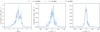 |
Fig. B.1 Normalised histograms of Galactic heights, z, the Galactic-longitude component, vl, and the Galactic-latitude component, vb, of transverse peculiar velocities, shown, respectively, in the left, middle, and right panels. The normalised histograms have been smoothed with kernel density estimation (using scipy.stats.Gaussian_kde). Each histogram is concatenated from 10000 simulations drawn from the assumed split normal distributions for the measurements (of z, v1 or vb; see Table B.1). The black, magenta, and yellow curves correspond to the full sample (of 64 field MSPs) and two high-precision samples (see Appendix B), respectively. |
Accordingly, the comparison of two PDFs is based on the Λ difference
 (C.6)
(C.6)
where K ≡ L1/L2 is the Bayes factor between the two PDFs. To evaluate the uncertainty in K due to the uncertainties in the 64 v1 measurements, we assumed the observed v1 follow split normal distributions, and simulated 10000 sets of 64 v1 values. From each set of 64 v1 values we derived a K based on Equation C.5. With the altogether 10000 derived K values, we estimated K and its uncertainty for two PDFs of comparison. The calculated ln K (as well as their uncertainties) of the candidate PDFs with respect to the best-fit Cauchy distribution are provided in Table C.1.
With larger N (and accordingly more free parameters), the PDF is expected to better approach the data, leading to larger K. Meanwhile, the incremental increase of ln K would quickly drop at larger N. For each of the two prime groups of candidate PDFs, we started fitting the PDF parameter(s) and estimating the corresponding K from N=1, then repeated the parameter fitting and K estimation at incrementally larger N until the incremental increase of ln K becomes negligible compared to 2 – the incremental increase of the number of free parameters. We found that Λ (defined by Equations C.3 through C.5) peaks at N=1 for the Cauchy series, and at N=3 for the Gaussian series (see Table C.1). In other words, the best-fit Cauchy distribution and the best-fit three-component normal distribution are selected for the two prime groups of candidate PDFs.
Between the two finalist PDFs, the Cauchy distribution is preferred over the three-component normal distribution according to the Λ standard (see Table C.1). Therefore, we conclude that the sample of 64 observed v1 is well described by the simple PDF
![Mathematical equation: $\frac{p}{1 \mathrm{~s} \mathrm{~km}^{-1}}=\frac{1}{51.2 \pi\left[1+\left(\frac{v_{\mathrm{l}}}{51.2 \mathrm{~km} \mathrm{~s}^{-1}}\right)^{2}\right]}.$](/articles/aa/full_html/2025/12/aa55416-25/aa55416-25-eq17.png) (C.7)
(C.7)
On the other hand, the three-component normal distribution is highly convenient for the calculation of the vsys distribution: when assuming vsys is statistically isotropic (in other words, equally possible in all directions) for kinematically old pulsar systems, the vsys magnitude vsys would follow a three-component Maxwell distribution with parameters identical to those of the three-component normal distribution (see Equation 1). Furthermore, the analytical solution,
![Mathematical equation: $\mathcal{F}\left(v_{\mathrm{sys}}\right)=\sum_{i=1}^{3} \alpha_{i}\left[\operatorname{erf}\left(\frac{v_{\mathrm{sys}}}{\sqrt{2} \gamma_{i}}\right)-\sqrt{\frac{2}{\pi}} \cdot \frac{v_{\mathrm{sys}}}{\gamma_{i}} \exp \left(-\frac{v_{\mathrm{sys}}{ }^{2}}{2 \gamma_{i}^{2}}\right)\right],$](/articles/aa/full_html/2025/12/aa55416-25/aa55416-25-eq18.png) (C.8)
(C.8)
can be derived for the cumulative distribution function (CDF) of the three-component Maxwell distribution, where erf is the error function, and the parameters αi and γi can be found in Table C.1. The three-component Maxwell distribution as well as its corresponding CDF is displayed in Figure 3. In comparison, provided the same ‘isotropic- vsys’ assumption, no closed-form solution of vsys can be obtained when each direction of vsys follows a Cauchy distribution. Therefore, we consider the three-component normal distribution a good and useful approximation to Equation C.7 and the v1 PDF.
Appendix D Supplementary materials on dynamical population synthesis
Appendix D.1 Millisecond pulsar age distribution
The age distribution of MSPs is poorly constrained. We approached the rough MSP age distribution by the following procedure. Firstly, we identified MSPs from the PSRCAT1 catalogue with the MSP criteria (i) and (ii) stated in Appendix A. After removing sources without constraint on characteristic age τc, we obtained 399 MSP τc values. To derive the age distribution, we corrected the τc sample by a sample of age correction factors (i.e. ratio between age and τc) estimated by Kiziltan & Thorsett (2010) for 42 MSPs having proper motion measurements (i.e. the reciprocals of  reported in Table 1 of Kiziltan & Thorsett 2010). Specifically, we multiplied each of the τc sample by each of the correction factor sample, which led to a sample of 399 × 42=16758 MSP ages. After discarding ages larger than the age of the Galaxy (i.e. 13.6 Gyr), we obtained a sample of 13 005 MSP ages (see Figure D.1 for the histogram of this sample). We considered this age sample as an indicative approximation to the MSP age distribution, and adopted the age sample in the DPS analysis (see Section 4.2).
Despite the yet poorly constrained MSP age distribution, we find that the DPS results are insensitive to the uncertainties in the age distribution (see Appendix D.2). While this insensitivity reinforces the robustness of the DPS results, it also prohibits the possibility of constraining age distribution of MSPs (and likely other kinematically old compact star systems) through astrometric studies.
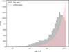 |
Fig. D.1 Gray: Histogram of the millisecond pulsar age distribution adopted in DPS (see Appendix D.1), with logarithmically spaced bins along the x-axis; Pink: Uniform distribution 𝒰(0.1, 13.6)(Gyr) with logarithmically spaced bins along the x-axis, which is only used to examine the DPS robustness with respect to uncertainties in the MSP age distribution (see Appendix D.2). |
Appendix D.2 The robustness with respect to uncertainties in the age distribution
To investigate the impact of the uncertainties in the MSP age distribution on the DPS results, we reran DPS with the same setup except for the MSP age distribution. For the rerun, we adopted the uniform distribution 𝒰(0.1, 13.6) (Gyr) as the MSP age distribution (i.e. the ages are evenly distributed between 0.1 Gyr and 13.6 Gyr), which is overlaid to Figure D.1 in order to show its deviation from the age distribution of reference. Despite the difference between the uniform distribution and the reference distribution, we find that the two distinct age distributions render almost identical DPS results (see Figure D.2). Therefore, we conclude that the DPS results are robust with respect to the uncertainties in the MSP age distribution.
Appendix D.3 Supplementary materials on the determination of the birth Galactic height distribution
Appendix D.3.1 The underlying probability density function of the observed Galactic heights
When searching for the candidates for the underlying PDF of the observed z sample, we assumed that the PDF is both unimodal and symmetric about zero. The same assumptions had been adopted in identifying the underlying PDF for the observed v1 (see Section 3). We found that the one-parameter Cauchy distribution and the one-parameter Laplace distribution are both plausible candidates for the underlying PDF of the observed z (see Figure 1). However, further analysis following the method detailed in Appendix C.2 prefers the best-fit Laplace distribution over the Cauchy counterpart with ln  , where K is the Bayes factor. The best-fit Laplace distribution for the observed z sample has the scale height
  of 0.52 kpc. We note that
  is derived from nearby field MSP system, which should be distinguished from the scale height ζ1 of Galaxy-wide field MSP systems.
Appendix D.3.2 The determination of the Galaxy-wide birth scale height, ζ0
As mentioned in Section 4.1, various ζ0 would lead to different levels of the evolved vb and ze. Due to the complex distributions of the observed z and vb (see Figure 1 or Figure D.3), we find it difficult to determine the ζ0 using statistical methods (e.g. Kolmogorov-Smirnov tests or the Wasserstein metric) that quantify the similarity between the observed samples and the DPS counterparts. On the other hand, the evolved scale height  is expected to increase with ζ0 (see Figure D.3), and match the observed counterpart
  (see Appendix D.3.1). Therefore, we reran the DPS with incrementally larger ζ0 until the best-fit
  reaches 0.52 kpc. In this way, we found ζ0 ≈0.32 kpc. The dependence of the evolved vb, ze and v1 on ζ0 is illustrated in Figure D.3. As is shown in Figure D.3, both the evolved vb and ze match the observed counterparts at ζ0= 0.32 kpc. Additionally, the average levels of both evolved |b| and |ze| rise with ζ0 as expected. In comparison, the evolved v1 stays robust with respect to changes in the birth vertical distribution of field MSP systems.
Finally, we note that the observed z sample might be biased by Galactic latitude-related selection effects. As a major example, pulsars located at low Galactic latitudes, b, are more susceptible to propagation effects caused by the ionised interstellar medium (IISM), which might reduce the detection rate of these low-|b| pulsars. This relative drop in the number of low-|b| pulsars would become increasingly significant as furtheraway pulsars are searched and observed with large telescopes. In Section 2.1, we found that the observed scale height of binary field MSPs is larger than solitary field MSPs, which may indicate the larger difficulty to detect binary MSPs (compared to solitary MSPs) in scattered low-|b| sky regions. On the other hand, most pulsar search programs have been focusing on low-|b| sky regions, which serves as another selection effect that would increase the relative number of low-|b| pulsars. We note that we did not take into account the impact of complex b-related selection effects on the observed z (and vb) in this work.
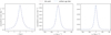 |
Fig. D.2 Difference between the smoothed histogram profiles of evolved ze, vl and vb based on two distinct MSP age distributions: the uniform distribution 𝒰(0.1, 13.6) (Gyr) in blue and the MSP age distribution described in Appendix D.1. |
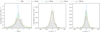 |
Fig. D.3 Smoothed histogram profiles of z, vl, and vb derived from dynamical population synthesis based on different Galaxy-wide birth scale height ζ0 of field MSP systems. Overlaid are the visualised histograms (and their smoothed profiles) of the observed z, vl, and vb (see Section 2). |
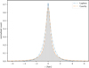 |
Fig. D.4 Histogram of Galaxy-wide evolved Galactic heights, ze, derived from dynamical population synthesis. Overlaid are the best-fit Laplace and Cauchy distributions of the ze sample, with the scale parameters of 0.68 kpc and 0.48 kpc, respectively. |
Distances, d, Galactic heights, z, transverse peculiar velocities, v⊥ ≡(vl, vb), and their magnitudes, v⊥, of the 64 selected millisecond pulsars calculated from their published proper motions (μα and μδ) and parallaxes, ϖ.
All Tables
Global magnitudes of the Galactic heights and the transverse peculiar velocities of the binary and the solitary millisecond pulsars.
p values (of unimodality) of Hartigan’s dip tests on MSP samples (with the sample size denoted as Nsample) obtained with various parallax significances, ϖ/σϖ.
Distances, d, Galactic heights, z, transverse peculiar velocities, v⊥ ≡(vl, vb), and their magnitudes, v⊥, of the 64 selected millisecond pulsars calculated from their published proper motions (μα and μδ) and parallaxes, ϖ.
All Figures
|
Fig. 1 Histograms of Galactic heights, z; the Galactic-longitude component, v1; and the Galactic-latitude component, vb, of transverse peculiar velocities, respectively shown in the left, middle, and right panels. Each histogram is concatenated from 10000 simulations drawn from the assumed split normal distributions for the 64 measurements (of z, vl, or vb; see Table B.1). The dashed grey curves show the normalised count smoothed with kernel density estimation (using scipy.stats.Gaussian_kde). The best-fit Cauchy, Laplace and three-component normal distributions are plotted as dashed blue and green curves. The dynamical population synthesis results (labelled as ‘evolved’) that best match the observed z, v1 and vb, based on the determined initial MSP scale height of ζ0=0.32 kpc, are overlaid. The corresponding initial distributions are also provided, except for v1, as the initial v1 distribution adopted in the dynamical population synthesis is identical to the best-fit three-component normal distribution (a linear combination of three normal distributions). |
| In the text | |
|
Fig. 2 Normalised histograms of the observed Galactic heights, z, Galactic-longitude component, vl, and Galactic-latitude component, vb, of transverse peculiar velocities (displayed as curves in the left, middle, and right panels, respectively) for 52 binary MSPs and 12 solitary MSPs (see Table B.1). The histograms have been smoothed with kernel density estimation using scipy.stats.Gaussian_kde. Each histogram is concatenated from 10 000 simulations drawn from the assumed split normal distributions for the measurements (of z, v1 or vb; see Table B.1). |
| In the text | |
|
Fig. 3 Top: three-component Maxwell distribution described by Equation (1), which shares the parameters of the best-fit three-component normal distribution (see Table C.1) of the observed v1 sample. Bottom: cumulative distribution function (CDF) calculated from the threecomponent Maxwell distribution shown in the upper panel. The vertical dash-dotted line marks the mode of the three-component Maxwell distribution, while the dashed lines and the dotted line correspond to the 16th, the 84th, and the 50th percentile of the CDF, respectively. |
| In the text | |
|
Fig. B.1 Normalised histograms of Galactic heights, z, the Galactic-longitude component, vl, and the Galactic-latitude component, vb, of transverse peculiar velocities, shown, respectively, in the left, middle, and right panels. The normalised histograms have been smoothed with kernel density estimation (using scipy.stats.Gaussian_kde). Each histogram is concatenated from 10000 simulations drawn from the assumed split normal distributions for the measurements (of z, v1 or vb; see Table B.1). The black, magenta, and yellow curves correspond to the full sample (of 64 field MSPs) and two high-precision samples (see Appendix B), respectively. |
| In the text | |
|
Fig. D.1 Gray: Histogram of the millisecond pulsar age distribution adopted in DPS (see Appendix D.1), with logarithmically spaced bins along the x-axis; Pink: Uniform distribution 𝒰(0.1, 13.6)(Gyr) with logarithmically spaced bins along the x-axis, which is only used to examine the DPS robustness with respect to uncertainties in the MSP age distribution (see Appendix D.2). |
| In the text | |
|
Fig. D.2 Difference between the smoothed histogram profiles of evolved ze, vl and vb based on two distinct MSP age distributions: the uniform distribution 𝒰(0.1, 13.6) (Gyr) in blue and the MSP age distribution described in Appendix D.1. |
| In the text | |
|
Fig. D.3 Smoothed histogram profiles of z, vl, and vb derived from dynamical population synthesis based on different Galaxy-wide birth scale height ζ0 of field MSP systems. Overlaid are the visualised histograms (and their smoothed profiles) of the observed z, vl, and vb (see Section 2). |
| In the text | |
|
Fig. D.4 Histogram of Galaxy-wide evolved Galactic heights, ze, derived from dynamical population synthesis. Overlaid are the best-fit Laplace and Cauchy distributions of the ze sample, with the scale parameters of 0.68 kpc and 0.48 kpc, respectively. |
| In the text | |
Current usage metrics show cumulative count of Article Views (full-text article views including HTML views, PDF and ePub downloads, according to the available data) and Abstracts Views on Vision4Press platform.
Data correspond to usage on the plateform after 2015. The current usage metrics is available 48-96 hours after online publication and is updated daily on week days.
Initial download of the metrics may take a while.